Potential and Problems of the Development of Speed Traffic on the Railways of Uzbekistan

Abstract

The chapter deals with the features of the organization of high-speed train traffic on existing Uzbek railways. The possibility of preserving and increasing the carrying capacity of high-speed railways with the combined movement, of freight and passenger trains, as well as the influence of speed traffic on the construction and technological parameters of individual parts and structural elements infrastructure of the railway, from the position of ensuring traffic safety at high-speed railways of Uzbekistan is analyzed in the article. The results of the research can be useful in studying, designing and operating a railway track of high-speed roads under similar conditions.

1 Basics of the Development of High-Speed Traffic in Uzbekistan

In the conditions of constant and rapid growth of population mobility, the possibility of their more active and unhindered movement, the problem of choosing the most reliable, convenient and economical means of transport arises.

Based on the criteria of safety, comfort all weather, speed or time on the way, regularity and cost of the trip, high-speed railway traffic is one of the most promising areas of passenger traffic in regions with a high population density.

In this regard, the priority direction of the development of railways in the world is the increase in the speed of passenger trains, the creation of a network of high-speed railways.

In Europe, the creation of a network of national high-speed railways that meets the requirements of the EU Directive EC 96/48 [1] is one of the promising areas for the development of passenger transport. By early 2017, high-speed rail lines have built and successfully operated in 21 countries, of the world, their total length is more than 21 thousand km [2,3,4]. Since 2011, Uzbekistan has been included in the list of countries with high-speed train traffic, where Talgo-250 trains began to run.

The development of integration processes in the world, the expansion of business, cultural, economic and tourist ties, is a constantly acting factor, which causes the growth of requirements for high-speed rapid pace, and, according to expert forecasts, by 2020 the length of the high-speed network will reach 25,000 km [4, 5]. The longest in the world inter-regional high-speed railway line Beijing-Shanghai length of 1320 km [6].

In the long term, China plans to provide a network of domestic high-speed rail lines to neighboring countries, namely, in the northwest of the country via Urumqi and Alashankou to the settlement of Druzhba in Kazakhstan, and also through Jinghe towards Alma-Ata, exit through Kyrgyzstan to Uzbekistan [4, 6, 7].

Thus, Uzbekistan, located in the central part of the Eurasian continent, will be at the center of the transcontinental railway communication from the Pacific to the Atlantic Ocean, which is a modern interpretation of the “Great Silk Road”.

The development of railways on the territory of the Republic of Uzbekistan dates back to 1874, when a special commission recognized the need for the construction of the Orenburg-Tashkent railway line. However, later in 1880 the decision was changed. Tashkent was connecting to the eastern coast of the Caspian Sea. Five years later, the builders reached Ashgabat, and in 1886 Chorzhou. In 1888, a movement was open up to Samarkand along the wooden bridge across the Amu Darya. In 1899 the road reached Tashkent. Simultaneously, a section was built from the Ursatievskaya station (now Khavast) to the Fergana valley.

At the end of the nineteenth century, the question arose again about the construction of a road from Tashkent to Orenburg, the construction of which began in the autumn of 1900 simultaneously from Tashkent and Orenburg. In 1906 the Tashkent-Orenburg road entered service, opening a direct exit to Central Russia for Central Asia.

After the acquisition of the country’s independence, the priority and the main direction of the development of railways was the creation of a unified network of railway communications. In 1993, the Government of the Republic of Uzbekistan adopted the General Program for the Electrification of Railways, according to which the electrification of the main lines was provided for in the shortest possible time, and further the electrification of the whole rail network.

The first step in the implementation of this program was the construction in 1993–2003 line Uchkuduk–Nukus, and the second step was construction in 2008–2011 line Guzar-Boysun-Kumkurgan. Construction in 2015–2016 the Angren-Pap line has completed the creation of a unified railway network of Uzbekistan’s transport infrastructure, ensuring the development of the productive forces of the regions, the development of their rich natural resources.

At the beginning of the 21st century, there were major changes in the passenger traffic. In order to increase the comfort of passenger transportation and bring them to the level of world standards, since 2004, the electric train “Registon” has started to run between Tashkent and Samarkand, since 2005 on the Tashkent-Bukhara line the “Shark” high-speed train, and on the Tashkent-Karshi route the high-speed train “Nasaf” with an average speed of 120 km/h.

The introduction in August 2011 of the high-speed passenger train Afrasiyob (Talgo-250 electric train) on the Tashkent-Samarkand line, in August 2015 on the Tashkent-Karshi line and in August 2016 on the Samarkand-Navoi-Bukhara line showed, that there are technical opportunities and progressive methods of organization and management of high-speed, train traffic are developed, ensuring the safety and trouble-free operation of trains with maximum speeds of up to 250 km/h and more (Fig. 1).

Fig. 1

High-speed electric train Talgo-250

At present, the construction of the Bukhara-Miskin line with the transfer by 2020 to electric traction is completed, which will allow to organize in Uzbekistan a national network of high-speed railways with a length of more than 1000 km (Fig. 2).

Fig. 2

The scheme of high-speed railways in Uzbekistan

The increase in the speed of passenger trains on the railways of JSC “Uzbekistan Temir Yollari” is carried out on the existing line (after their reconstruction and modernization) with the adjoining on some sections to new lines.

One of the most difficult issues in the introduction of high-speed train traffic is, first of all, bringing permanent technical means and railway infrastructure in line with the requirements imposed on them.

The problem lies in the following:

• the need to combine the movement of freight and passenger trains;

• the railway line was designed for a much lower load-carrying capacity, lower speed and weight of trains;

• the presence of a real tendency to further increase the intensity of freight trains.

Therefore, the organization of high-speed traffic on the railways of Uzbekistan means their transfer to a qualitatively higher level of transport services. This laid the foundation for a new stage of reconstruction and modernization of Uzbekistan’s railway transport.

As a result of the reconstruction of railways, their reliability and quality of work has significantly increased, and the indicators of rolling stock use have been improved due to significant capital expenditures.

Modernization of railway lines for the implementation of high-speed train traffic requires significant investments in volume, and their payback is a long time. Currently, private investors are not ready for such an investment. Therefore, in the Republic of Uzbekistan the creation of the infrastructure of high-speed railways was largely undertake by the state, having formulated the following requirements for the projects of creating a national network of high-speed railways:

• (1) when developing long-term plans for the development of a network of high-speed railways to improve their profitability, focus on its integration in the West through other countries of Central Asia and Russia, into a pan-European network; in the east—through Kyrgyzstan to the network of high-speed railways in China; in the south through Afghanistan, Turkmenistan, Iran to the network of high-speed railways of Turkey and Eastern Europe;

• (2) take into account the experience of creating a network of national high-speed railways of the countries of the European Union, Japan, China;

• (3) develop their own strategy for the implementation of projects for the reconstruction and modernization of the infrastructure of existing railways and the construction of new lines to organize the movement of high-speed trains.

It can be assumed that there are solutions that allow you to get the expected result at a much lower cost.

2 Construction and Technological Parameters of the Railway for High-Speed Train Traffic

The current regulatory documents of Uzbekistan set the maximum speed on high-speed railways within the limits of 141–200 km/h, on high-speed 201–250 km/h.

World experience shows that the highest speed of 200–350 km/h can be achieved by organizing high-speed train traffic on specialized high-speed lines. However, the construction of specialized high-speed railways and the production of specialized rolling stock for them requires large capital investments.

In cases of non-obvious positive effect of the introduction of high-speed train traffic on specialized lines, it is possible to consider the organization of high-speed passenger traffic on existing lines with combined movement of freight and passenger trains with speeds of:

• up to 120 km/h—on traditional railway lines;

• up to 160 km/h—on the lines after the road overhaul;

• up to 200 km/h—on the reconstructed lines.

The infrastructure of the railway line, where high-speed trains are used, should ensure their safe movement at the set speeds; the technical parameters of all of its facilities, track facilities, communications and computer facilities, automatics and teleautomatics, electrification and power supply and civil structures must comply with the design standards for high-speed railways. The basic requirements and standards for designing high-speed railways in Uzbekistan are given in [8, 9].

The construction and technological parameters of each structural element of the existing railway infrastructure determine the maximum level of speed of high-speed trains that must correspond to their state. A thorough study of the existing condition and construction and technological parameters of the existing rail infrastructure will allow to establish the maximum permissible speed of high-speed trains; Identify objective causes and factors that limit the speed of train traffic.

Since in Uzbekistan the organization of high-speed train traffic is carried out using the existing infrastructure, we will consider in more detail the construction and technological parameters of the railroad for high-speed railways.

The increase in the speed of train traffic on existing railways in Uzbekistan is complicated by a number of circumstances, the most important of which are the following:

• all previously constructed railways in the territory of modern Uzbekistan were designed based on the maximum train speed of no more than 120 km/h;

• for all main highways (main routes), the mixed movement of passenger and freight trains, with different levels of maximum speed, is characteristic;

• the increase in the maximum train speed to 140–160 km/h is associated with a significant amount of work on the reconstruction and modernization of the infrastructure of existing lines.

The increase in the speed of passenger trains on existing lines is hampered by a number of factors, the main of which are availability:

• numerous small-radius curves;

• inconsistencies in the design of the upper structure of the track, the contact network and traction substations, communication and signaling devices, the requirements;

• Old-style switches that do not allow the trains to follow them in the forward direction with the highest possible speed;

• the short length of the rails laid in the way, adversely affecting the characteristics of interaction between the rolling stock and the track, and also reducing the level of comfort for passengers.

Since it is not possible to carry out a radical reconstruction of all infrastructure facilities of existing lines that are part of the program for increasing the speed of trains in a relatively short time and with minimal costs, a rolling stock with a tilted body of cars designed for high-speed traffic along the existing track infrastructure is used.

To achieve the intended (given) level of speed, a number of measures and works on the modernization (reconstruction) of permanent devices and railway structures should be performed. These structures and devices include: the upper structure of the track, the roadbed, the system of signaling and communication, power supply, man-made structures, passenger platforms and other structures.

The main technical solutions that can be applied in the modernization and reconstruction of the infrastructure of existing railways are presented in Table 1.

Table 1 The main technical solutions recommended for the modernization and reconstruction of the infrastructure of existing lines

The increase in the speed of passenger trains is a stable global trend in the development of rail transport. At the same time, the first stage is the organization of high-speed passenger trains on existing lines with speeds of 160–200 (250) km/h after reconstruction and modernization of the railway infrastructure.

Instrumental research of the existing state of the railway allows the causes of the speed limits to be determined on each individual section of the railway; outline activities (or adopt a project solution) to eliminate them; determine the scope of work on the reconstruction (modernization) of certain structural elements of the railway infrastructure that limit the speed of high-speed passenger trains.

The total amount of work to eliminate both local and linear speed limits can’t be reduced to a single meter. Therefore, the scope of work is expedient to determine by types of restrictions, type of devices and structures.

As a rule, the amount of work to eliminate linear restrictions is actually equal to the length of the section where high-speed traffic of passenger trains is introduced, which is confirmed by the experience of organizing high-speed train traffic on the Tashkent-Samarkand, Samarkand-Bukhara section.

The scope of work for the introduction of high-speed train traffic using the existing railway infrastructure on the same site varies significantly depending on the maximum speed level to which the speed should be increased.

For example, from the existing maximum speed of 120 km/h to 140, 160, 200 km/h. Used in practice devices for signaling, power supply, VSP structures and others are designed for different levels of maximum speed, compliance in the gradation of speed in them are absent. So, for example, SCS devices for speeds up to 140 km/h, individual elements of the power supply infrastructure up to 120 km/h, etc.

Thus, there is a functional relationship between the established maximum speed of high-speed passenger trains and the construction and technological parameters of railway infrastructure facilities. Those. The established (preset) maximum speed level of high-speed trains, determines the construction and technological parameters of railway infrastructure facilities that ensure the safe movement of trains at a specified speed. It can be said in another way that the installed construction and technological parameters of railway infrastructure facilities determine the maximum level of speed of safe movement of high-speed trains. Then the established maximum speed level of high-speed trains also determines the scope of work for the reconstruction and reconstruction of the infrastructure of existing railways.

As a rule, high-speed traffic introduced on existing railways without significant changes to the existing infrastructure. In this case, the construction and technological parameters of the route plan, which were set for small speeds, are the main obstacle to increasing the speed of passenger trains.

In some countries where existing high-speed lines have been adapted for high-speed train traffic, it has been ascertained that increasing there speed above 220–230 km/h requires costly technologies in operating and maintaining the track and entails many technical and organizational difficulties. Therefore, the construction of a dedicated high-speed railway is the only way to increase the speed of passenger trains over 200 km/h.

In the directive documents, high-speed rail transport is considered as a single technological complex (railway track, railway power supply, railway automation and telemechanic, railway telecommunications, and station buildings, structures and devices), including subsystems of the natural and technical infrastructure of high-speed rail transport and safe traffic specialized high-speed railway rolling stock with speeds of 6 than 200 km/h.

Thus, the adopted construction and technological parameters of all subsystems of the natural and technical infrastructure of high-speed transport should ensure the safe movement of high-speed rolling stock at speeds exceeding 200 km/h.

As an example, consider the construction and technological parameters of the section of the Tashkent-Angren-Pap-Andijan railway, which, according to experts, will eventually become an element of high-speed ground communication between Europe and Asia along the international transport corridor “Southeast Asia–Western Europe” interstate [10,11,12,13].

Presumably, the high-speed traffic of passenger trains from Tashkent to Andijan can be organized along two routes (Fig. 3); within the Tashkent region and the Kamchik pass along the single route Tashkent-Angren-Pap; in the Ferghana Valley, from the Pape station to the Andijan station, according to variants of Pap Namangan-Andijan or Pap-Kokand-Andijan, which can be conditionally designated as “northern” and “southern” options. The length of the “northern” variant is 43 km shorter than the “southern” option.

Fig. 3

The scheme of the railway Tashkent-Andijan

To assess the options for organizing high-speed traffic, the analysis of the parameters of the technical equipment of infrastructure devices and structures, longitudinal profile elements and the plan of the railway section was carried out. According to the construction and technological parameters of the technical equipment of the railway section from the Tashkent station to the station of Andijan can be divided into the following four components:

Tashkent-Angren (T-A); Angren-Pap (A-P); Pap-Namangan-Andijan (P-N-A) and or Pap-Kokand-Andijan (P-K-A).

As shown by the analysis, the construction and technological parameters of the sections (Table 2) of the northern and southern variants of the Fergana ring movement are identical and on the longitudinal profile the longitudinal slopes are ranked in ascending order and distributed within the slopes 0.1–6, 6.1–9, 9.1–12, 12.1–18, 18.1–21, 21.1–24, 24.1‰ and more. The total length of the elements corresponding to a certain range of longitudinal slopes and their percentage as a percentage of the total length of sections of the railway are determined. A graphical representation of the distribution of the slopes of the longitudinal profile in these ranges and the fraction of the total length of the elements in them along separate sections shown in Fig. 4.

Table 2 Technical specifications section of the railroad Tashkent-Andijan

Fig. 4

Distribution of slopes of longitudinal profile elements

Analysis of the longitudinal profile of railways shows that in the Angren-Pape section, the total length of the longitudinal profile elements designed with slopes steeper than 12‰ is 52.3%, incl. 29.7% slopes steeper than 24‰. On the sections of Tashkent-Angren, Pap-Namangan-Andijan, Pap-Kokand-Andijan, maximum longitudinal deviations do not exceed 12–15‰. Thus, only on the Angren-Pape section, the speed of passenger trains can be limit by the path profile. However, for modern locomotives and electric trains, like Uzbekistan (production of China) or Talgo-250, this factor is not limiting and subsequent calculations, this factor can be ignore.

In the same way, in increasing order, the parameters of the elements of the plan are ranked, i.e. the length of the straight sections of the path (including the straight inserts between adjacent curves) and the radii of the circular curves; their number and proportion of the total number of elements of the plan.

Graphical representation of the distribution of the number of straight inserts and straight sections of the path, as well as the radii of circular curves for individual sections is shown in Figs. 5 and 6.

Fig. 5

The ratio of the number of straight inserts and straight sections of the path

Fig. 6

Correlation of radii of circular curves

The number of sections with a length of straight inserts and straight sections of a path of less than 300 m in Angren-Pap is 62%. In the other three areas, this indicator is almost two or more times less.

Analyzing the data characterizing the parameters of the elements of the plan, we can state that the main deterrent cause of the increase in the speed of passenger trains on the existing Tashkent-Andijan railway is the parameters of the elements of the route plan, and, first of all, the radii of the circular curves, and on the Angren-Pap sections length of straight inserts between adjacent curves.

Insufficient length of straight inserts does not allow, place transitional curves of longer length, accelerate to a higher speed. At the same time, the smooth running of the train along the curves is also disturbed, as a consequence, the comfort for passengers is worsened.

On the sections of Tashkent-Angren, Pap-Namangan-Andijan, Pap-Kokand-Andijan, more than half of the straight sections of the road allow placing the transitional curves of the calculated length and raising the outer rail to the normative value.

Almost half (46%) of the curves in the Angren-Pape plot are projected with a radius of 300 m or less. At the Tukimachi-Angren section, 22% of the curves have a radius of 301–400 m. At the Tukimachi-Angren, Pap-Namangan-Andijan, Pap-Kokand-Andizhan sections, the curves with a radius of 501–800 m, respectively, are 28, 36, 25%.

Appropriate calculations were carried out to evaluate the possibility of increasing the speed of passenger trains on existing sections of the Tashkent-Angren, Angren-Pap, Pap-Namangan-Andijan, Pap-Kokand-Andijan railroads [14] based on the following conditions and assumptions:

• 1. Rolling stock

  • for passenger trains electric locomotives O’zbekiston (production of China) and 4-axle wagons;

  • for high-speed trains of the Talgo-250 electric train.

• 2. Maximum permissible speeds

  • at the initial state of 70 km/h;

  • after the modernization of 90, 120, 140, 160, 180, 200 km/h.

• 3. Maximum driving speeds

  • passenger trains up to 140 km/h;

  • high-speed passenger trains 141–200 km/h.

• 4. Weight of formulations

  • passenger trains of 1200 ton;

  • high-speed passenger trains of 400 ton.

• 5. The maximum speed of freight trains with a combined movement of 70–90 km/h.

• 6. The highest value of the unprecedented acceleration is according to the norm 0.7 m/s².

• 7. The maximum elevation of the outer rail is 150 mm.

• 8. The rate of increase of the unoccupied acceleration in the transition curves, not more than 0.5–0.7 m/s²;

• 9. The speed of the passage of the switches is the same as the maximum permissible speed established in this section;

• 10. The whole area of Tashkent-Andijan is electrified.

• 11. To increase the maximum speed of passenger trains, it is planned to upgrade the permanent devices and infrastructure of the railway. At the same time, at this stage of the calculation, investments to modernize the permanent facilities and infrastructure facilities of the railway sections were not taken into account.

• 12. Calculations were carried out for both individual sections and for two variants of the route of the high-speed train, suggesting that trains along the whole route follow without stopping.

A distinctive feature of the single-track section of the Tashkent-Andijan railway is the combined movement of trains of all categories. Therefore, the maximum speed limit for train trains along the curves is established taking into account the safety and smoothness of movement of all the categories of trains that are circulating in this sector, including the Talgo-250 high-speed electric train with the car body tilt. Calculation of the parameters of the curve, equally satisfying the conditions for the movement of trains with maximum speeds, was performed in the same sequence as in [15]. The results of the calculations are summarized in Table 3.

Table 3 Time and speed of the train along sections

Based on the analysis of the parameters of the plan elements, the longitudinal profile, the results of the traction calculations carried out, the following were established:

• 1. The reasons for speed limits at the level of 90, 120, 140, 160, 180 and 200 km/h;

• 2. Separate sections, where it is possible to set the maximum speed of passenger trains at the level of 120, 140, 160, 180 and 200 km/h;

• 3. Separate sections, curves or adjacent curves at which the maximum speeds of passenger trains with available track parameters should be limited to speeds of 90, 120 km/h.

Calculations show that improving the construction and technological parameters of the track, i.e. the removal of speed limits for passenger trains on all sections, with the exception of the Angren-Pap section, allows the average speed of trains to reach 110–150 km/h, reducing the time spent on the road by 3.9 h (i.e., reducing by 40%).

The most intensive reduction of train travel time and accordingly an increase in the average speed occurs within the maximum speed of 70–160 km/h (Fig. 7). In the subsequent speed range of 160–200 km/h, the increase in average speed and, correspondingly, the shorter travel time of the train, occur less intensively.

Fig. 7

Changes in train travel time

A similar analysis was carried out when studying the construction and technological parameters of the Karshi-Kitab (Shakhrisabz), Karshi-Toshguzar-Boysun-Kumkurgan.

3 Features Safety for the Movement of High-Speed Trains

To increase the speed of trains in the 50–60 years of the last century, great efforts have been made to conduct research to increase the power of the power plant (engines) of diesel locomotives, electric motors of electric locomotives and electric trains. All resources, both intellectual and material, were aimed at increasing the energy component of locomotives and electric trains. At the same time, the study of air currents arising around the train, to study their physics was considered a secondary task.

A further increase in the speed of trains led to a qualitative change in the physics of air flows around high-speed trains, the transformation of train energy into aerodynamic resistance, noise and vibrations (vibrations) and other phenomena adversely affecting the dynamics of a high-speed train. As the speed increased, their character changed greatly.

At relatively low speeds, many theoretical problems and technical problems in the development of high-speed trains concerning (relative to) passenger discomfort, aerodynamic drag, noise, vibrations, pulse strength, and others arising during the movement (single and towards each other in parallel way) of high-speed trains.

An essential problem of further increasing the speed of trains is the aerodynamic resistance of the train. To increase the speed of high-speed trains, the aerodynamic drag must be kept as low as possible, which is associated with air currents arising around the moving train (Fig. 8). Depending on the place of their occurrence and the impact on the environment (objects), they can be conditionally divided into five groups:

Fig. 8

Air flows around the high-speed train

• air flows near the nose (head car) of the train;

• air flows along the train;

• air flows behind the train;

• air flows under the train;

• air flows over the train.

In addition, complex flows arise when moving high-speed trains along parallel paths, towards each other, and also when driving in a tunnel. The origin and impact of each of these flows has its own patterns. In sum, they form a complex in nature and diverse in their impact air flow, which must be considered in a complex and integrated into a single task.

Scientists from Europe, USA, Japan, China, Korea, Russia and others are conducting experimental and theoretical studies on the study of aerodynamics of a high-speed train and related issues [16,17,18,19]. The purpose of the research is to obtain aerodynamic data on the dynamics of the movement of high-speed trains, assess their impact on other trains, as well as on people in proximity to the passing train. So successfully solve the issues of the shape of the nose of the train to reduce the resistance to movement of the train [20,21,22,23,24].

Among the diverse studies of aerodynamics of a high-speed train, the problem of the interaction of the aerodynamic field of a high-speed train on the environment, for example, on the sandy surface and infrastructure elements near the railway track, and people on the platform remain unresolved. First of all, it is required to theoretically investigate the velocity field around a moving high-speed train.

The problem is the peculiarities of the movement of trains, which do not allow us to use the laws of the physics of aircraft. These features are as follows:

• the length of a moving train is much greater than its width;

• the train moves along a predetermined trajectory (along the railway track);

• the train moves in close proximity (along) the railway infrastructure facilities: top track elements, booths, contact-line towers (overhead lines), overpasses, bridges, station buildings, etc.;

• the train can move in a confined space (tunnel);

• a moving train through the flow of air affects the surface of the earth, a train moving toward or along a parallel path, people on a platform.

Currently, the speed of high-speed trains is approaching 300–350 km/h. The maximum speed of high-speed trains, which are in constant operation, reached 380–400 km/h. The speed record in the “rail-wheel” system is 574.8 km/h.

Increasingly relevant for high-speed train traffic is the study of their aerodynamic impact on people, railway infrastructure objects that are located near the passing train, ensuring their safety by applying scientifically based design standards for railway infrastructure facilities.

The introduction of high-speed passenger train traffic on the Tashkent-Samarkand section and the further expansion of the high-speed train range requires the improvement of certain sections of the current design standards for high-speed and high-speed railways in Uzbekistan [8, 9, 25, 26]. This, first of all, concerns the establishment (normalization) of the minimum permissible distance of the location of individual objects of the infrastructure of railways and people (passengers, railway workers) from the axis of the high-speed railway.

To establish the location (determine the minimum permissible distance) of railway infrastructure objects and people (passengers, railway workers), the effect of aerodynamic pressure on them, theoretical studies of the propagation of the velocity field around a high-speed train were carried out.

Below we analyze the distribution of the aerodynamic field around a high-speed train as an axisymmetric body with a head and tail in the form of a cone or come to life, moving in a compressible medium (Fig. 9), at a fixed point M(x, y, z). Since the motion of the body occurs along the axis, the change in the position of the center of the moving train relative to point M is taken into account by the introduction of a moving coordinate system $z = z_{1} - v_{0} t$, as shown in Fig. 3 [27].

Fig. 9

Scheme of motion of an axisymmetric body in a half-space

The components of the velocities of the particles of the medium along the coordinate axes 0z and 0r are determined in terms of the velocity potential by the formulas $\varphi_{1} (r,z_{1} ,t)$

$$ v_{z} = \frac{{\partial \varphi_{1} }}{\partial z},\quad v_{r} = \frac{{\partial \varphi_{1} }}{\partial r} $$

(1)

The equation for the propagation of an acoustic wave in the air can be written in the form

$$ \frac{{\partial^{2} \varphi_{1} }}{{\partial t^{2} }} = a^{2} (\frac{{\partial^{2} \varphi_{1} }}{{\partial r^{2} }} + \frac{1}{r}\frac{{\partial \varphi_{1} }}{\partial r} + \frac{{\partial^{2} \varphi_{1} }}{{\partial z_{1}^{2} }}). $$

(2)

Equation (2) can be reduced to the following form

$$ \alpha^{2} \frac{{\partial^{2} \varphi_{1} }}{{\partial z^{2} }} - \frac{{\partial^{2} \varphi_{1} }}{{\partial r^{2} }} - \frac{1}{r}\frac{{\partial \varphi_{1} }}{\partial r} = 0, $$

(3)

where, $\alpha - \alpha = \sqrt {1 - M^{2} } ,\,M = v_{0} /a$—Mach number.

Equation (3) is integrated under the following boundary conditions:

• 1. The condition of the non-slipping of air particles on the surface of the body:

  $$ v_{r} = \frac{{\partial \varphi_{1} }}{\partial r} = v_{0} \,tg\,\gamma \quad {\text{at}}\;r = f_{1} (z), $$

  (4)

  where $tg\,\gamma$ the equation of the surface of the body; the slope of the tangent to surfaces of a moving body.

  The equation of the surface of a body can be determined by the formulas $tg\,\gamma = f_{1}^{{\prime }} (z),\,f_{1} (z) = f_{1} ( - z)$. The value of the angle of inclination can vary within $0 \le \gamma \le 90^{ \circ }$.

• 2. The condition that the component along the axis 0y The velocity of the particles of the medium at the boundary of the half-space is determined from (5)

  $$ \frac{{\partial \varphi_{1} }}{\partial y} = 0\quad {\text{at}}\;y = - h - f_{1} (z) $$

  (5)

• 3. The symmetry condition with respect to the axis 0z

  $$ \varphi_{1} = 0\quad {\text{at}}\;z = 0 $$

  (6)

To find the solution of the equation, the method of sources [28]. Considering the function $\varphi (r,z)$, satisfying the Eq. (2) and the boundary condition (4), the solution can be represented in the form (7)

$$ \varphi = - \frac{1}{4\pi }\int\limits_{ - L}^{L} {\frac{q(\xi )d\xi }{{\sqrt {(\xi - z)^{2} + \alpha^{2} r^{2} } }}} $$

(7)

where $q(z)$—the power of a source distributed over the surface of a moving body within $0 < r < f_{1} (z),\, - L < z < L$.

For a thin axisymmetric body from formula (7), proceeding from [28], it can be asserted that:

• at $r \to 0\quad \frac{\partial \varphi }{\partial r} \to \frac{q(z)}{2\pi r}$;

• at $0 < z < L\;q(z) = 2\pi v_{0} f_{1}^{{\prime }} (z)\,f_{1} (z)$;

• at $- L < z < 0\quad q(z) = - 2\pi v_{0} f_{1}^{{\prime }} ( - z)\,f_{1} ( - z)$.

Then the function $\varphi (r,z)$ becomes (8)

$$ \varphi = - \frac{{v_{0} }}{2}(\int\limits_{ - L}^{0} {\frac{{f_{1}^{{\prime }} ( - \xi )\,f_{1} ( - \xi )\,d\xi }}{{\sqrt {(\xi - z)^{2} + \alpha^{2} r^{2} } }}} + \int\limits_{0}^{L} {\frac{{f_{1}^{{\prime }} (\xi )\,f_{1} (\xi )\,d\xi }}{{\sqrt {(\xi - z)^{2} + \alpha^{2} r^{2} } }})} $$

(8)

Given that $f_{1} ( - \xi ) = f_{1} (\xi ),\,f_{1}^{{\prime }} ( - \xi ) = - f_{1}^{{\prime }} (\xi )$ the Eq. (8) can be represented in the following form

$$ \varphi = - \frac{{v_{0} }}{2}(\int\limits_{0}^{L} {\frac{{f_{1}^{{\prime }} (\xi )\,f_{1} (\xi )\,d\xi }}{{\sqrt {(\xi + z)^{2} + \alpha^{2} r^{2} } }} - } \int\limits_{0}^{L} {\frac{{f_{1}^{{\prime }} (\xi )\,f_{1} (\xi )\,d\xi }}{{\sqrt {(\xi - z)^{2} + \alpha^{2} r^{2} } }})} $$

(8’)

In this case, the function $\varphi_{1} (r,z)$ can be represented in the following form (9)

$$ \varphi_{1} = \varphi (z,r) + \varphi (z,r_{1} ) $$

(9)

where $r_{1} = \sqrt {x^{2} + [2f_{1} (z) + 2h + y]^{2} }$.

It can be shown that the function represented by (9) $\varphi_{1} (r,z)$ satisfies all the conditions of the problem under consideration. The components of the velocity vector of air particles in a Cartesian coordinate system at an arbitrary point in space are expressed by the following formulas (10)–(12)

$$ \nu_{x} = \frac{{\partial \varphi_{1} }}{\partial x} = \left( {\frac{\partial \varphi (z,r)}{\partial r}\frac{\partial r}{\partial x} + \frac{{\partial \varphi (z,r_{1} )}}{{\partial r_{1} }}\frac{{\partial r_{1} }}{\partial x}} \right), $$

(10)

$$ \nu_{y} = \frac{{\partial \varphi_{1} }}{\partial y} = \left( {\frac{\partial \varphi (z,r)}{\partial r}\frac{\partial r}{\partial y} + \frac{{\partial \varphi (z,r_{1} )}}{{\partial r_{1} }}\frac{{\partial r_{1} }}{\partial y}} \right), $$

(11)

$$ \nu_{z} = \frac{{\partial \varphi_{1} }}{\partial z} = \frac{\partial \varphi (z,r)}{\partial z} + \frac{{\partial \varphi (z,r_{1} )}}{\partial z}. $$

(12)

As an example, we consider a body of revolution, the initial and final parts of which are cones and come to life. The shape of a moving body in the meridian plane is shown in Fig. 10. In this case, the accepted body dimensions are equal to the following values:

Fig. 10

Arrangement in the meridian plane of an axisymmetric body with the shape of the head and tail parts in the form: a cone; b came to life

• distance L from the middle of the moving body Oz;

• distance from the middle of the moving body to the initial point of shape change (outlines) of the head parts of the moving body $L_{0}$;

• cross-section of an axisymmetric body R;

• the cross section of the moving body is considered as a circle with a radius R of 2 m, the area of which is equal to the cross-sectional area of the train with a width of 3.0 m and a height of 4.0 m is 12 m^2;

• the angle of the cone of the head and tail is equal to $\gamma = 0.1538$ radius.

Functions $f_{1} (z)$ and $f_{1}^{{\prime }} (z)$ for the conical shape of the head and tail parts of the body, when $\gamma_{0} \approx tg\,\gamma_{0} = R/(L - L_{0} )$ are represented as follows:

• at $- L \le z \le - L_{0} ,\quad f_{1} = \gamma_{0} (L + z),\quad f_{1}^{{\prime }} = \gamma_{0}$;

• at $- L_{0} \le z \le L_{0} ,\quad f_{1} = R,\quad f_{1}^{{\prime }} = 0$;

• at $L_{0} \le z \le L,\quad f_{1} = \gamma_{0} (L - z),\quad f_{1}^{{\prime }} = - \gamma_{0}$.

For an axisymmetric body with a shape of the head and tail parts in the form, the functions $f_{1} (z)$ and $f_{1}^{{\prime }} (z)$ have the following form:

at $- L \le z \le - L_{0}$,:

$f_{1} = R[1 - (z + L_{0} )^{2} /(L - L_{0} )^{2} ]$,

$f^{\prime}_{1} = - 2R(z + L_{0} )/(L - L_{0} )^{2}$;

at $- L_{0} \le z \le L_{0}$,:

$f_{1} = R$,

$f^{\prime}_{1} = 0$;

at $L_{0} \le z \le L$,:

$f_{1} = R[1 - (z - L_{0} )^{2} /(L - L_{0} )^{2} ]$,

$f^{\prime}_{1} = - 2R(z - L_{0} )/(L - L_{0} )^{2}$.

In the meridian plane, the motion of the body is considered for the following instants of time:

• 1. $t_{1}$, when the beginning of the moving body (i.e. the head part of the train) is at a distance of 75.0 m to the origin of the coordinate axis (Fig. 11a);

  Fig. 11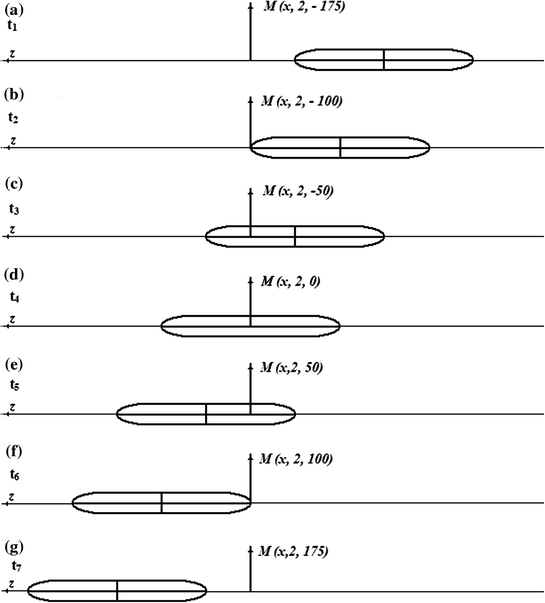

  

  The location of a moving body in the meridional plane: a $t_{1}$; b $t_{2}$; c $t_{3}$; d $t_{4}$; e $t_{5}$; f $t_{6}$; g $t_{7}$

• 2. $t_{2}$, when the body overcomes 75.0 m and its origin coincides with the axis of coordinates (Fig. 11b);

• 3. $t_{3}$, when the body crosses 125.0 m, i.e. ¼ part of its length and origin coincides with ¼ part of the body (Fig. 11c);

• 4. $t_{4}$, when the body crosses 175.0 m, i.e. ¼ part of its length and origin coincides with the center of the body (Fig. 11d);

• 5. $t_{5}$, when the body overcomes 225.0 m, i.e. ¾ part of its length and the origin of coordinates coincides with ¾ part of the body (Fig. 11e);

• 6. $t_{6}$, when the body overcomes 275.0 m, i.e. its entire length and origin coincide with the end (the tail part of the train) of the body (Fig. 11f);

• 7. $t_{7}$, when the body crosses 75.0 m and the origin is at a distance of 75.0 m behind the end (the tail part of the train) of the body (Fig. 11g).

Calculations of the velocity vector module $V = \sqrt {v_{x}^{2} + v_{y}^{2} + v_{z}^{2} }$ (theoretical) air flow caused by the movement of the body, for points located at a distance of 3.55, 6.00, 8.0, 10 m at $y = 0$ from the axis of the moving body (high-speed train) were carried out for the case. When the body moves at a constant speed (160, 200, 250, 350, 400 km/h) at altitude $h = 2\;{\text{m}}$ from the surface of the earth.

The speed of the air flow formed by the movement of the body, for points located at a distance of 3.55, 6.00, 8.0 and 10 m from the axis of the moving body (high-speed train), is determined by formula (9). Based on the results of calculations using information technologies, graphs are constructed of the change in the velocity of the air flow along a moving body at different distances from it (Figs. 12 and 13).

Fig. 12

Graphs of the change in the speed of the air flow along the moving body with a view of the head and tail parts in the form of a cone at a distance: 1–3.55 m; 2–6.0 m; 3–8.0 m; 4–10 m

Fig. 13

The graphs of the change in the speed of the air flow along the moving body with the appearance of the head and tail parts in the form came to life at a distance: 1–3.55 m; 2–6.0 m; 3–8.0 m; 4–10 m

As an example, Fig. 14 shows the graphs for the speed of 200 km/h.

Fig. 14

Modification of the velocity vector of the air flow V(m/s) as a function of the position of the moving body at the point “M” at various distances from it 1–3.55 m; 2–6.0 m; 3–8.0 m; 4–10.0 m

Analysis of the airflow velocity along the moving body at a speed of 200 km/h (Fig. 14) shows that the general nature of the graphs for velocities of 160, 200, 250, 350, 400 km/h is identical. As the moving body approaches, there is a slight perturbation of the air environment (zone I, Fig. 14).

The local maximum airflow velocity Vmax 1, that is, the maximum airflow velocity at the observation point M, located at a different distance from the moving body, reaches when the beginning of the moving body is located along the line connecting it with the observation point M (zone II, Fig. 14).

In the middle of the train, an extreme minimum air speed is required (zone III, Fig. 14).

The impulsive growth of velocity with an extremum of maximum Vmax 2 is observed when the end of the moving body is opposite point M (zone IV, Fig. 14).

After the passage of the point M, a gradual attenuation of the airflow velocity occurs (zone V, Fig. 14).

It should be noted that starting from the point A corresponding to the section AA in Fig. 14, while preserving its absolute value, the velocity vector changes in the opposite direction.

For example, at the point located at a distance of 3.55, 6, 8 and 10 m from the axis of the moving body (high-speed train) at a speed of 350 km/h, the maximum air speed is 41.5, 32.0, 26.2, 21.3 m/s (Figs. 11 and 12). At the points located at a distance of 3.55, 6, 8 and 10 m from the axis of the body moving at a speed of 200 km/h, the maximum speed of the air flow is respectively 21.4, 15.0, 10.5, 7.7 m/s.

Thus, the examination of a train as an axisymmetric body made it possible to obtain information revealing the features of the distribution of the air flow along and in the direction perpendicular from the axis of the moving train, and also the aerodynamic impact on the railway infrastructure objects and people [27, 29,30,31].

The resulting air flows have a negative impact on the environment, worsening the safe functioning of the system “high-speed railway—the environment (or surrounding objects)”.

Providing traffic safety for trains and passengers; uninterrupted operation of the entire infrastructure of a high-speed railway is the main condition for the organization of high-speed and high-speed passenger train traffic. A high degree of security is usually provided at all stages of creating a high-speed highway, i.e. is laid during the design, is provided during construction and is realized during the operation of the infrastructure of high-speed railways. This task is relevant in the design of high-speed train traffic on existing railways, which were designed for the maximum speed of passenger trains of 120–160 km/h.

Since, on existing lines, high-speed traffic is possible after a large-scale reconstruction and modernization of permanent facilities and structures of the existing infrastructure, in designing the organization of high-speed traffic using the existing railway infrastructure, the maximum permissible speeds for a high-speed train for each facility should be set separately their technical condition.

To ensure the safe operation of a high-speed railway, it is necessary to consider the aerodynamic impact on people and railway infrastructure objects as one of the main safety criteria for high-speed passenger train traffic, since a train moving at high speed has an aerodynamic effect on each object of magnitude. The technical condition of the object allows it to perceive the impact with the maximum permissible value without reducing the safety level of high-speed trains.

In connection with the above, in order to ensure the safe operation of a high-speed railway at all facilities or structural elements of the existing path infrastructure must be condition.

$$ P_{\hbox{max} \,i} \le P_{permi} , $$

(13)

where $P_{\hbox{max} \,i}$ maximum pressure on the object; $P_{permi}$ the maximum permissible value of an pressure that a given object can perceive.

Since, according to Bernoulli’s law, the aerodynamic pressure varies directly in proportion to the speed of the air flow $V_{f}$ created by the movement of the high-speed train, let us consider the theoretical aspects of establishing the value of the maximum train speed ensuring the fulfillment of condition (13).

The aerodynamic impact, strength and directivity of pressure on an object depend on the maximum speed and duration of the air flow, the spatial location, availability and proximity of the railway infrastructure objects relative to a moving high-speed train.

For each object i (or its constructive element) of the infrastructure of the existing railway, it is possible to draw up a design scheme of the effect of aerodynamic pressure on it (Fig. 15).

Fig. 15

Calculation schemes for the location of a high-speed train and objects: a train-object; b train-man-object; c train–worker; d train-passenger on a high platform-object; d train-passenger on a high platform-train; e train-passenger on a low platform-object; g train-passenger on a low platform-train

In all calculation cases, B for a known distance from a moving high-speed train to an object and the maximum permissible value of an impact that a given object can perceive, it is necessary to determine the speed of a high-speed train $V_{\hbox{max} \,i}$ and hence the airflow $V_{f}$ velocity that satisfies condition (13).

Thus, the problem of determining the aerodynamic effect on an i object is reduced to determining the velocity of the secondary airflow directly at the ith object when the high-speed train moves at a speed $V_{\hbox{max} \,i}$.

As the development of previously completed studies for a single solid body, the distribution of the air flow and the determination of its velocity along a moving high-speed train, was investigated on a model of a train consisting of a locomotive and 2n wagons [29].

To simplify the calculations, it is assumed that the locomotive and all cars in the cross section have the same shape, i.e. consist of a circular cylinder with identical head and tail shapes in the form of cones (Fig. 16).

Fig. 16

Scheme of high-speed train with locomotive and wagons 2n

The axisymmetric wave equation of the aerodynamic field near a high-speed train consisting of a locomotive and 2n wagons, can be decided as for a train consisting of one single wagon [30, 31]. In this case, the function $f(z)$ for each car can be represented in the form $f_{ij} (z)$, where the index i indicates the serial number of the wagon from the center of the train ($i = 0$ corresponds to the number of the middle car), the index j on the geometric shape of a part of the cars. If we assume that the car consists of three geometric shapes, then $j = 1,2,3$ ($j = 1$ corresponds to the cylindrical part, $j = 2$ tail section, $j = 3$ the head).

The propagation of an acoustic wave in the air can be represented by Eq. (7) with the boundary conditions (8) and (10) [24, 27]. The condition that the component along the axis 0y the velocity of the particles of the medium at the boundary of the half-space, in contrast to Eq. (9) [27, 29], takes the following form

$$ \frac{{\partial \varphi_{1} }}{\partial y} = 0\quad {\text{at}}\;y = - h - R - f(z). $$

(14)

To find the solution of the equation, the method of sources was used [28]. Considering the function $\varphi (r,z)$ satisfying Eq. (2), the boundary conditions (8) and (10) [29], the solution of Eq. (14), can be represented in the form

$$ \varphi_{1} = - \frac{1}{4\pi }\int\limits_{ - (2n + 1)L}^{(2n + 1)L} {\frac{q(\xi )\,d\xi }{{\sqrt {(\xi - z)^{2} + \alpha^{2} r^{2} } }}} , $$

(15)

where $q(z)$—the power of a source distributed over the surface of a moving body within $0 < r < f_{ij} (z),\; - (2n + 1)L < z < (2n + 1)L$.

For an axisymmetric body from formula (15) to [27], we can state that

$$ \frac{{\partial \varphi_{1} }}{\partial r} \to \frac{q(z)}{2\pi r}\quad {\text{at}}\;r \to 0. $$

(16)

Since, the problem is symmetric about the axis 0z, high-speed train consists of a locomotive and 2n the equation of the surface of the body $r = f_{ij} (z)$, as well as the power of the source $q(z)$ from each car and its components can be recorded separately.

For the cylindrical part of the car: at $2nL - L_{0} < z < 2nL + L_{0}$ and $(2nL + L_{0} ) < z < - (2nL - L_{0} )\;f_{n1} = R,\,q = 0$.

For the head and tail parts of the wagon located up to the middle of the train:

• at $\quad \begin{array}{*{20}l} {2nL + L_{0} < z < (2n + 1)L} \hfill & {f_{n2} = \gamma_{0} [(2n + 1)L - z],} \hfill \\ {q = - 2\pi v_{0} \gamma_{0}^{2} f_{n,2} ;} \hfill & {} \hfill \\ \end{array}$

• and $\quad \begin{array}{*{20}l} { - (2n + 1)L < z < - (2nL + L_{0} )} \hfill & {f_{n2} = \gamma_{0} [(2n + 1)L + z],} \hfill \\ {q = 2\pi v_{0} \gamma_{0}^{2} f_{n,2} .} \hfill & {} \hfill \\ \end{array}$

For the head and tail parts of the wagon located behind the middle of the train:

• at $\quad \begin{array}{*{20}l} {(2n + 1)L < z < (2n + 1)L + L_{0} } \hfill & {f_{n3} = \gamma_{0} [z - (2n + 1)L]} \hfill \\ {q = - 2\pi v_{0} \gamma_{0}^{2} f_{n3} ;} \hfill & {} \hfill \\ \end{array}$

• and $\quad \begin{array}{*{20}l} { - [(2n + 1)L + L_{0} [ < z < - (2n + 1)L} \hfill & {f_{n3} = - \gamma_{0} [(2n + 1)L + z]} \hfill \\ {q = - 2\pi v_{0} \gamma_{0}^{2} f_{n,3} .} \hfill & {} \hfill \\ \end{array}$

For example, for a car $i = 1$ and its parts $j = 2$ as:

$$ 2L + L_{0} < z < 3L;\;f_{12} = \gamma_{0} (3L - z);\;q = - 2\pi v_{0} \gamma_{0}^{2} f_{12} $$

Taking into account the symmetry of the problem with respect to the variable z, power source from each car and its components $q(z)$, Eq. (15) can be represented in the following form

$$ \begin{aligned} \varphi_{1} & = - \frac{{v_{0} \gamma_{0}^{2} }}{2}\left\{ {\sum\limits_{i = 0}^{n} {\left[ {\int\limits_{{2iL + L_{0} }}^{(2i + 1)L} {\frac{(2i + 1)L - \xi }{{\sqrt {(z + \xi )^{2} + \alpha^{2} r^{2} } }}} \,d\xi - \int\limits_{{2iL + L_{0} }}^{(2i + 1)L} {\frac{(2i + 1)L - \xi }{{\sqrt {(z - \xi ) + \alpha^{2} r^{2} } }}d\xi } } \right]} } \right\} \\ & \quad + \frac{{v_{0} \gamma_{0}^{2} }}{2}\left\{ {\sum\limits_{i = 1}^{n} {\left[ {\int\limits_{(2i - 1)L}^{{2iL - L_{0} }} {\frac{\xi - (2i - 1)L}{{\sqrt {(z + \xi )^{2} + \alpha^{2} r^{2} } }}} \,d\xi - \int\limits_{(2i - 1)L}^{{2iL - L_{0} }} {\frac{\xi - (2i - 1)L}{{\sqrt {(z - \xi ) + \alpha^{2} r^{2} } }}} d\xi } \right]} } \right\}. \\ \end{aligned} $$

(17)

Introducing the variable $r_{ij} = r_{ij} (x,y,z)$ expressed by the formula

$$ r_{ij} = \sqrt {x^{2} + \left[ {2f_{ij} (z) + 2h + 2R + y} \right]^{2} } . $$

(18)

The total potential presented in the form

$$ \varphi_{n} = \varphi_{1} (r,z) + \varphi_{1} [r_{ij} (x,y,z),z]. $$

(19)

Function $\varphi_{n} (x,y,z)$ satisfies the boundary condition (14), the function $\varphi_{1} = \varphi_{1} [r_{ij} (x,y,z),z]$ satisfies Eq. (16) only when $\gamma_{0} = 0$. Assuming $\gamma_{0}$ a small parameter and setting $f_{ij} = \gamma_{0} f_{0ij}$ functions $1/r_{ij} = 1/\sqrt {x^{2} + \left[ {2\gamma_{0} \,f_{0ij} (z) + 2h + 2R + y} \right]^{2} }$ can be expanded in powers of this parameter as

$$ \frac{1}{{r_{ij} }} = \frac{1}{{\sqrt {x^{2} + \left[ {2\gamma_{0} \,f_{0ij} (z) + 2h + y} \right]^{2} } }} = \frac{1}{{r_{1} }} + \gamma_{0} \frac{{2(2h + y)f_{0ij} (z)}}{{r_{1}^{3} }} + \cdots $$

(20)

where $r_{1} = \sqrt {x^{2} + (2h + 2R + y)^{2} }$.

If we substitute expression (20) into (17), then formula (19) takes the form

$$ \varphi_{n} = \gamma_{0}^{2} \left[ {\varphi_{01} (r,z) + \varphi_{01} (r_{1} ,z) + \gamma_{0} \varphi_{02} + \cdots } \right], $$

(21)

where

$$ \begin{aligned} \varphi_{01} & = - \frac{{v_{0} }}{2}\left\{ {\sum\limits_{i = 0}^{n} {\left[ {\int\limits_{{2iL + L_{0} }}^{(2i + 1)L} {\frac{(2i + 1)L - \xi }{{\sqrt {(z + \xi )^{2} + \alpha^{2} r^{2} } }}} \,d\xi - \int\limits_{{2iL + L_{0} }}^{(2i + 1)L} {\frac{(2i + 1)L - \xi }{{\sqrt {(z - \xi ) + \alpha^{2} r^{2} } }}\,d\xi } } \right]} } \right\} \\ & \quad + \frac{{v_{0} }}{2}\left\{ {\sum\limits_{i = 1}^{n} {\left[ {\int\limits_{(2i - 1)L}^{{2iL - L_{0} }} {\frac{\xi - (2i - 1)L}{{\sqrt {(z + \xi )^{2} + \alpha^{2} r^{2} } }}} \,d\xi - \int\limits_{(2i - 1)L}^{{2iL - L_{0} }} {\frac{\xi - (2i - 1)L}{{\sqrt {(z - \xi ) + \alpha^{2} r^{2} } }}} \,d\xi } \right]} } \right\} \\ \end{aligned} $$

(22)

$$ \begin{aligned} \phi _{{02}} & = v_{0} \left\{ {\sum\limits_{{i = 0}}^{n} {\left[ \begin{gathered} \int\limits_{{2iL + L_{0} }}^{{(2i + 1)L}} {\frac{{[(2i + 1)L - \xi ](2h + y]f_{{0ij}} (z)}}{{\sqrt {[\{ (z + \xi )^{2} + \alpha ^{2} r_{1}^{2} ]^{3} } }}d\xi } \hfill \\ \quad - \int\limits_{{2iL + L_{0} }}^{{(2i + 1)L}} {\frac{{[(2i + 1)L - \xi ][2h + y]f_{{0ij}} (z)}}{{\sqrt {][z - \xi ) + \alpha ^{2} r_{1}^{2} ]^{3} } }}d\xi } \hfill \\ \end{gathered} \right]} } \right\} \\ & \quad + v_{0} \left\{ {\sum\limits_{{i = 1}}^{n} {\left[ \begin{gathered} \int\limits_{{(2i - 1)L}}^{{2iL - L_{0} }} {\frac{{[\xi - (2i - 1)L][2h + y]f_{{0ij}} (z)}}{{\sqrt {[(z + \xi )^{2} + \alpha ^{2} r_{1}^{2} ]^{3} } }}d\xi } \hfill \\ \quad - \int\limits_{{(2i - 1)L}}^{{2iL - L_{0} }} {\frac{{[\xi - (2i - 1)L][2h + y]f_{{0ij}} (z)}}{{\sqrt {[(z - \xi ) + \alpha ^{2} r_{1}^{2} } ]^{3} }}} d\xi \hfill \\ \end{gathered} \right]} } \right\} \\ \end{aligned} $$

(23)

In the sum of the potentials (21), the first approximation is the function $\varphi_{01}$, which satisfies Eq. (7) [27, 29] and the boundary condition (14).

The components of the velocity vector of air particles can be determined by the following formulas at $\gamma_{0}^{3} \approx 0$:

$$ \begin{aligned} \frac{{\partial \varphi_{n} }}{\partial x} & = \gamma_{0}^{2} (\frac{{\partial \varphi_{01} (r,z)}}{\partial r}\frac{\partial r}{\partial x} + \frac{{\partial \varphi_{01} (r_{1} ,z)}}{{\partial r_{1} }}\frac{{\partial r_{1} }}{\partial x}) \\ & = \gamma_{0}^{2} \frac{{v_{0} x}}{2r}\left\{ {\sum\limits_{i = 0}^{n} {\left[ {\int\limits_{{2iL + L_{0} }}^{(2i + 1)L} {\frac{(2i + 1)L - \xi }{{(z + \xi )^{2} + \alpha^{2} r^{2} }}} \,d\xi - \int\limits_{{2iL + L_{0} }}^{(2i + 1)L} {\frac{(2i + 1)L - \xi }{{(z - \xi )^{2} + \alpha^{2} r^{2} }}\,d\xi } } \right]} } \right\} \\ & \quad - \gamma_{0}^{2} \frac{{v_{0} x}}{2r}\left\{ {\sum\limits_{i = 1}^{n} {\left[ {\int\limits_{(2i - 1)L}^{{2iL - L_{0} }} {\frac{\xi - (2i + 1)L}{{(z + \xi )^{2} + \alpha^{2} r^{2} }}} \,d\xi - \int\limits_{(2i - 1)L}^{{2iL - L_{0} }} {\frac{\xi - (2i - 1)L}{{(z - \xi )^{2} + \alpha^{2} r^{2} }}\,d\xi } } \right]} } \right\} \\ & \quad + \gamma_{0}^{2} \frac{{v_{0} x}}{{2r_{1} }}\left\{ {\sum\limits_{i = 0}^{n} {\left[ {\int\limits_{{2iL + L_{0} }}^{(2i + 1)L} {\frac{(2i + 1)L - \xi }{{(z + \xi )^{2} + \alpha^{2} r_{1}^{2} }}} \,d\xi - \int\limits_{{2iL + L_{0} }}^{(2i + 1)L} {\frac{(2i + 1)L - \xi }{{(z - \xi )^{2} + \alpha^{2} r_{1}^{2} }}\,d\xi } } \right]} } \right\} \\ & \quad - \gamma_{0}^{2} \frac{{v_{0} x}}{{2r_{1} }}\left\{ {\sum\limits_{i = 1}^{n} {\left[ {\int\limits_{(2i - 1)L}^{{2iL - L_{0} }} {\frac{\xi - (2i - 1)L}{{(z + \xi )^{2} + \alpha^{2} r_{1}^{2} }}} \,d\xi - \int\limits_{(2i - 1)L}^{{2iL - L_{0} }} {\frac{\xi - (2i + 1)L}{{(z - \xi )^{2} + \alpha^{2} r_{1}^{2} }}\,d\xi } } \right]} } \right\} \\ \end{aligned} $$

(24)

$$ \begin{aligned} \frac{{\partial \varphi_{n} }}{\partial y} & = \gamma_{0}^{2} (\frac{{\partial \varphi_{01} (r,z)}}{\partial r}\frac{\partial r}{\partial y} + \frac{{\partial \varphi_{01} (r_{1} ,z)}}{{\partial r_{1} }}\frac{{\partial r_{1} }}{\partial y}) \\ & = \gamma_{0}^{2} \frac{{v_{0} y}}{2r}\left\{ {\sum\limits_{i = 0}^{n} {\left[ {\int\limits_{{2iL + L_{0} }}^{(2i + 1)L} {\frac{(2i + 1)L - \xi }{{(z + \xi )^{2} + \alpha^{2} r^{2} }}} \,d\xi - \int\limits_{{2iL + L_{0} }}^{(2i + 1)L} {\frac{(2i + 1)L - \xi }{{(z - \xi )^{2} + \alpha^{2} r^{2} }}\,d\xi } } \right]} } \right\} \\ & \quad - \gamma_{0}^{2} \frac{{v_{0} y}}{2r}\left\{ {\sum\limits_{i = 1}^{n} {\left[ {\int\limits_{(2i - 1)L}^{{2iL - L_{0} }} {\frac{\xi - (2i + 1)L}{{(z + \xi )^{2} + \alpha^{2} r^{2} }}} \,d\xi - \int\limits_{(2i - 1)L}^{{2iL - L_{0} }} {\frac{\xi - (2i - 1)L}{{(z - \xi )^{2} + \alpha^{2} r^{2} }}\,d\xi } } \right]} } \right\} \\ & \quad + \gamma_{0}^{2} \frac{{v_{0} (y + 2h + 2R)}}{{2r_{1} }}\left\{ {\sum\limits_{i = 0}^{n} {\left[ {\int\limits_{{2iL + L_{0} }}^{(2i + 1)L} {\frac{(2i + 1)L - \xi }{{(z + \xi )^{2} + \alpha^{2} r_{1}^{2} }}} \,d\xi - \int\limits_{{2iL + L_{0} }}^{(2i + 1)L} {\frac{(2i + 1)L - \xi }{{(z - \xi )^{2} + \alpha^{2} r_{1}^{2} }}\,d\xi } } \right]} } \right\} \\ & \quad - \gamma_{0}^{2} \frac{{v_{0} (y + 2h + 2R)}}{{2r_{1} }}\left\{ {\sum\limits_{i = 1}^{n} {\left[ {\int\limits_{(2i - 1)L}^{{2iL - L_{0} }} {\frac{\xi - (2i - 1)L}{{(z + \xi )^{2} + \alpha^{2} r_{1}^{2} }}} \,d\xi - \int\limits_{(2i - 1)L}^{{2iL - L_{0} }} {\frac{\xi - (2i - 1)L}{{(z - \xi )^{2} + \alpha^{2} r_{1}^{2} }}\,d\xi } } \right]} } \right\} \\ \end{aligned} $$

(25)

$$ \begin{aligned} \frac{{\partial \varphi_{n} }}{\partial z} & = \gamma_{0}^{2} (\frac{{\partial \varphi_{01} (r,z)}}{\partial z} + \frac{{\partial \varphi_{01} (r_{1} ,z)}}{\partial z}) \\ & = \gamma_{9}^{2} \frac{{v_{0} }}{2}\left\{ {\sum\limits_{i = 0}^{n} {\left[ {\int\limits_{{2iL + L_{0} }}^{(2i + 1)L} {\frac{[(2i + 1)L - \xi ](z + \xi )}{{(z + \xi )^{2} + \alpha^{2} r^{2} }}} \,d\xi - \int\limits_{{2iL + L_{0} }}^{(2i + 1)L} {\frac{[(2i + 1)L - \xi ](z - \xi )}{{(z - \xi )^{2} + \alpha^{2} r^{2} }}\,d\xi } } \right]} } \right\} \\ & \quad - \gamma_{0}^{2} \frac{{v_{0} }}{2}\left\{ {\sum\limits_{i = 1}^{n} {\left[ {\int\limits_{(2i - 1)L}^{{2iL - L_{0} }} {\frac{[\xi - (2i - 1)L](z + \xi )}{{(z + \xi )^{2} + \alpha^{2} r^{2} }}} \,d\xi - \int\limits_{(2i - 1)L}^{{2iL - L_{0} }} {\frac{[\xi - (2i - 1)L](z - \xi )}{{(z - \xi )^{2} + \alpha^{2} r^{2} }}\,d\xi } } \right]} } \right\} \\ & \quad - \gamma_{0}^{2} \frac{{v_{0} }}{2}\left\{ {\sum\limits_{i = 0}^{n} {\left[ {\int\limits_{{2iL + L_{0} }}^{(2i + 1)L} {\frac{[(2i + 1)L - \xi ](z + \xi )}{{(z + \xi )^{2} + \alpha^{2} r_{1}^{2} }}} \,d\xi - \int\limits_{{2iL + L_{0} }}^{(2i + 1)L} {\frac{[(2i + 1)L - \xi ](z - \xi )}{{(z - \xi )^{2} + \alpha^{2} r_{1}^{2} }}\,d\xi } } \right]} } \right\} \\ & \quad - \gamma_{0}^{2} \frac{{v_{0} }}{2}\left\{ {\sum\limits_{i = 1}^{n} {\left[ {\int\limits_{(2i - 1)L}^{{2iL - L_{0} }} {\frac{[\xi - (2i - 1)L](z + \xi )}{{(z + \xi )^{2} + \alpha^{2} r_{1}^{2} }}} \,d\xi - \int\limits_{(2i - 1)L}^{{2iL - L_{0} }} {\frac{[\xi - (2i - 1)L](z - \xi )}{{(z - \xi )^{2} + \alpha^{2} r_{1}^{2} }}\,d\xi } } \right]} } \right\} \\ \end{aligned} $$

(26)

Absolute speed of air flow generated by the system of high-speed train cars when it moves with a steady speed at an arbitrary point M(x, y, z) can be defined as

$$ v = \sqrt {v_{x}^{2} + v_{y}^{2} + v_{z}^{2} } . $$

(27)

The air flow pressure can be determined from the formula

$$ \Delta p = - \rho_{0} \frac{{\partial \varphi_{n} }}{\partial t} = \rho_{0} v_{0} \gamma_{0}^{2} \left[ {\frac{{\partial \varphi_{01} (r,z)}}{\partial z} + \frac{{\partial \varphi_{01} (r_{1} ,z)}}{\partial z}} \right]. $$

(28)

In Fig. 17 airs of change in airflow. In calculations it is accepted $L = 25\;{\text{m}},L_{0} = 20\;{\text{m}}$, $R = 2\;{\text{m}},v_{0} = 200\;{\text{km}}/{\text{h}}$, $\rho_{0} = 1.2\;{\text{kg/m}}^{3} ,\gamma_{0} = 0.4$.

Fig. 17

Graphs of the change in aerodynamic airflow pressure versus time: a with closed and b open between car spaces

A comparison of the calculation results with the experimental data obtained in [16, 32] shows their qualitative agreement, the quantitative difference is 1.5–2.5 times. This difference can be explained by the fact that in the accepted calculation model the train is represented in the form of a long whole axisymmetric body whose initial and terminal sections have a kind of revived. The air is received by a compressible ideal gas, which is an essential approximation of the circuit to the real situation. In reality, the speed of the air flow is largely influenced by the shape of the moving train, the additional air flow arising in the space between the cars, and also the phenomenon of turbulence in the flow near a moving train. To take into account these factors, the correction factors can be introduced into the calculation formulas by the value of the airflow velocity.

Analysis of the graphs shows that in both cases the negative pressure is greater than the positive one. The reliability of these calculations is confirmed by the results of earlier experiments in the USA, Russia, Sweden [32, 33]. The effect between the car space on the magnitude of the negative (suction) aerodynamic pressure is clearly visible in the graph shown in Fig. 16b. On the railways of individual states, the movement of dual high-speed trains is practiced. With sufficient streamlining of the head and tail wagons, in places the pairing of trains produces a negative aerodynamic pressure, the value of which considerably exceeds the value of the excess pressure. Similar graphs can be constructed for other velocities and distances.

Thus, it can be argued that in order to ensure the safe operation of the railway infrastructure, it is necessary to take into account aerodynamic flows and pressures, regardless of their orientation. Using the results of calculations, it is also possible to construct a curve for the dependence of the magnitude of the aerodynamic pressure on the speed of trains and the distance to the point under consideration $P_{\hbox{max} } = f(V_{\hbox{max} } ,B)$ (Fig. 18). With the help of these dependencies, it is possible to set the maximum permissible speed of passage of a high-speed train along the object.

Fig. 18

Graphs of change in aerodynamic pressure

As an example, solutions of the problems most often encountered in the practice of designing the high-speed movement of passenger trains, whose calculated schemes are shown in Fig. 15, are considered.

Ensuring the safety of passengers on the platform and workers of the railway in the immediate vicinity of the passing high-speed train is an actual task in connection with the current change in the aerodynamic field, due to the involvement of the air mass in motion, the speed of which and the pressure created depend on the speed and geometry of the high-speed train, the presence of the surrounding railway infrastructure facilities.

The strength of the impact on people and infrastructure depends not only on the maximum speed of the air flow, but also on its duration, location relative to the moving train, which should be considered as one of the main safety criteria. So far, the studies have been empirical. In particular, experiments conducted in Japan, France, Germany, the United States, Russia and other countries have experimentally established airspeed rates, the value of aerodynamic pressure around a high-speed train; its impact on people on the passenger platform and the construction of railway infrastructure facilities. Theoretically, the issue has not been studied enough.

For this purpose, an attempt was made to develop a design scheme with the following boundary conditions: a passenger platform of the “coastal” type adjoins, the passenger building; the edge of the platform is at a distance $b_{\hbox{min} }$ from the axis of the path; The height of the platform is h (Fig. 15c); the passenger is on a platform width $B_{\hbox{min} }$ on distance $b_{1\hbox{min} }$ from the axis of the fence and distance $b_{2\hbox{min} }$ from the passenger building; distance from the track axis to the edge of the platform $b_{\hbox{min} }$ and platform height h are dimensioned “C₂₅₀” [8, 9]; a person is affected by force F, axial x and perpendicular to the vertical axis of the person. We can assume, since the surface (area) of the person on the platform is constant, the value of the force F, apparently varies directly in proportion to the value of the aerodynamic pressure P, formed during the passage of a high-speed train.

It is also clear that to ensure the safety of the person on the platform, the actual pressure on it should not exceed the regulatory threshold

$$ P_{f} \le P_{n} $$

(29)

where

$P_{f}$ :

the actual (excess) pressure (air flow) per person, Pa;

$P_{n}$ :

the value of permissible pressure, regulated by the sanitary norms of the country, Pa.

For practical purposes, it is important to determine the point “M” with the coordinates M (x, y, z) where condition (29).

If a person is on a platform in a stationary state, at some point “M” his coordinates can be represented in the form $M(b_{1\hbox{min} } ,y,z)$. In this case $x = b_{1\hbox{min} } ,\,y = const,\,z = const$ (Fig. 19).

Fig. 19

The layout of the person (passenger) on the high coastal platform: a in plan, b in cross section

According to the Bernoulli law, the aerodynamic pressure is derived from the aerodynamic flow

$$ \Delta P = \frac{{v^{2} \rho }}{2}. $$

(30)

From where you can determine the maximum value of the air speed

$$ v_{\hbox{max} .additional} = \sqrt {\frac{{2\Delta P_{n} }}{\rho }} . $$

(31)

Thus, the solution of the problem reduces to determining the minimum distance $b_{1\hbox{min} }$ or points $M(b_{1\hbox{min} } ,y,z)$, where the maximum value of air speed reaches $v_{\hbox{max} .additional}$ and condition (29).

Based on the results of previous calculations, graphs of the dependence of the maximum airflow velocity on the remoteness of the considered observation point can also be constructed (Fig. 20).

Fig. 20

The graph of the maximum airflow velocity versus the distance of the observed point of observation

The resulting graphs allow us to establish:

• the minimum distance $b_{1\hbox{min} }$, where the maximum values of the airflow velocity are equal $v_{\hbox{max} .additional}$;

• minimum width of the passenger platform $B_{\hbox{min} }$ on sections of high-speed trains;

• the maximum speed of passage of high-speed passenger trains at the station (a detour) along a high passenger platform with a known width.

In all cases, the condition (29) is satisfied.

Let us assume that the maximum permissible pressure value regulated by sanitary norms is equal to $P_{n} = 100\,{\text{Pa}}$. According to the formula (31), the values of the maximum airflow velocity $v_{\hbox{max} .additional}$, which is 12.9 m/s, which corresponds to a distance of 4.44 m (Fig. 20). The maximum pressure on a person in a stationary state (standing still) at a distance $b_{1\hbox{min} } \ge 4.44\;{\text{m}}$ from the axis of the moving body with a speed of 160 km/h to make no more than 100 Pa, which corresponds to the sanitary standards.

The above methodology also allows one to investigate the effects of secondary air streams, formed by high-speed passenger trains, on the surrounding environment along the high-speed railway.

In the republics of Central Asia and Kazakhstan, about 3000 km of railways built in the sand desert zone are constantly exposed to sand drifts and are operated in extremely difficult conditions.

Currently, the Bukhara-Miskin line is being built, designed in the future to organize high-speed traffic through Urgench to Khiva station and separately from Miskin to Nukus station. The railway from Bukhara to Miskin crosses the massifs of the sands of southern Kyzylkum (Fig. 21).

Fig. 21

The scheme of the Bukhara-Miskin railway

These sands with a wind speed on the surface of the sand more critical (>4.1 m/s) come into motion and with a further increase in speed are transferred and create mobile forms of relief. This creates problems both during the construction period and during the operation of the railway. In particular, the roadbed is blown out, the drainage structures and the top structure of the road are filled up.

In the course of construction technogenic sands are formed, losing their natural composition and structure. As a result, technogenic sands grow after 6–8 years [34, 35].

When introducing high-speed traffic of passenger trains on this section, unlike other routes, additional questions arise that require their scientific and technical solutions. These include ensuring the stable operation of the roadbed, securing the slopes of the roadbed erected from sand-dune and the roadside strip.

The technology of construction and strengthening of the roadbed erected from sand-dune, fixing its slopes and adjacent to the railroad tracks are devoted to the work of A.I. Adylkhodzhaev, R.S Zakirov, M.M. Mirakhmedov, T.I. Fazylov and other scientists [34,35,36,37,38]. They also proposed various ways to protect the way from sand drifts and methods of fixing sand-dune carried by the wind.

In this study, the possibility of sand deflation of the adjacent strip, embankment slopes and excavation by a secondary airflow—a stream formed from the movement of a high-speed train—is considered.

The theoretical premise can be the transition of a grain of sand from a state of rest to a motion which, in the prevailing case, occurs at air flow velocities above 4.1 m/s, called critical. Above this threshold, the sand grains come into motion, at the beginning, by sliding, rolling, then spasmodically and in a suspended state.

The main form of motion is a jump, the parameters of which depend both on the size and shape of the sand, and the structure of the wind-sand flow, formed by the wind speed, in this case on the speed of the air flow created by the moving high-speed train. the negative impact of which on the state of the environment in the sand desert area should be included in the high-speed railway project. As measures, the following organizational and technical measures may be envisaged:

• (1) fixation of susceptible sands:

• (2) in the body of the roadbed;

• (3) on the slopes of the roadbed;

• (4) on the adjacent strip of width B (m);

• (5) limiting the speed of the movement of high-speed trains to a level where the speed of the air flow created by them will be equal to or less than the critical one, i.e.

  $$ v_{af} \le v_{cr} $$

  (32)

The technology of erecting a roadbed from sand-dune, reinforcing the roadbed, fixing its slopes and adjacent to the railroad tracks are not the subject of this research.

Thus, the issue of selection and justification of measures preventing the negative impact of the movement of a high-speed train on the state of the environment in the area of sandy deserts is reduced to establishing:

• 1. Point locations $n_{i}$ on the surface of the earth with coordinates $(x_{i} ,y_{i} ,z_{i} )$, where condition (32), those at a known value of the speed of the distance train $(x_{i} ,y_{i} ,z_{i} )$.

• 2. Train speeds $v_{ni}$ at the point $n_{i} (x_{i} ,y_{i} ,z_{i} )$ on the surface of the earth, under which condition (32), those at a certain value of the physical and mechanical properties of the soil at the point $n_{i}$ speeds $v_{ni}$.

In both cases, in order to solve the problem, it is necessary to establish the velocity of the secondary airflow $v_{af}$, which can be established by expression (27). The speed of a high-speed train can be established by traction calculations.

Using the graph of the maximum air speed as a function of the remoteness of the observed observation point (without taking into account the correction factor), which is shown in the figure with a thick line (Fig. 22), the minimum distance from the axis of the path on which the sand fixing works should be established.

Fig. 22

The graph of the maximum airflow velocity versus the distance of the observed point of observation

These graphics allow:

• determine the nature of the distribution of air flow and determine its speed along a moving high-speed train;

• to build along the roadbed isolines with the same speed of air flow, formed by the movement of a high-speed train;

• establish the width of the strip of fastening work along the earthen canvas, sprinkled from sand-dune and exposed to wind-transported sands;

• optimize the amount of sand fixing work;

• choose the method (method) of fixing sand.

The results of the research can be used in the design of high-speed railways in the regions where loose sand is spread.

As a result of a complex of theoretical studies of the aerodynamics of a high-speed train, as an axisymmetric body moving in a compressible (acoustic) medium,

• 1. The nature of the distribution of the air flow and the speed along the moving high-speed train, as well as the velocity distribution along the roadbed (isolines with the same speed) of the air flow formed during the movement of the high-speed train.

• 2. The maximum permissible speed of a high-speed train, taking into account the technical condition of permanent devices and structures of the existing railway infrastructure.

• 3. Technical parameters of individual objects and structural elements of the infrastructure of high-speed railways subject to the effect of aerodynamic pressure for a given maximum speed of high-speed trains.

• 4. The width of the strip of the roadbed (including slopes, cuvettes) spilled from sand-dune and to be fixed with appropriate justification (covering with heavy soil, impregnation of astringent, shelter from geotextile in combination with hydroseeding) provided that the velocity of the secondary wind generated from movement high-speed train exceeds the critical, as well as the minimum required sand-consolidation work.

• 5. The places of installation of fences on the runways, preventing unauthorized access to people and animals, the minimum safe distance of people in the vicinity of the passing train in accordance with the requirements of the national standard.

• 6. Rationally use the land fund allocated for the construction of high-speed railways.

The proposed methodological approach can be used in the practice of organizing high-speed and high-speed train traffic, in particular, when designing it on existing and newly constructed railways.

4 The Combined Movement of Passenger and Freight Trains to High-Speed Sections of Existing Railways

As an alternative solution to high-speed traffic, consider the organization of high-speed passenger traffic on existing lines with the combined movement of freight and passenger trains.

The presence of combined cargo and passenger traffic, the tendency to a known increase in freight traffic, in the event of an actual depletion of capacity reserves, create serious additional difficulties when introducing high-speed train traffic on single-track lines.

The introduction into circulation of several high-speed trains can lead to premature exhaustion of the carrying capacity of single-track rail and road and the emergence of a “capacity deficit”. Therefore, the task of increasing the speed of passenger trains must be considered together with the task of eliminating the shortage of throughput and carrying capacity resulting from the accelerated removal of freight trains by accelerated passenger trains.

Let us assume that the required carrying capacity of a single-track section varies linearly, those

$$ G_{r} = G_{p} + a \cdot t $$

(33)

where,

${\text{G}}_{\text{p}}$ :

carrying capacity for the initial year of operation, mln.t.;

a :

the rate of annual growth in the required capacity, mln.t/year;

t :

billing year

Required carrying capacity ${\text{G}}_{\text{r}} = f(t)$ changing in time, as a rule, increases. Possible carrying capacity of the site up to $G_{p}^{t} = f(t)$ and after $G_{p}^{a} = f(t)$ the introduction of high-speed train traffic also varies with time. Since in most cases the dimensions of passenger traffic are increasing, the possible carrying capacity of the section decreases with time, i.e. curves ${\text{G}}_{p} = f(t)$ tend to decrease (Fig. 23).

Fig. 23

Graphs of possible and required carrying capacity

The graphical representation of the change in the required and possible carrying capacity (Fig. 23) shows that an increase in speed after modernization leads to a premature exhaustion of capacity for a period $\Delta {\text{t}}$, those, there is a shortage of carrying capacity $\Delta G$.

If the annual growth rate of the required capacity is known, then it is possible to establish a time limit $\Delta t$ for the premature exhaustion of the possible carrying capacity.

From the triangle ABC

$$ tg\,\alpha =\Delta G/\Delta t, $$

(34)

as

$$ tg\,\alpha = a, $$

(35)

then,

$$ \Delta t = a\Delta G. $$

(36)

The magnitude of the deficit of carrying capacity ΔG there is a difference in the possible carrying capacity of the site up to $G_{p}^{t} = f(t)$ and after $G_{p}^{a} = f(t)$ introduction of high-speed train traffic, those

$$ \Delta G = G_{p}^{t} - G_{p}^{a} $$

(37)

In turn, the possible carrying capacity of the site before $G_{p}^{t} = f(t)$ and after $G_{p}^{a} = f(t)$ putting into motion $N_{h - s}^{a}$ high-speed trains, respectively, can be defined as

$$ \begin{aligned} G_{p}^{t} & = \frac{{365 \cdot Q_{c} 10^{ - 6} }}{\gamma }N_{c}^{t} == \frac{{365Q_{c} 10^{ - 6} }}{\gamma } \\ & \quad \cdot \left\{ {\frac{{N_{p} }}{1 + \beta } - N_{pas}^{t} \varepsilon_{pas} - N_{as}^{t} (\varepsilon_{as} - 1) - N_{e}^{t} \varepsilon_{e} - N_{emp}^{t} } \right\} \\ \end{aligned} $$

(38)

$$ \begin{aligned} G_{p}^{a} & = \frac{{365 \cdot Q_{c} 10^{ - 6} }}{\gamma }N_{c}^{a} = = \frac{{365Q_{c} 10^{ - 6} }}{\gamma } \\ & \quad \cdot \left\{ {\frac{{N_{p} }}{1 + \beta } - N_{h - s}^{a} \varepsilon_{h - s} - N_{pas}^{a} \varepsilon_{pas} - N_{as}^{a} (\varepsilon_{as} - 1) - N_{e}^{a} \varepsilon_{e} - N_{emp}^{a} } \right\} \\ \end{aligned} $$

(38′)

The carrying capacity of the haulage in cargo traffic can be determined by the following formula [39]

$$ N_{c} = \left\{ {\frac{{N_{p} }}{1 + \beta } - N_{pas} \varepsilon_{pas} - N_{as} (\varepsilon_{as} - 1) - N_{e} \varepsilon_{e} - N_{emp} } \right\} $$

(39)

Introduction of high-speed (or high-speed) traffic of passenger trains $N_{h - s}^{a}$ on existing single-track lines can be carried out:

• 1. Due to newly introduced high-speed trains;

• 2. By transferring a number of existing trains into the category of high-speed trains.

In the second variant, the number of passenger trains after the transfer to the category of high-speed $N_{h - s}^{a}$ trains can be defined as,

$$ N_{pas}^{a} = N_{pas}^{t} - N_{h - s}^{a} $$

(40)

We assume that the number of prefabricated, economic, empty, accelerated freight trains before and after the introduction of high-speed traffic of passenger trains does not change. Substituting the expressions (38), (38′) and (40) into the formula (37) after some transformations, it is not difficult to establish the magnitude of the deficit of the carrying capacity $\Delta G$ after the introduction of high-speed traffic of passenger trains:

• with the introduction of newly high-speed trains

  $$ \Delta G = \frac{{365 \cdot Q_{c} 10^{ - 6} }}{\gamma }N_{h - s}^{a} \varepsilon_{h - s} $$

  (41)

• when moving $N_{h - s}^{a}$ the number of existing trains in the category of high-speed trains

  $$ \Delta G = \frac{{365 \cdot Q_{c} 10^{ - 6} }}{\gamma }N_{h - s}^{a} (\varepsilon_{h - s} - \varepsilon_{pas} ) $$

  (42)

Expression analysis (37), (41), (42) shows that the term of premature exhaustion of the possible carrying capacity $\Delta {\text{t}}$ directly depends on the number of high-speed trains $N_{h - s}^{a}$, ratio of speeds of high-speed and passenger trains $\varepsilon_{pas} ,\varepsilon_{h - s}$, as well as the rate of annual growth in the required carrying capacity—a.

Compensation of the deficit of carrying capacity resulting from the introduction of high-speed passenger train traffic on single-track sections is possible due to:

• 1. Increase in the norms of the mass of the train while maintaining the possible throughput ${\text{N}}_{{{\text{h}} - {\text{s}}}}^{\text{a}} ,\,{\text{N}}_{\text{p}}$;

• 2. Increase in possible bandwidth $N_{p}$ due to the transition to a smaller inter-train interval I on a single-track line.

In the first case, in order to preserve the possible carrying capacity before and after the introduction of the high-speed traffic of passenger trains, the condition

$$ G_{p}^{t} = G_{p}^{a} . $$

(43)

Thus equality (38) and (38′) can be written down in a following kind

$$ G_{p}^{t} = \frac{{365 \cdot Q_{c}^{t} 10^{ - 6} }}{\gamma }N_{c}^{t} , $$

(44)

$$ G_{p}^{a} = \frac{{365 \cdot Q_{c}^{a} 10^{ - 6} }}{\gamma }N_{c}^{a} . $$

(45)

Substituting (44), (45) into (43) and solving the resulting equation for $Q_{c}^{a}$

$$ Q_{c}^{a} = Q_{c}^{t} \frac{{N_{c}^{t} }}{{N_{c}^{a} }}. $$

(46)

The ratio of the number of freight trains before and after the introduction of high-speed trains will be denoted by

$$ k_{inc} = \frac{{N_{c}^{t} }}{{N_{c}^{a} }}. $$

(46′)

Then, Eq. (46) takes the following

$$ Q_{c}^{a} = Q_{c}^{t} k_{inc} , $$

(47)

where, $k_{inc}$—coefficient of increase in the mass of the freight train after the introduction of high-speed traffic of passenger trains.

Thus, to preserve the possible carrying capacity after the introduction of high-speed traffic $N_{h - s}^{a}$ passenger trains it is necessary to increase the mass of each freight train in accordance with (47) by the amount $k_{inc}$. The value of the weight increase coefficient of the composition depends on the quantity, the maximum speed of movement of high-speed trains in circulation, and also on the speed of freight trains. The graphical representation of the change in the values of the mass increase coefficient of the composition is shown in Fig. 24.

Fig. 24

Change in the value of the mass composition increase coefficient

Analysis of the results of the research shows that if in the section of a single-track railway in question passenger trains with speeds of up to 120, 140, 160 km/h were in circulation, then a sharp increase in the value of the conditional mass increase of the freight composition occurs when moving to higher speed levels. At speeds above 180 km/h, the value of the conditional coefficient of increase in the mass of the composition does not actually change, i.e. of the speed does not depend. To a large extent, it depends on the number of high-speed trains being introduced (or accelerated) and the speed of freight trains. With the reduction in the difference in the ratio of the speeds of freight and freight trains, the value of the coefficient decreases. The increase in the maximum permissible speed of freight trains from 60 km/h to 70, 80, 90 km/h, depending on the maximum speed (180, 200, 220 km/h) will reduce the value of this coefficient respectively by 10–11%, 14% and 20–27%. The maximum value of the coefficient of increase in the mass of the composition for the case under consideration is 1.43.

Assuming that before the introduction of high-speed passenger trains, the weight of a freight train at a maximum speed of 60 km/h was 3800 ton, in order to maintain the existing capacity after the introduction of one high-speed passenger train, it is necessary to increase the weight of the freight train to 5400 ton. The train must first be checked for traction constraint and the useful length of the receiving and sending tracks.

With an increase in the speed of freight trains from 60 to 70, 80, 90 km/h, the coefficient value $k_{inc}$ respectively, to 1.30 and 1.25 and 1.13. The weight of the freight train, which can ensure the preservation of the existing capacity, respectively, to make 4950, 4750, 4300 ton.

Consider the second case of maintaining or increasing the possible band width $N_{p}$ due to the transition to a smaller inter-train interval I on the single-path line

$$ N_{c}^{t} = N_{c}^{a} $$

(48)

Taking (39) into account, we can represent (48) in the following form

$$ \begin{aligned} & \left\{ {\frac{{N_{p} }}{1 + \beta } - N_{pas}^{t} \varepsilon_{pas} - N_{as}^{t} (\varepsilon_{as} - 1) - N_{e}^{t} \varepsilon_{e} - N_{emp}^{t} } \right\} \\ & = \left\{ {\frac{{N_{p} }}{1 + \beta } - N_{h - s}^{a} \varepsilon_{h - s} - N_{pas}^{a} \varepsilon_{pas} - N_{as}^{a} (\varepsilon_{as} - 1) - N_{e}^{a} \varepsilon_{e} - N_{emp}^{a} } \right\} \\ \end{aligned} $$

(49)

Assuming that the calculated intervals between passing trains in the packet, respectively in the odd and even direction $I_{cal}^{{\prime }}$ and $I_{cal}^{{\prime \prime }}$ before and after the introduction of high-speed traffic of passenger trains are equal, those $I_{cal}^{{\prime }} = I_{cal}^{{\prime \prime }} = I_{cal}^{t}$, as well as the period of the unpaired train schedule does not change, then Eq. (49) can be written in the following form

$$ \begin{aligned} & \frac{{2(1440 - t_{tech} )\alpha_{r} }}{{(2 - \alpha_{pac} )T_{r.d.} + 2I_{cal}^{t} \alpha_{pac} }} \\ & \quad - \left\{ {\frac{{N_{p} }}{1 + \beta } - N_{pas}^{t} \varepsilon_{pas} - N_{as}^{t} (\varepsilon_{as} - 1) - N_{e}^{t} \varepsilon_{e} - N_{emp}^{t} } \right\} \\ & = \frac{{2(1440 - t_{tech} )\alpha_{r} }}{{(2 - \alpha_{pac} )T_{r.d.} + 2I_{cal}^{a} \alpha_{pac} }} \\ & \quad - \left\{ {\frac{{N_{p} }}{1 + \beta } - N_{h - s}^{a} \varepsilon_{h - s} - N_{pas}^{a} \varepsilon_{pas} - N_{as}^{a} (\varepsilon_{as} - 1) - N_{e}^{a} \varepsilon_{e} - N_{emp}^{a} } \right\} \\ \end{aligned} $$

(49′)

Proceeding from (49′), we can obtain an equality at which compensation of the deficit of the carrying capacity

$$ \begin{aligned} I_{cal}^{a} & = \frac{1}{{2\alpha_{pac} }} \\ & \quad \cdot \left\{ \begin{aligned} & \frac{1}{{\frac{1}{{(2 - \alpha_{pac} )T_{r.d.} + 2I_{cal}^{t} \alpha_{pac} }} - \frac{{(N_{pas}^{t} - N_{pas}^{a} )\varepsilon_{pas} - N_{h - s} \varepsilon_{h - s} }}{{2(1440 - t_{tech} )\alpha_{r} }}}} \\ & - (2 - \alpha_{pac} )T_{r.d.} \hfill \\ \end{aligned} \right\} \\ \end{aligned} $$

(50)

To study the possible throughput in the freight traffic of a single-track section before and after the introduction of high-speed train traffic, calculations were made for the initial data given in Table 4 and reflecting the conditions for the movement of trains.

Table 4 Initial data for determining the throughput

The change in the calculated interval between passing trains for the case when one or two high-speed passenger trains is put into motion on a single-track section (Table 4) under boundary conditions that the calculated interval between passing trains before the introduction of high-speed traffic is 15 min. Then, in order to maintain the existing carrying capacity of a single-track section with the introduction of high-speed train traffic, it is necessary to reduce the calculated interval between trains to 11 and 7 min respectively.

For the main single-track lines of Uzbekistan, Tashkent-Pape-Andijan, Samarkand-Karshi-Termez, Samarkand-Navoi-Bukhara, Bukhara-Urgench, it is characteristic that the freight traffic prevails in them, the number of regular passenger trains does not exceed 4–6 pairs of trains per day (or 6–8 pairs of trains in the summer train schedule). In the short term, these lines can introduce 2–4 pairs of high-speed trains per day, while maintaining the existing dimensions in passenger transportation.

The study of the change in the carrying capacity after the introduction of high-speed train traffic was carried out for the electrified section of the single-track railroad Samarkand-Karshi, a length of 156 km. The section of the railway consists of 10 stretches, the length of which is within 7.6–22 km. In this section, freight trains are driven by electric locomotives UZel yuk, passenger UZel yo’l. The maximum speed of freight trains is limited to a speed of 60 km/h, a passenger speed of 160 km/h. To establish the limiting distillation, traction calculations were carried out, the results of which are summarized in Table 5. Analysis of the calculations showed that the distances No. 7, 8, 9 are limiting.

Table 5 Travel time of freight and passenger trains by limiting the stretch in section C-K

In the study of changes in the carrying capacity, it was assumed that the maximum permissible speed of freight trains was limited to 70, 80, 90 km/h; passenger trains up to 180, 200, 220 km/h. The results of calculations for determining the travel time of freight, passenger and high-speed trains are summarized in Table 5.

Further studies were carried out for the haul-outs No. 9 and for haul-off No. 3, at which the time of the freight train’s journey was 56 min according to the order.

Intensive growth, when the speed of a passenger train increases from 120 to 180 km/h (Fig. 25). Further growth slows down, but at speeds above 200 km/h does not change. This is explained by the fact that the length of the distances can’t be accelerated by high-speed passenger trains up to the maximum speed, since there are speed limits for switch points (120, 140 km/h) on separate points. Withdrawal of speed limits on the line 3 of this section of the railway, the admission of load-lifting trains from 2.1–2.6 to 1.6–1.8.

Fig. 25

Change in the value of the pickup coefficient: a distillation No. 9, b distillation No. 3

The possible throughput capacity of a single-track section of S-K equipped with auto-blocking, with a partial-package schedule for the hauls No. 9 and No. 3, was investigated for the maximum speed of freight trains 60, 70, 80, 90 km/h; values of the calculated intervals between trains 8, 10, 12, 14, 16, 18, 20 min. In this case, the station interval is taken equal to 3 min.

Analysis of calculation results showed that reducing the estimated interval between trains in the package from 20 to 8–10 min allows to increase the possible throughput capacity of the S-K railway section to 20% (Fig. 26). The existing temporary speed limit on the No. 3 line reduces the possible throughput capacity of the S-K railway section to 20–25%.

Fig. 26

Change of possible carrying capacity (at t_tech = 120 min): a haulage No. 9, b haul No. 3

To study the possible throughput and carrying capacity in the freight traffic of the section of the CK before and after the introduction of high-speed passenger trains, calculations were made using the initial data given in Table 4.1. At the same time, the maximum permissible speed of freight trains varied between 60–90 km/h in increments of 10 km/h, the estimated interval between trains in the package was 8, 10, 12, 14, 16, 18, 20 min, the duration of the technical operations was adopted 120 min calculations.

Based on the results of calculations of the possible throughput capacity of the S-K railway section in cargo traffic, with a calculated interval between trains in a package equal to 20 min and formula (46′) the values of the conditional coefficient of increase in the mass of the freight composition are determined, the graphical representation of which is shown in Fig. 27.

Fig. 27

The values of the conditional coefficient of increase in the mass of the freight composition in the section of C-K

For a comparative assessment of the change in the possible carrying capacity of the section of the railway S-K, depending on the level of the maximum permissible speeds of freight and passenger trains, the estimated interval between trains in the package, the values of the carrying capacity are determined.

Taking into account the initial technical condition of the railway section, graphic images of the change in the possible carrying capacity for different levels of the maximum permissible speeds of freight and passenger trains (Fig. 28) are constructed. Similar graphic images can be construct for different calculation intervals between trains in a package, the duration of technological “windows”, the mass of the freight train.

Fig. 28

The possible carrying capacity of the section of C-K

If the histogram is to plot a horizontal line of the required carrying capacity, then it is possible to establish the magnitude of the deficit of the carrying capacity and the measures for its compensation (Fig. 29).

Fig. 29

Possible and required carrying capacity

Carrying out a horizontal line of the required carrying capacity on a histogram reflecting the possible carrying capacity of this section, at a level of 18 million ton per year, it is not difficult to establish, with the existing technical condition (the maximum permissible speed of freight trains is 60 km/h), there is some reserve of carrying capacity. A reserve of capacity is also available when organizing high-speed train traffic at speeds of 160 km/h. At the same time, the maximum permissible speed of freight trains should be more than 70 km/h. Further increase in the speed of passenger trains will lead to a shortage of carrying capacity, there is a need to develop measures to increase the capacity of the railway section in question.

Summarizing the results obtained, we can draw the following conclusion.

5 Conclusion

• 1. An increase in the speed of passenger trains from 120 to 160, 180, 200, 220 km/h at different speeds of freight trains leads to an increase in the coefficient of removal from 1.3 to 2.6. On average, the pick-up ratio increases from 22 to 62%. At the same time, the maximum value of the takeoff coefficient can be more than 3.4.

• 2. The duration of the technological window does not have a significant effect on the throughput. Increase in the duration of technological windows from 75 up to 150 min or from 90 to 180 min reduces the possible throughput by an average of 5%.

• 3. When every high-speed train is put into motion, a sudden decrease in the possible carrying capacity takes place, which depends on the number of high-speed trains and their maximum speed. An increase in the speed of high-speed trains exceeding 180 km/h does not lead to a significant reduction in the carrying capacity.

• 4. The introduction into circulation of several high-speed trains can lead to a premature exhaustion of the carrying capacity of a single-track railway and the appearance of a “capacity shortage”. The term of premature exhaustion of the possible carrying $\Delta t$ capacity directly depends on the number of high-speed trains $N_{h - s}^{a}$, the ratio of the speeds of high-speed and passenger trains $\varepsilon_{h - s} ,\,\upvarepsilon_{\text{pas}}$ and the rate of annual growth in the required carrying capacity—a.

• 5. Compensation of the deficit of carrying capacity resulting from the introduction of high-speed passenger train traffic on single-track sections is possible due to:

  • increase in the mass of the train while maintaining the available capacity $N_{p}$;

  • increasing the possible through put by $N_{p}$ switching to a smaller inter-train interval I on a single-track line.

• 6. To maintain the possible carrying capacity after the introduction of high-speed $N_{h - s}^{a}$ passenger trains, it is necessary to increase the mass of each freight train in accordance with (47) by an amount $k_{inc}$. The value of the weight increase coefficient of the composition depends on the quantity, the maximum speed of movement of high-speed trains in circulation, and on the speed of freight trains. An increase in the speed of freight trains from 60 to 70, 80, 90 km/h will significantly reduce the value of the weight gain coefficient by $k_{inc}$ 10, 14, 27%, respectively.

• 7. Reducing the estimated interval between trains in the package from 20 to 8–10 min allows increasing the possible capacity of the section of the railway to 20%.

Bibliography

Commission Recommendation of 21 March 2001 on the basic parameters of the trans-European high-speed rail system referred to in Article5(3)(b) of Directive 96/48/EC. http://eur-lex.europa.eu/legal-content/EN/TXT/PDF/?uri=CELEX:32001H0290&from=EN
Coтникoв EA (1996) Mиpoвoй oпыт coздaния BCM. Инжeнep пyтeй cooбщeния. BCM: Cпeц. выпycк. Caнкт-Пeтepбypг, pp 20–23 [In Russian: Sotnikov EA (1996) World experience of creating high-speed highways. Railway Engineer]
Киceлeв ИП (2005) Кpaткий oбзop иcтopии eвpoпeйcкиx выcoкocкopocтныx пoeздoв. Чacть 1. Жeлeзныe дopoги миpa. No. 12, pp 20–36 [In Russian: Kiselev IP (2005) Brief review of the history of European high-speed trains. Part 1. Railways of the world]
Пepcпeктивы выcoкocкopocтныx пaccaжиpcкиx пepeвoзoк (2015) Жeлeзныe дopoги миpa. No. 12, pp 9–20 [In Russian: Prospects for high-speed passenger transportation (2015) Railways of the world]
Cyшкoв ЮC (2013) Пpoблeмы и зaкoнoмepнocти paзвития cкopocтныx жeлeзныx дopoг в миpe. Гpaдocтpoитeльcтвo. No. 1, pp 75–81 [In Russian: Sushkov YuS (2013) Problems and patterns of development of high-speed railways in the world. Urban Development]
World Speed Survey (2013) China sprints out in front. Railway Gazette International. http://www.railwaygazette.com/news/high-speed/single-view/view/world-speed-survey-2013-china-sprints-out-in-front.html
Tapxoв CA (2010) Pacшиpeниe ceти жeлeзныx дopoг Китaя в 2000-e гoды. Peгиoнaльныe иccлeдoвaния. No. 1, pp 89–102 [In Russian: Tarkhov SA (2010) Expansion of the network of railways of China in the 2000s. Regional studies]
BCH 333-H (2015) Инфpacтpyктypa cкopocтнoй жeлeзнoдopoжнoй линии Caмapкaнд-Кapши. Oбщиe тexничecкиe тpeбoвaния. Taшкeнт: AO « УTЙ » . [In Russian: Departmental Building Norms 333-N (2015) Infrastructure of the high-speed railway line Samarkand-Karshi. General technical requirements. Tashkent]
BCH 448-H (2010) Инфpacтpyктypa cкopocтнoй жeлeзнoдopoжнoй линии Taшкeнт - Caмapкaнд. Oбщиe тexничecкиe тpeбoвaния. Taшкeнт: ГAЖК « УTЙ » . [In Russian: Departmental Building Norms 448-N (2010) The infrastructure of the high-speed railway line Tashkent–Samarkand. General technical requirements. Tashkent]
Bинoкypoв БЮ (2009) Meждyнapoдныe кopидopы EвpAз ЭC: быcтpee, дeшeвлe, бoльшe: Oтpacлeвoй oбзop. Aлмa-Aты. http://transtec.transtec-neva.ru/files/File/eurozec.pdf [In Russian: Bинoкypoв БЮ (2009) International corridors of EurAs ES: faster, cheaper, more: Industry review. Alma-Ata]
Boлчoк ЮГ (2011) Фopмиpoвaниe eдинoгo тpaнcпopтнoгo пpocтpaнcтвa Eвpaзийcкoгo экoнoмичecкoгo cooбщecтвa. Tpaнcпopт Poccийcкoй Фeдepaции. No. 1(32), pp 4–7 [In Russian: Volchok YuG (2011) Formation of the common transport space of the Eurasian Economic Community. Transport of the Russian Federation]
Djabbarov S (2016) Prospects for raising passenger train speed on the reconstructed section of the Uzbekistan railways. Transp Probl 11(4):103–110
Djabbarov S, Mirakhmedov M (2015) Features of the organization movements of high-speed passenger train on Tashkent–Andijan line (of the Uzbekistan railway). In: VII Int. Sci. Conf. “Transport Problems”. Silesian University of Technology, Katowice, pp 355–360
Karimova F, Djabbarov S, Mirakhmedov M (2015) The organisation of high-speed movement of passenger trains on the international transport corridors of the Central Asia. In: 8th International Symposium for Transportation Universities in Europe and Asia, Nanjing
Пpaвилa тягoвыx pacчeтoв для пoeзднoй paбoты (1985) Mocквa: Tpaнcпopт, 287 p [In Russian: Rules of traction calculations for train operation (1985) Transport, Moscow]
Raghunathan RS, Kim H-D, Setoguchi T (2002) Aerodynamics of high-speed railway train. Prog Aerosp Sci 38(6–7):469–514
Diedrichs B (2006) Studies of two aerodynamic effects on high-speed trains: crosswind stability and discomforting car body vibrations inside tunnels. Doctoral thesis. KTH, Stockholm, 74 p. http://kth.diva-portal.org/smash/get/diva2:11067/FULLTEXT01.pdf
Holmes S, Schroeder M, Toma E (2000) High-speed passenger and intercity train aerodynamic computer modeling. In: International Mechanical Engineering Congress & Exposition. November 5–10, 2000, Orlando, Florida
Khayrullina A, Blocken B, Janssen W, Straathof J (2015) CFD simulation of train aerodynamics: train-induced wind conditions at an underground railroad passenger platform. J Wind Eng Ind Aerodyn 139:100–110
Quinn AD, Hayward M, Baker CJ, Schmid F, Priest J, Powrie W (2009) A full-scale experimental and modelling study of ballast flight under high speed trains. J Rail Rapid Transit 224(2):61–74
Jing GQ, Zhou YD, Lin J, Zhang J (2012) Ballast flying mechanism and sensitivity factors analysis. Int J Smart Sens Intell Syst 5(4):928–939
Baker CJ, Dalley SJ, Johnson T, Quinn A, Wright NG (2001) The slipstream and wake of a high speed train. In: Proceedings of the IMechE, Part F: Journal of Rail and Rapid Transit, vol 215(2), pp 83–99
Sterling M, Baker CJ, Jordon SC, Johnson T (2008) A study of the slipstreams of high-speed passenger trains and freight trains. In: Proceedings of the IMechE, Part F: Journal of Rail and Rapid Transit, vol 222, pp 177–193
Baker C (2010) The flow around high speed trains. J Wind Eng Ind Aerodyn 98:277–299
Қypилиш мeъёpлapи вa қoидaлapи. ҚMҚ 2.01.05-96 (1998) Toшкeнт, Ўзбeкиcтoн pecпyбликacи дaвлaт apxитeктypa вa қypилиш қўмитacи. [In Uzbek: Building codes and regulations 2.01.05-96 (1998) State Committee of the Republic of Uzbekistan on Architecture and Construction. Tashkent]
BCH-450 (2010) Beдoмcтвeнныe тexничecкиe yкaзaния пo пpoeктиpoвaнию и cтpoитeльcтвy. Жeлeзныe дopoги кoлeи 1520 мм. Taшкeнт: ГAЖК. 48 p. [In Russian: Departmental Building Norms 450 (2010) Departmental technical instructions for design and construction. Railways of gauge 1520 mm. Tashkent]
Djabbarov S, Mirakhmedov M, Mardonov B (2016) Aerodynamic field model of high-speed train. In: VIII Conference International “Transport Problems”. Katowice: Silesian University of Technology, pp 107–115
Лaмб Г (1947) Гидpoдинaмикa. Mocквa: OГИЗ, 929 p [In Russian: Lamb G (1947) Hydrodynamics. OGIZ, Moscow]
Джaббapoв CT, Mиpaxмeдoв M, Mapдoнoв БM (2016) К вoпpocy бeзoпacнocти пaccaжиpa нa выcoкoй жeлeзнoдopoжнoй плaтфopмe пpи пpoxoждeнии выcoкocкopocтнoгo пoeздa. Иннoвaциoнный тpaнcпopт. No. 3(21), pp 39–44 [In Russian: Jabbarov ST, Mirakhmedov M, Mardonov BM (2016) On the question of the safety of the passenger on a high railway platform when high-speed train is passing. “Innotrans” Journal]
Джaббapoв CT (2015) Иccлeдoвaниe пoля cкopocтeй чacтиц вoздyxa вблизи вaгoнoв пpи движeнии cкopocтнoгo пoeздa в paвнинoй мecтнocти. Пpoблeмы мexaники. Taшкeнт. No. 2. P. 80–84 [In Russian: Djabbarov ST (2015) Investigation of the velocity field of air particles near wagons during the movement of a high-speed train in a flat terrain. Problems of mechanics. Tashkent]
Джaббapoв C, Mиpaxмeдoв M, Mapдaнoв Б (2017) Oпpeдeлeниe гpaницы зoны бeзoпacнocти выcoкocкopocтнoгo пoeздa. Becтник TaшГTУ. Taшкeнт. No. 1. P. 68–74. [In Russian: Jabbarov S, Mirakhmedov M, Mardanov B (2017) Determination of the boundary of the safety zone of a high-speed train. Bulletin of the Tashkent State Technical University. Tashkent]
Лaзapeнкo ЮM, Кaпycкин AH (2012) Aэpoдинaмичecкoe вoздeйcтвиe выcoкocкopocтнoгo элeктpoпoeздa “Caпcaн” нa пaccaжиpoв нa плaтфopмax и нa вcтpeчныe пoeздa пpи cкpeщeнии. Becтник Hayчнo-иccлeдoвaтeльcкoгo инcтитyтa жeлeзнoдopoжнoгo тpaнcпopтa. No. 4, pp 11–14 [In Russian: Lazarenko YuM, Kapuskin AN (2012) Aerodynamic impact of high-speed electric train “Sapsan” on passengers on platforms and on oncoming trains at crossing. Bulletin of the Scientific Research Institute of Railway Transport]
Orellano A (2012) Aerodynamics of High Speed Trains. Vehicle Aerodynamics Lecture, 79 p. https://www.mech.kth.se/courses/5C1211/Orellano_2012.pdf
Зaкиpoв PC (1986) Жeлeзныe дopoги в пecчaныx пycтыняx: Пpoeктиpoвaниe, coopyжeниe зeмлянoгo пoлoтнa и экcплyaтaция пyти. Mocквa: Tpaнcпopт. 221 p. [In Russian: Zakirov RS (1986) Railways in sandy deserts: Design, construction of the road bed and operation of the track. Transport, Moscow]
Зaкиpoв PC (1983) Пpeдyпpeждeниe пecчaныx зaнocoв жeлeзныx, aвтoмoбильныx дopoг и иppигaциoнныx coopyжeний. Mocквa: Meдицинa, 166 p [In Russian: Zakirov RS (1983) Prevention of sandy drifts of iron, roads and irrigation facilities. Medicine, Moscow]
Фaзылoв TИ, Mиpaxмeдoв M, Aдылxoджaeв AИ и дp (1984) Peкoмeндaции пo зaкpeплeнию пoдвижныx пecкoв вяжyщими вeщecтвaми. Mocквa: Tpaнcпopт, 32 p [In Russian: Fazylov TI, Mirakhmedov MM, Adilkhodzhaev AI et al (1984) Recommendations for fixing mobile sands with astringents. Transport, Moscow]
Mиpaxмeдoв MM (1991) Texнoлoгия и opгaнизaция paбoт пo зaкpeплeнию пoдвижныx пecкoв. Taшкeнт: Фaн, 143 p [In Russian: Mirakhmedov MM (1991) Technology and organization of works on fixing mobile sands. Fan, Tashkent]
Фaзылoв TИ (1987) Зaкpeплeниe пoдвижныx пecкoв вяжyщими вeщecтвaми. Taшкeнт: Фaн, 104 p [In Russian: Fazylov TI (1987) Fixing mobile sands with astringents. Fan, Tashkent]
Инcтpyкция пo pacчeтy нaличнoй пpoпycкнoй cпocoбнocти жeлeзныx дopoг (2011) Mocквa: OAO « PЖД » , 305 p [In Russian: Instruction on the calculation of the available railway capacity (2011) JSC Russian Railways, Moscow]
Caгoмoнян AЯ (1974) Пpoникaниe. Mocквa: MГУ, 299 p [In Russian: Sagomonyan AY (1974) Penetration. Moscow State University, Moscow]
Author information
Authors and Affiliations
Corresponding author
Editor information
Editors and Affiliations
Rights and permissions
Copyright information
© 2018 Springer International Publishing AG, part of Springer Nature
About this chapter
Cite this chapter
Djabbarov, S., Mirakhmedov, M., Sładkowski, A. (2018). Potential and Problems of the Development of Speed Traffic on the Railways of Uzbekistan. In: Sładkowski, A. (eds) Transport Systems and Delivery of Cargo on East–West Routes. Studies in Systems, Decision and Control, vol 155. Springer, Cham. https://doi.org/10.1007/978-3-319-78295-9_9
Download citation
DOI: https://doi.org/10.1007/978-3-319-78295-9_9
Published:
Publisher Name: Springer, Cham
Print ISBN: 978-3-319-78294-2
Online ISBN: 978-3-319-78295-9
eBook Packages: EngineeringEngineering (R0)