Revocable Predicate Encryption from Lattices

Abstract

Predicate encryption, formalized by Katz, Sahai, and Waters (EUROCRYPT 2008), is an attractive branch of public-key encryption, which provides fine-grained and role-based access to encrypted data. As for many multi-user cryptosystems, an efficient revocation mechanism is necessary and imperative in the context of predicate encryption, in order to address scenarios when users misbehave or their private keys are compromised. The formal model of revocable predicate encryption was introduced by Nieto, Manulis and Sun (ACISP 2012), who suggest the strong, full-hiding security notion, demanding that the ciphertexts do not leak any information about the encrypted data, the attribute and the revocation information associated with it.

In this work, we introduce the first construction of lattice-based revocable predicate encryption. Our scheme satisfies the full-hiding security notion (in a selective manner) in the standard model, based on the hardness of the Learning With Errors $(\mathsf {LWE})$ problem. In terms of asymptotic efficiency, the scheme is somewhat comparable to the pairing-based instantiation put forward by Nieto, Manulis and Sun. Furthermore, better efficiency could be easily achieved in the random oracle model.

1 Introduction

The notion of predicate encryption (PE), formalized by Katz et al. [19], is an emerging paradigm of public-key encryption, which provides fine-grained and role-based access to encrypted data. In a PE scheme, the user’s private key, issued by an authority, is associated with a predicate f, while a ciphertext is bound to an attribute a. The system then ensures that the user can decrypt the ciphertext if and only if $f(a)=1$. PE can be viewed as a generalization of attribute-based encryption (ABE) [17, 40]. Whereas the latter reveals the attribute bound to each ciphertext, the former preserves the privacy of not only the encrypted data but also the attribute. These powerful properties of PE yield numerous potential applications (see, e.g., [10, 19, 46]).

As for many multi-user cryptosystems, an efficient revocation mechanism is necessary and imperative in the PE setting. When some users misbehave or when their private keys are compromised, the users should be revoked from the system and should no longer be able to decrypt the ciphertext. In the ABE setting, Boldyreval et al. [8] suggested a revocation mechanism based on a time-based key update procedure. In their model, a ciphertext is not only bound to an attribute but also to a time period. The key authority, who possesses the up-to-date list of revoked users, have to publish an update key at each time period so that only non-revoked users can update their private keys to decrypt ciphertexts bound to the same time slot. This mechanism is known as indirect revocation, since the revocation information is not controlled by the message sender, but by the authority. A naïve solution for indirect revocation, first mentioned by Boneh and Franklin [9], consists of broadcasting user-specific update keys to all non-revoked users. However, this simple solution is inefficient, because the periodic workload of the authority is $O(N-r)$, where N is the number of users in the system and r is the number of revoked users at the given time period. Boldyreval et al. [8] adopted the classic subset-cover framework due to Naor et al. [28], which employs binary trees to handle user revocation, and reduced the size of update keys to $O\left( r\log \frac{N}{r}\right)$. Concrete pairing-based instantiations of revocable ABE following Boldyreval et al.’s approach were proposed in [5, 39]. This approach, however, admits several limitations, since it requires the key authority to stay online regularly, and the non-revoked users to download updated system information periodically.

To eliminate the burden caused by the key update phase, Attrapadung and Imai [5] suggested the direct revocation mechanism for ABE, in which the revocation information can be controlled by the message sender. Each ciphertext is now bound to an attribute a as well as the current revocation list $\textsf {RL}$. Meanwhile, each private key associated with a predicate f is assigned a unique index I. The decryption procedure is successful if and only if $f(a) =1$ and $I \not \in \textsf {RL}$. In this direct revocation model, the authority only can stay off-line after issuing private keys for users, and non-revoked users do not have to update their keys. Despite of the clear efficiency advantages for both the key authority and users, this approach requires that senders possess the current revocation list and perform encryptions based on it. The setting that the message sender should possess the revocation information might be inconvenient in certain scenarios, but it is well-suited in cases such information is naturally known to the sender. For instance, in Pay-TV systems [17], the TV program distributor should own the list of revoked users.

In [30, 31], Nieto, Manulis and Sun (NMS) adapted the Attrapadung-Imai direct revocation mechanism into the context of PE, and formalized the notion of revocable predicated encryption (RPE). As discussed in [30, 31], involved privacy challenges may rise when one plugs the revocation problem into the PE setting. In particular, Nieto, Manulis and Sun consider two security notions: attribute-hiding and full-hiding. The former means that the ciphertext only preserves privacy of attribute (and of the encrypted data) as in ordinary PE. The latter is a very strong notion which additionally guarantees that the revocation information is not leaked by the ciphertext. This requirement is suitable for applications where it is necessary for the sender to hide the list of revoked users. Nieto, Manulis and Sun pointed out that a generic construction of full-hiding RPE can be obtained by a combination of a PE scheme and an anonymous broadcasting scheme, but it is inefficient since the size of the ciphertexts is linearly dependent on the maximal number of users N. Then they proposed a more efficient paring-based instantiation of full-hiding RPE for inner-product predicates, which relies on the PE schemes by Okamoto and Takashima [33] and Lewko et al. [21], as well as the subset-cover framework [28].

In this work, inspired by the potentials of PE and the advantages of the direct revocation mechanism, we consider full-hiding RPE in the context of lattice-based cryptography, and aim to design the first such scheme from lattice assumptions. Lattice-based cryptography, pioneered by the seminal works by Regev [38] and Gentry et al. [15], has been one of the most exciting research areas in the last decade. Lattices provide several advantages over conventional number-theoretic cryptography, such as conjectured resistance against quantum adversaries and faster arithmetic operations. In the scope of lattice-based revocation schemes, there have been several proposals [11, 12, 29, 47], but they only consider the setting of identity-based encryption (IBE). To the best of our knowledge, the problem of constructing lattice-based RPE schemes has not been addressed so far.

Our results and techniques. We introduce the first construction of RPE from lattices. Our scheme satisfies the full-hiding security notion [30, 31] (in a selective manner) in the standard model, based on the hardness of the Learning With Errors $(\mathsf {LWE})$ problem [38]. The scheme inherits the main advantage of the direct revocation mechanism: the authority does not have to be online after the key generation phase, and key updating is not needed. Let N be the maximum expected number of private keys in the system and let r be the number of revoked keys. Then, the efficiency of our scheme is comparable to that of the pairing-based RPE scheme from [30, 31], in the following sense: the size of public parameters is O(N); the size of the private key is $O(\log N)$, and the ciphertext has size $O\left( r\log \frac{N}{r}\right)$ which is ranged between O(1) (when no key is revoked) and $O\left( \frac{N}{2}\right)$ (in the worst case when every second key is revoked).

At a high level, we adopt the approach suggested by Nieto, Manulis and Sun in their pairing-based instantiation [30, 31], for which we introduce several modifications. Recall that, in [30, 31], to obtain a full-hiding RPE, the authors apply the tree-based revocation technique from [28] to two layers of PE [21, 33], in the following manner: the main PE layer deals with predicate vector ${\overrightarrow{x}}$ and attribute vector ${\overrightarrow{y}}$, while an additional layer is introduced to handle the index I of the private key (encoded as a “predicate”) and the revocation list $\textsf {RL}$ (encoded as an “attribute”). Thanks to the attribute-hiding property of the second PE layer, $\textsf {RL}$ is kept hidden. It is worth noting that Nieto, Manulis and Sun managed to prove the full-hiding security by exploiting the dual system encryption techniques [49] underlying the PE blocks. Their security proof fairly relies on the fact that the simulator is able to compute at least one private key for all predicates, including those for which the challenge attributes satisfy.

To adapt the approach from [30, 31] into the lattice setting, we employ as the main PE layer the scheme for inner-product predicates put forward by Agrawal, Freeman and Vaikuntanathan [2] and subsequently improved by Xagawa [50]. However, we were not able to find a suitable lattice-based ingredient to be used as the second PE layer, so that it interacts smoothly and securely with the main layer (which might due to the fact that there has not been a lattice analogue of the dual system encryption techniques). Instead, we use a variant of Agrawal et al.’s anonymous IBE [1] to realize the second layer as follows. We first consider a binary tree with N leaves, where N is the maximum expected number of private keys. We then associate each node $\theta$ in the binary tree with an “identifier” $\mathbf {D}_\theta$. Then, for each $I \in [N]$, we equip the private key indexed by I with “decryption keys” corresponding to all identifiers in the tree path from I to the root. When generating a ciphertext with respect to revocation list $\textsf {RL}$, the sender aims to the identifiers $\mathbf {D}_{\theta '}$’s, for all $\theta '$ belonging to the cover set determined by $\textsf {RL}$. Thanks to the anonymity of the scheme, $\textsf {RL}$ is kept hidden. Furthermore, the correctness of the tree-based revocation technique from [28] ensures that the ciphertext is decryptable using the private key indexed by I if and only if $I \not \in \textsf {RL}$.

To combine the AFV PE layer with the above anonymous IBE layer, we rely on a splitting technique that can be seen as a secret sharing mechanism and that was used in previous lattice-based revocation schemes [11, 29, 47]. To this end, for each $I \in [N]$, we split a public matrix ${\mathbf {U}}$ into two random parts: (i) ${\mathbf {U}}_I$ which is associated with the main PE layer; (ii) ${\mathbf {U}}- {\mathbf {U}}_I$ that is linked with the second layer.

The efficiency of our RPE can be improved in the random oracle model, where instead of storing all the matrices $\mathbf {D}_\theta$’s in the public parameters, we simply obtain them as outputs of a random oracle.

Other related works. The subset-cover framework, proposed by Naor et al. [28] in the context of broadcast encryption, is arguably the most well-known revocation technique for multi-user systems. It uses a binary tree, each leaf of which is designated to each user. Non-revoked users are partitioned into disjoint subsets, and are assigned keys according to the Complete Subtree (CS) method or the Subset Difference (SD) method. This framework was first considered in the IBE setting by Boldyreva et al. [8]. Subsequently, several identity-based instantiations from pairings [8, 24] and from lattices [11, 12, 29, 47] were proposed, providing various improvements. Seo and Emura [42] suggested a strong security notion for revocable IBE, that takes into account the threat of decryption key exposure attacks. There have been several constructions satisfying this strong notion, which operate in the subset-cover framework, e.g., [41,42,43,44,45, 48]. The framework also found applications in the context of revocable group signatures [22, 23], revocable ABE [5, 8, 39] and revocable PE [20, 30, 31].

Predicate encryption for inner-product predicates was introduced by Katz et al. [19]. In such a scheme, attribute a and predicate f are expressed as vectors ${\overrightarrow{x}}$ and ${\overrightarrow{y}}$ respectively, and we say $f(a)=1$ if and only if $\langle {\overrightarrow{x}},{\overrightarrow{y}}\rangle =0$ (hereafter, $\langle {\overrightarrow{x}},{\overrightarrow{y}}\rangle$ denotes the inner product of vector ${\overrightarrow{x}}$ and vector ${\overrightarrow{y}}$). Katz, Sahai, and Waters also demonstrated the expressiveness of inner-product predicates: they can be used to encode several other predicates, such as equalities, hidden vector predicate, polynomial evaluation and CNF/DNF formulae. Following the work of [19], a number of pairing-based predicate encryption schemes [6, 21, 32,33,34,35] for inner products have been proposed. In the lattice-based world, Agrawal et al. [2] proposed the first such scheme, and Xagawa [50] suggested an improved variant.

Organization. The rest of this paper is organized as follows. In Sect. 2, we recall some background on lattice-based cryptography, revocable predicate encryption and the Complete Subtree method. Our main construction is described and analyzed in Sect. 3. Finally, we discuss possible extensions of our scheme and some open questions in Sect. 4.

2 Preliminaries

Notations. The acronym PPT stands for “probabilistic polynomial-time”. We often write $x\hookleftarrow \chi$ to indicate that we sample x from probability distribution $\chi$. If $\varOmega$ is a finite set, the notation $x{\mathop {\leftarrow }\limits ^{\$}}\varOmega$ means that x is chosen uniformly at random from $\varOmega$. Meanwhile, if x is an output of PPT algorithm $\mathcal {A}$, then we write $x \leftarrow \mathcal {A}$.

We use bold upper-case letters (e.g., ${\mathbf {A}},{\mathbf {B}}$) to denote matrices and use bold lower-case letters (e.g., $\mathbf {x},\mathbf {y}$) to denote column vectors. In addition, we user over-arrows to denote predicate and attribute vectors as ${\overrightarrow{x}},{\overrightarrow{y}}$. For two matrices ${\mathbf {A}}\in \mathbb {R}^{n\times m}$ and ${\mathbf {B}}\in \mathbb {R}^{n\times k}$, we denote by  $\left[ {\mathbf {A}}\mid {\mathbf {B}}\right] \in \mathbb {R}^{n\times (m+k)}$ the column-concatenation of ${\mathbf {A}}$ and ${\mathbf {B}}$. For a vector $\mathbf {x}\in {\mathbb {Z}}^{n}$, $||\mathbf {x}||$ denotes the Euclidean norm of $\mathbf {x}$. We use $\widetilde{{\mathbf {A}}}$ to denote the Gram-Schmidt orthogonalization of matrix ${\mathbf {A}}$, and $||{{\mathbf {A}}}||$ to denote the Euclidean norm of the longest column in ${\mathbf {A}}$. If n is a positive integer, [n] denotes the set $\{1,..,n\}$. For $c\in \mathbb {R}$, let $\lfloor c \rceil =\lceil c-1/2 \rceil$ denote the integer closest to c.

2.1 Background on Lattices

Integer lattices. An m-dimensional lattice $\varLambda$ is a discrete subgroup of $\mathbb {R}^m$. A full-rank matrix ${\mathbf {B}}\in \mathbb {R}^{m\times m}$ is a basis of $\varLambda$ if $\varLambda =\{ \mathbf {y}\in \mathbb {R}^m: \exists {\mathbf {s}}\in {\mathbb {Z}}^m,\mathbf {y}={\mathbf {B}}\cdot {\mathbf {s}}\}.$ We are interested in integer lattices, i.e., when $\varLambda \subseteq {\mathbb {Z}}^m$. For any integer $q\ge 2$ and any $\mathbf {A} \in \mathbb {Z}_q^{n \times m}$, define the q-ary lattice: $\varLambda ^\bot _q(\mathbf {A})= \big \{\mathbf {r} \in \mathbb {Z}^m: \mathbf {A}\cdot \mathbf {r}= \mathbf {0} \bmod q\big \} \subseteq \mathbb {Z}^m.$ For any $\mathbf {u}$ in the image of $\mathbf {A}$, define the coset $\varLambda _{q}^{\mathbf {u}}(\mathbf {A})= \big \{\mathbf {r} \in \mathbb {Z}^m: \mathbf {A}\cdot \mathbf {r}= \mathbf {u} \bmod q\big \}$.

A fundamental tool in lattice-based cryptography is an algorithm that generates a matrix $\mathbf {A}$ statistically close to uniform over $\mathbb {Z}_q^{n \times m}$ together with a short basis ${\mathbf {T}}_{{\mathbf {A}}}$ of $\varLambda ^{\bot }_q({\mathbf {A}})$.

Lemma 1

[3, 4, 26]. Let $n\ge 1,q\ge 2$ and $m\ge 2n \log q$ be integers. There exists a PPT algorithm $\mathsf {TrapGen}(n,q,m)$ that outputs a pair $({\mathbf {A}}, {\mathbf {T}}_{\mathbf {A}})$ such that ${\mathbf {A}}$ is statistically close to uniform over $\mathbb {Z}_q^{n\times m}$ and ${\mathbf {T}}_{\mathbf {A}}\in \mathbb {Z}^{m\times m}$ is a basis for $\varLambda ^{\bot }_q({\mathbf {A}})$, satisfying $\Vert \mathbf {\widetilde{ T_A}}\Vert \le O(\sqrt{n \log q}) \text { and } \Vert {\mathbf {T}}_{\mathbf {A}}\Vert \le O(n \log q)$. with all but negligible probability in n.

Micciancio and Peikert [26] consider a structured matrix $\mathbf {G}$, called the primitive matrix, which admits a publicly known short basis.

Lemma 2

[26]. Let $n\ge 1,q\ge 2$ be integers and let $m \ge n \lceil \log q \rceil$. There exists a full-rank matrix $\mathbf {G}\in {\mathbb {Z}}_q^{n\times m}$ such that the lattice $\varLambda _q ^{\bot }(\mathbf {G})$ has a known basis ${\mathbf {T}}_{\mathbf {G}}\in {\mathbb {Z}}^{m\times m}$ with $||\widetilde{{\mathbf {T}}_{\mathbf {G}}}||\le \sqrt{5}$. Furthermore, there exists a deterministic polynomial-time algorithm $\mathbf {G}^{-1}$ which takes the input ${\mathbf {U}}\in {\mathbb {Z}}_q^{n\times m}$ and outputs $\mathbf {X}=\mathbf {G}^{-1}({\mathbf {U}})$ such that $\mathbf {X}\in \{0,1\}^{m\times m}$ and $\mathbf {G}\mathbf {X}={\mathbf {U}}$.

Discrete Gaussians. Let $\varLambda \subseteq {\mathbb {Z}}^m$ be a lattice. For any vector ${\mathbf {c}}\in \mathbb {R}^m$ and parameter $s>0$, define $\rho _{s,{\mathbf {c}}}({\mathbf {r}})=\exp (-\pi \dfrac{\Vert {\mathbf {r}}-{\mathbf {c}}\Vert ^2}{s^2})$ and $\rho _{s,{\mathbf {c}}}(\varLambda )=\sum _{{\mathbf {r}}\in \varLambda }\rho _{s,{\mathbf {c}}}({\mathbf {r}})$ The discrete Gaussian distribution over $\varLambda$ with ${\mathbf {c}}$ and s is $\forall {\mathbf {r}}\in \varLambda$, ${\mathcal {D}}_{\varLambda ,s,{\mathbf {c}}}({\mathbf {r}})=\dfrac{\rho _{s,{\mathbf {c}}}({\mathbf {r}})}{\rho _{s,{\mathbf {c}}}(\varLambda )}.$ If ${\mathbf {c}}={\mathbf {0}}$, for simplicity, we often use the notations $\rho _{s}$ and ${\mathcal {D}}_{\varLambda ,s}$.

Gentry et al. [15] showed how to sample from discrete Gaussians over lattices that have sufficiently short bases.

Lemma 3

[15]. There exists a PPT algorithm $\mathsf {SampleGaussian}({\mathbf {B}},s,{\mathbf {c}})$ that, given a basis ${\mathbf {B}}$ of an m-dimensional lattice $\varLambda$, a Gaussian parameter $s\ge ||\widetilde{{\mathbf {B}}}||\cdot \omega (\sqrt{\log m})$, and a center ${\mathbf {c}}\in \mathbb {R}^m$, outputs a sample from a distribution that is statistically close to ${\mathcal {D}}_{\varLambda ,s,{\mathbf {c}}}$.

We also need the following lemma for proving the correctness and security of the construction in Sect. 3. The lemma is obtained based on known facts from [15, Lemma 5.2], [27] and [13, Lemma 5],

Lemma 4

Let $n\ge 1,q\ge 2$, $m\ge 2n \log q$ and $k \ge 1$ be integers. Let $\mathbf {F}$ be a full-rank matrix in ${\mathbb {Z}}_q^{n\times m}$ and ${\mathbf {T}}_{\mathbf {F}}$ be a basis of $\varLambda ^\bot _q (\mathbf {F})$. Assume that $s \ge ||\widetilde{{\mathbf {T}}_{\mathbf {F}}}|| \cdot \omega (\sqrt{\log n})$. Then, for ${\mathbf {Z}}\hookleftarrow \left( {\mathcal {D}}_{{\mathbb {Z}}^m,s}\right) ^k$, the distribution of $\mathbf {F}{\mathbf {Z}}\bmod q$ is statistically close to the uniform distribution over ${\mathbb {Z}}_q^{n \times k}$.

In particular, Lemma 4 holds when $\mathbf {F}$ is a uniformly random matrix in $\mathbb {Z}_q^{n \times m}$ (see [15, Lemma 5.1] or when $\mathbf {F}$ is the matrix $\mathbf {G}\in {\mathbb {Z}}_q^{n\times m}$ in Lemma 2.

Sampling algorithms. It was shown in [1, 26] how to efficiently sample short vectors from specific lattices. Looking ahead, we will use algorithm $\textsf {SampleLeft}$ to sample keys in the RPE scheme of Sect. 3, while algorithm $\textsf {SampleRight}$ will be employed to generate keys in the security proof.

• $\mathsf {SampleLeft}$ $({\mathbf {A}},\mathbf {M},\mathbf {T_A},{\mathbf {u}},s)$: On input a rank n matrix ${\mathbf {A}}\in \mathbb {Z}^{n\times m}_q$, a matrix $\mathbf {M} \in \mathbb {Z}^{n\times m_1}_q$, a trapdoor $\mathbf {T_A}$ of $\varLambda _q^\bot ({\mathbf {A}})$, a vector ${\mathbf {u}}\in \mathbb {Z}^{n}_q$, and a Gaussian parameter $s\ge \Vert \widetilde{\mathbf {T_A}}\Vert \cdot \omega (\sqrt{\log (m+m_1)})$, it outputs a vector $\mathbf {z} \in \mathbb {Z}^{(m+m_1)}$, which is sampled from a distribution statistically close to $\mathcal {D}_{\varLambda ^{\mathbf {u}}_q(\mathbf {F}),s}$. Here we define $\mathbf {F}=\left[ {\mathbf {A}}|{\mathbf {M}}\right] \in \mathbb {Z}_q^{n \times (m + m_1)}$.

• $\mathsf {SampleRight}$ $({\mathbf {A}},{\mathbf {R}},t,\mathbf {G},\mathbf {T_G},{\mathbf {u}},s)$: On input matrices ${\mathbf {A}}\in \mathbb {Z}^{n\times m}_q, {\mathbf {R}}\in {\mathbb {Z}}^{m\times m}$, a scalar $t\in {\mathbb {Z}}_q\backslash \{0\}$, the primitive matrix $\mathbf {G}\in \mathbb {Z}^{n\times m}_q$ together with trapdoor $\mathbf {T_G}$ of $\varLambda _q^\bot (\mathbf {G})$, a vector ${\mathbf {u}}\in \mathbb {Z}^{n}_q$, and a Gaussian parameter $s\ge \Vert \widetilde{\mathbf {T_B}}\Vert \cdot ||{\mathbf {R}}||\cdot \omega (\sqrt{\log m})$, it outputs a vector $\mathbf {z} \in \mathbb {Z}^{2m}$, which is sampled from a distribution statistically close to $\mathcal {D}_{\varLambda ^{\mathbf {u}}_q(\mathbf {F}),s}$. Here we define $\mathbf {F}=\left[ {\mathbf {A}}|{\mathbf {A}}{\mathbf {R}}+t\mathbf {G}\right] \in \mathbb {Z}_q^{n \times 2 m}$.

The above sampling algorithms are easily extended to the case where instead of taking a vector $\mathbf {u} \in \mathbb {Z}_q^n$ as input, one takes a matrix $\mathbf {U} \in \mathbb {Z}_q^{n \times k}$, for some $k \ge 1$. In this case, the output is a matrix $\mathbf {Z} \in \mathbb {Z}^{2m \times k}$.

We will also need a variant of left over hash lemma from [1].

Lemma 5

Suppose that $m>(n+1)\log q+\omega (\log n)$ and $q>2$ is a prime. Choose ${\mathbf {A}}\xleftarrow {\$}{\mathbb {Z}}^{n\times m}_q$, ${\mathbf {B}}\xleftarrow {\$}{\mathbb {Z}}^{n\times \kappa }_q$ and ${\mathbf {R}}\xleftarrow {\$}\{-1,1\}^{m\times \kappa }$ where $\kappa =\kappa (n)$ is polynomial in n. Then for any vector $\mathbf {v}\in {\mathbb {Z}}_q^m$, the distribution of $({\mathbf {A}},{\mathbf {A}}{\mathbf {R}},{\mathbf {R}}^\top \mathbf {v})$ is statistically close to the distribution of $({\mathbf {A}},{\mathbf {B}},{\mathbf {R}}^\top \mathbf {v})$.

Learning With Errors. We now recall the Learning With Errors ($\mathsf {LWE}$) problem [38], as well as its hardness.

Definition 1

( LWE ). Let $n, m \ge 1,q \ge 2$, and let $\chi$ be a probability distribution on ${\mathbb {Z}}$. For ${\mathbf {s}}\in \mathbb {Z}^{n}_q$, let ${\mathbf {A}}_{{\mathbf {s}},\chi }$ be the distribution obtained by sampling $\mathbf {a}{\mathop {\leftarrow }\limits ^{\$}} \mathbb {Z}^{n}_q$ and $e \hookleftarrow \chi$, and outputting the pair $\left( \mathbf {a},\mathbf {a}^\top {\mathbf {s}}+ e\right) \in {\mathbb {Z}}_q^n\times {\mathbb {Z}}_q$. The $(n,q,\chi )$-$\mathsf {LWE}$ problem asks to distinguish m samples chosen according to ${\mathbf {A}}_{{\mathbf {s}},\chi }$ (for ${\mathbf {s}}{\mathop {\leftarrow }\limits ^{\$}} \mathbb {Z}^{n}_q$) and m samples chosen according to the uniform distribution over ${\mathbb {Z}}_q^n\times {\mathbb {Z}}_q$.

If q is a prime power and $B \ge \sqrt{n}\cdot \omega \left( \log n\right)$, then there exists an efficient sampleable B-bounded distribution $\chi$ (i.e., $\chi$ outputs samples with norm at most B with overwhelming probability) such that $(n,q,\chi )$-$\mathsf {LWE}$ is as least as hard as worst-case lattice problem SIVP with approximate factor $O\left( nq/B \right)$ (see [25, 26, 36, 38]).

2.2 The Agrawal-Freeman-Vaikuntanathan Predicate Encryption Scheme

Next, we recall the LWE-based predicate encryption, proposed by Agrawal, Freeman and Vaikuntanathan (AFV) [2]. The scheme is for inner-product predicates, where an attribute is expressed as a vector ${\overrightarrow{y}}\in {\mathbb {Z}}_q^{\ell }$ (for some integers q and $\ell$) and a predicate $f_{{\overrightarrow{x}}}$ is associated with a vector ${\overrightarrow{x}}\in {\mathbb {Z}}_q^{\ell }$. We say that $f_{{\overrightarrow{x}}}({\overrightarrow{y}})=1$ if $\langle {\overrightarrow{x}},{\overrightarrow{y}}\rangle =0$, and $f_{{\overrightarrow{x}}}({\overrightarrow{y}})=0$ otherwise. The set $\mathbb {A}={\mathbb {Z}}_q^{\ell }$ is called the attribute space, while the set $\mathbb {P}=\{f_{{\overrightarrow{x}}}\big | {\overrightarrow{x}}\in {\mathbb {Z}}_q^{\ell }\}$ is called the predicate space.

In the AFV scheme, the key authority possesses a short basis ${\mathbf {T}}_{{\mathbf {A}}}$ for a public lattice $\varLambda _q^{\bot }({\mathbf {A}})$, outputted by the $\textsf {TrapGen}$ algorithm. Each predicate $f_{{\overrightarrow{x}}}\in \mathbb {P}$ is associated with a super-lattice of $\varLambda _q^{\bot }({\mathbf {A}})$, a short vector of which can be efficiently computed using the trapdoor ${\mathbf {T}}_{{\mathbf {A}}}$. Such a short vector allows to decrypt a Dual-Regev ciphertext [15] bound to an attribute vector ${\overrightarrow{y}}\in \mathbb {A}$ satisfying $f_{{\overrightarrow{x}}}({\overrightarrow{y}})=1$. In order to improve efficiency, Xagawa [50] suggested an enhanced variant that employs the primitive matrix $\mathbf {G}$. In the below, we will describe the AFV scheme with Xagawa’s improvement. The scheme works with appropriately chosen parameters n, q, m, s and $\mathsf {LWE}$ error distribution $\chi$.

• $\mathsf {Setup}$: Generate $({\mathbf {A}},{\mathbf {T}}_{{\mathbf {A}}})\leftarrow \textsf {TrapGen}(n,q,m)$. Pick ${\mathbf {u}}\xleftarrow {\$} {\mathbb {Z}}_q^{n }$ and for each $i\in [\ell ]$, sample ${\mathbf {A}}_i\xleftarrow {\$}{\mathbb {Z}}_q^{n \times m}$. Output$\textsf {pp}=({\mathbf {A}},\{{\mathbf {A}}_i\}_{i\in [\ell ]}, {\mathbf {u}})$ and $\textsf {msk}={\mathbf {T}}_{{\mathbf {A}}}$.

• $\mathsf {KeyGen}$: For vector ${\overrightarrow{x}}=(x_1,\ldots ,x_{\ell })\in {\mathbb {Z}}_q^{\ell }$, set ${\mathbf {A}}_{{\overrightarrow{x}}}=\sum \limits _{i=1}^{\ell } {\mathbf {A}}_i \mathbf {G}^{-1}(x_i\cdot \mathbf {G}) \in \mathbb {Z}_q^{n \times m}$ and output the key $\textsf {sk}_{{\overrightarrow{x}}}={\mathbf {r}}\in \mathbb {Z}^{2m}$ using ${\mathbf {r}}\leftarrow \textsf {SampleLeft}\left( {\mathbf {A}},{\mathbf {A}}_{{\overrightarrow{x}}},{\mathbf {T}}_{{\mathbf {A}}},{\mathbf {u}},s\right)$.

• $\mathsf {Enc}$: To encrypt message $M\in \{0,1\}$ under vector ${\overrightarrow{y}}=({\overrightarrow{y}}_1,\ldots ,{\overrightarrow{y}}_{\ell })\in {\mathbb {Z}}_q^{\ell }$, choose ${\mathbf {s}}{\mathop {\leftarrow }\limits ^{\$}}{\mathbb {Z}}_q^{n}$, ${\mathbf {e}}{\hookleftarrow }\chi ^{m}$, $e{\hookleftarrow }\chi$, and ${\mathbf {R}}_i{\mathop {\leftarrow }\limits ^{\$}}\{-1,1\}^{m\times m}$ for each $i\in [\ell ]$, then output $\textsf {ct}=(c',{\mathbf {c}}_0,\{{\mathbf {c}}_i\}_{i\in [\ell ]})$, where:

  

• $\mathsf {Dec}$: Set ${\mathbf {c}}_{{\overrightarrow{x}}}=\sum \limits _{i=1}^{\ell } \left( \mathbf {G}^{-1}(x_i\cdot \mathbf {G})\right) ^\top {\mathbf {c}}_i\in {\mathbb {Z}}_q^m$. Then compute ${z}=c'-{\mathbf {r}}^\top [{\mathbf {c}}_0 \mid {\mathbf {c}}_{{\overrightarrow{x}}}]\in {\mathbb {Z}}_q$ and output $\lfloor \frac{2}{q}\cdot {z} \rceil \in \{0,1\}$.

Agrawal, Freeman and Vaikuntanathan showed that, under the $(n,q,\chi )$-LWE assumption, their PE scheme satisfies the weak attribute-hiding security notion defined by Katz et al. [19], in a selective attribute setting. Xagawa [50] proved that the same assertion holds for his improved scheme variant. In Sect. 3, the scheme will be used as a building block for our lattice-based instantiation of revocable predicate encryption.

2.3 Revocable Predicate Encryption

Now, we recall the definition of RPE from [5, 30, 31], and its full-hiding security notion suggested by Nieto et al. [30, 31].

Definition 2

A revocable predicate encryption scheme consists of four algorithms $\left( \mathsf {Setup}, \mathsf {KeyGen}, \mathsf {Enc}, \mathsf {Dec}\right)$ and has an associated predicate space $\mathbb {P}$, an attribute space $\mathbb {A}$, an index space $\mathcal {I}$ and a message space $\mathcal {M}$.

• $\mathsf{Setup}$ $\left( 1^{\lambda }\right)$ takes as input a security parameter $\lambda$. It outputs a state information $\textsf {ST}$, a set of public parameters $\textsf {pp}$ and a master secret key $\textsf {msk}$. We assume $\textsf {pp}$ to be an implicit input of all other algorithms.

• $\mathsf{KeyGen}$ $(\textsf {msk},\textsf {ST},{\overrightarrow{x}},I)$ takes as input the master secret key $\textsf {msk}$, the state $\textsf {ST}$, a predicate vector ${\overrightarrow{x}}$ corresponding to a predicate $f_{{\overrightarrow{x}}}\in \mathbb {P}$ and an index $I\in \mathcal {I}$. It outputs an updated state $\textsf {ST}$ and a private key $\textsf {sk}_{{\overrightarrow{x}},I}$.

• $\mathsf{Enc}$ $({\overrightarrow{y}},\textsf {RL},M)$ takes as input an attribute vector ${\overrightarrow{y}}\in \mathbb {A}$, a revocation list $\textsf {RL}\subseteq \mathcal {I}$, and a message $M\in \mathcal {M}$. It outputs a ciphertext $\textsf {ct}$.

• $\mathsf{Dec}$ $(\textsf {ct},\textsf {sk}_{{\overrightarrow{x}},I})$ takes as input a ciphertext $\textsf {ct}$ and a private key $\textsf {sk}_{{\overrightarrow{x}},I}$. It outputs a message M or the distinguished symbol $\bot$.

Correctness. The correctness requirement demands that, for all $\textsf {pp}$ and $\textsf {msk}$ generated by $\mathsf {Setup}\left( 1^{\lambda }\right)$, all $f_{{\overrightarrow{x}}}\in \mathbb {P}$, ${\overrightarrow{y}}\in \mathbb {A}$, $I\in \mathcal {I}$, all state information $\textsf {ST}$, all $\textsf {sk}_{{\overrightarrow{x}},I}\leftarrow \mathsf {KeyGen}(\textsf {msk},\textsf {ST},{\overrightarrow{x}},I)$ and $\textsf {ct}\leftarrow \mathsf {Enc}({\overrightarrow{y}},\textsf {RL},M)$, if $I\not \in \textsf {RL}$ then:

• 1. If $f_{{\overrightarrow{x}}}({\overrightarrow{y}})=1$ then $\mathsf {Dec}\left( \textsf {ct},\textsf {sk}_{{\overrightarrow{x}},I}\right) =M$.

• 2. If $f_{{\overrightarrow{x}}}({\overrightarrow{y}})=0$ then $\mathsf {Dec}\left( \textsf {ct},\textsf {sk}_{{\overrightarrow{x}},I}\right) =\bot$ with all but negligible probability.

Full-Hiding Security. In [30, 31], Nieto, Manulis and Sun introduced the notion of full-hiding security against chosen plaintext attacks for RPE, which demands that ciphertexts do not leak any information about the plaintexts, the attributes, nor the revoked indexes. This notion can be defined in the strong, adaptive manner, or in the relaxed, selective sense where the adversary is required to announce the challenge attribute vectors ${\overrightarrow{y}}^{(0)},{\overrightarrow{y}}^{(1)}$ and revocation lists $\textsf {RL}^{(0)},\textsf {RL}^{(1)}$ before seeing public parameters. In this work, we consider the latter.

Definition 3

An RPE scheme is selectively full hiding against chosen plaintext attacks if any PPT adversary ${\mathcal {A}}$ has negligible advantage in the following game:

• 1. ${\mathcal {A}}$ announces the attribute vectors ${\overrightarrow{y}}^{(0)},{\overrightarrow{y}}^{(1)}$, revocation lists $\textsf {RL}^{(0)},\textsf {RL}^{(1)}$.

• 2. $\mathsf {Setup}\left( 1^{\lambda }\right)$ is run to generate a state information $\textsf {ST}$, a set of public parameters $\textsf {pp}$ and a master secret key $\textsf {msk}$. Then ${\mathcal {A}}$ is given $\textsf {pp}$.

• 3. ${\mathcal {A}}$ may make queries for private keys. For a query of a predicate vector and an index in the form $({\overrightarrow{x}}, I)$, ${\mathcal {A}}$ is given $\textsf {sk}_{{\overrightarrow{x}},I} \leftarrow \mathsf {KeyGen}(\textsf {msk},\textsf {ST},{\overrightarrow{x}},I)$, subject to one of the following restrictions:

  • $f_{{\overrightarrow{x}}}({\overrightarrow{y}}^{(0)})=f_{{\overrightarrow{x}}}({\overrightarrow{y}}^{(1)})=0$;

  • $f_{{\overrightarrow{x}}}({\overrightarrow{y}}^{(0)})=f_{{\overrightarrow{x}}}({\overrightarrow{y}}^{(1)})=1$ and $I\in \textsf {RL}^{(0)}\cap \textsf {RL}^{(1)}$;

  • $f_{{\overrightarrow{x}}}({\overrightarrow{y}}^{(0)})=1\wedge f_{{\overrightarrow{x}}}({\overrightarrow{y}}^{(1)})=0$ and $I\in \textsf {RL}^{(0)}$;

  • $f_{{\overrightarrow{x}}}({\overrightarrow{y}}^{(0)})=0\wedge f_{{\overrightarrow{x}}}({\overrightarrow{y}}^{(1)})=1$ and $I\in \textsf {RL}^{(1)}$.

• 4. ${\mathcal {A}}$ outputs two challenge plaintexts $M^{(0)},M^{(1)}$. A uniformly random bit b is chosen, and ${\mathcal {A}}$ is given the ciphertext $\textsf {ct}^*\leftarrow \mathsf {Enc}({\overrightarrow{y}}^{(b)},\textsf {RL}^{(b)},M^{(b)})$.

• 5. The adversary may continue to make additional queries for private keys, subject to the same restrictions as before.

• 6. ${\mathcal {A}}$ outputs a bit $b'$ and succeeds if $b'=b$. The advantage of ${\mathcal {A}}$ in the game is defined as: ${\textsf {Adv}}_{{\mathcal {A}}}^{\textsf {sFH}}(\lambda )=\left| \Pr \left[ b'=b\right] -\frac{1}{2}\right| .$

Remark 1

In the above game, the restrictions for private-key queries are to prevent the adversary to trivially win the game by decrypting the challenge ciphertext $\textsf {ct}^*$. For the same reason, it is necessary to assume that the two ciphertexts $\mathsf {Enc}({\overrightarrow{y}}^{(0)},\textsf {RL}^{(0)},M^{(0)})$ and $\mathsf {Enc}({\overrightarrow{y}}^{(1)},\textsf {RL}^{(1)},M^{(1)})$ have the same size.

2.4 The Complete Subtree Method

The complete subtree (CS) method, introduced by Naor et al. [28], has been widely used in revocation systems. It makes use of a node selection algorithm (called $\mathsf {KUNodes}$). In the algorithm, we build a complete binary tree $\mathsf {BT}$ and use the following notation: If $\theta$ is a non-leaf node, then $\theta _{\ell }$ and $\theta _{r}$ denote the left and right child of $\theta$, respectively. Whenever $\nu$ is a leaf node, the set $\textsf {Path}(\nu )$ stands for the collection of nodes on the path from $\nu$ to the root (including $\nu$ and the root). The $\mathsf {KUNodes}$ algorithm takes as input the binary tree $\mathsf {BT}$ and a revocation list $\textsf {RL}$, and outputs a set of nodes Y which is the smallest subset of nodes that contains an ancestor of all the leaf nodes corresponding to non-revoked indexes. It is known [28] that the set Y generated by $\mathsf {KUNodes}(\mathsf {BT},\textsf {RL})$ has a size at most $r\log \frac{N}{r}$, where r is the number of indexes in $\textsf {RL}$. The detailed description of algorithm $\mathsf {KUNodes}$ is given below.

In Sect. 3, we will employ the CS method to realize user revocation.

3 Our Lattice-Based RPE Scheme

This section presents our construction of lattice-based RPE scheme for inner-product predicates. As we briefly discussed in Sect. 1, the scheme employs two encryption layers: the AFV PE scheme [2, 50] and a variant of Agrawal et al.’s anonymous IBE scheme [1]. Revocation is realized using the CS method and a splitting technique that can be seen as a secret sharing mechanism and that was used in previous lattice-based revocation schemes [11, 29, 47].

Before describing our scheme in detail, let us discuss a small issue in existing PE schemes [2, 13, 16, 50] from lattices. Recall that the correctness of PE requires in particular that if $f_{{\overrightarrow{x}}}({\overrightarrow{y}}) =0$ then the decryption algorithm with private key $\mathsf {sk}_{{\overrightarrow{x}}}$ must fail with all but negligible probability when applying to a ciphertext associated with ${\overrightarrow{y}}$. However, in the LWE-based public-key encryption schemes used in the above constructions, the decryption algorithm does not fail: it outputs a random element in the plaintext space $\mathcal {M}$. To overcome this issue and enforce correctness, the following idea was suggested and implemented in [2, 13, 16, 50], assuming that the scheme can be modified to work with plaintext space $\mathcal {M}'$, such that $|\mathcal {M}|/|\mathcal {M}'| = \mathsf {negl}(\lambda )$, where $\lambda$ is the security parameter. Then, to encrypt an element of $\mathcal {M}$, one encodes it to an element of $\mathcal {M}'$ and proceeds with the encoding. Since the probability that a random element in $\mathcal {M}'$ is a proper encoding is negligible, the correctness of the scheme is ensured.

Our scheme operates with plaintext space $\mathcal {M} = \{0,1\}$. Following the idea discussed above, let us define the encoding function $\mathsf {encode}: \mathcal {M} \rightarrow \{0,1\}^k$ for $k=\omega (\log \lambda )$, such that for each $b \in \mathcal {M}$, we have $\mathsf {encode}(b) = (b, 0, \ldots , 0) \in \{0,1\}^k$ - the binary vector that has b as the first coordinate and 0 elsewhere. This encoding technique has the desirable property, as we have $2/ 2^k = 2^{-\omega (\log \lambda )} = \mathsf {negl}(\lambda )$.

3.1 Description of the Scheme

Our scheme works with security parameter $\lambda$ and global parameters $N,\ell ,n,q,m$, k, $\mathbf {G},s,B,\chi$ specified below.

• $\diamond$ $N=\mathsf {poly}(\lambda )$: the maximum expected number of users;

• $\diamond$ $\ell =\mathsf {poly}(\lambda )$: the length of predicate and attribute vectors;

• $\diamond$ Lattice parameter $n = O(\lambda )$, prime modulus $q=\widetilde{O}(\ell ^2 n^4)$, dimensions $m = \lceil 2n \log q \rceil$ and $k=\omega (\log \lambda )$;

• $\diamond$ The primitive matrix $\mathbf {G}$ with public trapdoor ${\mathbf {T}}_{\mathbf {G}}$ (see Lemma 2);

• $\diamond$ Gaussian parameter $s = \widetilde{O}(\ell \sqrt{m})$; Norm bound $B=\widetilde{O}(\sqrt{m})$ and B-bounded distribution $\chi$.

The attribute space is set as $\mathbb {A} = \mathbb {Z}_q^\ell$. Each ${\overrightarrow{x}}\in \mathbb {A}$ is associated with predicate $f_{{\overrightarrow{x}}}: \mathbb {A} \rightarrow \{0,1\}$, where for all ${\overrightarrow{y}}\in \mathbb {A}$, we have: $f_{{\overrightarrow{x}}}({\overrightarrow{y}}) = 1$ if and only if $\langle {\overrightarrow{x}}, {\overrightarrow{y}}\rangle = 0$. The predicate space is then defined as $\mathbb {P} = \{f_{{\overrightarrow{x}}} \mid {\overrightarrow{x}}\in \mathbb {A}\}$. The scheme works with index space $\mathcal {I} = [N]$.

We now provide the detailed description of the scheme.

• ${\mathsf {Setup}}$ $(1^\lambda )$: On input security parameter $\lambda$, this algorithm works as following:

  • 1. Run the algorithm $\textsf {TrapGen}(n,q,m)$ to generate a matrix ${\mathbf {A}}\in {\mathbb {Z}}_q^{n\times m}$ together with a basis ${\mathbf {T}}_{{\mathbf {A}}}$ for $\varLambda _q^{\bot }({\mathbf {A}})$ such that $\Vert \mathbf {\widetilde{ T_A}}\Vert \le O(\sqrt{n \log q})$.

  • 2. Pick ${\mathbf {U}}\xleftarrow {\$} {\mathbb {Z}}_q^{n\times k}$.

  • 3. Sample ${\mathbf {A}}_i\xleftarrow {\$}{\mathbb {Z}}_q^{n \times m}$, for each $i\in [\ell ]$.

  • 4. Build a binary tree $\mathsf {BT}$ with N leaf nodes. For each node $\theta \in \mathsf {BT}$, choose ${\mathbf {D}}_{\theta }\xleftarrow {\$}{\mathbb {Z}}_q^{n \times m}$, which will be viewed as the “identifier” of the node.

  • 5. Initialize the state $\textsf {ST}=\emptyset$, which records the assigned indexes so far.

  • 6. Output $\textsf {ST}$, $\textsf {pp}=({\mathbf {A}},\{{\mathbf {A}}_i\}_{i\in [\ell ]},{\mathbf {U}},\mathsf {BT})$ and $\textsf {msk}={\mathbf {T}}_{{\mathbf {A}}}$.

• $\mathsf {KeyGen}$ $\left( \textsf {msk},\textsf {ST},{\overrightarrow{x}}, I\right)$: On input the master key $\textsf {msk}$, state $\textsf {ST}$, a predicate vector ${\overrightarrow{x}}=(x_1,\ldots ,x_{\ell })\in {\mathbb {Z}}_q^{\ell }$ and an index $I\in [N]$, this algorithm performs the following steps:

  • 1. If $I\in \textsf {ST}$, then return $\bot$. Else, update the state $\textsf {ST}\leftarrow \textsf {ST}\cup \{I\}$.

  • 2. Pick ${\mathbf {U}}_{I}{\mathop {\leftarrow }\limits ^{\$}} {\mathbb {Z}}_q^{n\times k}$.

  • 3. Set ${\mathbf {A}}_{{\overrightarrow{x}}}=\sum \limits _{i=1}^{\ell }{\mathbf {A}}_i \mathbf {G}^{-1}(x_i\cdot \mathbf {G})$ and get ${\mathbf {Z}}\leftarrow \textsf {SampleLeft}\left( {\mathbf {A}},{\mathbf {A}}_{{\overrightarrow{x}}},{\mathbf {T}}_{{\mathbf {A}}},{\mathbf {U}}_{I},s\right)$. We note that ${\mathbf {Z}}$ is a matrix in ${\mathbb {Z}}^{2m\times k}$ satisfying $[{\mathbf {A}}\mid {\mathbf {A}}_{{\overrightarrow{x}}}]\cdot {\mathbf {Z}}={\mathbf {U}}_{I}$.

  • 4. For each $\theta \in \textsf {Path}({I})$, sample ${\mathbf {Z}}_{\theta }\leftarrow \textsf {SampleLeft}\left( {\mathbf {A}},{\mathbf {D}}_{\theta },{\mathbf {T}}_{{\mathbf {A}}},{\mathbf {U}}-{\mathbf {U}}_{I},s\right) .$ We remark that each ${\mathbf {Z}}_{\theta }$ is a matrix in ${\mathbb {Z}}^{2m \times k}$ satisfying $[{\mathbf {A}}\mid {\mathbf {D}}_{\theta }]\cdot {\mathbf {Z}}_{\theta }={\mathbf {U}}-{\mathbf {U}}_{I}$.

  • 5. Output the updated state $\textsf {ST}$ and $\textsf {sk}_{{\overrightarrow{x}},I}=\left( I, {\mathbf {Z}}, \{{\mathbf {Z}}_{\theta }\}_{\theta \in \textsf {Path}({I})}\right)$.

• $\mathsf {Enc}$ $\left( {\overrightarrow{y}},\textsf {RL},M\right)$: On input an attribute vector ${\overrightarrow{y}}=(y_1,\ldots ,y_{\ell })\in {\mathbb {Z}}_q^{\ell }$, a revocation list $\textsf {RL}\subseteq [N]$ and a message $M\in \{0,1\}$, this algorithm performs the following steps:

  • 1. Sample ${\mathbf {s}}\xleftarrow {\$}{\mathbb {Z}}_q^n$, ${\mathbf {e}}'\hookleftarrow \chi ^k$ and ${\mathbf {e}}\hookleftarrow \chi ^m$.

  • 2. Pick ${\mathbf {R}}_i,{\mathbf {S}}_{\theta }\xleftarrow {\$}\{-1,1\}^{m\times m}$ for each $i\in [\ell ]$ and $\theta \in \textsf {KUNodes}(\mathsf {BT},\textsf {RL})$.

  • 3. Output $\textsf {ct}=\left( {\mathbf {c}}', {\mathbf {c}}_0, \{{\mathbf {c}}_i\}_{i\in [\ell ]},\{\widehat{{\mathbf {c}}}_{\theta }\}_{\theta \in \textsf {KUNodes}(\mathsf {BT},\textsf {RL})}\right)$, where:

    

• $\mathsf {Dec}$ $\left( \textsf {ct},\textsf {sk}_{{\overrightarrow{x}},I}\right)$: On input a ciphertext $\textsf {ct}=\left( {\mathbf {c}}',{\mathbf {c}}_0, \{{\mathbf {c}}_i\}_{i\in [\ell ]}, \{\widehat{{\mathbf {c}}}_{\theta '}\}_{\theta '}\right)$, where $\{\widehat{{\mathbf {c}}}_{\theta '}\}_{\theta '}$ denotes a collection of vectors in $\mathbb {Z}_q^m$, and a private key $\textsf {sk}_{{\overrightarrow{x}},I}=\left( I, {\mathbf {Z}}, \{{\mathbf {Z}}_{\theta }\}_{\theta \in \textsf {Path}({I})}\right)$, this algorithm proceeds as follows:

  • 1. Compute ${\mathbf {c}}_{{\overrightarrow{x}}}=\sum \limits _{i=1}^{\ell } \left( \mathbf {G}^{-1}(x_i\cdot \mathbf {G})\right) ^\top {\mathbf {c}}_i \in \mathbb {Z}_q^m$.

  • 2. For all pairs $(\theta ,\theta ')$, compute $\mathbf {d}_{\theta ,\theta '}={\mathbf {c}}'-{\mathbf {Z}}^\top \left[ {\mathbf {c}}_0 \mid {\mathbf {c}}_{{\overrightarrow{x}}}\right] -{\mathbf {Z}}_{\theta }^\top \left[ {\mathbf {c}}_0 \mid \widehat{{\mathbf {c}}}_{\theta '}\right] \in {\mathbb {Z}}_q^k$.

  • 3. If there exists a pair $(\theta ,\theta ')$ such that $\lfloor \frac{2}{q} \cdot {\mathbf {d}}_{\theta ,\theta '} \rceil = \mathsf {encode}(M')$, for some $M' \in \{0,1\}$, then output $M'$. Otherwise, output $\bot$.

3.2 Correctness, Efficiency and Potential Implementation

Correctness. We will demonstrate that the scheme satisfies the correctness requirement with all but negligible probability. We proceed as in [2, 13, 50].

Suppose that $\textsf {ct}=\left( {\mathbf {c}}', {\mathbf {c}}_0, \{{\mathbf {c}}_i\}_{i\in [\ell ]},\{\widehat{{\mathbf {c}}}_{\theta }\}_{\theta \in \textsf {KUNodes}(\mathsf {BT},\textsf {RL})}\right)$ is an honestly computed ciphertext of message $M \in \{0,1\}$, with respect to some ${\overrightarrow{y}}\in \mathcal {A}$ and some $\textsf {RL}\subseteq [N]$. Let $\textsf {sk}_{{\overrightarrow{x}},I}=\left( I, {\mathbf {Z}}, \{{\mathbf {Z}}_{\theta }\}_{\theta \in \textsf {Path}({I})}\right)$ be a correctly generated private key, where $I \not \in \textsf {RL}$. We first observe that the following holds: ${\mathbf {c}}_{{\overrightarrow{x}}}=\sum \limits _{i=1}^{\ell } \left( \mathbf {G}^{-1}(x_i\cdot \mathbf {G})\right) ^\top {\mathbf {c}}_i=\left( {\mathbf {A}}_{{\overrightarrow{x}}}+\langle {\overrightarrow{x}},{\overrightarrow{y}}\rangle \cdot \mathbf {G}\right) ^ \top {\mathbf {s}}+\sum \limits _{i=1}^{\ell }\left( {\mathbf {R}}_i\mathbf {G}^{-1}(x_i\cdot \mathbf {G}) \right) ^{\top }{{\mathbf {e}}}.$ By construction, since $I \not \in \textsf {RL}$, there exists $(\theta ,\theta ')$ corresponding to the same node in $\mathsf {BT}$ with $[{\mathbf {A}}\mid {\mathbf {A}}_{{\overrightarrow{x}}}]\cdot {\mathbf {Z}}+[{\mathbf {A}}\mid {\mathbf {D}}_{\theta '}]\cdot {\mathbf {Z}}_{\theta }={\mathbf {U}}$. We now consider two cases:

• 1. Suppose that $\langle {\overrightarrow{x}},{\overrightarrow{y}}\rangle =0$. Then ${\mathbf {c}}_{{\overrightarrow{x}}}=({\mathbf {A}}_{{\overrightarrow{x}}})^\top {\mathbf {s}}+\sum \limits _{i=1}^{\ell }\left( {\mathbf {R}}_i\mathbf {G}^{-1}(x_i\cdot \mathbf {G}) \right) ^{\top }{{\mathbf {e}}}$. For the pair $(\theta ,\theta ')$ specified above, the following holds:

  

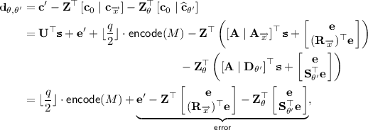
  where ${\mathbf {R}}_{{\overrightarrow{x}}}=\sum \limits _{i=1}^{\ell }\left( {\mathbf {R}}_i\mathbf {G}^{-1}(x_i\cdot \mathbf {G})\right)$. As in [1, 2, 13, 50], the above error term can be showed to be bounded by $s\ell m^{2}B\cdot \omega (\log n)=\widetilde{O}(\ell ^2 n^{3})$, with all but negligible probability. In order for the decryption algorithm to recover $\mathsf {encode}(M)$, and subsequently the plaintext M, it is required that the error term is bounded by q/5, i.e., $||\mathsf {error}||_{\infty }<q/5$. This is guaranteed by our setting of modulus q, i.e., $q= \widetilde{O}\left( \ell ^2 n^4 \right)$.

• 2. Suppose that $\langle {\overrightarrow{x}},{\overrightarrow{y}}\rangle \ne 0$. In this case, we have: ${\mathbf {c}}_{{\overrightarrow{x}}}=\big ({\mathbf {A}}_{{\overrightarrow{x}}}+\langle {\overrightarrow{x}},{\overrightarrow{y}}\rangle \cdot \mathbf {G}\big )^ \top {\mathbf {s}}+\sum \limits _{i=1}^{\ell }\left( {\mathbf {R}}_i\mathbf {G}^{-1}(x_i\cdot \mathbf {G}) \right) ^{\top }{{\mathbf {e}}}$. Then for each pair $(\theta ,\theta ')$, the following holds:

  

  Observe that the above contains the term ${\mathbf {Z}}^\top [{\mathbf {0}}\mid \langle {\overrightarrow{x}},{\overrightarrow{y}}\rangle \cdot \mathbf {G}]^\top {\mathbf {s}}$ which can be written as $\langle {\overrightarrow{x}},{\overrightarrow{y}}\rangle \cdot (\mathbf {G}{\mathbf {Z}}_2)^\top {\mathbf {s}}\in {\mathbb {Z}}_q^k$, where ${\mathbf {Z}}_2\in {\mathbb {Z}}^{m\times k}$ is the bottom part of matrix ${\mathbf {Z}}$. By Lemma 4, we have that the distribution of $\mathbf {G}{\mathbf {Z}}_2 \in \mathbb {Z}_q^{n \times k}$ is statistically close to uniform. This implies that, vector ${\mathbf {d}}_{\theta ,\theta '} \in \mathbb {Z}_q^k$, for each pair $(\theta ,\theta ')$, is indistinguishable from uniform. As a result, the probability that the last $k-1$ coordinates of vector $\lfloor \frac{2}{q} \cdot {\mathbf {d}}_{\theta ,\theta '} \rceil$ are all 0 is at most $2^{-(k-1)}=2^{-\omega (\log \lambda )}$, which is negligible in $\lambda$. In other words, except for negligible probability, the decryption algorithm outputs $\bot$ since it does not obtain a proper encoding $\mathsf {encode}(M) \in \{0,1\}^k$, for $M \in \{0,1\}$.

Efficiency. The efficiency aspect of our RPE scheme is as follows:

• The bit-size of public parameters $\textsf {pp}$ is $((\ell +2N)nm+nk)\log q=\big (\widetilde{O}(\ell ) + O(N)\big )\cdot \widetilde{O}\left( \lambda ^2 \right)$.

• The private key $\textsf {sk}_{{\overrightarrow{x}},I}$ has bit-size $O(\log N)\cdot \widetilde{O}\left( \lambda \right)$.

• The bit-size of ciphertext $\textsf {ct}$ is $\big (\widetilde{O}(\ell )+ O(r\log \frac{N}{r})\big )\cdot \widetilde{O}\left( \lambda \right)$.

The efficiency of our scheme is comparable to that of the pairing-based RPE scheme from [30, 31], in the following sense: the size of public parameters is O(N); the size of the private key is $O(\log N)$, and the ciphertext has size $O\left( r\log \frac{N}{r}\right)$ which is ranged between O(1) (when no key is revoked) and $O\left( \frac{N}{2}\right)$ (in the worst case when every second key is revoked).

In Sect. 4, we will discuss a variant of our scheme in the random oracle model, which has shorter public parameters.

Potential Implementation. While the focus of this work is to provide the first provably secure construction of RPE from lattice assumptions, it would be desirable to back it up with practical implementations and to compare the implementation details with those of pairing-based counterparts. However, this would be a highly challenging task, due to two main reasons:

• 1. We are not aware of any concrete implementation of the two building blocks of our scheme, i.e., the AFV PE [2, 50] and Agrawal et al.’s IBE [1].

• 2. In [30, 31], Nieto, Manulis and Sun did not provide implementation details of their pairing-based RPE scheme.

Given these circumstances, we leave the implementation aspect of our scheme as a future investigation. Nevertheless, in the following, we will discuss the potential of such implementation, by analyzing the main cryptographic operations needed for implementing the scheme. Apart from simple operations such as samplings of uniformly random matrices and vectors whose entries are in $\mathbb {Z}_q$ or $\{-1,1\}$, as well as multiplication and addition operations over $\mathbb {Z}_q$, the algorithms of the scheme requires the following time-consuming tasks:

• $\diamond$ Generation of a lattice trapdoor;

• $\diamond$ Samplings of discrete Gaussian vectors over lattices;

• $\diamond$ Samplings of LWE noise vectors.

We note that it is feasible to implement the listed above cryptographic tasks using the algorithms provided in [15, 26], which were recently improved in [14, 27]. Some implementation results of those cryptographic tasks were reported in [18], which may serve as a stepping stone of potential implementation of our scheme.

3.3 Security

In the following theorem, we prove that our scheme in Sect. 3 is selectively full hiding in the standard model, under the LWE assumption.

Theorem 1

Our RPE scheme satisfies the selective full-hiding security defined in Definition 3, assuming hardness of the $\left( {n,q,\chi }\right)$-$\mathsf {LWE}$ problem.

Proof

We proceed via a series of games, similar to those in [2, 13, 16]. First, we define the auxiliary algorithms for generating simulated public parameters, private keys and ciphertexts, and then, we describe the games.

Auxiliary algorithms. We consider the following auxiliary algorithms.

• $\mathsf {Sim.Setup}$ $\left( 1^{\lambda },{\mathbf {A}},{\mathbf {U}},{\overrightarrow{y}}^*,\textsf {RL}^*\right)$: On input a security parameter $\lambda$, a matrix ${\mathbf {A}}\in {\mathbb {Z}}_q^{n\times m}$, ${\mathbf {U}}\in {\mathbb {Z}}_q^{n\times k}$, the challenge attribute vector ${\overrightarrow{y}}^*=(y^*_1,\ldots ,y^*_\ell )\in {\mathbb {Z}}_q^{\ell }$ and revocation list $\textsf {RL}^*\subseteq [N]$, this algorithm performs the following steps:

  • 1. For each ${i\in [\ell ]}$, choose ${\mathbf {R}}_{i}\xleftarrow {\$}\{-1,1\}^{m\times m}$ and set ${\mathbf {A}}_{i}={\mathbf {A}}{\mathbf {R}}_{i}-y^*_i\cdot \mathbf {G}$.

  • 2. Build a binary tree $\mathsf {BT}$ and choose ${\mathbf {S}}_{\theta }\xleftarrow {\$}\{-1,1\}^{m\times m}$ for each ${\theta \in \mathsf {BT}}$. Set the identifier: ${\mathbf {D}}_{\theta }=\left\{ \begin{array}{ll} {\mathbf {A}}{\mathbf {S}}_{\theta }, &{} \text {if } \theta \in \mathsf {KUNodes}(\mathsf {BT},\textsf {RL}^*),\\ {\mathbf {A}}{\mathbf {S}}_{\theta }+\mathbf {G}, &{} \text {otherwise}. \end{array} \right.$

  • 3. Initialize the state $\textsf {ST}$.

  • 4. Output $\textsf {ST},\textsf {pp}=\left( {\mathbf {A}},\{{\mathbf {A}}_i\}_{i\in [\ell ]},{\mathbf {U}},\mathsf {BT}\right)$ and $\mathsf {msk}^*=(\{{\mathbf {R}}_i\}_{i\in [\ell ]},\{{\mathbf {S}}_{\theta }\}_{\theta \in \mathsf {BT}})$.

• $\mathsf {Sim.KeyGen}$ $\left( \mathsf {msk}^*,\textsf {ST},{\overrightarrow{x}},I,{\overrightarrow{y}}^*,\textsf {RL}^*\right)$: This algorithm takes as input $\mathsf {msk}^*$, state $\textsf {ST}$, a predicate vector ${\overrightarrow{x}}\in {\mathbb {Z}}_q^{\ell }$, an index $I\in [N]$, the challenge attribute vector ${\overrightarrow{y}}^*\in {\mathbb {Z}}_q^{\ell }$ and revocation list $\textsf {RL}^*\subseteq [N]$, such that the following condition holds: If $\langle {\overrightarrow{x}},{\overrightarrow{y}}^* \rangle = 0$ then $I\in \textsf {RL}^*$. The algorithm returns $\bot$ if $I\in \textsf {ST}$. Otherwise, it outputs the updated state $\textsf {ST}\leftarrow \textsf {ST}\cup \{I\}$ and private key $\textsf {sk}_{{\overrightarrow{x}},I}=\left( I,{\mathbf {Z}},\{{\mathbf {Z}}_{\theta }\}_{\theta \in \textsf {Path}({I})}\right)$ computed based on $\langle {\overrightarrow{x}},{\overrightarrow{y}}^* \rangle$ as follows.

  • 1. Case 1: $\langle {\overrightarrow{x}},{\overrightarrow{y}}^* \rangle \ne 0$.

    • (a) If $I\not \in \textsf {RL}^*$, then there is exactly one node $\theta ^*$ in the intersection $\textsf {Path}(I)\cap \mathsf {KUNodes}(\mathsf {BT},\textsf {RL}^*)$.

      Using Lemma 3, sample ${\mathbf {Z}}_{\theta ^*}\hookleftarrow \left( \mathcal {D}_{{\mathbb {Z}}^{2m},s}\right) ^k$ and set ${\mathbf {U}}_I={\mathbf {U}}-[{\mathbf {A}}\mid {\mathbf {D}}_{\theta ^*}]\cdot {\mathbf {Z}}_{\theta ^*}$. For each node $\theta \in \textsf {Path}(I)\backslash \{\theta ^*\}$, sample ${\mathbf {Z}}_{\theta }\leftarrow \mathsf {SampleRight}({\mathbf {A}},{\mathbf {S}}_{\theta },1,\mathbf {G},{\mathbf {T}}_{\mathbf {G}},{\mathbf {U}}-{\mathbf {U}}_{I},s)$. (See Sect. 2.1 for the description of algorithm SampleRight.)

    • (b) If $I\in \textsf {RL}^*$, choose ${\mathbf {U}}_I\xleftarrow {\$}{\mathbb {Z}}_q^{n\times k}$. Then for each $\theta \in \textsf {Path}(I)$, sample ${\mathbf {Z}}_{\theta }\leftarrow \mathsf {SampleRight}({\mathbf {A}},{\mathbf {S}}_{\theta },1,\mathbf {G},{\mathbf {T}}_{\mathbf {G}},{\mathbf {U}}-{\mathbf {U}}_{I},s).$

    As ${\mathbf {A}}_{{\overrightarrow{x}}}=\sum \limits _{i=1}^{\ell }{\mathbf {A}}_i\mathbf {G}^{-1} (x_i\cdot \mathbf {G}) ={\mathbf {A}}\big (\sum \limits _{i=1}^{\ell }{\mathbf {R}}_i\mathbf {G}^{-1}(x_i\cdot \mathbf {G})\big )-\underbrace{\langle {\overrightarrow{x}},{\overrightarrow{y}}^*\rangle }_{\ne 0}\cdot \mathbf {G}$, sample ${\mathbf {Z}}\leftarrow \mathsf {SampleRight}({\mathbf {A}},\sum \limits _{i=1}^{\ell }{\mathbf {R}}_i\mathbf {G}^{-1}(x_i\cdot \mathbf {G}),-\langle {\overrightarrow{x}},{\overrightarrow{y}}^* \rangle ,\mathbf {G},{\mathbf {T}}_{\mathbf {G}},{\mathbf {U}}_{I},s)$ satisfying $[{\mathbf {A}}\mid {\mathbf {A}}_{{\overrightarrow{x}}}]\cdot {\mathbf {Z}}={\mathbf {U}}_I$.

  • 2. Case 2: $\langle {\overrightarrow{x}},{\overrightarrow{y}}^* \rangle = 0$. In this case, the condition $I\in \textsf {RL}^*$ implies that $\textsf {Path}(I)\cap \mathsf {KUNodes}(\mathsf {BT},\textsf {RL}^*)=\emptyset$. Note that, here we do not have a trapdoor for the matrix $[{\mathbf {A}}\mid {\mathbf {A}}_{{\overrightarrow{x}}}]$, but we can instead compute ${\mathbf {Z}}$ and $\{{\mathbf {Z}}_{\theta }\}_{\theta \in \textsf {Path}(I)}$ as follows. First, we sample ${\mathbf {Z}}\hookleftarrow \left( \mathcal {D}_{{\mathbb {Z}}^{2m},s}\right) ^k$ and set ${\mathbf {U}}_I=[{\mathbf {A}}\mid {\mathbf {A}}_{{\overrightarrow{x}}}]\cdot {\mathbf {Z}}$. Then, for each $\theta \in \textsf {Path}(I)$, we sample ${\mathbf {Z}}_{\theta }\leftarrow \mathsf {SampleRight}({\mathbf {A}},{\mathbf {S}}_{\theta },1,\mathbf {G},{\mathbf {T}}_{\mathbf {G}},{\mathbf {U}}-{\mathbf {U}}_{I},s).$

• $\mathsf {Sim.Enc}$ $\left( \mathsf {msk}^*,M,{\mathbf {d}}_0,{\mathbf {d}}'\right)$: On input $\mathsf {msk}^*$, a message $M\in \{0,1\}$, and ${\mathbf {d}}_0\in {\mathbb {Z}}_q^m$, ${\mathbf {d}}'\in {\mathbb {Z}}_q^k$, it outputs $\textsf {ct}=\left( {\mathbf {c}}',{\mathbf {c}}_0, \{{\mathbf {c}}_i\}_{i\in [\ell ]},\{{\mathbf {c}}_{\theta }\}_{\theta \in \textsf {KUNodes}(\mathsf {BT},\textsf {RL})}\right)$, where:

  

The series of games. Let ${\mathcal {A}}$ be the adversary in the selective full-hiding game of Definition 3. We consider the following series of games.

• $\mathrm {Game}_0^{(b)}$: This game is the real security game in Definition 3, where the chosen bit is $b \in \{0,1\}$.

• $\mathrm {Game}_1^{(b)}$: This game is the same as $\mathrm {Game}_0^{(b)}$, except that algorithms $\mathsf {Setup}(1^\lambda )$ and $\mathsf {Enc}({\overrightarrow{y}}^{(b)},\textsf {RL}^{(b)},M^{(b)})$ are replaced by $\mathsf {Sim.Setup}\big (1^{\lambda },{\mathbf {A}},{\mathbf {U}},{\overrightarrow{y}}^{(b)},\textsf {RL}^{(b)}\big )$ and $\mathsf {Sim.Enc}\big (\mathsf {msk}^*,M^{(b)},{\mathbf {A}}^\top {\mathbf {s}}+{\mathbf {e}},{\mathbf {U}}^\top {\mathbf {s}}+{\mathbf {e}}'\big ),$ respectively, where ${\mathbf {A}}\xleftarrow {\$}{\mathbb {Z}}_q^{n\times m}$, ${\mathbf {U}}\xleftarrow {\$}{\mathbb {Z}}_q^{n}$, ${\mathbf {s}}\xleftarrow {\$}{\mathbb {Z}}_q^{n}$, ${\mathbf {e}}\hookleftarrow \chi ^m$, and ${\mathbf {e}}'\hookleftarrow \chi ^k$.

• $\mathrm {Game}_2^{(b)}$: It is the same as $\mathrm {Game}_1^{(b)}$, except that $\mathsf {KeyGen}\left( \textsf {msk},\textsf {ST},{\overrightarrow{x}}, I\right)$ is replaced by algorithm $\mathsf {Sim.KeyGen}\big (\mathsf {msk}^*,\textsf {ST},{\overrightarrow{x}},I,{\overrightarrow{y}}^{(b)},\textsf {RL}^{(b)}\big )$.

• $\mathrm {Game}_3^{(b)}$: It is the same as $\mathrm {Game}_2^{(b)}$, except that $\mathsf {Sim.Enc}\big (\mathsf {msk}^*,M^{(b)},{\mathbf {d}}_0,{\mathbf {d}}'\big )$ takes as inputs ${\mathbf {d}}_0\xleftarrow {\$}{\mathbb {Z}}_q^{m}$ and ${\mathbf {d}}'\xleftarrow {\$}{\mathbb {Z}}_q^k$.

• Game$_4$: In this final game, we make the following changes:

  • $\mathsf {Sim.Setup}\big (1^{\lambda },{\mathbf {A}},{\mathbf {U}},{\overrightarrow{y}}^{(b)},\textsf {RL}^{(b)}\big )$ is replaced by $\mathsf {Setup}(1^\lambda )$.

  • $\mathsf {Sim.KeyGen}(\mathsf {msk}^*,\textsf {ST},{\overrightarrow{x}},I,{\overrightarrow{y}}^{(b)},\textsf {RL}^{(b)})$ is replaced by $\mathsf {KeyGen}\big (\textsf {msk},\textsf {ST},{\overrightarrow{x}},I\big )$.

  • Instead of computing ${\mathbf {c}}' = {\mathbf {d}}'+\lfloor \frac{q}{2} \rfloor \cdot \mathsf {encode}(M^{(b)})\in {\mathbb {Z}}_q^k$, we sample ${\mathbf {c}}' \xleftarrow {\$} {\mathbb {Z}}_q^k$.

To prove Theorem 1, we will first demonstrate in the following lemmas that any two consecutive games in the above series are either statistically indistinguishable or computationally indistinguishable under the LWE assumption.

Lemma 6

${\mathcal {A}}$’s view in $\mathrm {Game}_0^{(b)}$ is statistically close to the view in $\mathrm {Game}_1^{(b)}$.

Proof

We will show that the public parameters $\textsf {pp}=\left( {\mathbf {A}},\{{\mathbf {A}}_i\}_{i\in [\ell ]},{\mathbf {U}},\mathsf {BT}\right)$ and ciphertext $\textsf {ct}=\big ({\mathbf {c}}',{\mathbf {c}}_0, \{{\mathbf {c}}_i\}_{i\in [\ell ]},\{\widehat{{\mathbf {c}}}_{\theta }\}_{\theta \in \textsf {KUNodes}(\mathsf {BT},\textsf {RL})}\big )$ produced by algorithms $\mathsf {Sim.Setup}\big (1^{\lambda },{\mathbf {A}},{\mathbf {U}},{\overrightarrow{y}}^{(b)},\textsf {RL}^{(b)}\big )$ and $\mathsf {Sim.Enc}(\mathsf {msk}^*,M^{(b)},{\mathbf {A}}^\top {\mathbf {s}}+{\mathbf {e}},{\mathbf {U}}^\top {\mathbf {s}}+{\mathbf {e}}')$ in $\mathrm {Game}_1^{(b)}$ are statistically close to those by $\mathsf {Setup}$ and $\mathsf {Enc}$ respectively, in $\mathrm {Game}_0^{(b)}$.

Firstly, we observe that matrix ${\mathbf {A}}$ is truly uniform in $\mathrm {Game}_1^{(b)}$. In $\mathrm {Game}_0^{(b)}$, it is generated via algorithm $\textsf {TrapGen}$, and is statistically close to uniform over ${\mathbb {Z}}_q^{n\times m}$ by Lemma 1. Furthermore, ${\mathbf {U}}\in \mathbb {Z}_q^{n \times k}$ is truly uniform in both games.

Let ${\overrightarrow{y}}^{(b)} = (y^{(b)}_1, \ldots , y^{(b)}_\ell )$. For each $i\in [\ell ]$ and each $\theta \in \mathsf {BT}$, the matrices ${\mathbf {A}}_i,{\mathbf {D}}_{\theta }\in {\mathbb {Z}}_q^{n\times m}$ are truly uniform in $\mathrm {Game}_0^{(b)}$, while in $\mathrm {Game}_1^{(b)}$, they are set as ${\mathbf {A}}_i={\mathbf {A}}{\mathbf {R}}_{i}-y^{(b)}_i\cdot \mathbf {G}, {\mathbf {D}}_{\theta }={\mathbf {A}}{\mathbf {S}}_{\theta }+ \rho _\theta \cdot \mathbf {G},$ where ${\mathbf {R}}_i, {\mathbf {S}}_\theta \xleftarrow {\$} \{-1,1\}^{m \times m}$ and $\rho _{\theta } \in \{0,1\}$. Then, the ciphertext components ${\mathbf {c}}'$, ${\mathbf {c}}_0$, $\{{\mathbf {c}}_i\}_{i\in [\ell ]}$ and $\{\widehat{{\mathbf {c}}}_{\theta }\}_{\theta \in \textsf {KUNodes}(\mathsf {BT},\textsf {RL})}$ in both games can be expressed as:

where ${\mathbf {s}}\xleftarrow {\$}{\mathbb {Z}}_q^n$, ${\mathbf {e}}'\hookleftarrow \chi ^k$ and ${\mathbf {e}}\hookleftarrow \chi ^m$. By Lemma 5, the joint distributions of $\left( {\mathbf {A}}, {\mathbf {A}}{\mathbf {R}}_i-{\overrightarrow{y}}^{(b)}_i\cdot \mathbf {G}, {\mathbf {R}}_i^\top {\mathbf {e}}\right) \text { and } \left( {\mathbf {A}},{\mathbf {A}}_i,{\mathbf {R}}_i^\top {\mathbf {e}}\right) ,$ $\left( {\mathbf {A}}, {\mathbf {A}}{\mathbf {S}}_\theta + \rho _\theta \cdot \mathbf {G}, {\mathbf {S}}_\theta ^\top {\mathbf {e}}\right)$ and $\left( {\mathbf {A}},{\mathbf {D}}_\theta ,{\mathbf {S}}_\theta ^\top {\mathbf {e}}\right)$ as statistically indistinguishable. It implies that the distributions of $\big ({\mathbf {A}},\{{\mathbf {A}}_i\}_{i\in [\ell ]}, {\mathbf {U}}, \{{\mathbf {D}}_\theta \}_{\theta \in \mathsf {BT}}, {\mathbf {c}}', {\mathbf {c}}_0, \{{\mathbf {c}}_i\}_{i\in [\ell ]}, \{\widehat{{\mathbf {c}}}_{\theta }\}_{\theta \in \textsf {KUNodes}(\mathsf {BT},\textsf {RL})} \big )$ in $\mathrm {Game}_0^{(b)}$ and $\mathrm {Game}_1^{(b)}$ are statistically indistinguishable. This concludes the lemma.    $\square$

Lemma 7

${\mathcal {A}}$’s view in $\mathrm {Game}_1^{(b)}$ is statistically close to the view in $\mathrm {Game}_2^{(b)}$.

Proof

Recall that, from $\mathrm {Game}_1^{(b)}$ to $\mathrm {Game}_2^{(b)}$, we replace the real key generation algorithm $\mathsf {KeyGen}$ by $\mathsf {Sim.KeyGen}$. Thus, we need to show that for all queries of the form $({\overrightarrow{x}},I)$ from ${\mathcal {A}}$, the private keys $\textsf {sk}_{{\overrightarrow{x}},I}=\left( I,{\mathbf {Z}},\{{\mathbf {Z}}_{\theta }\}_{\theta \in \textsf {Path}({I})}\right)$ outputted by $\mathsf {Sim.KeyGen}$ and $\mathsf {KeyGen}$ are statistically indistinguishable.

We first note that, in both cases, matrices ${\mathbf {Z}}\in \mathbb {Z}^{2m \times k},\{{\mathbf {Z}}_{\theta } \in \mathbb {Z}^{2m \times k}\}_{\theta \in \textsf {Path}({I})}$ satisfy $[{\mathbf {A}}\mid {\mathbf {A}}_{{\overrightarrow{x}}}]\cdot {\mathbf {Z}}+ [{\mathbf {A}}\mid {\mathbf {D}}_{\theta }]\cdot {\mathbf {Z}}_{\theta } = \mathbf {U}, \forall \theta \in \textsf {Path}({I}).$ Next, we observe that, in $\mathsf {KeyGen}$, the columns of these matrices are sampled via algorithm $\mathsf {SampleLeft}$, while in $\mathsf {Sim.KeyGen}$, they are either sampled via algorithm $\mathsf {SampleRight}$ or sampled from $\mathcal {D}_{{\mathbb {Z}}^{m},s}$. The properties of these sampling algorithms (see Sect. 2) then guarantee that the two distributions are statistically indistinguishable.    $\square$

Lemma 8

Under the $(n,q,\chi )$-$\mathsf {LWE}$ assumption, ${\mathcal {A}}$’s view in $\mathrm {Game}_2^{(b)}$ is computationally indistinguishable from the view in $\mathrm {Game}_3^{(b)}$.

Proof

From $\mathrm {Game}_2^{(b)}$ to $\mathrm {Game}_3^{(b)}$, we change the inputs ${\mathbf {d}}_0,{\mathbf {d}}'$ to algorithm $\mathsf {Sim.Enc}$ from $\textsf {LWE}$ instances to uniformly random vectors in $\mathbb {Z}_q^m$ and $\mathbb {Z}_q^k$, respectively. Suppose that ${\mathcal {A}}$ has non-negligible advantage in distinguishing $\mathrm {Game}_2^{(b)}$ from $\mathrm {Game}_3^{(b)}$. We use ${\mathcal {A}}$ to construct an LWE solver ${\mathcal {B}}$ as follows:

• ${\mathcal {B}}$ requests for $m+k$ LWE instances $\{(\mathbf {a}_j,v_j)\in {\mathbb {Z}}_q^n\times {\mathbb {Z}}_q\}_{j \in [m+k]}$.

• ${\mathcal {B}}$ forms the following matrices and vectors: ${\mathbf {A}}=[\mathbf {a}_1,\ldots ,\mathbf {a}_m]\in {\mathbb {Z}}_q^{n\times m}$, ${\mathbf {U}}=[\mathbf {a}_{m+1},\ldots ,\mathbf {a}_{m+k}]\in {\mathbb {Z}}_q^{n\times k}$, ${\mathbf {d}}_0 =[v_1,\cdots ,v_m]^\top \in {\mathbb {Z}}_q^{ m}$, ${\mathbf {d}}'=[v_{m+1},\cdots ,v_{m+k}]^\top$ $\in {\mathbb {Z}}_q^{ k}$, and runs $\mathsf {Sim.Setup}\big (1^{\lambda },{\mathbf {A}},{\mathbf {U}},{\overrightarrow{y}}^{(b)},\textsf {RL}^{(b)}\big )$ as in $\mathrm {Game}_2^{(b)}$.

• ${\mathcal {B}}$ answers the private key queries of the form $({\overrightarrow{x}},I)$, as in $\mathrm {Game}_2^{(b)}$, by running algorithm $\mathsf {Sim.KeyGen}\big (\mathsf {msk}^*,\textsf {ST},{\overrightarrow{x}},I,{\overrightarrow{y}}^{(b)},\textsf {RL}^{(b)}\big )$.

• When receiving from ${\mathcal {A}}$ two messages $M^{(0)},M^{(1)}\in \{0,1\}$, ${\mathcal {B}}$ prepares a challenge ciphertext $\textsf {ct}^*$ by running $\mathsf {Sim.Enc}\left( \mathsf {msk}^*,M^{(b)},{\mathbf {d}}_0,{\mathbf {d}}'\right)$.

• Finally, after being allowed to make additional queries, ${\mathcal {A}}$ guesses whether it is interacting with $\mathrm {Game}_2^{(b)}$ or $\mathrm {Game}_3^{(b)}$. Then, ${\mathcal {B}}$ outputs ${\mathcal {A}}$’s guess as the answer to the $\textsf {LWE}$ challenger.

Recall that by Definition 1, for each $j\in [m+k]$, either $v_j=\langle \mathbf {a}_j,{\mathbf {s}}\rangle +e_j$ for secret ${\mathbf {s}}\xleftarrow {\$}{\mathbb {Z}}_q^n$ and noise $e_j\hookleftarrow \chi$; or $v_j$ is uniformly random in ${\mathbb {Z}}_q$. On the one hand, if $v_j=\langle \mathbf {a}_j,{\mathbf {s}}\rangle +e_j$, then the adversary ${\mathcal {A}}$’s view is as in $\mathrm {Game}_2^{(b)}$. On the other hand, if $v_j$ is uniformly random in ${\mathbb {Z}}_q$, then ${\mathcal {A}}$’s view is as in $\mathrm {Game}_2^{(b)}$. Hence, algorithm ${\mathcal {B}}$ can solve the $(n,q,\chi )$-$\mathsf {LWE}$ problem with non-negligible probability, assuming that the adversary ${\mathcal {A}}$ can distinguish $\mathrm {Game}_2^{(b)}$ from $\mathrm {Game}_3^{(b)}$ with non-negligible advantage. This concludes the lemma.    $\square$

Lemma 9

${\mathcal {A}}$’s view in $\mathrm {Game}_3^{(b)}$ is statistically close to the view in $\mathrm {Game}_4$.

Proof

Firstly, based on the same argument as in Lemma 6, we can deduce that the output of algorithm $\mathsf {Sim.Setup}\big (1^{\lambda },{\mathbf {A}},{\mathbf {U}},{\overrightarrow{y}}^{(b)},\textsf {RL}^{(b)}\big )$ in $\mathrm {Game}_3^{(b)}$ is statistically close that of $\mathsf {Setup}(1^\lambda )$ in $\mathrm {Game}_4$.

Secondly, based on the same argument as in Lemma 7, we can deduce that the output of algorithm $\mathsf {Sim.KeyGen}\big (\mathsf {msk}^*,\textsf {ST},{\overrightarrow{x}},I,{\overrightarrow{y}}^{(b)},\textsf {RL}^{(b)}\big )$ in $\mathrm {Game}_3^{(b)}$ is statistically close to that of $\mathsf {KeyGen}\big (\textsf {msk},\textsf {ST},{\overrightarrow{x}}, I\big )$ in $\mathrm {Game}_4$.

Finally, the shift from ${\mathbf {c}}' = {\mathbf {d}}'+\lfloor \frac{q}{2} \rfloor \cdot \mathsf {encode}(M^{(b)})\in {\mathbb {Z}}_q^k$ to a uniformly random ${\mathbf {c}}' \in {\mathbb {Z}}_q^k$ is only a conceptual change, because vector ${\mathbf {d}}'$ in $\mathrm {Game}_3^{(b)}$ is uniformly random over ${\mathbb {Z}}_q^k$.    $\square$

The theorem now follows from the fact that the advantage of ${\mathcal {A}}$ in Game$_4$ is 0, since Game$_4$ no longer depends on the bit b.    $\square$

4 Extensions and Open Questions

In this section, we discuss several possible extensions of our lattice-based RPE scheme, as well as some questions that we left open.

4.1 Extensions

Multi-bit version. The scheme presented in Sect. 3 only allows to encrypt 1-bit messages. Using standard techniques for multi-bit LWE-based encryption, e.g., [1, 15, 37], we can achieve a $\tau$-bit variant with small overhead, for any $\tau = \mathsf {poly}(\lambda )$. A notable change in this case is that we will employ a revised encoding function $\mathsf {encode}': \{0,1\}^\tau \rightarrow \{0,1\}^{\tau + k}$, where for any $\mu \in \{0,1\}^\tau$, vector $\mathsf {encode}'(\mu )$ is obtained by appending $k = \omega (\log \lambda )$ entries 0 to vector $\mu$.

Better efficiency in the random oracle model. The RPE scheme from Sect. 3 has relatively large public parameters $\textsf {pp}$, i.e., of bit-size $\big (\widetilde{O}(\ell ) + O(N)\big )\cdot \widetilde{O}(\lambda ^2)$, for which the dependence on N is due to the fact that we have to associate each node $\theta$ in the binary tree with a uniformly random matrix in $\mathbf {D}_\theta \in {\mathbb {Z}}_q^{n\times m}$, in order to obtain full-hiding security in the standard model. Fortunately, the size of $\textsf {pp}$ can be reduced to $\widetilde{O}(\ell )\cdot \widetilde{O}(\lambda ^2)$ (which is comparable to that of the underlying PE scheme [2, 50]), if we work in the random oracle model [7]. The idea is as follows.

Let $\mathcal {H}: \{0,1\}^* \rightarrow {\mathbb {Z}}_q^{n\times m}$ be a random oracle. Then, in the scheme, for each node $\theta$, we obtain uniformly random matrix $\mathbf {D}_\theta$ as $\mathbf {D}_\theta : = \mathcal {H}({\mathbf {A}},\{{\mathbf {A}}_i\}_{i\in [\ell ]},{\mathbf {U}}, \theta )$. The rest of the scheme remains the same. In the security proof, we first simulate the generation of $\mathbf {D}_\theta$ as in the proof of Theorem 1. Then, it remains to program the random oracle such that $\mathcal {H}({\mathbf {A}},\{{\mathbf {A}}_i\}_{i\in [\ell ]},{\mathbf {U}}, \theta ): = \mathbf {D}_\theta$. This modification allows us to make the size of $\textsf {pp}$ independent of N.

4.2 Open Questions

We introduced the first revocable predicate encryption scheme based on the LWE assumption. While the pairing-based scheme from [30, 31] achieved adaptive full-hiding security, our construction is only proven secure in the selective setting. Achieving the stronger notion of [30, 31] seems to require that the underlying PE be adaptively secure. However, to the best of our knowledge, existing lattice-based PE schemes [2, 13, 16, 50] only achieved selective security. We therefore view the problem of constructing adaptively secure lattice-based RPE as an interesting open question.

Finally, as shown in [19, 50], some applications of PE for inner-product predicate over $R^\ell$ (in our scheme, $R = \mathbb {Z}_q$) require that R has exponentially large cardinality. Those include implementations of PE for CNF formulae [19] and hidden vector encryption [10]. However, for our scheme, this requires to set the modulus q to be exponential in $\lambda$. Hence, it would be desirable to achieve a lattice-based PE scheme supporting both revocation and exponentially large R, that demands only polynomial moduli. One possible approach towards tackling this question is to adapt the techniques introduced by Xagawa [50], where one works with $R = \mathrm {GF}(q^n)$ instead of $\mathbb {Z}_q$.

References

Agrawal, S., Boneh, D., Boyen, X.: Efficient lattice (H)IBE in the standard model. In: Gilbert, H. (ed.) EUROCRYPT 2010. LNCS, vol. 6110, pp. 553–572. Springer, Heidelberg (2010). doi:10.1007/978-3-642-13190-5_28
Agrawal, S., Freeman, D.M., Vaikuntanathan, V.: Functional encryption for inner product predicates from learning with errors. In: Lee, D.H., Wang, X. (eds.) ASIACRYPT 2011. LNCS, vol. 7073, pp. 21–40. Springer, Heidelberg (2011). doi:10.1007/978-3-642-25385-0_2
Ajtai, M.: Generating hard instances of the short basis problem. In: Wiedermann, J., van Emde Boas, P., Nielsen, M. (eds.) ICALP 1999. LNCS, vol. 1644, pp. 1–9. Springer, Heidelberg (1999). doi:10.1007/3-540-48523-6_1
Alwen, J., Peikert, C.: Generating shorter bases for hard random lattices. Theory Comput. Syst. 48(3), 535–553 (2011)
Attrapadung, N., Imai, H.: Attribute-based encryption supporting direct/indirect revocation modes. In: Parker, M.G. (ed.) IMACC 2009. LNCS, vol. 5921, pp. 278–300. Springer, Heidelberg (2009). doi:10.1007/978-3-642-10868-6_17
Attrapadung, N., Libert, B.: Functional encryption for inner product: achieving constant-size ciphertexts with adaptive security or support for negation. In: Nguyen, P.Q., Pointcheval, D. (eds.) PKC 2010. LNCS, vol. 6056, pp. 384–402. Springer, Heidelberg (2010). doi:10.1007/978-3-642-13013-7_23
Bellare, M., Rogaway, P.: Random oracles are practical: a paradigm for designing efficient protocols. In: CCS 1993, pp. 62–73. ACM (1993)
Boldyreva, A., Goyal, V., Kumar, V.: Identity-based encryption with efficient revocation. In: CCS 2008, pp. 417–426. ACM (2008)
Boneh, D., Franklin, M.: Identity-based encryption from the weil pairing. In: Kilian, J. (ed.) CRYPTO 2001. LNCS, vol. 2139, pp. 213–229. Springer, Heidelberg (2001). doi:10.1007/3-540-44647-8_13
Boneh, D., Waters, B.: Conjunctive, subset, and range queries on encrypted data. In: Vadhan, S.P. (ed.) TCC 2007. LNCS, vol. 4392, pp. 535–554. Springer, Heidelberg (2007). doi:10.1007/978-3-540-70936-7_29
Chen, J., Lim, H.W., Ling, S., Wang, H., Nguyen, K.: Revocable identity-based encryption from lattices. In: Susilo, W., Mu, Y., Seberry, J. (eds.) ACISP 2012. LNCS, vol. 7372, pp. 390–403. Springer, Heidelberg (2012). doi:10.1007/978-3-642-31448-3_29
Cheng, S., Zhang, J.: Adaptive-ID secure revocable identity-based encryption from lattices via subset difference method. In: Lopez, J., Wu, Y. (eds.) ISPEC 2015. LNCS, vol. 9065, pp. 283–297. Springer, Cham (2015). doi:10.1007/978-3-319-17533-1_20
Gay, R., Méaux, P., Wee, H.: Predicate encryption for multi-dimensional range queries from lattices. In: Katz, J. (ed.) PKC 2015. LNCS, vol. 9020, pp. 752–776. Springer, Heidelberg (2015). doi:10.1007/978-3-662-46447-2_34
Genise, N., Micciancio, D.: Faster gaussian sampling for trapdoor lattices with arbitrary modulus. IACR Cryptology ePrint Archive 2017:308 (2017)
Gentry, C., Peikert, C., Vaikuntanathan, V.: Trapdoors for hard lattices and new cryptographic constructions. In: STOC 2008, pp. 197–206. ACM (2008)
Gorbunov, S., Vaikuntanathan, V., Wee, H.: Predicate encryption for circuits from LWE. In: Gennaro, R., Robshaw, M. (eds.) CRYPTO 2015. LNCS, vol. 9216, pp. 503–523. Springer, Heidelberg (2015). doi:10.1007/978-3-662-48000-7_25
Goyal, V., Pandey, O., Sahai, A., Waters, B.: Attribute-based encryption for fine-grained access control of encrypted data. In: CCS 2006, pp. 89–98. ACM (2006)
Gur, K.D., Polyakov, Y., Rohloff, K., Ryan, G.W., Savas, E.: Implementation and evaluation of improved Gaussian sampling for lattice trapdoors. IACR Cryptology ePrint Archive, 2017:285 (2017)
Katz, J., Sahai, A., Waters, B.: Predicate encryption supporting disjunctions, polynomial equations, and inner products. In: Smart, N. (ed.) EUROCRYPT 2008. LNCS, vol. 4965, pp. 146–162. Springer, Heidelberg (2008). doi:10.1007/978-3-540-78967-3_9
Lee, K., Kim, I., Hwang, S.O.: Privacy preserving revocable predicate encryption revisited. Secur. Commun. Netw. 8(3), 471–485 (2015)
Lewko, A., Okamoto, T., Sahai, A., Takashima, K., Waters, B.: Fully secure functional encryption: attribute-based encryption and (hierarchical) inner product encryption. In: Gilbert, H. (ed.) EUROCRYPT 2010. LNCS, vol. 6110, pp. 62–91. Springer, Heidelberg (2010). doi:10.1007/978-3-642-13190-5_4
Libert, B., Peters, T., Yung, M.: Group signatures with almost-for-free revocation. In: Safavi-Naini, R., Canetti, R. (eds.) CRYPTO 2012. LNCS, vol. 7417, pp. 571–589. Springer, Heidelberg (2012). doi:10.1007/978-3-642-32009-5_34
Libert, B., Peters, T., Yung, M.: Scalable group signatures with revocation. In: Pointcheval, D., Johansson, T. (eds.) EUROCRYPT 2012. LNCS, vol. 7237, pp. 609–627. Springer, Heidelberg (2012). doi:10.1007/978-3-642-29011-4_36
Libert, B., Vergnaud, D.: Adaptive-ID secure revocable identity-based encryption. In: Fischlin, M. (ed.) CT-RSA 2009. LNCS, vol. 5473, pp. 1–15. Springer, Heidelberg (2009). doi:10.1007/978-3-642-00862-7_1
Micciancio, D., Mol, P.: Pseudorandom knapsacks and the sample complexity of lwe search-to-decision reductions. In: Rogaway, P. (ed.) CRYPTO 2011. LNCS, vol. 6841, pp. 465–484. Springer, Heidelberg (2011). doi:10.1007/978-3-642-22792-9_26
Micciancio, D., Peikert, C.: Trapdoors for lattices: simpler, tighter, faster, smaller. In: Pointcheval, D., Johansson, T. (eds.) EUROCRYPT 2012. LNCS, vol. 7237, pp. 700–718. Springer, Heidelberg (2012). doi:10.1007/978-3-642-29011-4_41
Micciancio, D., Walter, M.: Gaussian sampling over the integers: efficient, generic, constant-time. IACR Cryptology ePrint Archive 2017:259 (2017)
Naor, D., Naor, M., Lotspiech, J.: Revocation and tracing schemes for stateless receivers. In: Kilian, J. (ed.) CRYPTO 2001. LNCS, vol. 2139, pp. 41–62. Springer, Heidelberg (2001). doi:10.1007/3-540-44647-8_3
Nguyen, K., Wang, H., Zhang, J.: Server-aided revocable identity-based encryption from lattices. In: Foresti, S., Persiano, G. (eds.) CANS 2016. LNCS, vol. 10052, pp. 107–123. Springer, Cham (2016). doi:10.1007/978-3-319-48965-0_7
González-Nieto, J.M., Manulis, M., Sun, D.: Fully private revocable predicate encryption. In: Susilo, W., Mu, Y., Seberry, J. (eds.) ACISP 2012. LNCS, vol. 7372, pp. 350–363. Springer, Heidelberg (2012). doi:10.1007/978-3-642-31448-3_26
Gonźalez-Nieto, J.M., Manulis, M., Sun, D.: Fully private revocable predicate encryption. IACR Cryptology ePrint Archive 2012:403 (2012)
Okamoto, T., Takashima, K.: Hierarchical predicate encryption for inner-products. In: Matsui, M. (ed.) ASIACRYPT 2009. LNCS, vol. 5912, pp. 214–231. Springer, Heidelberg (2009). doi:10.1007/978-3-642-10366-7_13
Okamoto, T., Takashima, K.: Fully secure functional encryption with general relations from the decisional linear assumption. In: Rabin, T. (ed.) CRYPTO 2010. LNCS, vol. 6223, pp. 191–208. Springer, Heidelberg (2010). doi:10.1007/978-3-642-14623-7_11
Okamoto, T., Takashima, K.: Achieving short ciphertexts or short secret-keys for adaptively secure general inner-product encryption. In: Lin, D., Tsudik, G., Wang, X. (eds.) CANS 2011. LNCS, vol. 7092, pp. 138–159. Springer, Heidelberg (2011). doi:10.1007/978-3-642-25513-7_11
Okamoto, T., Takashima, K.: Adaptively attribute-hiding (hierarchical) inner product encryption. In: Pointcheval, D., Johansson, T. (eds.) EUROCRYPT 2012. LNCS, vol. 7237, pp. 591–608. Springer, Heidelberg (2012). doi:10.1007/978-3-642-29011-4_35
Peikert, C.: Public-key cryptosystems from the worst-case shortest vector problem: extended abstract. In: STOC 2009, pp. 333–342. ACM (2009)
Peikert, C., Vaikuntanathan, V., Waters, B.: A framework for efficient and composable oblivious transfer. In: Wagner, D. (ed.) CRYPTO 2008. LNCS, vol. 5157, pp. 554–571. Springer, Heidelberg (2008). doi:10.1007/978-3-540-85174-5_31
Regev, O.: On lattices, learning with errors, random linear codes, and cryptography. In: STOC 2005, pp. 84–93. ACM (2005)
Sahai, A., Seyalioglu, H., Waters, B.: Dynamic credentials and ciphertext delegation for attribute-based encryption. In: Safavi-Naini, R., Canetti, R. (eds.) CRYPTO 2012. LNCS, vol. 7417, pp. 199–217. Springer, Heidelberg (2012). doi:10.1007/978-3-642-32009-5_13
Sahai, A., Waters, B.: Fuzzy identity-based encryption. In: Cramer, R. (ed.) EUROCRYPT 2005. LNCS, vol. 3494, pp. 457–473. Springer, Heidelberg (2005). doi:10.1007/11426639_27
Seo, J.H., Emura, K.: Efficient delegation of key generation and revocation functionalities in identity-based encryption. In: Dawson, E. (ed.) CT-RSA 2013. LNCS, vol. 7779, pp. 343–358. Springer, Heidelberg (2013). doi:10.1007/978-3-642-36095-4_22
Seo, J.H., Emura, K.: Revocable identity-based encryption revisited: security model and construction. In: Kurosawa, K., Hanaoka, G. (eds.) PKC 2013. LNCS, vol. 7778, pp. 216–234. Springer, Heidelberg (2013). doi:10.1007/978-3-642-36362-7_14
Seo, J.H., Emura, K.: Revocable hierarchical identity-based encryption. Theor. Comput. Sci. 542, 44–62 (2014)
Seo, J.H., Emura, K.: Revocable identity-based cryptosystem revisited: security sodels and constructions. IEEE Trans. Inf. Forensics Secur. 9(7), 1193–1205 (2014)
Seo, J.H., Emura, K.: Adaptive-ID secure revocable hierarchical identity-based encryption. In: Tanaka, K., Suga, Y. (eds.) IWSEC 2015. LNCS, vol. 9241, pp. 21–38. Springer, Cham (2015). doi:10.1007/978-3-319-22425-1_2
Shi, E., Bethencourt, J., Chan, H.T.-H., Song, D.X., Perrig, A.: Multi-dimensional range query over encrypted data. In: IEEE Symposium on Security and Privacy (S&P 2007), pp. 350–364. IEEE Computer Society (2007)
Takayasu, A., Watanabe, Y.: Lattice-based revocable identity-based encryption with bounded decryption key exposure resistance. In: Pieprzyk, J., Suriadi, S. (eds.) ACISP 2017. LNCS, vol. 10342, pp. 184–204. Springer, Cham (2017). doi:10.1007/978-3-319-60055-0_10
Watanabe, Y., Emura, K., Seo, J.H.: New revocable IBE in prime-order groups: adaptively secure, decryption key exposure resistant, and with short public parameters. In: Handschuh, H. (ed.) CT-RSA 2017. LNCS, vol. 10159, pp. 432–449. Springer, Cham (2017). doi:10.1007/978-3-319-52153-4_25
Waters, B.: Dual system encryption: realizing fully secure IBE and HIBE under simple assumptions. In: Halevi, S. (ed.) CRYPTO 2009. LNCS, vol. 5677, pp. 619–636. Springer, Heidelberg (2009). doi:10.1007/978-3-642-03356-8_36
Xagawa, K.: Improved (hierarchical) inner-product encryption from lattices. In: Kurosawa, K., Hanaoka, G. (eds.) PKC 2013. LNCS, vol. 7778, pp. 235–252. Springer, Heidelberg (2013). doi:10.1007/978-3-642-36362-7_15
Acknowledgements
We thank the reviewers for helpful discussions and comments. The research was supported by the “Singapore Ministry of Education under Research Grant MOE2016-T2-2-014(S)”. Huaxiong Wang was also supported by NTU under Tier 1 grant RG143/14.
Author information
Authors and Affiliations
Corresponding author
Editor information
Editors and Affiliations
Rights and permissions
Copyright information
© 2017 Springer International Publishing AG
About this paper
Cite this paper
Ling, S., Nguyen, K., Wang, H., Zhang, J. (2017). Revocable Predicate Encryption from Lattices. In: Okamoto, T., Yu, Y., Au, M., Li, Y. (eds) Provable Security. ProvSec 2017. Lecture Notes in Computer Science(), vol 10592. Springer, Cham. https://doi.org/10.1007/978-3-319-68637-0_19
Download citation
DOI: https://doi.org/10.1007/978-3-319-68637-0_19
Published:
Publisher Name: Springer, Cham
Print ISBN: 978-3-319-68636-3
Online ISBN: 978-3-319-68637-0
eBook Packages: Computer ScienceComputer Science (R0)