Appendix A: Background on Differentiable Manifolds

Abstract

From a mathematical point of view, gauge theories are described by a spacetime M together with certain fibre bundles (principal bundles, associated vector bundles, spinor bundles) over M. Spacetime and fibre bundles are assumed to have the structure of differentiable manifolds. Differentiable manifolds in turn are certain topological spaces that essentially have the property of being locally Euclidean, i.e. locally look like an open set in some $\mathbb{R}^{n}$, and that have a differentiable structure, so that we can define differentiable maps (and their derivatives), vector fields, differential forms, etc. on them.

From a mathematical point of view, gauge theories are described by a spacetime M together with certain fibre bundles (principal bundles, associated vector bundles, spinor bundles) over M. Spacetime and fibre bundles are assumed to have the structure of differentiable manifolds. Differentiable manifolds in turn are certain topological spaces that essentially have the property of being locally Euclidean, i.e. locally look like an open set in some $\mathbb{R}^{n}$, and that have a differentiable structure, so that we can define differentiable maps (and their derivatives), vector fields, differential forms, etc. on them.

We briefly sketch the definitions of these concepts. More details can be found in any textbook on differentiable manifolds or differential geometry, like [84] and [142].

A.1 Manifolds

A.1.1 Topological Manifolds

Topological manifolds are topological spaces with certain additional structures. They are a first step towards differentiable manifolds, which are the main spaces that we will consider in this book.

Definition A.1.1

An n -dimensional topological manifold , also called a topological n -manifold, is a topological space M such that:

• 1. M is locally Euclidean , i.e. locally homeomorphic to $\mathbb{R}^{n}$. This means that around every point p ∈ M there exists an open neighbourhood U ⊂ M that is homeomorphic to some open set $V \subset \mathbb{R}^{n}$ (both open sets with the subspace topology).

• 2. M is Hausdorff.

• 3. M has a countable basis for its topology.

The local homeomorphisms $\phi: M \supset U \rightarrow V \subset \mathbb{R}^{n}$ (and sometimes the subsets U) are called charts or local coordinate systems for M. Axiom (a) says that we can cover the whole manifold M by charts. Note that the dimension n is assumed to be the same over the whole manifold. Axiom (c) is of a technical nature and usually can be neglected for our purposes. We often denote an n-manifold by M ⁿ.

Example A.1.2

The simplest topological n-manifold is $M = \mathbb{R}^{n}$ itself. We can cover M by one chart $\phi: \mathbb{R}^{n} \rightarrow \mathbb{R}^{n}$, given by the identity.

Example A.1.3

Another example of a topological n-manifold is the n -sphere M = S ⁿ for n ≥ 0. We define

$$\displaystyle{ S^{n} =\{ x \in \mathbb{R}^{n+1}\mid \vert \vert x\vert \vert = 1\}. }$$

Here | | x | | denotes the Euclidean norm. We endow S ⁿ with the subspace topology of $\mathbb{R}^{n+1}$. It follows that S ⁿ is Hausdorff, compact and has a countable basis for its topology.

We thus only have to cover S ⁿ by charts that define local homeomorphisms to $\mathbb{R}^{n}$. A very useful choice are two charts given by stereographic projection . We think of $\mathbb{R}^{n}$ as the hyperplane {x _n+1 = 0} in $\mathbb{R}^{n+1}$. We then project a point x in U _N = S ⁿ ∖{N}, where N is the north pole

$$\displaystyle{ N = (0,\ldots,0,+1) \in S^{n} \subset \mathbb{R}^{n+1}, }$$

along the line through N and x onto the hyperplane $\mathbb{R}^{n}$. It is easy to check that this defines a map

$$\displaystyle\begin{array}{rcl} \phi _{N}: U_{N}& \longrightarrow & \mathbb{R}^{n} {}\\ x& \longmapsto & \frac{1} {1 - x_{n+1}}(x_{1},\ldots,x_{n}). {}\\ \end{array}$$

Similarly projection through the south pole

$$\displaystyle{ S = (0,\ldots,0,-1) \in S^{n} \subset \mathbb{R}^{n+1} }$$

defines a map on U _S = S ⁿ ∖{S}, given by

$$\displaystyle\begin{array}{rcl} \phi _{S}: U_{S}& \longrightarrow & \mathbb{R}^{n} {}\\ x& \longmapsto & \frac{1} {1 + x_{n+1}}(x_{1},\ldots,x_{n}). {}\\ \end{array}$$

We can check that ϕ _N and ϕ _S are bijective, continuous and have continuous inverses. Therefore they are homeomorphisms. They define two charts that cover S ⁿ and hence the n-sphere is shown to be a topological manifold.

A.1.2 Differentiable Structures and Atlases

Suppose we have two topological manifolds M and N and a continuous map f: M → N between them. We want to define what it means that f is differentiable. To do so we first have to define a differentiable (or smooth) structure on both manifolds.

Definition A.1.4

Let M be a topological n-manifold. Suppose (U, ϕ) and (V, ψ) are two charts of M. We call these charts compatible if the change of coordinates (or coordinate transformation ), given by the map

$$\displaystyle{ \psi \circ \phi ^{-1}: \mathbb{R}^{n} \supset \phi (U \cap V )\longrightarrow \psi (U \cap V ) \subset \mathbb{R}^{n}, }$$

is a smooth diffeomorphism between open subsets of $\mathbb{R}^{n}$, i.e. the homeomorphism ψ ∘ϕ ⁻¹ and its inverse are infinitely differentiable.

Definition A.1.5

Let $\mathcal{A}$ be a set of charts that cover M. We call $\mathcal{A}$ an atlas if any two charts in $\mathcal{A}$ are compatible. We call $\mathcal{A}$ a maximal atlas (or differentiable structure ) if the following holds: Any chart of M that is compatible with all charts in $\mathcal{A}$ belongs to $\mathcal{A}$. It can be checked that any given atlas for M is contained in a unique maximal atlas.

Definition A.1.6

A topological manifold M together with a maximal atlas is called a differentiable (or smooth) manifold .

Example A.1.7

The topological manifold $\mathbb{R}^{n}$ is a differentiable manifold: We have one chart $(\mathbb{R}^{n},\mathrm{Id})$, where $\mathrm{Id}: \mathbb{R}^{n} \rightarrow \mathbb{R}^{n}$ is the identity. Since we only have a single chart, there are no non-trivial changes of coordinates. Therefore $\mathcal{A} =\{ (\mathbb{R}^{n},\mathrm{Id})\}$ forms an atlas that induces a unique differentiable structure on $\mathbb{R}^{n}$ (the standard differentiable structure).

Example A.1.8

Recall that we defined on the n-sphere S ⁿ two charts (U _N , ϕ _N ) and (U _S , ϕ _S ). We want to show that these two charts are compatible and hence form an atlas . This atlas is contained in a unique maximal atlas that defines a differentiable structure on the n-sphere (the standard structure).

We first have to calculate the inverse of the chart mappings: We have

$$\displaystyle\begin{array}{rcl} \phi _{N}^{-1}: \mathbb{R}^{n}& \longrightarrow & U_{ N} {}\\ y& \longmapsto & \left ( \frac{2y} {1 + \vert \vert y\vert \vert ^{2}}, \frac{\vert \vert y\vert \vert ^{2} - 1} {1 + \vert \vert y\vert \vert ^{2}}\right ) {}\\ \end{array}$$

and

$$\displaystyle\begin{array}{rcl} \phi _{S}^{-1}: \mathbb{R}^{n}& \longrightarrow & U_{ S} {}\\ y& \longmapsto & \left ( \frac{2y} {1 + \vert \vert y\vert \vert ^{2}}, \frac{1 -\vert \vert y\vert \vert ^{2}} {1 + \vert \vert y\vert \vert ^{2}}\right ). {}\\ \end{array}$$

Since

$$\displaystyle{ \phi _{N}(U_{N} \cap U_{S}) =\phi _{S}(U_{N} \cap U_{S}) = \mathbb{R}^{n}\setminus \{0\} }$$

we get

$$\displaystyle{ \phi _{S} \circ \phi _{N}^{-1}: \mathbb{R}^{n}\setminus \{0\} \rightarrow \mathbb{R}^{n}\setminus \{0\} }$$

with

$$\displaystyle\begin{array}{rcl} \phi _{S} \circ \phi _{N}^{-1}(y)& =& \phi _{ S}\left ( \frac{2y} {1 + \vert \vert y\vert \vert ^{2}}, \frac{\vert \vert y\vert \vert ^{2} - 1} {1 + \vert \vert y\vert \vert ^{2}}\right ) {}\\ & =& \frac{y} {\vert \vert y\vert \vert ^{2}}. {}\\ \end{array}$$

A similar calculation shows that

$$\displaystyle{ \phi _{N} \circ \phi _{S}^{-1}(y) = \frac{y} {\vert \vert y\vert \vert ^{2}}. }$$

Since these maps are infinitely differentiable, it follows that the charts (U _N , ϕ _N ) and (U _S , ϕ _S ) are compatible and define a smooth structure on the n-sphere S ⁿ.

Remark A.1.9

In certain dimensions n there exist exotic spheres, which are differentiable structures on the topological manifold S ⁿ not diffeomorphic to the standard structure. The first examples have been described by Milnor and Kervaire.

Remark A.1.10

From now we consider only smooth manifolds.

Example A.1.11

It is possible to extend the definition of smooth manifolds to include manifolds M with boundary ∂M. We usually consider only manifolds without boundary, even though most concepts in this book also make sense for manifolds with boundary.

Definition A.1.12

A manifold M is called closed if it is compact and without boundary.

Definition A.1.13

A manifold M is called oriented if it has an atlas $\mathcal{A}$ of charts {(U _i , ϕ _i )} such that the differential $D_{\phi _{i}(\,p)}(\phi _{j} \circ \phi _{i}^{-1})$ (represented by the Jacobi matrix) of any change of coordinates has positive determinant at each point.

A.1.3 Differentiable Mappings

We can now define the notion of a differentiable map between differentiable manifolds.

Definition A.1.14

Let M ^m and N ⁿ be differentiable manifolds and f: M → N a continuous map. Let p ∈ M be a point and (V, ψ) a chart of N around f( p). Since f is continuous, there exists a chart (U, ϕ) around p such that f(U) ⊂ V. We call f differentiable at p if the map

$$\displaystyle{ \psi \circ f \circ \phi ^{-1}: \mathbb{R}^{m} \supset \phi (U)\longrightarrow \psi (V ) \subset \mathbb{R}^{n} }$$

is infinitely differentiable (in the usual sense) at ϕ( p) as a map between open subsets of $\mathbb{R}^{n}$.

Remark A.1.15

The property of a map f being differentiable at a point p does not depend on the choice of charts, precisely because all changes of coordinates are diffeomorphisms: if f is differentiable at p for one pair of charts, then it is also differentiable for all other pairs.

Definition A.1.16

We call a continuous map f: M → N differentiable if it is differentiable at every p ∈ M. We call f a diffeomorphism if it is a homeomorphism such that f and f ⁻¹ are differentiable.

Remark A.1.17

All differentiable maps between manifolds in the following will be infinitely differentiable (smooth), also called $\mathcal{C}^{\infty }$.

Example A.1.18

It is a nice exercise to show that the involution

$$\displaystyle\begin{array}{rcl} i: S^{n}& \longrightarrow & S^{n} {}\\ x& \longmapsto & -x {}\\ \end{array}$$

is a diffeomorphism.

A.1.4 Products of Manifolds

Let M ^m and N ⁿ be differentiable manifolds. Then the Cartesian product X ^m+n = M ^m × N ⁿ canonically has the structure of a differentiable manifold of dimension m + n. We have to define charts for X: Let (U, ϕ) and (V, ψ) be local charts for M and N. Then (U × V, ϕ ×ψ) is a local chart for X, where

$$\displaystyle\begin{array}{rcl} \phi \times \psi: U \times V & \longrightarrow & \mathbb{R}^{m} \times \mathbb{R}^{n} {}\\ (x,y)& \longmapsto & (\phi (x),\psi (y)). {}\\ \end{array}$$

It can easily be checked that with this definition the changes of coordinates are smooth.

A.1.5 Tangent Space

Suppose M ⁿ is a differentiable manifold and p ∈ M is a point. An important notion is that of the tangent space T _p M of the manifold at the point p. This is something that only exists on smooth manifolds and not on topological manifolds.

How can we define such a tangent space? To get some intuition, we can first consider the case of a submanifold $M \subset \mathbb{R}^{d}$ of some Euclidean space. The standard definition is that the tangent space in p ∈ M is the subspace of $\mathbb{R}^{d}$ consisting of all tangent vectors to differentiable curves through p:

$$\displaystyle{ T_{p}M =\{\dot{\gamma } (0) \in \mathbb{R}^{d}\mid \gamma: (-\epsilon,\epsilon ) \rightarrow M\text{ differentiable},\gamma (0) = p\}. }$$

The problem with general manifolds is that they are a priori not embedded in any surrounding space, so this notion of tangent vector does not work. However, what we can do, is that instead of taking the tangent vectors in the surrounding space, we take the full set of curves through p in the manifold M and define on this set an equivalence relation that identifies two of them, α and β, if in a chart $\phi: M \supset U \rightarrow \mathbb{R}^{n}$ they have the same tangent vector in p:

$$\displaystyle{ \alpha \sim \beta \Leftrightarrow \dot{ (\phi \circ \alpha )}(0) =\dot{ (\phi \circ \beta )}(0). }$$

To be equivalent in this sense does not depend on the choice of charts: If we choose another chart $\psi: M \supset V \rightarrow \mathbb{R}^{n}$ around p, then the tangent vectors in the charts ϕ and ψ are related by a linear map, the differential D _ϕ( p)(ψ ∘ϕ ⁻¹) of the change of coordinates. Since the tangent vectors of α and β in chart ϕ are identical, they will thus still be identical in chart ψ. With this equivalence relation we can therefore set:

Definition A.1.19

The tangent space of a smooth manifold M ⁿ at a point p ∈ M is defined by

$$\displaystyle{ T_{p}M =\{\gamma \mid \gamma: (-\epsilon,\epsilon ) \rightarrow M\text{ differentiable},\gamma (0) = p\}/_{\sim }. }$$

For the equivalence class of the curve γ in M we write

$$\displaystyle{ [\gamma ] =\dot{\gamma } (0) = \left. \frac{d} {dt}\right \vert _{t=0}\gamma (t) }$$

and call this a tangent vector .

Proposition A.1.20

At any point p ∈ M ⁿ the tangent space T _p M has the structure of a real n-dimensional vector space.

Proof

Let $\phi: U \rightarrow \mathbb{R}^{n}$ be a chart around p. We set

$$\displaystyle\begin{array}{rcl} D_{p}\phi: T_{p}M& \longrightarrow & \mathbb{R}^{n} {}\\ {}[\gamma ]& \longmapsto & \dot{(\phi \circ \gamma )}(0). {}\\ \end{array}$$

It can be shown that this is a bijection. We define the vector space structure on T _p M so that this map becomes a vector space isomorphism. This structure does not depend on the choice of chart: If $\psi: V \rightarrow \mathbb{R}^{n}$ is another chart around p, then the following diagram is commutative, where D _ϕ( p)(ψ ∘ϕ ⁻¹) is a vector space isomorphism:

Hence the identity between T _p M and T _p M defined with the respective vector space structures is a vector space isomorphism. □

Definition A.1.21

The set

$$\displaystyle{ TM =\bigcup _{p\in M}\{\,p\} \times T_{p}M }$$

is called the tangent bundle of M.

In Sect. 4.5 it is shown that the tangent bundle is an example of a vector bundle over M with fibres T _p M.

A.1.6 Differential of a Smooth Map

Let f: M → N be a smooth map between differentiable manifolds. With the tangent space at hand, we can now define the differential of f.

Definition A.1.22

The differential D _p f of the map f at a point p ∈ M is defined by

$$\displaystyle\begin{array}{rcl} D_{p}f: T_{p}M& \longrightarrow & T_{f(\,p)}N {}\\ {}[\gamma ]& \longmapsto & [\,f\circ \gamma ]. {}\\ \end{array}$$

Equivalently,

$$\displaystyle\begin{array}{rcl} D_{p}f: T_{p}M& \longrightarrow & T_{f(\,p)}N {}\\ \dot{\gamma }(0)& \longmapsto & \dot{(f\circ \gamma )}(0). {}\\ \end{array}$$

The differential is a well-defined (independent of choice of representatives for [γ]) linear map between the tangent spaces.

For a vector X ∈ T _p M we sometimes write

$$\displaystyle{ f_{{\ast}}X = (D_{p}f)(X). }$$

The differential satisfies the so-called chain rule.

Proposition A.1.23

The following chain rule holds for the differential: If f: X → Y and g: Y → Z are differentiable maps, then g ∘ f is differentiable and at any point p ∈ X

$$\displaystyle{ D_{p}(g \circ f) = D_{f(\,p)}g \circ D_{p}f. }$$

Corollary A.1.24

The differential D _p f of a diffeomorphism f: M → N is at every point p ∈ M a linear isomorphism of tangent spaces.

Definition A.1.25

Let f: M → N be a differentiable map between manifolds.

• A point p ∈ M is called a regular point of f if the differential D _p f is surjective onto T _f( p) N.

• A point q ∈ N is called a regular value of f if each point p in the preimage f ⁻¹(q) ⊂ M is a regular point.

• The map f is called a submersion if every point p ∈ M is regular.

• The map f is called an immersion if the differential D _p f is injective at every point p ∈ M.

Remark A.1.26

Every point of N that is not in the image f(M) is automatically a regular value, because the condition is empty.

Theorem A.1.27 (Sard’s Theorem)

For any differentiable map f: M → N between smooth manifolds M and N the set of regular values is dense in N.

The following theorem shows that a map f has a certain normal form in a neighbourhood of a regular point.

Theorem A.1.28 (Regular Point Theorem)

Let p be a regular point of the map f. Then there exist charts (U, ϕ) of M around p and (V, ψ) of N around f( p) with

• ϕ( p) = 0

• ψ(f( p)) = 0

• f(U) ⊂ V

such that the map ψ ∘ f ∘ϕ ⁻¹ has the form

$$\displaystyle{ \psi \circ f \circ \phi ^{-1}(x_{ 1},\ldots,x_{n+k}) = (x_{1},\ldots,x_{n}), }$$

where dimM = n + k and dimN = n.

Remark A.1.29

The theorem says that in suitable charts the map f is given by the standard projection of $\mathbb{R}^{m} = \mathbb{R}^{n} \times \mathbb{R}^{k}$ onto $\mathbb{R}^{n}$.

A.1.7 Immersed and Embedded Submanifolds

There are two notions of submanifolds which need to be distinguished.

Definition A.1.30

Let M be a smooth manifold.

• 1. An immersed submanifold of M is the image of an injective immersion f: N → M from a manifold N to M.

• 2. An embedded submanifold of M is the image of an injective immersion f: N → M from a manifold N to M which is a homeomorphism onto its image.

In both cases, the set f(N) is endowed with the topology and manifold structure making f: N → f(N) a diffeomorphism. The difference between embedded and immersed submanifolds f(N) ⊂ M is whether the topology on f(N) coincides with the subspace topology on f(N) inherited from M or not.

An embedded submanifold can be characterized equivalently as follows:

Proposition A.1.31

A subset K of an m-dimensional manifold M is an embedded submanifold of dimension k if and only if around each point p ∈ K there exists a chart (U, ϕ) of M such that

$$\displaystyle{ \phi \vert _{U\cap K}: U \cap K\longrightarrow \phi (U) \cap \left (\mathbb{R}^{k} \times \{ 0\}\right ) \subset \mathbb{R}^{m}. }$$

Such a chart is also called a submanifold chart or flattener for K.

The regular point theorem implies:

Theorem A.1.32 (Regular Value Theorem)

Let q ∈ N be a regular value of a smooth map f: M → N and L = f ⁻¹(q) the preimage of q. Then L is an embedded submanifold of M of dimension

$$\displaystyle{ \dim L =\dim M -\dim N. }$$

A.1.8 Vector Fields

Let M ⁿ be a smooth manifold. A vector field on M is a map X that assigns to each point p ∈ M a tangent vector X _p ∈ T _p M in a smooth way. To make this precise let $\phi: M \supset U \rightarrow \phi (U) \subset \mathbb{R}^{n}$ be a chart. We set

$$\displaystyle{ TU =\bigcup _{p\in U}\{\,p\} \times T_{p}M }$$

for the tangent bundle of U and define the map

$$\displaystyle\begin{array}{rcl} D\phi: TU& \longrightarrow & \phi (U) \times \mathbb{R}^{n} {}\\ (\,p,v)& \longmapsto & (\phi (\,p),D_{p}\phi (v)). {}\\ \end{array}$$

The map Dϕ is on each fibre { p} × T _p M of TU an isomorphism onto $\{\phi (\,p)\} \times \mathbb{R}^{n}$.

Definition A.1.33

A vector field X on M is a map X: M → TM such that:

• 1. X _p = X( p) ∈ T _p M for all p ∈ M.

• 2. The map X is differentiable in the following sense: For any chart (U, ϕ) the lower horizontal map in the following diagram

  

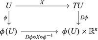
  is differentiable (this is just a standard vector field on $\phi (U) \subset \mathbb{R}^{n}$).

A particularly important set of vector fields is defined by a chart.

Definition A.1.34

Let (U, ϕ) be a chart for M. Then we define at every point p ∈ U the following vectors:

$$\displaystyle{ \frac{\partial } {\partial x_{\mu }}(\,p) = (D_{p}\phi )^{-1}(e_{\mu }),\quad \forall \mu = 1,\ldots,n, }$$

where e ₁, …, e _n is the standard basis of $\mathbb{R}^{n}$. We also write

$$\displaystyle{ \partial _{\mu } = \frac{\partial } {\partial x_{\mu }}. }$$

For a fixed index μ, as p varies, the vectors ∂ _μ ( p) form a smooth vector field ∂ _μ on U. We call the vector fields ∂ _μ basis vector fields or coordinate vector fields on U.

Lemma A.1.35

At each point p ∈ U the vectors ∂ ₁( p), …∂ _n ( p) form a basis for the tangent space T _p M.

Proof

This is clear, because $D_{p}\phi: T_{p}M \rightarrow \mathbb{R}^{n}$ is an isomorphism of vector spaces. □

Proposition A.1.36

Every smooth vector field X on M can be written on U as

$$\displaystyle{ X\vert _{U} =\sum _{ \mu =1}^{n}X^{\mu }\partial _{\mu } \equiv X^{\mu }\partial _{\mu } }$$

where $X^{1},\ldots,X^{n}: U \rightarrow \mathbb{R}$ are smooth real-valued functions on U, called the components of X with respect to the basis {∂ _μ }.

Remark A.1.37

The second equality in this proposition is an example of the so-called Einstein summation convention .

A.1.9 Integral Curves

Let M be a smooth manifold and X a smooth vector field on M.

Definition A.1.38

A curve γ: I → M, where $I \subset \mathbb{R}$ is an open interval around 0, is called an integral curve for X through p ∈ M if

$$\displaystyle{ \gamma (0) = p\quad \text{and}\quad \dot{\gamma }(t) = X_{\gamma (t)}\quad \forall t \in I. }$$

The theory of ordinary differential equations (ODEs) applied in a chart for M shows that:

Theorem A.1.39

For every point q ∈ M there exists an interval I _q around 0 and a unique curve γ _q : I _q → M which is an integral curve for X.

Using a theorem on the behaviour of solutions to ODEs under variation of the initial condition we get:

Theorem A.1.40

For all p ∈ M there exists an open neighbourhood U of p in M and an open interval I around 0 such that the integral curves γ _q are defined on I for all q ∈ U. The map

$$\displaystyle\begin{array}{rcl} \phi _{U}: U \times I& \longrightarrow M & {}\\ (q,t)& \longmapsto \gamma _{q}(t)& {}\\ \end{array}$$

is differentiable and is called the local flow of X.

Theorem A.1.41

Let M be a closed manifold (compact and without boundary). Then there exists a global flow of X which is a smooth map

$$\displaystyle\begin{array}{rcl} \phi: M \times \mathbb{R}& \longrightarrow & M {}\\ (q,t)& \longmapsto & \gamma _{q}(t). {}\\ \end{array}$$

The map

$$\displaystyle{ \phi _{t} =\phi (\cdot,t): M\longrightarrow M }$$

is a diffeomorphism for all $t \in \mathbb{R}$ .

A.1.10 The Commutator of Vector Fields

Let X be a smooth vector field on the manifold M.

Definition A.1.42

The Lie derivative L _X is the map

$$\displaystyle{ L_{X}: \mathcal{C}^{\infty }(M)\longrightarrow \mathcal{C}^{\infty }(M), }$$

defined by

$$\displaystyle{ (L_{X}f)(\,p) = (D_{p}f)(X_{p}) }$$

for all $f \in \mathcal{ C}^{\infty }(M)$ and p ∈ M.

The Lie derivative L _X is the directional derivative of a smooth function along the vector field X: If γ is a curve through p such that $\dot{\gamma }(0) = X_{p}$, then

$$\displaystyle{ (L_{X}f)(\,p) =\dot{ (f\circ \gamma )}(0). }$$

Proposition A.1.43

The Lie derivative is a derivation , i.e. 

• 1. L _X is $\mathbb{R}$ -linear

• 2. L _X satisfies the Leibniz rule :

  $$\displaystyle{ L_{X}(f \cdot g) = (L_{X}f) \cdot g + f \cdot (L_{X}g)\quad \forall f,g \in \mathcal{ C}^{\infty }(M). }$$

Using the Lie derivative we can define the so-called commutator of vector fields.

Theorem A.1.44

Let X and Y be smooth vector fields on M. Then there exists a unique vector field [X, Y ] on M, called the commutator of X and Y, such that

$$\displaystyle{ L_{[X,Y ]} = L_{X} \circ L_{Y } - L_{Y } \circ L_{X}. }$$

(A.1)

If in a local chart (U, ϕ) the vector fields are given by

$$\displaystyle{ X = X^{\mu }\partial _{\mu }\quad \mathit{\text{and}}\quad Y = Y ^{\mu }\partial _{\mu }, }$$

then [X, Y ] is given by

$$\displaystyle{ [X,Y ] = \left (X^{\nu }\frac{\partial Y ^{\mu }} {\partial x^{\nu }} - Y ^{\nu }\frac{\partial X^{\mu }} {\partial x^{\nu }} \right )\partial _{\mu }. }$$

(A.2)

Theorem A.1.45

The set of vector field $\mathfrak{X}(M)$ together with the commutator is an (infinite-dimensional) Lie algebra , i.e. for all $X,Y,Z \in \mathfrak{X}(M)$ we have:

• antisymmetry:

  $$\displaystyle{ [Y,X] = -[X,Y ] }$$

• $\mathbb{R}$ -bilinearity:

  $$\displaystyle{ [aX + bY,Z] = a[X,Z] + b[Y,Z]\quad \forall a,b \in \mathbb{R} }$$

• Jacobi identity :

  $$\displaystyle{ [X,[Y,Z]] + [Y,[Z,X]] + [Z,[X,Y ]] = 0. }$$

We can calculate the commutator [X, Y ] using the flow of X:

Theorem A.1.46

Let X and Y be smooth vector fields on M, ϕ _t the flow of X and p ∈ M a point. Then

$$\displaystyle{ [X,Y ]_{p} = \left. \frac{d} {dt}\right \vert _{t=0}(\phi _{-t})_{{\ast}}Y _{\phi _{t}(\,p)}. }$$

Note that $(\phi _{-t})_{{\ast}}Y _{\phi _{t}(\,p)}$ is a smooth curve in T _p M.

A.1.11 Vector Fields Related by a Smooth Map

Definition A.1.47

Let M and N be smooth manifolds and ϕ: M → N a smooth map. Suppose that X is a vector field on M and Y a vector field on N. Then Y is said to be ϕ -related to X if

$$\displaystyle{ Y _{\phi (\,p)} = (D_{p}\phi )(X_{p})\quad \forall p \in M. }$$

Lemma A.1.48

Let M and N be smooth manifolds, ϕ: M → N a smooth map. Suppose that X and Y are vector fields on M and N and that Y is ϕ-related to X. Then

$$\displaystyle{ (L_{Y }f)\circ \phi = L_{X}(f\circ \phi )\quad \forall f \in \mathcal{ C}^{\infty }(N). }$$

Proposition A.1.49

Let M and N be smooth manifolds and ϕ: M → N a smooth map. Suppose that X′ is ϕ-related to X and Y ′ is ϕ-related to Y. Then [X′, Y ′] is ϕ-related to [X, Y ].

Definition A.1.50

If ϕ: M → N is a diffeomorphism and X is a smooth vector field on M, then we define a smooth vector field ϕ _∗ X on N, called the pushforward of X under ϕ, by

$$\displaystyle{ (\phi _{{\ast}}X)_{\phi (\,p)} = (D_{p}\phi )(X_{p}). }$$

Note that ϕ _∗ X is the unique vector field on N that is ϕ-related to X.

Corollary A.1.51

If ϕ: M → N is a diffeomorphism, then

$$\displaystyle{ [\phi _{{\ast}}X,\phi _{{\ast}}Y ] =\phi _{{\ast}}[X,Y ] }$$

for all vector fields X and Y on M.

A.1.12 Distributions and Foliations

We consider some concepts related to distributions and foliations on manifolds (we follow [142] where proofs and more details can be found). Let M be a smooth manifold of dimension n.

Definition A.1.52

A distribution D of rank k on M is a collection of vector subspaces D _p ⊂ T _p M of dimension k for all p ∈ M which vary smoothly over M, i.e. each p ∈ M has an open neighbourhood U ⊂ M so that D | _U is spanned by k smooth vector fields X ₁, …, X _k on U.

An equivalent definition is that D is a subbundle of rank k of the tangent bundle TM.

Definition A.1.53

A distribution is called involutive or integrable if for all vector fields X, Y on M with X _p , Y _p ∈ D _p for all p ∈ M, the vector field [X, Y ] on M again satisfies [X, Y ] _p ∈ D _p for all p ∈ M.

Definition A.1.54

A foliation $\mathcal{F}$ of rank k on M is a decomposition of M into k-dimensional immersed submanifolds, called leaves, which locally have the following structure: around each point p ∈ M there exists a coordinate neighbourhood diffeomorphic to $\mathbb{R}^{n}$ such that the leaves of the foliation decompose $\mathbb{R}^{n}$ into $\mathbb{R}^{k} \times \mathbb{R}^{n-k}$, with the leaves given by the affine subspaces $\mathbb{R}^{k} \times \{ x\}$ for all $x \in \mathbb{R}^{n-k}$.

It is clear that the tangent spaces to the leaves of a foliation define a distribution. In fact, we have:

Theorem A.1.55 (Frobenius Theorem)

A distribution D defines a foliation $\mathcal{F}$ if and only if D is integrable.

The following statement is Theorem 1.62 in [142].

Theorem A.1.56

Let f: N → M be a smooth map between manifolds, $\mathcal{H}$ a foliation on M and H ⊂ M a leaf of $\mathcal{H}$ . Suppose that f has image in H. Then f: N → H is smooth.

This theorem is clear if H is an embedded submanifold of M and only non-trivial if H is an immersed submanifold.

A.2 Tensors and Forms

A.2.1 Tensors and Exterior Algebra of Vector Spaces

We recall some notions from linear algebra. Let V denote an n-dimensional real vector space.

Definition A.2.1

We set

$$\displaystyle{ V ^{{\ast}} =\{\lambda \mid \lambda: V \rightarrow \mathbb{R}\text{ is linear}\} }$$

for the dual space of V. The dual space V ^∗ is itself an n-dimensional real vector space. We call the elements λ ∈ V ^∗ 1-forms on V.

If {e _μ } is a basis for V we get a dual basis {ω ^ν} for V ^∗ defined by

$$\displaystyle{ \omega ^{\nu }(e_{\mu }) =\delta _{ \mu }^{\nu },\quad \forall \mu,\nu = 1,\ldots,n, }$$

where δ _μ ^ν is the standard Kronecker delta. Just as we decompose any vector X ∈ V in the basis {e _μ } as

$$\displaystyle{ X = X^{\mu }e_{\mu } }$$

we can decompose any 1-form λ ∈ V ^∗ as

$$\displaystyle{ \lambda =\lambda _{\nu }\omega ^{\nu }. }$$

(Note the Einstein summation convention in both cases.)

Definition A.2.2

A tensor of type (l, k) is a multilinear map

$$\displaystyle{ T: \mathop{\underbrace{V ^{{\ast}}\times \cdots \times V ^{{\ast}}}}\limits _{l} \times \mathop{\underbrace{ V \times \cdots \times V }}\limits _{k}\longrightarrow \mathbb{R}. }$$

In particular, a (0, 1)-tensor is a 1-form and a (1, 0)-tensor is a vector. The set of all (l, k)-tensors forms a vector space.

We are interested in a particular class of tensors on a vector space V.

Definition A.2.3

We call a (0, k)-tensor

$$\displaystyle{ \lambda: \mathop{\underbrace{V \times \cdots \times V }}\limits _{k}\longrightarrow \mathbb{R} }$$

a k-form on V if λ is alternating , i.e. totally antisymmetric:

$$\displaystyle{ \lambda (\ldots,v,\ldots,w,\ldots ) = -\lambda (\ldots,w,\ldots,v,\ldots ) }$$

for all insertions of vectors into λ, where only the vectors v and w are interchanged. The set of k-forms on V forms a vector space denoted by Λ ^k V ^∗.

Remark A.2.4

It follows that for k-forms λ

$$\displaystyle{ \lambda (\ldots,v,\ldots,v,\ldots ) = 0\quad \forall v \in V }$$

and

$$\displaystyle{ \lambda (v_{1},v_{2},\ldots,v_{k}) = 0 }$$

whenever the vectors v ₁, v ₂, …, v _k are linearly dependent. In particular, every k-form on V vanishes identically if k is larger than the dimension of V.

Definition A.2.5

Let λ be a k-form and μ an l-form. Then the wedge product of λ ∧μ is the (k + l)-form defined by

$$\displaystyle\begin{array}{rcl} & & (\lambda \wedge \mu )(X_{1},\ldots,X_{k+l}) {}\\ & & \quad = \frac{1} {k!l!}\sum _{\sigma \in S_{k+l}}\mathrm{sgn}(\sigma )\lambda \left (X_{\sigma (1)},\ldots,X_{\sigma (k)}\right ) \cdot \mu \left (X_{\sigma (k+1)},\ldots,X_{\sigma (k+l)}\right ). {}\\ \end{array}$$

Here S _k+l denotes the set of permutations of {1, 2, …, k + l}. It can be checked that λ ∧μ is indeed a k + l-form.

Example A.2.6

Let α, β be 1-forms on V. Then

$$\displaystyle{ (\alpha \wedge \beta )(X,Y ) =\alpha (X)\beta (Y ) -\alpha (Y )\beta (X) }$$

for all vectors X, Y ∈ V.

Lemma A.2.7

Let V be a vector space of dimension n and {ω ^ν} a basis for V ^∗ . Then the set of k-forms

$$\displaystyle{ \omega ^{\nu _{1}} \wedge \cdots \wedge \omega ^{\nu _{k}},\mathit{\text{ with }}1 \leq \nu _{1} <\nu _{2} <\ldots <\nu _{k} \leq n, }$$

is a basis for the vector space of k-forms.

A.2.2 Tensors and Differential Forms on Manifolds

Let M be an n-dimensional smooth manifold. We want to extend the notion of tensors and forms on vector spaces to tensors and forms on M. One possibility is to first define certain vector bundles and then tensors and forms as smooth sections of these bundles. However, since we define vector bundles in Sect. 4.5, we use here another, equivalent definition for tensors.

Remark A.2.8

In the following all functions and vector fields on M are smooth.

Definition A.2.9

We denote by $\mathcal{C}^{\infty }(M)$ the ring of all smooth functions $f: M \rightarrow \mathbb{R}$. We also denote by $\mathfrak{X}(M)$ the set of all smooth vector fields on M. The set $\mathfrak{X}(M)$ is a real vector space and module over $\mathcal{C}^{\infty }(M)$ by point-wise multiplication.

We can now define:

Definition A.2.10

A 1-form λ on the manifold M is a map

$$\displaystyle{ \lambda: \mathfrak{X}(M)\longrightarrow \mathcal{C}^{\infty }(M) }$$

that is linear over $\mathcal{C}^{\infty }(M)$, i.e. 

$$\displaystyle\begin{array}{rcl} \lambda (X + Y )& =& \lambda (X) +\lambda (Y ), {}\\ \lambda (f \cdot X)& =& f \cdot \lambda (X) {}\\ \end{array}$$

for all vector fields $X,Y \in \mathfrak{X}(M)$ and functions $f \in \mathcal{ C}^{\infty }(M)$. We denote the set of all 1-forms on M by Ω ¹(M), which is a real vector space and module over $\mathcal{C}^{\infty }(M)$.

The following can be proved:

Proposition A.2.11

The value of λ(X)( p) for a 1-form λ and vector field X at a point p ∈ M depends only on X _p . Hence if Y is another vector field on M with Y _p = X _p , then λ(X)( p) = λ(Y )( p).

A proof of this proposition can be found in [142, p. 64]. Similarly we set:

Definition A.2.12

A tensor T of type (l, k) on M is a map

$$\displaystyle{ T: \mathop{\underbrace{\varOmega ^{1}(M) \times \cdots \times \varOmega ^{1}(M)}}\limits _{l} \times \mathop{\underbrace{ \mathfrak{X}(M) \times \cdots \times \mathfrak{X}(M)}}\limits _{k}\longrightarrow \mathcal{C}^{\infty }(M) }$$

that is $\mathcal{C}^{\infty }(M)$-linear in each entry. A k -form or differential form ω on M is a (0, k)-tensor

$$\displaystyle{ \omega: \mathop{\underbrace{\mathfrak{X}(M) \times \cdots \times \mathfrak{X}(M)}}\limits _{k}\longrightarrow \mathcal{C}^{\infty }(M) }$$

that is in addition alternating (totally antisymmetric). We denote the set of k-forms on M by Ω ^k(M).

Remark A.2.13

An argument similar to the proof of Proposition A.2.11 shows that tensors and k-forms on manifolds have well-defined values at every point p ∈ M. We can therefore insert, for example, in a k-form ω ∈ Ω ^k(M) vectors X ₁, …, X _k in the tangent space T _p M at any point p ∈ M and get a real number. We can also speak unambiguously of the value of a tensor or form at a point.

Remark A.2.14

We can define the wedge product ∧ of forms as before by replacing in the definition vectors by vector fields on the manifold. The wedge product is then a map

$$\displaystyle{ \wedge: \varOmega ^{k}(M) \times \varOmega ^{l}(M)\longrightarrow \varOmega ^{k+l}(M). }$$

A.2.3 Scalar Products and Metrics on Manifolds

We consider the following definition from linear algebra.

Definition A.2.15

A scalar product on the vector space V is a symmetric non-degenerate (0, 2)-tensor g on V:

$$\displaystyle\begin{array}{rcl} g(v,w)& =& g(w,v)\quad \forall v,w \in V \quad \text{(symmetric)} {}\\ g(v,\cdot )& \neq & 0 \in V ^{{\ast}}\quad \forall v\neq 0 \in V \quad \text{(non-degenerate)}. {}\\ \end{array}$$

The scalar product g is called Euclidean if it is positive definite

$$\displaystyle\begin{array}{rcl} g(v,v)& \geq & 0\quad \forall v \in V {}\\ g(v,v)&>& 0\quad \forall v\neq 0 {}\\ \end{array}$$

and pseudo-Euclidean otherwise.

We can do the same construction on manifolds.

Definition A.2.16

A metric on a smooth manifold M is a (0, 2)-tensor g which is a scalar product at each point p ∈ M. The metric is called Riemannian if the scalar products g _p are Euclidean and pseudo-Riemannian if the scalar products g _p are pseudo-Euclidean, for all p ∈ M.

It can be shown using partitions of unity that every smooth manifold admits a Riemannian metric (but not necessarily a pseudo-Riemannian metric).

A.2.4 The Levi-Civita Connection

Let (M, g) be a pseudo-Riemannian manifold. The Levi-Civita connection is a metric and torsion-free, covariant derivative on the tangent bundle of the manifold, i.e. a map

$$\displaystyle\begin{array}{rcl} \nabla: \mathfrak{X}(M) \times \mathfrak{X}(M)& \longrightarrow & \mathfrak{X}(M) {}\\ (X,Y )& \longmapsto & \nabla _{X}Y {}\\ \end{array}$$

with the following properties:

• 1. ∇ is $\mathbb{R}$-linear in both X and Y.

• 2. ∇ is $\mathcal{C}^{\infty }(M)$-linear in X and satisfies

  $$\displaystyle{ \nabla _{X}(fY ) = (L_{X}f)Y + f\nabla _{X}Y \quad \forall f \in \mathcal{ C}^{\infty }(M),X,Y \in \mathfrak{X}(M). }$$

• 3. ∇ is metric, i.e. 

  $$\displaystyle{ L_{X}g(Y,Z) = g(\nabla _{X}Y,Z) + g(Y,\nabla _{X}Z)\quad \forall X,Y,Z \in \mathfrak{X}(M). }$$

• 4. ∇ is torsion-free, i.e. 

  $$\displaystyle{ \nabla _{X}Y -\nabla _{Y }X = [X,Y ]\quad \forall X,Y \in \mathfrak{X}(M). }$$

The Levi-Civita connection can be calculated with the following Koszul formula :

$$\displaystyle\begin{array}{rcl} 2g(\nabla _{X}Y,Z)& =& L_{X}g(Y,Z) + L_{Y }g(X,Z) - L_{Z}g(X,Y ) {}\\ & & -g([X,Z],Y ) - g([Y,Z],X) + g([X,Y ],Z). {}\\ \end{array}$$

A.2.5 Coordinate Representations

We saw above that we can represent every vector field X on a chart neighbourhood U by X | _U = X ^μ ∂ _μ , where X ^μ are certain functions on U, called components. We want to decompose in a similar way tensors and forms on U. In the physics literature tensors and forms are often given in terms of their components in coordinate systems.

Definition A.2.17

Let U be a chart neighbourhood. We define the set of dual 1-forms dx ^μ, for μ = 1, …, n, by dx ^μ(∂ _ν ) = δ _ν ^μ at each point p ∈ U.

Proposition A.2.18

Let λ be a 1-form on M. Then we can decompose λ on U as λ | _U = λ _μ dx ^μ for certain smooth functions λ _μ on M. Similarly, we can decompose a k-form ω as

$$\displaystyle{ \omega \vert _{U} =\sum _{1\leq \nu _{1}<\cdots <\nu _{k}\leq n}\omega _{\nu _{1}\ldots \nu _{k}}dx^{\nu _{1}} \wedge \cdots \wedge dx^{\nu _{k}}, }$$

with smooth functions $\omega _{\nu _{1}\ldots \nu _{k}}$ .

Note that these functions, corresponding to the components, depend on the choice of the chart (U, ϕ), while the objects themselves (vectors fields, k-forms) are independent of charts.

A.2.6 The Pullback of Forms on Manifolds

Let ω ∈ Ω ^k(N) be a k-form on a manifold N and f: M → N a smooth map.

Definition A.2.19

The pullback of ω under f is the k-form f ^∗ ω ∈ Ω ^k(M) on M defined by

$$\displaystyle{ (f^{{\ast}}\omega )(X_{ 1},\ldots,X_{k}) =\omega (f_{{\ast}}X_{1},\ldots,f_{{\ast}}X_{k}) }$$

for all tangent vectors X ₁, …, X _k ∈ T _p M and all p ∈ M.

Proposition A.2.20

The pullback defines a map f ^∗: Ω ^k(N) ⟶ Ω ^k(M). We have

$$\displaystyle{ f^{{\ast}}(\omega \wedge \eta ) = (f^{{\ast}}\omega ) \wedge (f^{{\ast}}\eta ) }$$

for all ω ∈ Ω ^k(N), η ∈ Ω ^l(N) and

$$\displaystyle{ (g \circ f)^{{\ast}} = f^{{\ast}}\circ g^{{\ast}} }$$

for all smooth maps f: M → N, g: N → Q.

The second property follows from the chain rule for the differential of the map g ∘ f.

A.2.7 The Differential of Forms on Manifolds

The differential is a very important map on forms on a manifold that raises the degree by one.

Theorem A.2.21

Let M be a smooth manifold. Then there is a unique map

$$\displaystyle{ d: \varOmega ^{k}(M)\longrightarrow \varOmega ^{k+1}(M) }$$

for every k ≥ 0, called the differential or exterior derivative , that satisfies the following properties:

• 1. d is $\mathbb{R}$ -linear.

• 2. For a function $f \in \varOmega ^{0}(M) =\mathcal{ C}^{\infty }(M)$ and a vector field $X \in \mathfrak{X}(M)$ we have df(X) = L _X f.

• 3. d ² = d ∘ d = 0: Ω ^k(M) → Ω ^k+2(M).

• 4. d satisfies the following Leibniz rule :

  $$\displaystyle{ d(\alpha \wedge \beta ) = d\alpha \wedge \beta +(-1)^{k}\alpha \wedge d\beta }$$

  for all α ∈ Ω ^k(M), β ∈ Ω ^l(M).

The proof of this fundamental theorem can be found in any book on differential geometry. Let (U, ϕ) be a local chart. If we assume that the differential d has these properties, then it follows that the differential is given on functions f by

$$\displaystyle{ df = \frac{\partial f} {\partial x^{\nu }}dx^{\nu } }$$

and on Ω ^k(M) by

$$\displaystyle\begin{array}{rcl} d\omega & =& d\sum _{1\leq \mu _{1}<\ldots <\mu _{k}\leq n}\omega _{\mu _{1}\ldots \mu _{k}}dx^{\mu _{1}} \wedge \cdots dx^{\mu _{k}} {}\\ & =& \sum _{1\leq \mu _{1}<\ldots <\mu _{k}\leq n}\sum _{\nu =1}^{n}\frac{\partial \omega _{\mu _{1}\ldots \mu _{k}}} {\partial x^{\nu }} dx^{\nu } \wedge dx^{\mu _{1}} \wedge \cdots dx^{\mu _{k}}. {}\\ \end{array}$$

The defining properties of the differential d imply for 1-forms and 2-forms:

Proposition A.2.22

• 1. Let α ∈ Ω ¹(M) be a 1-form. Then

  $$\displaystyle{ d\alpha (X,Y ) = L_{X}(\alpha (Y )) - L_{Y }(\alpha (X)) -\alpha ([X,Y ])\quad \forall X,Y \in \mathfrak{X}(M). }$$

• 2. Let β ∈ Ω ²(M) be a 2-form. Then

  $$\displaystyle\begin{array}{rcl} d\beta (X,Y,Z)& =& L_{X}(\beta (Y,Z)) + L_{Y }(\beta (Z,X)) + L_{Z}(\beta (X,Y )) {}\\ & & -\beta ([X,Y ],Z) -\beta ([Y,Z],X) -\beta ([Z,X],Y )\quad \forall X,Y,Z \in \mathfrak{X}(M). {}\\ \end{array}$$

The differential is natural under pullback:

Proposition A.2.23

If f: M → N is a smooth map and ω ∈ Ω ^k(N), then d(f ^∗ ω) = f ^∗ dω.

Let M be a compact oriented n-dimensional manifold and σ ∈ Ω ⁿ(M) a form of top degree. Then there is a well-defined integral

$$\displaystyle{ \int _{M}\sigma \in \mathbb{R}. }$$

The integral can also be defined if M is non-compact and σ has compact support.

Theorem A.2.24 (Stokes’ Theorem)

 

• 1. Let M be a compact n-dimensional oriented manifold with boundary ∂M and ω ∈ Ω ⁿ⁻¹(M). Then (with a suitable orientation of the boundary)

  $$\displaystyle{ \int _{M}d\omega =\int _{\partial M}\omega. }$$

• 2. Let M be an n-dimensional oriented manifold (not necessarily compact) without boundary and ω ∈ Ω ⁿ⁻¹(M) an (n − 1)-form with compact support. Then

  $$\displaystyle{ \int _{M}d\omega = 0. }$$

References

Abe, K. et al. (The T2K Collaboration): First combined analysis of neutrino and antineutrino oscillations at T2K. arXiv:1701.00432
Adams, J.F.: On the non-existence of elements of Hopf invariant one. Ann. Math. 72, 20–104 (1960)
Adams, J.F.: Vector fields on spheres. Ann. Math. 75, 603–632 (1962)
Argyres, P.C.: An introduction to global supersymmetry. Lecture notes, Cornell University 2001. Available at http://homepages.uc.edu/~argyrepc/cu661-gr-SUSY/index.html
Atiyah, M.F.: K-Theory. Notes by D.W. Anderson. W.A. Benjamin, New York/Amsterdam (1967)
Atiyah, M.F., Bott, R.: The Yang–Mills equations over Riemann surfaces. Phil. Trans. R. Soc. Lond. A 308, 523–615 (1983)
Atiyah, M.F., Bott, R., Shapiro, A.: Clifford modules. Topology 3, 3–38 (1964)
Baez, J.C.: The octonions. Bull. Am. Math. Soc. (N.S.) 39, 145–205 (2002); Erratum: Bull. Am. Math. Soc. (N.S.) 42, 213 (2005)
Baez, J., Huerta, J.: The algebra of grand unified theories. Bull. Am. Math. Soc. (N.S.) 47, 483–552 (2010)
Bailin, D., Love, A.: Introduction to Gauge Field Theory. Institute of Physics Publishing, Bristol/Philadelphia (1993)
Ball. P.: Nuclear masses calculated from scratch. Nature, published online 20 November 2008. doi:10.1038/news.2008.1246
Barut, A.O., Raczka, R.: Theory of Group Representations and Applications. Polish Scientific Publishers, Warszawa (1980)
Baum, H.: Spin-Strukturen und Dirac-Operatoren über pseudoriemannschen Mannigfaltigkeiten. Teubner Verlagsgesellschaft, Leipzig (1981)
Baum, H.: Eichfeldtheorie. Springer, Berlin/Heidelberg (2014)
Berline, N., Getzler, E., Vergne, M.: Heat Kernels and Dirac Operators. Springer, Berlin/Heidelberg (2004)
Bleecker, D.: Gauge Theory and Variational Principles. Addison-Wesley Publishing Company, Reading, MA (1981)
Bogolubov, N.N., Logunov, A.A., Todorov, I.T.: Introduction to Axiomatic Quantum Field Theory. W. A. Benjamin, Reading, MA (1975)
Borsanyi, Sz. et al: Ab initio calculation of the neutron-proton mass difference. Science 347(6229), 1452–1455 (2015)
Bott, M.R.: An application of the Morse theory to the topology of Lie-groups, Bull. Soc. Math. France 84, 251–281 (1956)
Bourguignon, J.-P., Hijazi, O., Milhorat, J.-L., Moroianu, A., Moroianu, S.: A Spinorial Approach to Riemannian and Conformal Geometry. European Mathematical Society, Zürich (2015)
Brambilla, N. et al.: QCD and strongly coupled gauge theories: challenges and perspectives. Eur. Phys. J. C 74, 2981 (2014)
Branco, G.C., Lavoura, L., Silva, J.P.: CP Violation. Oxford University Press, Oxford (1999)
Bredon, G.E.: Introduction to Compact Transformation Groups. Academic Press, New York/London (1972)
Bröcker, T., tom Dieck, T.: Representations of Compact Lie Groups. Springer, Berlin/Heidelberg/New York (2010)
Bröcker, T., Jänich, K.: Einführung in die Differentialtopologie. Springer, Berlin/Heidelberg/New York (1990)
Bryant, R.L.: Metrics with exceptional holonomy. Ann. Math. 126, 525–576 (1987)
Bryant, R.L.: Submanifolds and special structures on the octonians. J. Differ. Geom. 17, 185–232 (1982)
Budinich, R., Trautman, A.: The Spinorial Chessboard. Springer, Berlin/Heidelberg (1988)
Bueno, A. et al.: Nucleon decay searches with large liquid Argon TPC detectors at shallow depths: atmospheric neutrinos and cosmogenic backgrounds. JHEP 0704, 041 (2007)
Čap, A., Slovák, J.: Parabolic Geometries I: Background and General Theory. American Mathematical Society, Providence, RI (2009)
CERN Press Release: CERN experiments observe particle consistent with long-sought Higgs boson. Available at http://press.cern/press-releases/2012/07/cern-experiments-observe-particle-consistent-long-sought-higgs-boson
Chaichian, M., Nelipa, N.F.: Introduction to Gauge Field Theories. Springer, Berlin/Heidelberg/New York/Tokyo (1984)
Cheng, T.-P., Li, L.-F.: Gauge Theory of Elementary Particle Physics. Oxford University Press, Oxford (1988)
Chevalley, C.: Theory of Lie Groups I. Princeton University Press, Princeton (1946)
Chevalley, C.: The Algebraic Theory of Spinors and Clifford Algebras. Collected Works, Vol. 2. Springer, Berlin/Heidelberg (1997)
Chivukula, R.S.: The origin of mass in QCD. arXiv:hep-ph/0411198
Clay Mathematics Institute: Millenium problems. Yang–Mills and mass gap. Available at http://www.claymath.org/millennium-problems/yang--mills-and-mass-gap
Costello, K.: Renormalization and Effective Field Theory. Mathematical Surveys and Monographs, Vol. 170. American Mathematical Society, Providence, RI (2011)
Darling, R.W.R.: Differential Forms and Connections. Cambridge University Press, Cambridge (1994)
D’Auria, R., Ferrara, S., Lledó, M.A., Varadarajan, V.S.: Spinor algebras. J. Geom. Phys. 40, 101–129 (2001)
Derdzinski, A.: Geometry of the Standard Model of Elementary Particles. Springer, Berlin/Heidelberg (1992)
Dissertori, G., Knowles, I., Schmelling, M.: Quantum Chromodynamics. High Energy Experiments and Theory. Oxford University Press, Oxford (2003)
Drexlin, G., Hannen, V., Mertens, S., Weinheimer, C.: Current direct neutrino mass experiments. Adv. High Energy Phys. 2013, Article ID 293986 (2013)
Dürr, S. et al.: Ab initio determination of light hadron masses. Science 322, 1224–1227 (2008)
Duncan, A.: The Conceptual Framework of Quantum Field Theory. Oxford University Press, Oxford (2013)
Dynkin, E.B.: Semisimple subalgebras of the semisimple Lie algebras. (Russian) Mat. Sbornik 30, 349–462 (1952); English translation: Am. Math. Soc. Transl. Ser. 2 6, 111–244 (1957)
Elliott, C.: Gauge Theoretic Aspects of the Geometric Langlands Correspondence. Ph.D. Thesis, Northwestern University (2016)
Englert, F., Brout R.: Broken symmetry and the mass of gauge vector mesons. Phys. Rev. Lett. 13, 321–323 (1964)
Figueroa-O’Farrill, J.: Majorana Spinors. Lecture Notes. University of Edinburgh (2015)
Flory, M., Helling, R.C., Sluka, C.: How I learned to stop worrying and love QFT. arXiv:1201.2714 [math-ph]
Folland, G.B.: Quantum Field Theory. A Tourist Guide for Mathematicians. American Mathematical Society, Providence, Rhodes Island (2008)
Freed, D.S.: Classical Chern–Simons theory, 1. Adv. Math. 113, 237–303 (1995)
Freed, D.S.: Five Lectures on Supersymmetry. American Mathematical Society, Providence, RI (1999)
Freedman, D.Z., Van Proeyen, A.: Supergravity. Cambridge University Press, Cambridge (2012)
Friedrich, T.: Dirac Operators in Riemannian Geometry. American Mathematical Society, Providence, RI (2000)
Fritzsch, H., Minkowski, P.: Unified interactions of leptons and hadrons. Ann. Phys. 93, 193–266 (1975)
Geiges, H.: An Introduction to Contact Topology. Cambridge University Press, Cambridge (2008)
Georgi, H.: The state of the art – gauge theories. In: Carlson, C.E. (ed.) Particles and Fields – 1974: Proceedings of the Williamsburg Meeting of APS/DPF, pp. 575–582. AIP, New York (1975)
Georgi, H., Glashow, S.L.: Unity of all elementary-particle forces. Phys. Rev. Lett. 32, 438–441 (1974)
Georgi, H.M., Glashow, S.L., Machacek, M.E., Nanopoulos, D.V.: Higgs Bosons from two-gluon annihilation in proton-proton collisions. Phys. Rev. Lett. 40 692 (1978)
Georgi, H., Quinn, H.R., Weinberg, S.: Hierarchy of interactions in unified gauge theories. Phys. Rev. Lett. 33, 451–454 (1974)
Giunti, C., Kim, C.W.: Fundamentals of Neutrino Physics and Astrophysics. Oxford University Press, Oxford (2007)
Glashow, S.L.: Trinification of all elementary particle forces. In: 5th Workshop on Grand Unification, Providence, RI, April 12–14, 1984
Glashow, S.L., Iliopoulos, J., Maiani, L.: Weak interactions with lepton-hadron symmetry. Phys. Rev. D 2, 1285–1292 (1970)
Gleason, A.M.: Groups without small subgroups. Ann. Math. 56, 193–212 (1952)
Grimus, W., Rebelo, M.N.: Automorphisms in gauge theories and the definition of CP and P. Phys. Rep. 281, 239–308 (1997)
Guralnik, G.S., Hagen, C.R., Kibble, T.W.B.: Global conservation laws and massless particles. Phys. Rev. Lett. 13, 585–587 (1964)
Gürsey, F., Ramond, P., Sikivie, P.: A universal gauge theory model based on E6. Phys. Lett. B 60, 177–180 (1976)
Haag, R.: Local Quantum Physics. Fields, Particles, Algebras. Springer, Berlin/ Heidelberg/New York (1996)
Hall, B.C.: Lie Groups, Lie Algebras and Representations. An Elementary Introduction. Springer, Cham Heidelberg/New York/Dordrecht/London (2016)
Halzen, F., Martin, A.D.: Quarks and Leptons. An Introductory Course in Modern Particle Physics. Wiley, New York/Chichester/Brisbane/Toronto/Singapore (1984)
Hartanto, A., Handoko L.T.: Grand unified theory based on the SU(6) symmetry. Phys. Rev. D 71, 095013 (2005)
Harvey, R., Lawson, H.B.: Calibrated geometries. Acta Math. 148, 47–157 (1982)
Hatcher, A.: Vector bundles and K-theory. Version 2.1, May 2009
Heeck, J.: Interpretation of lepton flavor violation. Phys. Rev. D 95, 015022 (2017)
Higgs, P.W.: Broken symmetries and the masses of gauge bosons. Phys. Rev. Lett. 13, 508–509 (1964)
Hilgert, J., Neeb, K.-H.: Structure and Geometry of Lie Groups. Springer, New York/ Dordrecht/Heidelberg/London (2012)
Hirsch, M.W.: Differential Topology. Springer, New York/Berlin/Heidelberg (1997)
Hoddeson, L., Brown, L., Riordan, M., Dresden, M. (ed.): The Rise of the Standard Model: Particle Physics in the 1960s and 1970s. Cambridge University Press, Cambridge (1997)
Hollowood, T.J.: Renormalization Group and Fixed Points in Quantum Field Theory. Springer, Heidelberg/New York/Dordrecht/London (2013)
Husemoller, D.: Fibre Bundles. Springer, New York (1994)
Klaczynski, L.: Haag’s Theorem in renormalisable quantum field theory. Ph.D. Thesis, Humboldt Universität zu Berlin (2015)
Knapp, A.W.: Lie Groups Beyond an Introduction. Birkhäuser, Boston/Basel/Berlin (2002)
Kobayashi, S., Nomizu, K.: Foundations of Differential Geometry, Vol. I. Interscience Publishers, New York/London (1963)
Kounnas, C., Masiero, A., Nanopoulos, D.V., Olive, K.A.: Grand Unification with and Without Supersymmetry and Cosmological Implications. World Scientific, Singapore (1984)
Lancaster, T., Blundell, S. J.: Quantum Field Theory for the Gifted Amateur. Oxford University Press, Oxford (2014)
Langacker, P.: Grand unified theories and proton decay. Phys. Rep. 72, 185–385 (1981)
Lawson, H.B. Jr., Michelsohn, M.-L.: Spin Geometry. Princeton University Press, Princeton, NJ (1989)
Lee, J.M.: Introduction to Smooth Manifolds. Springer, New York/Heidelberg/Dordrecht/ London (2013)
Leigh, R.G., Strassler, M.J.: Duality of Sp(2N c ) and SO(N c ) supersymmetric gauge theories with adjoint matter. Phys. Lett. B 356, 492–499 (1995)
Martin, S.P.: A supersymmetry primer. arXiv:hep-ph/9709356
Mayer, M.E.: Review: David D. Bleecker, Gauge theory and variational principles. Bull. Am. Math. Soc. (N.S.) 9, 83–92 (1983)
Meinrenken, E.: Clifford Algebras and Lie Theory. Springer, Berlin/Heidelberg (2013)
Milnor, J.: On manifolds homeomorphic to the 7-sphere. Ann. Math. 64, 399–405 (1956)
Misner, C.W., Thorne, K.S., Wheeler, J.A.: Gravitation. W. H. Freeman and Company, New York (1973)
Mohapatra, R.N.: Unification and Supersymmetry. The Frontiers of Quark-Lepton Physics. Springer, New York/Berlin/Heidelberg (2003)
Montgomery, D., Zippin, L.: Small subgroups of finite-dimensional groups. Ann. Math. 56, 213–241 (1952)
Moore, J.D.: Lectures on Seiberg–Witten Invariants. Springer, Berlin/Heidelberg/New York (2001)
Morgan, J.W.: The Seiberg–Witten Equations and Applications to the Topology of Smooth Four-Manifolds. Princeton University Press, Princeton, NJ (1996)
Mosel, U.: Fields, Symmetries, and Quarks. Springer, Berlin/Heidelberg (1999)
Naber, G.L.: Topology, Geometry and Gauge Fields. Foundations. Springer, New York (2011)
Naber, G.L.: Topology, Geometry and Gauge Fields. Interactions. Springer, New York (2011)
Nakahara, M.: Geometry, Topology and Physics, 2nd edn. IOP Publishing Ltd, Bristol/ Philadelphia (2003)
O’Raifeartaigh, L.: Group Structure of Gauge Theories. Cambridge University Press, Cambridge (1986)
Patrignani, C. et al. (Particle Data Group): 2016 Review of particle physics. Chin. Phys. C 40, 100001 (2016). http://www-pdg.lbl.gov/
Patrignani, C. et al. (Particle Data Group): 2016 Review of particle physics. Particle listings. Chin. Phys. C 40, 100001 (2016). http://www-pdg.lbl.gov/
Patrignani, C. et al. (Particle Data Group): 2016 Review of particle physics. Particle listings. Neutrino mixing. Chin. Phys. C 40, 100001 (2016). http://www-pdg.lbl.gov/
Patrignani, C. et al. (Particle Data Group): 2016 Review of particle physics. Reviews, tables, and plots. 1. Physical constants. Chin. Phys. C 40, 100001 (2016). http://www-pdg.lbl.gov/
Patrignani, C. et al. (Particle Data Group): 2016 Review of particle physics. Reviews, tables, and plots. 10. Electroweak model and constraints on new physics. Chin. Phys. C 40, 100001 (2016). http://www-pdg.lbl.gov/
Patrignani, C. et al. (Particle Data Group): 2016 Review of particle physics. Reviews, tables, and plots. 12. The CKM quark-mixing matrix. Chin. Phys. C 40, 100001 (2016). http://www-pdg.lbl.gov/
Patrignani, C. et al. (Particle Data Group): 2016 Review of particle physics. Reviews, tables, and plots. 16. Grand unified theories. Chin. Phys. C 40, 100001 (2016). http://www-pdg.lbl.gov/
Pich, A.: The Standard Model of electroweak interactions. arXiv:1201.0537 [hep-ph]
Quigg, C.: Gauge Theories of the Strong, Weak, and Electromagnetic Interactions. Westview Press, Boulder, Colorado (1997)
Robinson, M.: Symmetry and the Standard Model. Mathematics and Particle Physics. Springer, New York/Dordrecht/Heidelberg/London (2011)
Roe, J.: Elliptic Operators, Topology and Asymptotic Methods. Longman Scientific & Technical, Harlow (1988)
Roman, P.: Introduction to Quantum Field Theory. Wiley, New York/London/Sydney/Toronto (1969)
Royal Swedish Academy of Sciences: The official web site of the nobel prize. https://www.nobelprize.org/nobel_prizes/physics/
Royal Swedish Academy of Sciences: Asymptotic freedom and quantum chromodynamics: the key to the understanding of the strong nuclear forces. Advanced information on the Nobel Prize in Physics, 5 October 2004. https://www.nobelprize.org/nobel_prizes/physics/laureates/2004/advanced.html
Royal Swedish Academy of Sciences: Class of Physics. Broken symmetries. Scientific Background on the Nobel Prize in Physics 2008. https://www.nobelprize.org/nobel_prizes/physics/laureates/2008/advanced.html
Royal Swedish Academy of Sciences: Class of Physics. The BEH-mechanism, interactions with short range forces and scalar particles. Scientific Background on the Nobel Prize in Physics 2013. https://www.nobelprize.org/nobel_prizes/physics/laureates/2013/advanced.html
Royal Swedish Academy of Sciences: Class of Physics. Neutrino oscillations. Scientific Background on the Nobel Prize in Physics 2015. https://www.nobelprize.org/nobel_prizes/physics/laureates/2015/advanced.html
Rudolph, G., Schmidt, M.: Differential Geometry and Mathematical Physics. Part I. Manifolds, Lie Groups and Hamiltonian Systems. Springer Netherlands, Dordrecht (2013)
Rudolph, G., Schmidt, M.: Differential Geometry and Mathematical Physics. Part II. Fibre Bundles, Topology and Gauge Fields. Springer Netherlands, Dordrecht (2017)
Ryder, L.H.: Quantum Field Theory. Cambridge University Press, Cambridge (1996)
Schwartz, M.D.: Quantum Field Theory and the Standard Model. Cambridge University Press, Cambridge (2014)
Seiberg, N.: Five dimensional SUSY field theories, non-trivial fixed points and string dynamics. Phys. Lett. B 388, 753–760 (1996)
Seiberg, N., Witten, E.: Electric-magnetic duality, monopole condensation, and confinement in N = 2 supersymmetric Yang–Mills theory. Nucl. Phys. B 426, 19–52 (1994). Erratum: Nucl. Phys. B 430, 485–486 (1994)
Seiberg, N., Witten, E.: Monopoles, duality and chiral symmetry breaking in N = 2 supersymmetric QCD. Nucl. Phys. B 431, 484–550 (1994)
Sepanski, M.R.: Compact Lie Groups. Springer Science+Business Media LLC, New York (2007)
Serre, J.-P.: Lie Algebras and Lie Groups. 1964 Lectures given at Harvard University. Springer, Berlin/Heidelberg (1992)
Slansky, R.: Group theory for unified model building. Phys. Rep. 79, 1–128 (1981)
Srednicki, M.: Quantum Field Theory. Cambridge University Press, Cambridge (2007)
Steenrod, N.: The Topology of Fibre Bundles. Princeton University Press, Princeton (1951)
Streater, R.F., Wightman, A.S.: PCT, Spin and Statistics, and All That. Princeton University Press, Princeton, NJ (2000)
Tao, T.: Hilbert’s Fifth Problem and Related Topics. Graduate Studies in Mathematics, Vol. 153. American Mathematical Society, Providence, RI (2014)
Taubes, C.H.: Differential Geometry. Bundles, Connections, Metrics and Curvature. Oxford University Press, Oxford (2011)
Thomson, M.: Modern Particle Physics. Cambridge University Press, Cambridge (2013)
Vafa, C., Zwiebach, B.: N = 1 dualities of SO and USp gauge theories and T-duality of string theory. Nucl. Phys. B 506, 143–156 (1997)
van den Ban, E.P.: Notes on quotients and group actions. Fall 2006. Universiteit Utrecht
Van Proeyen, A.: Tools for supersymmetry. arXiv:hep-th/9910030
van Vulpen, I.: The Standard Model Higgs boson. Part of the Lecture Particle Physics II, University of Amsterdam Particle Physics Master 2013–2014
Warner, F.W.: Foundations of Differentiable Manifolds and Lie Groups. Springer, New York (2010)
Weinberg, S.: The Quantum Theory of Fields, Vol. I. Foundations. Cambridge University Press, Cambridge (1995)
Weinberg, S.: The Quantum Theory of Fields, Vol. II. Modern Applications. Cambridge University Press, Cambridge (1996)
Weinberg, S.: The Quantum Theory of Fields, Vol. III. Supersymmetry. Cambridge University Press, Cambridge (2005)
Wess, J., Bagger, J.: Supersymmetry and Supergravity, 2nd edn. Princeton University Press, Princeton, NJ (1992)
Wilczek, F.: Decays of heavy vector mesons into Higgs particles. Phys. Rev. Lett. 39, 1304 (1977)
Witten, E.: Quest for unification. arXiv:hep-ph/0207124
Witten, E.: Chiral ring of Sp(N) and SO(N) supersymmetric gauge theory in four dimensions. Chin. Ann. Math. 24, 403 (2003)
Witten, E.: Newton lecture 2010: String theory and the universe. Available at http://www.iop.org/resources/videos/lectures/page_44292.html Cited 20 Nov 2016
Yamamoto, K.: SU(7) Grand Unified Theory. Ph.D. thesis, Kyoto University (1981)
Zhang, F.: Quaternions and matrices of quaternions. Linear Algebra Appl. 251, 21–57 (1997)
Ziller, W.: Lie Groups. Representation theory and symmetric spaces. Lecture Notes, University of Pennsylvania, Fall 2010. Available at https://www.math.upenn.edu/~wziller/
Author information
Authors and Affiliations
Rights and permissions
Copyright information
© 2017 Springer International Publishing AG
About this chapter
Cite this chapter
Hamilton, M.J.D. (2017). Appendix A: Background on Differentiable Manifolds. In: Mathematical Gauge Theory. Universitext. Springer, Cham. https://doi.org/10.1007/978-3-319-68439-0_10
Download citation
DOI: https://doi.org/10.1007/978-3-319-68439-0_10
Published:
Publisher Name: Springer, Cham
Print ISBN: 978-3-319-68438-3
Online ISBN: 978-3-319-68439-0
eBook Packages: Mathematics and StatisticsMathematics and Statistics (R0)