
Abstract
Singularity analysis is an important problem in the field of parallel mechanism, how to obtain a concise and analytical expression of the singularity locus has been the focus of the study for a long time. This paper presents a new method for the singularity analysis of the Stewart platform parallel mechanism. Firstly, the rotation matrix is described by quaternion; utilizing length constraint equations of the extensible limbs and properties of the quaternion, seven equivalent equations are obtained, and the variables of position and orientation are decoupled preliminarily. Secondly, by taking the derivative of seven the equivalent equations with respect to time, a new kind of Jacobian matrix is obtained, which reflects the mapping relationship between the change rate of the lengths of extensible limbs and the change rate of variables of position and orientation of the moving platform. Finally, the analytical expression of the singularity locus is derived from calculating the determinant of the new Jacobian matrix; when the quaternion are transformed into Rodriguez parameters, there are only 258 items in the fully expanded analytical expression of the singularity locus. Not only can this method be used to study the singularity problem of Stewart platform parallel mechanism, but it can also be used to study the singularity free workspace of the mechanism.
Access provided by CONRICYT-eBooks. Download conference paper PDF
Keywords
1 Introduction
It is well known that Stewart Platform parallel mechanism (also known as Gough platform), the typical representative of the six degrees of freedom spatial mechanism, is composed of a fixed base and a moving platform driven by six extensible limbs. Every limb is connected to the fixed base by spherical joint and to the moving platform by a universal joint. While working, the moving platform obtains three translational degrees of freedom and three rotational degrees of freedom by changing the lengths of the six extensible limbs, while the fixed base remains static [1]. Compared with the traditional serial mechanism, parallel mechanism possesses many advantages, such as higher precision of mobility, lower inertia, higher stiffness, larger payload capacity and better dynamic performance etc. It has been widely applied in the field of airplane simulators, parallel kinematic machines, parallel robots, micro displacement positioning devices, and medical and entertainment equipment, etc. [2].
Since the mid-20th century, parallel mechanism has become a hot research topic in the field of mechanism. Many scholars at home and abroad have been studying the Stewart Platform parallel mechanism from different aspects, such as kinematics analysis, singularity analysis, workspace and dexterity, dynamics and control. In both theoretical research and engineering applications, great progress has been made in Stewart Platform parallel mechanism. However, there are still a lot of problems having not been solved to this day, especially forward kinematics, singularity and workspace, which have been named as the three basic problems of parallel mechanism by Merlet [1]. When singularity occurs, the moving platform would like to get or lose some extra degrees of freedom in a certain direction. As a result of the moving platform getting some extra degrees of freedom, the position and orientation of the moving platform would be out of control; the driving forces of joint, which is used to balance the load effects on the moving platform, will tend to infinity, parallel mechanism would not work normally, it can even be damaged seriously [3]. Therefore, the singularity analysis of Stewart parallel mechanism cannot be avoided, neither in theoretical research nor engineering application.
There are some methods can be used to analyze the singularity of parallel mechanism, such as Jacobian matrix analysis, Grassman geometry and screw theory, etc. Gosselin has divided the singularity of parallel mechanism into three categories by using Jacobian matrix [4]. In addition, Gosselin studied the singularity representation and the maximal singularity-free zones in the six-dimensional workspace of the general Gough–Stewart platform [5, 6]. Huang obtained the analytical expression of singularity locus, which can be used to analyze both position singularity locus and orientation singularity locus of the 6-SPS parallel mechanism [7, 8]. Coste studied rational parameterization of the singularity locus of Gough–Stewart platform which the fixed base and the moving platform are both general planar hexagons [9]. Karimi studied singularity-free workspace analysis of general 6-UPS parallel mechanisms via Jacobian matrix and convex optimization [10]. Cao studied the position singularity characterization of a special class of the Stewart parallel mechanisms based on the Jacobian matrix [11]. Hunt studied the singularity of parallel mechanism by using the screw theory [12]. Huang analyzed the singularity of parallel mechanism by the method of general linear bundles [13]. Merlet proposed the method of singularity analysis based on Grassmann geometry [14]. Caro analyzed the singularity of a six-dof parallel manipulator using grassmann-cayley algebra and Gröbner bases [15]. Doyon studied the Gough–Stewart Platform with constant-orientation and obtained the singularity locus by vector expression [16]. Based on screw theory, Liu studied two types of singularity of 6-UCU parallel manipulator which are caused by both the active joints and passive universal joints [17]. Shanker obtained singular manifold of the Stewart platform [18]. Kaloorazi combined the study of maximal singularity-free sphere to the workspace analysis [19]. Some scholars pointed out that singularity can be avoided by kinematic redundancy [20], or by means of suitable control scheme [21], or by means of reconfigurable mass parameters [22], or by means of trajectory optimization and multi-model control law [23]. Some other scholars studied the singularity of different kinds of lower mobility parallel mechanisms by using different methods [24,25,26].
The existing research results cannot express singular locus concisely or yield higher computational efficiency, especially they cannot distinguish the singularity of given configurations quickly and easily.
The remainder of this paper is organized as follows: in Sect. 2, coordinate parameters of the hinge points and rotation matrix used in this paper are introduced; in Sect. 3, seven equivalent equations are obtained by utilizing length constraint equations of the extensible limbs and properties of the quaternion; in Sect. 4, a new kind of Jacobian matrix is derived from the equivalent equations, and the analytical expression of the singularity locus is derived from calculating the determinant of the new Jacobian matrix; in Sect. 5, a numerical example is introduced to verify the method presented in this paper. Finally, Sect. 6 draws the conclusions.
2 Coordinate Parameters and Rotation Matrix
As shown in Fig. 1, a spatial 6-dof mechanism known as the Stewart parallel mechanism. The hinge points a i for i = 1 to 6 are sketched on a circle symmetrically as the moving platform; while the hinge points b i for i = 1 to 6 are sketched on a circle symmetrically as the fixed base. Due to the symmetry, coordinates of hinge points, neither on the fixed base nor on the moving platform can be described by four parameters, namely, r 1, r 2, θ 1, θ 2, as shown in Table 1.

Stewart Platform parallel mechanism. This mechanism consists of a moving platform, a fixed base and six extendable links. The moving platform is driven by six extendable links a i b i(i = 1~6), and every one of them is connected to the moving platform by a spherical joint and connected to the base by a universal joint. Static coordinate system O - xyz and moving coordinate system O ′- x ′ y ′ z ′ are fixed to the base and the moving platform respectively.
Therefore, coordinates of the hinge points on the moving platform can be expressed in the moving coordinate system O ′- x ′ y ′ z ′ as:
Coordinates of the hinge point on the fixed base can be expressed in the static coordinate system O - xyz as:
The rotation matrix, which is described by quaternion [27], is shown as:
where, \( \varepsilon_{1} \), \( \varepsilon_{2} \), \( \varepsilon_{3} \), \( \varepsilon_{0} \) \( \in R \), \( i^{2} = j^{2} = k^{2} = - 1 \), and \( ij = - ji = k \), \( jk = - kj = i \), \( ki = - ik = j \). Similar to unit vectors, \( \varvec{\varepsilon}^{T}\varvec{\varepsilon}= 1 \).
The rotation matrix, which is described by the Rodriguez parameters, can be expressed as follows:
where, \( \Delta = U^{2} + V^{2} + W^{2} + 1 \), \( U \), \( V \), \( W \) are the Rodriguez parameters. It can be proved that the transformation relationship between quaternion \( \varvec{\varepsilon}= \left( {\varepsilon_{1} ,\varepsilon_{2} ,\varepsilon_{3} ,\varepsilon_{0} } \right)^{T} \) and the Rodriguez parameters \( \left( {U,V,W} \right) \) can be expressed as follows:
The position of the origin of the moving coordinate system respect to the static coordinate system can be described by a vector \( \varvec{P} = \left( {P_{x} \quad P_{y} \quad P_{z} } \right)^{T} \). Then linkage vector between a pair of hinge points is written as:
where, \( l_{k} \) is the length of k th extensible limb, \( \varvec{e}_{k} \) is the unit vector along the axis of kth extensible limb, \( \varvec{a}_{k} \) is the position vector of the hinge point of the moving platform in the moving coordinate system, \( \varvec{b}_{k} \) is the position vector of the hinge point of the fixed base in the static coordinate system, \( \varvec{P} \) is the position vector of the reference point of the moving platform in the static coordinate system, \( \varvec{R} \) is the rotation matrix.
3 Construction of Equivalent Equations
In order for the elements of the Jacobian matrix to have a simple form, the rotation matrix is described by the quaternion as shown in Eq. (3). Substituting the position vectors \( \varvec{a}_{k} \), \( \varvec{b}_{k} \) and \( \varvec{P} \), the length of kth extensible limb can be obtained by taking the dot product of \( l_{k} \varvec{e}_{k} \) with itself. After reorganizing, because the z component of \( \varvec{a}_{k} \) and \( \varvec{b}_{k} \) is zero, square linkage length equation, it can be expressed as (for conciseness of expression, omit the subscripts k):
where, \( P_{P} = P_{x}^{2} + P_{y}^{2} + P_{z}^{2} \), \( W_{x} = P_{x} \left( {\varepsilon_{0}^{2} + \varepsilon_{1}^{2} - \varepsilon_{2}^{2} - \varepsilon_{3}^{2} } \right) + P_{y} \left( {2\varepsilon_{1} \varepsilon_{2} + 2\varepsilon_{0} \varepsilon_{3} } \right) + P_{z} \left( {2\varepsilon_{1} \varepsilon_{3} - 2\varepsilon_{0} \varepsilon_{2} } \right) \), \( W_{y} = P_{x} \left( {2\varepsilon_{1} \varepsilon_{2} - 2\varepsilon_{0} \varepsilon_{3} } \right) + P_{y} \left( {\varepsilon_{0}^{2} - \varepsilon_{1}^{2} + \varepsilon_{2}^{2} - \varepsilon_{3}^{2} } \right) + P_{z} \left( {2\varepsilon_{2} \varepsilon_{3} + 2\varepsilon_{0} \varepsilon_{1} } \right) \). It can be seen from Eq. (7) that \( P_{P} \), \( P_{x} \), \( P_{y} \), \( W_{x} \), \( W_{y} \), \( \varepsilon_{0}^{2} - \varepsilon_{3}^{2} \), \( \varepsilon_{1}^{2} - \varepsilon_{2}^{2} \), \( 2\varepsilon_{0} \varepsilon_{3} \) and \( 2\varepsilon_{1} \varepsilon_{2} \) can be regarded as nine new unknown variables. These nine unknown variables can be arranged into two groups, namely \( \varvec{\eta}_{1} = \left( {P_{P} \quad P_{x} \quad P_{y} \quad W_{x} \quad W_{y} \quad 2\varepsilon_{0} \varepsilon_{3} } \right)^{T} \) and \( \varvec{\eta}_{2} = \left( {\varepsilon_{0}^{2} - \varepsilon_{3}^{2} \quad \varepsilon_{1}^{2} - \varepsilon_{2}^{2} \quad 2\varepsilon_{1} \varepsilon_{2} } \right)^{T} \). Equation (7) is equivalent to the expressions below:
where parameters \( k_{0} \), \( k_{1} \), \( k_{2} \) are all constants, which are determined by parameters \( \left( {r_{1} ,r_{2} ,\theta_{1} ,\theta_{2} } \right) \) of hinge points on both the fixed base and the moving platform; that is to say, once the structural parameters of the mechanism are given, parameters \( k_{0} \), \( k_{1} \), \( k_{2} \) are all constants.
where the six parameters \( P_{P0} \), \( P_{x0} \), \( P_{y0} \), \( W_{x0} \), \( W_{y0} \), \( C_{0} \), are determined by parameters \( \left( {r_{1} ,\;r_{2} ,\;\theta_{1} ,\;\theta_{2} } \right) \) of hinge points and the lengths of extensible limbs \( l_{i} \) (for i = 1 to 6); their specific expressions are shown as follows:
4 Establishment of Singular Locus Equation
When the Stewart platform parallel mechanism is working, the velocity and angular velocity of the moving platform are obtained by controlling the telescopic speeds of the six extensible limbs; the variables of input and output are connected by Jacobian matrix. The singularity of the Stewart platform parallel mechanism can be analyzed by studying the Jacobian matrix. The position and orientation of the moving platform is described by the position vector and quaternion respectively; so the output variables of the moving platform can be expressed with the derivative of the variables of position and orientation, it is \( \left( {\dot{P}_{X} \quad \dot{P}_{Y} \quad \dot{P}_{Z} \quad \dot{\varepsilon }_{0} \quad \dot{\varepsilon }_{1} \quad \dot{\varepsilon }_{2} \quad \dot{\varepsilon }_{3} } \right) \). That is to say, a mapping matrix can be established between the input variables \( \dot{l}_{i} \left( {i = 1{ \sim }6} \right) \) and the output variables \( \left( {\dot{P}_{X} \quad \dot{P}_{Y} \quad \dot{P}_{Z} \quad \dot{\varepsilon }_{0} \quad \dot{\varepsilon }_{1} \quad \dot{\varepsilon }_{2} \quad \dot{\varepsilon }_{3} } \right) \). Actually, this mapping matrix is a new kind of Jacobian matrix.
For a specific Stewart platform parallel mechanism, there are only six variables in \( P_{P0} ,P_{x0} ,P_{y0} ,W_{x0} ,W_{y0} ,C_{0} \), and the others are all constants; so Eq. (8) can be rewritten as:
And according to the nature of the quaternion, in order to maintain a unified form with Eq. (11), that is:
In both Eqs. (11) and (12), there are a total of seven equations about seven variables, that is \( P_{X} \), \( P_{Y} \), \( P_{Z} \), \( \varepsilon_{0} \), \( \varepsilon_{1} \), \( \varepsilon_{2} \), \( \varepsilon_{3} \), which are changing with time as well as the length of the extensible limbs \( l_{i} \left( {i = 1{ \sim }6} \right) \). Therefore, the mapping relationship between the variables of input and output can be obtained by taking the derivative of Eqs. (11) and (12) with respect to time yields:
where \( \vec{0} \in R^{1 \times 6} \), \( M_{l} \in R^{6 \times 6} \), \( M_{l} \left( {i,j} \right) = f(l_{j} ) \) is a constant when the length of the extensible limbs are given.
where,
Equation (13) states that \( M(P,\varvec{\varepsilon}) \) is the mapping transformation matrix between the driving speed and the change rate of position and orientation of the moving platform, namely the Jacobian matrix. When singularity occurs, the determinant of Jacobian matrix should be equal to zero, that is:
It can be seen from Eq. (13) that the elements of the Jacobian matrix are very simple monomials; Except for the elements of the 4th and 5th rows, in which rows every element is more complex. This feature of the new Jacobian matrix makes the calculation of the determinant faster, compared to the calculation of determinant of the traditional Jacobian matrix; the terms of polynomial is much less after fully expanded.
There are four components in quaternion, without loss of generality, define \( \varepsilon_{0} > 0 \), as a result, it can be obtained:
A new singular trajectory equation can be obtained by substituting Eq. (16) into Eq. (15), it is shown as follows:
Alternatively, Eq. (5) shows the transformation relationship between the quaternion and the Rodriguez parameters. Another singular trajectory equation, which is expressed of the Rodriguez parameter, can be obtained by substituting Eq. (5) into Eq. (15), it is shown as follows:
In the case of any three variables of position and orientation are given, the variation of singular locus with respect to the remaining three variables can be studied, through neither Eq. (17) nor Eq. (18). When the variables of orientation are known, the singular locus of position is solved, and vice versa. As for the set of specific parameters of position and orientation, it can be determined whether the mechanism is in the singular pose or not. The two singular locus equations are equivalent in nature. In addition to the variables of position and orientation, there are only three parameters \( k_{0} ,k_{1} ,k_{2} \) in them. The three parameters \( k_{0} ,k_{1} ,k_{2} \) are constants and depend on the mechanism parameters. There are only 258 items in Eq. (18) when the symbolic expression is expanded completely. If the singularity is analyzed in the case of the symbolic expression factorized, the calculation speed will be further improved.
5 Numerical Example
As mentioned above, the structure parameters of the Stewart platform parallel mechanism can be described by \( \theta_{1} \), \( \theta_{2} \), \( r_{1} \), \( r_{2} \). The values of these four parameters are \( {\pi \mathord{\left/ {\vphantom {\pi 5}} \right. \kern-0pt} 5} \), \( {\pi \mathord{\left/ {\vphantom {\pi 9}} \right. \kern-0pt} 9} \), \( 1 \), \( 0.618 \). It can be obtained that k 0 = 1.18812, k 1 = −2.17548, k 2 = −3.62575.
-
(1)
When the variables of orientation of the moving platform are determined, the change of the singular locus with respect to position variables can be studied by Eq. (17) or Eq. (18). The singular locus obtained by these two equations are identical in theory. For example: the Rodriguez parameters (U = 0.7, V = 0.3, W = 0.4)and the quaternion (ε 0 = 0.758098, ε 1 = 0.530669, ε 2 = 0.227429, ε 3 = 0.303239) can be used to describe the same given pose. The computer simulation shown that the singular locus equations are 3th polynomials with respect to the variables of position, and in these two cases, the singular locus can be expressed in in Fig. 2.
Fig. 2. 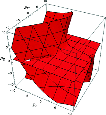
Singular locus about variables of position. Whether Rodriguez parameters or quaternion can be used to describe the rotation matrix. The singular locus is identical.
-
(2)
When the variables of position of the moving platform are determined, the change of the singular locus with respect to orientation variables can be researched by Eq. (17) or Eq. (18). For example, the position vector is defined as \( \varvec{P} = \left( {\begin{array}{*{20}c} 2 & 2 & 4 \\ \end{array} } \right)^{T} \), the rotation matrix is described by Rodriguez parameters; The singular locus equations is 6 times polynomial about of Rodriguez parameters \( U \), \( V \), \( W \), singular locus is shown in Fig. 3. When the rotation matrix is described by quaternion; The singular locus equations is 8 times polynomial about that of each component of quaternion (\( \varepsilon_{0} = \sqrt {1 - \varepsilon_{1}^{2} - \varepsilon_{2}^{2} - \varepsilon_{3}^{2} } \)) singular locus is shown in Fig. 4.
Fig. 3. 
Singular locus about variables of orientation at the given position. The variables of orientation are described by Rodriguez parameters.
Fig. 4. 
Singular locus about variables of orientation at the given position. The variables of orientation are described by quaternions.
-
(3)
When the variables of position and orientation of the moving platform are determined, whether Stewart platform parallel mechanism is singular or not can be researched by Eq. (17) or Eq. (18). For example, the position vector is defined as \( \varvec{P} = \left( {\begin{array}{*{20}c} 0 & 0 & 5 \\ \end{array} } \right)^{T} \); Rodriguez parameters are U = 0, V = 0 and W = 1 respectively; singular locus equation is equal to zero, Stewart platform parallel mechanism occurs singular.


6 Conclusions
-
(1)
In this paper, a new approach used to analyze the singularity of the Stewart Platform parallel mechanism is studied. There are only 258 items in analytical expression of the singular locus equation when it is expanded completely.
-
(2)
The rotation matrix is described by quaternion, and the kinematics equation of the Stewart Platform parallel mechanism is transformed into a new form in this paper. In addition, normalization of quaternion is used and 7 equivalent equations are obtained, which can be used to study the singularity and the forward kinematics of the Stewart Platform parallel mechanism.
-
(3)
Based on these equivalent equations, this paper presents a new Jacobian matrix, which states the mapping relationship between the driving speed and the change rate of position and orientation of the moving platform. Every component of the Jacobian matrix is a rather simple monomial.
-
(4)
Evaluating the determinant of Jacobian matrix, the analytical expression of the singular locus equation can be derived. These singular trajectory equations can not only be used to study the distribution of singular locus in the workspace, but can also be used to judge whether a set of parameters of position and orientation corresponds to a singularity pose. The singularity analysis approach presented in this paper provides an important theoretical basis for studying the singularity free workspace.
References
Merlet, J.P.: Parallel Robots. Springer, Netherlands (2006)
Tsai, L.W.: Robot Analysis: The Mechanics of Serial and Parallel Manipulators. Wiley, New York (1999)
Cheng, S.L., Wu, H.T., Wang, C.Q., et al.: A novel method for singularity analysis of the 6-SPS parallel mechanisms. Sci. China Technol. Sci. 54(5), 1220–1227 (2011)
Gosselin, C.M., Angeles, J.: Singularity analysis of closed-loop kinematic chains. IEEE Trans. Robot. Autom. 6(3), 281–290 (1990)
Mayer St-Onge, B., Gosselin, C.M.: Singularity analysis and representation of the general Gough-Stewart platform. Int. J. Robot. Res. 19(3), 271–288 (2000)
Jiang, Q.M., Gosselin, C.M.: Determination of the maximal singularity-free orientation workspace for the Gough-Stewart platform. Mech. Mach. Theory 44(6), 1281–1293 (2009)
Huang, Z., Cao, Y.: Property identification of the singularity loci of a class of the Gough-Stewart manipulators. Int. J. Robot. Res. 24(8), 675–685 (2005)
Huang, Z., Zhao, Y.Z., Zhao, T.S.: Advanced spatial mechanism. Higher Education Press, Beijing (2014)
Coste, M., Moussa, S.: On the rationality of the singularity locus of a Gough-Stewart platform - Biplanar case. Mech. Mach. Theory 80, 82–92 (2015)
Karimi, A., Masouleh, M.T., Cardou, P.: Singularity-free workspace analysis of general 6-UPS parallel mechanisms via convex optimization. Mech. Mach. Theory 80, 17–34 (2014)
Cao, Y., Wu, M.P., Zhou, H.: Position-singularity characterization of a special class of the Stewart parallel mechanisms. Int. J. Robot. Autom. 28(1), 57–64 (2013)
Hunt, K.H.: Kinematic Geometry of Mechanisms. The Clarendon Press, Oxford University Press, New York (1978)
Huang, Z., Zhao, Y., Wang, J., et al.: Kinematic principle and geometrical condition of general-linear-complex special configuration of parallel manipulators. Mech. Mach. Theory 34(8), 1171–1186 (1999)
Merlet, J.P.: Singular configurations of parallel manipulators and Grassmann geometry. Int. J. Robot. Res. 8(5), 45–56 (1989)
Caro, S., Moroz, G., Gayral, T., et al.: Singularity analysis of a six-dof parallel manipulator using grassmann-cayley algebra and gröbner bases. In: Angeles, J., Boulet, B., Clark, J.J., Kövecses, J., Siddiqi, K. (eds.) Proceedings of an International Symposium on the Occasion of the 25th Anniversary of the McGill University Centre for Intelligent Machines 2010, pp. 341–352. Springer, Berlin Heidelberg (2010)
Doyon, K., Gosselin, C., Cardou, P.: A vector expression of the constant-orientation singularity locus of the Gough-Stewart platform. ASME J. Mech. Robot. 5(3), 1885–1886 (2013)
Liu, G.J., Qu, Z.Y., Liu, X.C., et al.: Singularity analysis and detection of 6-UCU parallel manipulator. Robot. Comput.-Integr. Manuf. 30(2), 172–179 (2014)
Shanker, V., Bandyopadhyay, S.: Singular manifold of the general hexagonal stewart platform manipulator. In: Lenarcic, J., Husty, M. (eds.) Latest Advances in Robot Kinematics 2012, pp. 397–404. Springer, Dordrecht (2012)
Kaloorazi, M.H.F., Masouleh, M.T., Caro, S.: Interval-analysis-based determination of the singularity-free workspace of Gough-Stewart parallel robots. In: Iranian Conference on Electrical Engineering 2013, IEEE, pp. 1–6. IEEE, Mashhad (2013)
Gosselin, C.M., Schreiber, L.-T.: Kinematically Redundant Spatial Parallel Mechanisms for Singularity Avoidance and Large Orientational Workspace. IEEE Trans. Robot. 32(2), 286–300 (2016)
Agarwal, A., Nasa, C., Bandyopadhyay, S.: Dynamic singularity avoidance for parallel manipulators using a task-priority based control scheme. Mech. Mach. Theory 96, 107–126 (2016)
Parsa, S.S., Boudreau, R., Carretero, J.A.: Reconfigurable mass parameters to cross direct kinematic singularities in parallel manipulators. Mecha. Mach. Theory 85, 53–63 (2015)
Pagis, G., Bouton, N., Briot, S., et al.: Enlarging parallel robot workspace through Type-2 singularity crossing. Control Eng. Pract. 39, 1–11 (2015)
Aminea, S., Masoulehb, M.T., Caro, S., et al.: Singularity analysis of 3T2R parallel mechanisms using Grassmann-Cayley algebra and Grassmann geometry. Mech. Mach. Theory 52, 326–340 (2012)
Kim, J.S., Jin, H.J., Park, J.H.: Inverse kinematics and geometric singularity analysis of a 3-SPS/S redundant motion mechanism using conformal geometric algebra. Mech. Mach. Theory 90, 23–36 (2015)
Chai, X.X., Xiang, J.N., Li, Q.C.: Singularity analysis of a 2-UPR-RPU parallel mechanism. J. Mech. Eng. 51(13), 144–151 (2015)
Kuipers, J.B.: Quaternions and Rotation Sequences: A Primer with Applications to Orbits. Aerospace and Virtual Reality. Princeton University Press, Princeton (1999)
Acknowledgment
The authors gratefully acknowledge the supported of the National Natural Science Foundation of China (Grant No. 51405417), the supported of Natural Science Foundation of Jiangsu Province, China (Grant No. BK20140470).
Author information
Authors and Affiliations
Corresponding author
Editor information
Editors and Affiliations
Rights and permissions
Copyright information
© 2017 Springer International Publishing AG
About this paper
Cite this paper
Cheng, S., Su, G., Xiong, X., Wu, H. (2017). A Singularity Analysis Method for Stewart Parallel Mechanism with Planar Platforms. In: Huang, Y., Wu, H., Liu, H., Yin, Z. (eds) Intelligent Robotics and Applications. ICIRA 2017. Lecture Notes in Computer Science(), vol 10463. Springer, Cham. https://doi.org/10.1007/978-3-319-65292-4_38
Download citation
DOI: https://doi.org/10.1007/978-3-319-65292-4_38
Published:
Publisher Name: Springer, Cham
Print ISBN: 978-3-319-65291-7
Online ISBN: 978-3-319-65292-4
eBook Packages: Computer ScienceComputer Science (R0)