Symbolic Verification and Strategy Synthesis for Linearly-Priced Probabilistic Timed Automata

Abstract

Probabilistic timed automata are a formalism for modelling systems whose dynamics includes probabilistic, nondeterministic and timed aspects including real-time systems. A variety of techniques have been proposed for the analysis of this formalism and successfully employed to analyse, for example, wireless communication protocols and computer security systems. Augmenting the model with prices (or, equivalently, costs or rewards) provides a means to verify more complex quantitative properties, such as the expected energy usage of a device or the expected number of messages sent during a protocol’s execution. However, the analysis of these properties on probabilistic timed automata currently relies on a technique based on integer discretisation of real-valued clocks, which can be expensive in some cases. In this paper, we propose symbolic techniques for verification and optimal strategy synthesis for priced probabilistic timed automata which avoid this discretisation. We build upon recent work for the special case of expected time properties, using value iteration over a zone-based abstraction of the model.

These keywords were added by machine and not by the authors. This process is experimental and the keywords may be updated as the learning algorithm improves.

1 Introduction

Real-time systems are at the heart of application domains such as communication protocols, embedded systems, hardware circuits, autonomous transport, robotics and manufacturing. The presence of hard real-time constraints within a distributed, reactive environment means that their correct functioning depends on the timing pattern of the interaction of the system with its environment, making correctness guarantees difficult.

Timed automata [2] are a powerful formalism for modelling and verification of real-time systems. They are finite-state automata equipped with real-valued clocks which measure the passage of time, and whose transitions are annotated with guards that specify the time constraints that have to be satisfied for the transition to be taken. Since timed automata allow the modelling of dense real-time, the decidability of model checking depends on a number of assumptions.

Several verification approaches have been introduced, see e.g. [1, 21, 22, 32], of which the symbolic zone-based approach enables greater scalability compared to the digital clocks method, which assumes an integral model of time as opposed to a dense model of time. Timed automata have been widely used for modelling and analysis of real-world systems; in particular, they are supported by the UPPAAL [31] model checker, the gold standard in computer-aided verification for real-time systems.

When modelling and analysing real-time systems, it is often necessary to consider quantities other than time, for example energy consumption, network bandwidth or number of packets lost. The model of (linearly) priced timed automata [3, 7] extends timed automata with prices (weights) annotating the locations and transitions, thus enabling reasoning about costs or rewards accumulated over time as the execution progresses. This model has good decidability properties and several algorithms have been proposed for its analysis, based on an extension of regions or zones with prices. Priced timed automata are also supported by UPPAAL, and have been used for timing analysis of a range of embedded real-time systems, with several flaws discovered and corrected.

However, many distributed real-time systems also employ randomisation, for example random back-off in wireless network protocols. A natural model for such systems is a probabilistic extension of (priced) timed automata called probabilistic timed automata (PTAs) [6, 19, 29]. They can be viewed as timed automata whose transitions are probability distributions over the set of edges, where each such edge specifies a successor location and a set of clocks to reset.

A key property studied here is expected reachability, namely the expected time/price until some event occurs. This problem has been found unsuitable for symbolic zone-based methods, including priced zones, since accumulated prices are unbounded. Recently, [24, 25] introduced a zone-based symbolic method to compute minimum and maximum expected time for PTAs and to synthesise a corresponding strategy. Prior to this, expected reachability properties of PTAs could only be verified using the digital clocks method [28] that can suffer from state-space explosion.

Probabilistic timed automata are supported by the PRISM [27] model checker via the zone-based and digital clocks abstractions (though not yet the method of [25]) and have used been for the analysis of a broad range of real-world protocols, see for example [18, 28]. A second tool supporting PTAs is mcpta [20], which applies the digital clocks abstraction to translate a subset of the modelling language Modest [15] directly into the PRISM modelling language. The related problem of price-bounded probabilistic reachability [10] (known to be undecidable [9]) can be analysed via a semi-decision procedure using priced zones, implemented in Fortuna [11].

In this paper we study the computation of the minimum/maximum expected price for linearly-priced probabilistic timed automata, for which, to the best of our knowledge, no zone-based method exists at present. More specifically, we extend [25], where only the restricted case of expected time is considered. The minimum expected price problem for a related model of priced timed games in stochastic environments was tackled in [16] using statistical model checking with Uppaal-SMC. Since this approach is based on simulation, rather than numerical model checking, it gives approximate results with probabilistic guarantees.

As in [24, 25], our method relies on an interpretation of the PTA as an uncountable-state Markov decision process (MDP) and employs a representation in terms of an extension of the ‘simple’ and ‘nice’ functions of [4]. The optimal prices are computed via a Bellman equation using value iteration, which gives guaranteed eventual convergence to the correct values. Moreover, an $\varepsilon$-optimal strategy can be extracted by stepping backwards and retrieving the locally optimal choices once some convergence criterion has been satisfied. For minimum expected time, it is always optimal to let as little time pass as possible. However, for minimum price, it turns out that this is not always the case, and it can be optimal to let time pass now and accumulate a lower price, as opposed to waiting and accumulating a higher price later. The case of maximum time/price is dual.

Paper Structure. In Sect. 2 we summarise the relevant background, mainly concerning uncountable MDPs and the computation of optimal reward. Section 3 defines the priced extension of probabilistic timed automata (PTAs) and their interpretation as an uncountable MDP under appropriate assumptions. In Sect. 4, we introduce a representation of the value functions that generalise the simple and nice functions of [4], and present our algorithms for computing optimal expected price and synthesis of an $\varepsilon$-optimal strategy using the backwards zone graph of a PTA.

2 Background

Let $\mathbb {R}$ denote the non-negative reals, $\mathbb {N}$ natural numbers, $\mathbb {Q}$ rationals and $\mathbb {Q}_{+}$ non-negative rationals. A discrete probability distribution over a (possibly uncountable) set S is a function $\mu : S {\rightarrow } [0,1]$ such that $\sum _{s\in S}\mu (s)=1$ and the set $\{ s \in S \;|\;\mu (s){>}0 \}$ is finite. Let $\mathsf {dist}(S)$ denote the set of distributions over S. A distribution $\mu \in \mathsf {dist}(S)$ is a point distribution if $\mu (s)=1$ for some $s \in S$.

In preparation for the sections that follow, we present some background material and known results for the model of Markov decision processes (MDPs).

Definition 1

An MDP is a tuple $\mathsf {M}=(S,s_0,A, Prob _\mathsf {M}, Price _\mathsf {M})$, where:

• S is a (possibly uncountable) set of states and $s_0\in S$ is an initial state;

• A is a (possibly uncountable) set of actions;

• $Prob _\mathsf {M}: S \times A \rightarrow \mathsf {dist}(S)$ is a (partial) probabilistic transition function;

• $Price _\mathsf {M}: S \times A \rightarrow \mathbb {R}$ is a price function.

In each state s of an MDP $\mathsf {M}$, there is a set of enabled actions, denoted by A(s), containing those actions a for which $Prob _\mathsf {M}(s,a)$ is defined. In state s, a transition corresponds to first nondeterministically choosing an available action and, assuming action $a\in A(s)$ is chosen, then selecting a successor state randomly according to the distribution $Prob _\mathsf {M}(s,a)$. Taking an a-labelled transition from state s incurs a price of $Price _\mathsf {M}(s,a)$. We use the terminology “price” for consistency with the model of priced probabilistic timed automata used later, but these are commonly also referred to as costs or, dually, rewards for MDPs.

A path of an MDP $\mathsf {M}$ is given by a finite or infinite sequence of transitions $\omega =s_0{\xrightarrow {a_0}}s_1{\xrightarrow {a_1}}s_2{\xrightarrow {a_2}} {\cdots }$ with $Prob _\mathsf {M}(s_i,a_i)(s_{i+1})>0$ for all $i \ge 0$. The $(i+1)$th state of a path $\omega$ and action associated with the $(i+1)$th transition are denoted by $\omega (i)$ and $\omega [i]$ respectively. The set of infinite (finite) paths is denoted by $IPaths _{\mathsf {M}}$ ($FPaths _{\mathsf {M}}$) and the last state of a finite path $\omega$ by $last (\omega )$.

A strategy (also called an adversary, scheduler or policy) of an MDP $\mathsf {M}$ represents one resolution of the nondeterminism in $\mathsf {M}$.

Definition 2

A strategy of an MDP $\mathsf {M}$ is a function $\sigma : FPaths _\mathsf {M}{\rightarrow } \mathsf {dist}(A)$ such that $\sigma (\omega )(a){>}0$ only if $a \in A( last (\omega ))$.

For a given strategy $\sigma$ and state s of an MDP $\mathsf {M}$, we can construct a probability measure $\mathcal {P}_s^\sigma$ over the set of infinite paths starting in s [26]. A strategy $\sigma$ is memoryless if its choices only depend on the current state, and deterministic if $\sigma (\omega )$ is a point distribution for all $\omega \in FPaths _\mathsf {M}$. The set of all strategies of MDP $\mathsf {M}$ is denoted $\varSigma _{\mathsf {M}}$.

Key quantitative properties for MDPs are the probability of reaching a target and the expected price incurred before doing so. We will refer to these as probabilistic reachability and expected reachability, respectively. For a strategy $\sigma$, state s and set of target states $F\subseteq S$ of an MDP $\mathsf {M}$, these values are given by:

where for any infinite path $\omega$:

and $k_F = \min \{ k-1 \;|\;\omega (k) \in F\}$ if there exists $k \in \mathbb {N}$ such that $\omega (k) \in F$ and $k_F = \infty$ otherwise. As usual we consider the optimal values of these properties, i.e. the minimum and maximum values over all strategies:

One approach to computing these optimal values is through Bellman operators [8] using either value iteration or policy iteration [12, 13]. In the case of expected reachability, the Bellman operators have the following form.

Definition 3

Let $\mathsf {M}$ be an MDP with state space $S, F \subseteq S$ be a target set, and let $\mathrm {opt}\in \{\min ,\max \}$. The Bellman operator $T^{\mathrm {opt}}_\mathsf {M}: (S {\rightarrow } \mathbb {R}) \rightarrow (S {\rightarrow } \mathbb {R})$ for optimal expected reachability is defined as follows. For any function $f : S \rightarrow \mathbb {R}$ and state $s \in S$:

$$\begin{aligned} \begin{array}{c} T^{\mathrm {opt}}_\mathsf {M}(f)(s) = {\left\{ \begin{array}{ll} 0 &{} \textit{if}\,\, s \in F \\ \mathrm {opt}^\star _{\!\!a \in A(s)} \left\{ Price _\mathsf {M}(s,a) + \sum \nolimits _{s'\in S} Prob _\mathsf {M}(s,a)(s') \cdot f(s') \right\} \!\!\!\! &{} \textit{if}\,\, s \not \in F \end{array}\right. } \end{array} \end{aligned}$$

where $\min ^\star = \inf$ and $\max ^\star = \sup$.

Value iteration works by starting with an initial approximation $f_0:S\rightarrow \mathbb {R}$ and repeatedly applying $T^{\mathrm {opt}}_\mathsf {M}$ until it converges to the optimal expected reachability value. In practice, an approximate result is obtained by terminating the computation once some convergence criterion is satisfied, for example, by checking that the maximum pointwise difference between $(T^{\mathrm {opt}}_\mathsf {M})^{n}(f_0)$ and $(T^{\mathrm {opt}}_\mathsf {M})^{n+1}(f_0)$ is below some threshold $\varepsilon \in \mathbb {R}$. The process also yields an (approximately) optimal strategy for either minimising or maximising expected reachability. Policy iteration starts from a (deterministic and memoryless) strategy, and repeatedly attempts to find an improved (deterministic and memoryless) strategy by computing the expected reachability values for the current strategy and trying to update action choices to optimise expected reachability values.

Below, we state some known results from [23] regarding MDPs and value iteration, which are needed later in the paper (and which were adapted for the case of PTAs in [25]). This requires us to make the following assumptions.

Assumption 1

For any MDP $\mathsf {M}=(S,s_0,A, Prob _\mathsf {M}, Price _\mathsf {M})$ and target set F:

• (a) A(s) is compact for all $s \in S$;

• (b) $Price _\mathsf {M}$ is bounded and $a \mapsto Price _\mathsf {M}(s,a)$ is continuous for all $s \in S$;

• (c) if $\sigma$ is a memoryless, deterministic strategy which is not proper, then $\mathbb {E}_\mathsf {M}^\sigma (s,F)$ is unbounded for some $s \in S$;

• (d) there exists a proper, memoryless, deterministic strategy;

where a strategy $\sigma$ is called proper if $\mathbb {P}^{\sigma }_{\mathsf {M}}(s,F)=1$ for all $s \in S$.

Theorem 1

[23]. If $\mathsf {M}$ and F are an MDP and target set for which Assumption 1 holds, and the minimum expected price values are bounded below, then:

• there exists a memoryless, deterministic strategy that achieves the minimum expected price of reaching F;

• the minimum expected price values are the unique solutions to $T^{\min }_\mathsf {M}$;

• value iteration over $T^{\min }_\mathsf {M}$ converges to the minimum expected price values when starting from any bounded function;

• policy iteration converges to the minimum expected price values when starting from any proper, memoryless, deterministic strategy.

Corollary 1

If $\mathsf {M}$ and F are an MDP and target set for which Assumption 1 holds and the maximum expected price values are bounded above, then:

• there exists a memoryless, deterministic strategy that achieves the maximum expected price of reaching F;

• the maximum expected price values are the unique solutions to $T^{\max }_\mathsf {M}$;

• value iteration over $T^{\max }_\mathsf {M}$ converges to the maximum expected price values when starting from any bounded function;

• policy iteration converges to the maximum expected price values when starting from any proper, memoryless, deterministic strategy.

3 Priced Probabilistic Timed Automata

In this section we introduce probabilistic timed automata (PTAs) [6, 19, 29], a formalism for modelling systems whose dynamics includes probabilistic, nondeterministic and timed aspects, and the extended model of linearly-priced PTAs [28], which augment PTAs with prices. We will commonly refer to the latter simply as PTAs.

Clocks, Clock Valuations and Zones. We assume we have a finite set $\mathcal {X}$ of real-valued variables called clocks which increase at the same, constant rate. A clock valuation is a function $v: \mathcal {X}{\rightarrow } \mathbb {R}$ and let $\mathbb {R}^\mathcal {X}$ be the set of all clock valuations. We denote by $\mathbf {0}$ the clock valuation that assigns 0 to all clocks. For any subset of clocks R, non-negative real value t and clock valuation v, v[R] is the clock valuation where $v[R](x)=0$ if $x\in R$ and $v[R](x)=v(x)$ if $x \in \mathcal {X}{\setminus } R$, and $v+t$ is the clock valuation where $(v+t)(x)=v(x)+t$ for all $x\in \mathcal {X}$. The set of zones over $\mathcal {X}$, written $Zones (\mathcal {X})$, is defined by the syntax:

$$\begin{aligned} \zeta \mathrel {\mathop :}\mathrel {\mathop :}=\mathtt {true} \;|\;x \le d \;|\;c \le x \;|\;x+c \le y+d \;|\;\lnot \zeta \;|\;\zeta \wedge \zeta \end{aligned}$$

where $x,y \in \mathcal {X}$ and $c,d \in \mathbb {N}$. We can restrict the syntax to convex zones by removing negation. For a clock valuation v and zone $\zeta$, we say v satisfies $\zeta$, denoted $v {\models } \zeta$, if $\zeta$ is true after substituting each occurrence of each clock x with v(x). The semantics of a zone $\zeta$ is the set of clock valuations satisfying it. We require the following zone operations [33], for zone $\zeta$ and subset of clocks R:

• $\swarrow \!\!\zeta = \{ v \in \mathbb {R}^\mathcal {X}\;|\;\exists t \in \mathbb {R}. \, v+t \models \zeta \}$;

• $\zeta [R] = \{ v[R] \;|\;v \models \zeta \}$;

• $[R]\zeta = \{ v \in \mathbb {R}^\mathcal {X}\;|\;v[R] \models \zeta \}$.

Syntax and Semantics of PTAs. We now present the formal syntax and semantics of linearly-priced PTAs.

Definition 4

A linearly-priced probabilistic timed automaton (PTA) $\mathsf {P}$ is a tuple $(L,l_0,\mathcal {X}, Act , \mathsf {enab}, \mathsf {prob}, \mathsf {inv},\mathsf {price})$ where:

• L is a finite set of locations and $l_0 \in L$ is an initial location;

• $\mathcal {X}$ is a finite set of clocks;

• $Act$ is a finite set of actions;

• $\mathsf {enab}: L \times Act \rightarrow Zones (\mathcal {X})$ is an enabling condition;

• $\mathsf {prob}: L \times Act \rightarrow \mathsf {dist}(2^\mathcal {X}\times L)$ is a probabilistic transition function;

• $\mathsf {inv}: L\rightarrow Zones (\mathcal {X})$ is an invariant condition;

• $\mathsf {price}= (\mathsf {price}_{L},\mathsf {price}_{ Act })$ is a price structure where $\mathsf {price}_{L}: L \rightarrow \mathbb {Q}_{+}$ is a location price function and $\mathsf {price}_{ Act }: L \times Act \rightarrow \mathbb {Q}_{+}$ an action price function.

The underlying semantics of PTA $\mathsf {P}$ is an MDP with an infinite set of both states and actions. The states are location-valuation pairs (l, v) such that v satisfies the invariant $\mathsf {inv}(l)$ and the initial state is the initial location with all clocks set to 0. The available actions in state (l, v) are the time-action pairs (t, a) such the invariant $\mathsf {inv}(l)$ remains true while letting t time units pass, after this time the enabling condition $\mathsf {enab}(l,a)$ is satisfied, and the successor location and the clocks that are reset are then chosen according to the distribution $\mathsf {prob}(l,v)$. Furthermore, a price is incurred at rate $\mathsf {price}_{L}(l)$ while letting the t time units pass and a price $\mathsf {price}_{ Act }(l,a)$ is incurred when performing the action a.

Definition 5

For a PTA $\mathsf {P}=(L,l_0,\mathcal {X}, Act , \mathsf {enab}, \mathsf {prob}, \mathsf {inv},\mathsf {price})$ the semantics of $\mathsf {P}$ is given by the MDP $[ \! [ {\mathsf {P}} ] \! ]=(S,s_0, \mathbb {R}\times Act , Prob _{ [ \! [ {\mathsf {P}} ] \! ]}, Price _{ [ \! [ {\mathsf {P}} ] \! ]})$ where:

• $S=\{(l,v)\in L \times \mathbb {R}^{\mathcal {X}} \;|\;v \models \mathsf {inv}(l)\}$ and $s_0= (l_0,\mathbf {0})$;

• if $(l,v) \in S$ and $(t,a) \in \mathbb {R}\times Act$, then $Prob _{ [ \! [ {\mathsf {P}} ] \! ]}((l,v),(t,a))=\mu$ if and only if $v+t' \models \mathsf {inv}(l)$ for $0 \le t' \le t$, $v+t \models \mathsf {enab}(l,a)$ and for any $(l',v')\in S$:

  $$\begin{aligned} \begin{array}{c} \mu (l',v')= \sum \nolimits _{R \subseteq \mathcal {X}\wedge v'=(v+t)[R]} \mathsf {prob}(l,a)(R,l') \end{array} \end{aligned}$$

• $Price _{ [ \! [ {\mathsf {P}} ] \! ]}((l,v),(t,a)) = \mathsf {price}_{L}(l) \cdot t + \mathsf {price}_{ Act }(l,a)$ for all $(l,v) \in S$ and $(t,a) \in \mathbb {R}\times Act$.

Expected Prices. The property of PTAs on which we focus in this paper is the optimal (minimum or maximum) expected price incurred before reaching a target, which is defined along the same lines as the equivalent property for MDPs defined in Sect. 2. The differences are that, firstly, the target is now defined as a set $F\subseteq L$ of locations and, secondly, prices are incurred both when time elapses in a location, and when an action is performed. Since the semantics of a PTA is an (infinite-state) MDP, the expected price for a PTA is defined in straightforward fashion in terms of the MDP. For PTA $\mathsf {P}$, target locations F, state (l, v) and $\mathrm {opt}\in \{\min ,\max \}$, we have:

When computing these values, we make several assumptions about PTAs, similar to those imposed in [25]. Firstly, this will ensure that Assumption 1 holds for the underlying MDP, which allows us to apply Theorem 1 and Corollary 1. Secondly, it makes sure that unrealistic behaviours are discarded.

Assumption 2

For any PTA $\mathsf {P}$, we have:

• (a) all invariants of $\mathsf {P}\!$ are bounded;

• (b) only non-strict inequalities are allowed in clock constraints, i.e., $\mathsf {P}\!$ is closed;

• (c) all invariant and enabling conditions of $\mathsf {P}\!$ are convex;

• (d) all location prices of $\mathsf {P}\!$ are positive;

• (e) $\mathsf {P}\!$ is structurally non-zeno [34] (this can be identified syntactically and in a compositional fashion [35] and guarantees time-divergent behaviour).

The reasons for these assumptions are similar to those given in [25]. The main difference is that, in order to ensure that Assumption 1(c) holds, we require that all location prices are positive (Assumption 2(d)), in addition to the structural non-zeno assumption. More precisely, for any PTA satisfying Assumption 2(d) and (e), if, from some state and under some strategy a target is not reached with probability 1, then from this state and under this strategy the expected price of reaching the target is infinite. Expected time (as in [25]) is a special case of expected price where all action prices are 0 and all location prices are 1, and therefore Assumption 1(d) will always hold in this case.

4 Optimal Expected Price Algorithms for PTAs

In this section, we present our symbolic approach for computing optimal expected reachability prices and for synthesising a corresponding optimal strategy. We first extend the approach of [25] for computing optimal expected times, a key building block of which is an initial backwards exploration of the state space, using the techniques from [30]. Computing expected rewards can then be performed using value iteration over the zone graph constructed during backwards exploration. This process is described in Sect. 4.1. Next, in Sect. 4.2, we discuss the use of rational k-simple functions and rational (r, k)-nice functions to represent the prices stored during value iteration. Finally, Sect. 4.3 presents an example of the process.

To simplify the presentation, for the remainder of this section we will fix a PTA $\mathsf {P}=(L,l_0,\mathcal {X}, Act , \mathsf {enab}, \mathsf {prob}, \mathsf {inv},\mathsf {price})$, target set of locations $F\subseteq L$ and let $[ \! [ {\mathsf {P}} ] \! ]=(S,s_0, \mathbb {R}\times Act , Prob _{ [ \! [ {\mathsf {P}} ] \! ]}, Price _{ [ \! [ {\mathsf {P}} ] \! ]})$.

4.1 Computation of Expected Prices and Optimal Strategies

The first step is the construction of a zone graph ${\mathtt {G}}=({\mathtt {Z}},{\mathtt {E}})$, whose vertices ${\mathtt {Z}}$ are symbolic states. A symbolic state of $\mathsf {P}$ is a location-zone pair $(l, \zeta )$ and represents the set of states $\{ (l,v) \;|\;v \in \mathbb {R}^\mathcal {X}\wedge v \models \zeta {\wedge } \mathsf {inv}(l) \}$ of $[ \! [ {\mathsf {P}} ] \! ]$. If ${\mathtt {z}}=(l,\zeta )$ and ${\mathtt {z}}' = (l,\zeta ')$ are symbolic states, then let ${\mathtt {z}}{\wedge } {\mathtt {z}}' = (l, \zeta {\wedge } \zeta '), {\mathtt {z}}\subseteq {\mathtt {z}}'$ when $\zeta \subseteq \zeta '$ and ${\mathtt {z}}=\varnothing$ if and only if $\zeta = \mathtt {false}$. For any symbolic state ${\mathtt {z}}=(l,\zeta )$, locations $l'$ and $l''$, action a and set of clocks R we will use the following time and discrete predecessor operations:

As in [25], we use the backwards reachability algorithm of [30] (adding action labels to the edge tuples) to build a zone graph, shown in Fig. 1.

Fig. 1.

Backwards reachability algorithm [30]

Given a zone graph ${\mathtt {G}}=({\mathtt {Z}},{\mathtt {E}})$, for any $(l,\zeta ) \in {\mathtt {Z}}$ let ${\mathtt {E}}(l,\zeta ) \subseteq 2^{{\mathtt {E}}}$ represent the following sets of edges: $E \in {\mathtt {E}}(l,\zeta )$ if and only if there exists $a \in Act$ such that $\mathsf {edges}(l,a) = \{ (R_1,l_1),\dots ,(R_n,l_n)\}$ and:

$$\begin{aligned} E=\{ ({\mathtt {z}},a,(R_1,l_1),{\mathtt {z}}_1) , \dots , ({\mathtt {z}},a,(R_n,l_n),{\mathtt {z}}_n) \} \end{aligned}$$

for some ${\mathtt {z}}_1,\dots ,{\mathtt {z}}_n \in {\mathtt {Z}}$.

After building the zone graph, the next step is to find and restrict $[ \! [ {\mathsf {P}} ] \! ]$ and ${\mathtt {G}}$ to include only those states for which the optimal expected price to reach the target is finite, i.e., states for which the maximum probability of reaching the target is 1 in the case of minimum expected prices and for which the minimum probability of reaching the target is 1 in the case of maximum expected prices.

Symbolic (zone-based) algorithms for performing this restriction, which extend the algorithms developed for MDPs [14, 17], can be found in [25]. For the remainder of the section we suppose that $S_{\min }$ and $S_{\max }$ are the states of $[ \! [ {\mathsf {P}} ] \! ]$ for which the minimum and maximum reachability probability is 1, and $[ \! [ {\mathsf {P}} ] \! ]_{\min }$ and $[ \! [ {\mathsf {P}} ] \! ]_{\max }$ are the sub-MDPs restricted to these sets of states. We will also assume that ${\mathtt {G}}_{\min } = ({\mathtt {Z}}_{\min },{\mathtt {E}}_{\min })$ and ${\mathtt {G}}_{\max } = ({\mathtt {Z}}_{\max },{\mathtt {E}}_{\max })$ are the restrictions of the zone graph ${\mathtt {G}}=({\mathtt {Z}},{\mathtt {E}})$ to these sets of states.

It follows that the restricted MDPs $[ \! [ {\mathsf {P}} ] \! ]_{\min }$ and $[ \! [ {\mathsf {P}} ] \! ]_{\max }$ satisfy Assumption 1, and we can therefore use Theorem 1 in the case of minimum expected pices and Corollary 1 in the case of maximum expected prices. In particular, we can use the fact that value iteration for the Bellman operators $T^{\min }_{ [ \! [ {\mathsf {P}} ] \! ]_{\min }}$ and $T^{\max }_{ [ \! [ {\mathsf {P}} ] \! ]_{\max }}$ (see Definition 3) for the target set $S_F$ converges to the minimum and maximum expected prices, respectively, when starting from any bounded function.

Next, we present a value iteration method over the restricted zone graphs ${\mathtt {G}}_{\min }$ and ${\mathtt {G}}_{\max }$, based on the function $T^{\mathrm {opt}}_{{\mathtt {G}}_{\mathrm {opt}}}$, which has a direct correspondence with value iteration over the sub-MDPs $[ \! [ {\mathsf {P}} ] \! ]_{\min }$ and $[ \! [ {\mathsf {P}} ] \! ]_{\max }$.

Definition 6

The operator $T^{\mathrm {opt}}_{{\mathtt {G}}_{\mathrm {opt}}} : ({\mathtt {Z}}_{\mathrm {opt}} {\rightarrow } (S_{\mathrm {opt}} {\rightarrow } \mathbb {R})) {\rightarrow } ({\mathtt {Z}}_{\mathrm {opt}} {\rightarrow } (S_{\mathrm {opt}} {\rightarrow } \mathbb {R}))$ on the zone graph ${\mathtt {G}}_{\mathrm {opt}}$ is such that for $g : {\mathtt {Z}}_{\mathrm {opt}} {\rightarrow } (S_{\mathrm {opt}} {\rightarrow } \mathbb {R}), {\mathtt {z}}=(l,\zeta ) \in {\mathtt {Z}}_{\mathrm {opt}}$ and $s=(l,v) \in S_{\mathrm {opt}}$ where $s \in \mathsf {tpre}({\mathtt {z}})$ we have $T^{\mathrm {opt}}_{{\mathtt {G}}_{\mathrm {opt}}}(g)({\mathtt {z}})(s)$ equals 0 if $l \in F$ and otherwise equals:

for $\mathrm {opt}\in \{ \min , \max \}$, and where $\min ^\star = \inf$ and $\max ^\star = \sup$.

The proof of the following proposition follows directly from the proofs presented in [25] for optimal expected time computation.

Proposition 1

For $\mathrm {opt}\in \{ \min , \max \}$, if $f : S_{\mathrm {opt}} {\rightarrow } \mathbb {R}$ and $g : {\mathtt {Z}}_{\mathrm {opt}} {\rightarrow } (S_{\mathrm {opt}} {\rightarrow } \mathbb {R})$ are functions such that $f(s) = g({\mathtt {z}})(s)$ for all $s \in S_{\mathrm {opt}}$ and ${\mathtt {z}}\in {\mathtt {Z}}_{\mathrm {opt}}$ such that $s \in \mathsf {tpre}({\mathtt {z}})$, then for any $s \in S_{\mathrm {opt}}$ and $n \in \mathbb {N}$ we have:

$$\begin{aligned} (T^{\mathrm {opt}}_{ [ \! [ {\mathsf {P}} ] \! ]_{\mathrm {opt}}})^n(f)(s) = \mathrm {opt}\{ \, (T^{\mathrm {opt}}_{{\mathtt {G}}_{\mathrm {opt}}})^n(g)({\mathtt {z}})(s) \;|\;{\mathtt {z}}\in {\mathtt {Z}}_{\mathrm {opt}} \wedge s \in \mathsf {tpre}({\mathtt {z}}) \, \}. \end{aligned}$$

Consequently, value iteration, using function $T^{\mathrm {opt}}_{{\mathtt {G}}_{\mathrm {opt}}}$, converges to the optimal expected reachability price for the original PTA, a result that follows from Theorem 1, Corollary 1 and Proposition 1. The final step is then to synthesise an $\varepsilon$-optimal deterministic, memoryless strategy for expected reachability on the PTA. This can be done by stepping through the backwards graph and selecting the time-action pairs that achieve the results returned by value iteration in each state of the zone graph.

Unlike traditional value iteration for MDPs, which iterates over real-valued vectors over states, the value iteration process for PTAs outlined above uses state vectors whose values are themselves real-valued functions. In the following section, we will show how this can be achieved using classes of functions called rational k-simple functions and rational (r, k)-nice functions.

4.2 Rational Simple Functions and Rational Nice Functions

To simplify the presentation we will assume that $\mathcal {X}= \{ x_1 , \dots , x_n \}$ and $k \in \mathbb {N}$ is the maximum constant appearing in $\mathsf {P}$. Since $\mathsf {P}$ satisfies Assumption 2(a), it is bounded, and therefore all clock values appearing in $[ \! [ {\mathsf {P}} ] \! ]$ are bounded by k. We first define polyhedra with rational time bounds.

Definition 7

A (convex) k -polyhedron $C\subseteq \{ v \in \mathbb {R}^\mathcal {X}\;|\;v(x) \le k \; \textit{for} \; x \in \mathcal {X}\}$ is defined by finitely many linear inequalities; formally, it is of the form:

$$\begin{aligned} \begin{array}{c} C = \left\{ v \in \mathbb {R}^\mathcal {X}\;|\; \sum \nolimits _{i=1}^{n} q_{ij} \cdot v(x_i) \le f_j \; \textit{for} \; 1 \le j \le M \right\} \end{array} \end{aligned}$$

where $q_{ij}, f_j\in \mathbb {Q}$ and $f_j \le k$ for all $1 \le i \le n$ and $1 \le j \le M$ for some $M \in \mathbb {N}$.

Furthermore, a k-bipolyhedron is a set of the form $\{( v,t) \;|\;v \in C \wedge v+t\in D \}$ where C and D are k-polyhedra.

For the case of expected price reachability computation, [25] introduced the notions of rational k-simple and k-nice functions to represent the functions encountered during value iteration.

Definition 8

For zone $\zeta$, a function $f: \zeta {\rightarrow } \mathbb {R}$ is rational k-simple if and only if it can be represented as:

$$\begin{aligned} f(v) = {\left\{ \begin{array}{ll} c_j &{} \text {if} \; v \in C_j \\ d_l - \sum \nolimits _{i=1}^n p_{il} \cdot v(x_i) &{} \textit{if } \; v \in D_l \end{array}\right. } \end{aligned}$$

where $c_j, d_l, p_{il} \in \mathbb {Q}_{+}$ such that $\sum \nolimits _{i=1}^n p_{il} \le 1$ and $C_j, D_l$ are k-polyhedra for all $1 \le i \le n, 1 \le j \le M$ and $1 \le l \le N$ for some $M,N \in \mathbb {N}$.

Furthermore, a function $f: {\mathtt {Z}}{\rightarrow } (S {\rightarrow } \mathbb {R})$ is rational k-simple if the function $f(l,\zeta )(l,\cdot ) : \; \swarrow \!\!\zeta {\rightarrow } \mathbb {R}$ is rational k-simple for all $(l,\zeta )\in Z$.

Definition 9

For a zone $\zeta$, a function $g: (\zeta \times \mathbb {R}) {\rightarrow } \mathbb {R}$ is rational k -nice if and only if it can be represented as:

$$\begin{aligned} g(v,t) = {\left\{ \begin{array}{ll} c_j+t &{} \textit{if } (v,t) \in F_j \\ d_l- \sum \nolimits _{i=1}^n p_{il} \cdot v(x_i) + \left( 1 - \sum \nolimits _{i=1}^n p_{il} \right) \cdot t &{} \textit{if } (v,t) \in G_l \end{array}\right. } \end{aligned}$$

where $c_j, d_l, p_{il} \in \mathbb {Q}_{+}$ such that $\sum \nolimits _{i=1}^n p_{il} \le 1$ and $F_j,G_l$ are rational k-bipolyhedra for all $1 \le i \le n, 1 \le j \le M$ and $1 \le l \le N$ for some $M,N \in \mathbb {N}$.

We now extend these definitions to allow the representation of the value functions encountered when computing optimal expected price reachability using value iteration and either $T^{\min }_{{\mathtt {G}}_{\min }}$ or $T^{\max }_{{\mathtt {G}}_{\max }}$ (see Definition 6). We first extend the definition of rational k-simple functions and then consider the different operations performed by $T^{\min }_{{\mathtt {G}}_{\min }}$ and $T^{\max }_{{\mathtt {G}}_{\max }}$ and analyse their effect on the extended definition of rational k-simple functions.

Definition 10

For zone $\zeta$, a function $f: \zeta {\rightarrow } \mathbb {R}$ is rational k -simple if and only if it can be represented as:

$$\begin{aligned} f(v) = {\left\{ \begin{array}{ll} c_j &{} \textit{if } \; v \in C_j \\ d_l - \sum \nolimits _{i=1}^n p_{il} \cdot v(x_i) &{} \textit{if } \; v \in D_l \end{array}\right. } \end{aligned}$$

where $c_j, d_l , p_{il} \in \mathbb {Q}$ and $C_j, D_l$ are k-polyhedra for all $1 \le i \le n, 1 \le j \le M$ and $1 \le l \le N$ for some $M,N \in \mathbb {N}$.

Furthermore, a function $f: {\mathtt {Z}}{\rightarrow } (S {\rightarrow } \mathbb {R})$ is rational k-simple if the function $f(l,\zeta )(l,\cdot ) : \; \swarrow \!\!\zeta {\rightarrow } \mathbb {R}$ is rational k-simple for all $(l,\zeta )\in Z$.

The above definition extends the k-simple functions of [25] (see Definition 8) by allowing any linear combination of clock values and allowing negative as well as non-negative rational constants. The first operation we consider for rational k-simple functions is the resetting of clocks.

Definition 11

If $f: \zeta {\rightarrow } \mathbb {R}$ is a rational k-simple function and $R \subseteq \mathcal {X}$, let $f[R] : [R] \zeta {\rightarrow } \mathbb {R}$ be the function where $f[R](v) = f(v[R])$ for all $v \in \zeta$.

The following lemma demonstrates that resetting clocks preserves rational simplicity.

Lemma 1

If $f: \zeta {\rightarrow } \mathbb {R}$ is rational k-simple and $R \subseteq \mathcal {X}$, then $f[R] : [R]\zeta {\rightarrow } \mathbb {R}$ is rational k-simple.

Proof

For any k-polyhedron C and $R \subseteq \mathcal {X}$, let [R]C be the k-polyhedron $\{ v \in \mathbb {R}^\mathcal {X}\;|\;v[R] \in C \wedge v(x) \le k \; \text {for} \; x \in \mathcal {X}\}$. Now consider any $R \subseteq \mathcal {X}$ and rational k-simple function $f : \zeta {\rightarrow } \mathbb {R}$ such that for any $v \in \zeta$:

$$\begin{aligned} f(v) = {\left\{ \begin{array}{ll} c_j &{} \text {if } v\in C_j \\ d_l- \sum \nolimits _{i=1}^n p_{il} \cdot v(x_i) &{} \text {if } v\in D_l \end{array}\right. } \end{aligned}$$

(1)

where $c_j, d_l , p_{il} \in \mathbb {Q}$ and $C_j, D_l$ are k-polyhedra for all $1 \le i \le n, 1 \le j \le M$ and $1 \le l \le N$ for some $M,N \in \mathbb {N}$. By Definition 11, for any $v \in [R]\zeta$ we have:

$$\begin{aligned} f[R](v) =&\; f(v[R]) \\ =&\; {\left\{ \begin{array}{ll} c_j &{} \text {if } v[R] \in C_j \\ d_l- \sum \nolimits _{i=1}^n p_{il} \cdot v[R](x_i) &{} \text {if } v[R] \in D_l \end{array}\right. } \qquad \qquad \qquad \qquad \text {(by (1))} \\ =&\; {\left\{ \begin{array}{ll} c_j &{} \text {if } v \in [R]C_j \\ d_l- \sum \nolimits _{i=1}^n p_{il} \cdot v[R](x_i) &{} \text {if } v \in [R]D_l \end{array}\right. } \quad \,\,\, \text {(by definition of}\ [R]C) \\ =&\; {\left\{ \begin{array}{ll} c_j &{} \text {if } v \in [R]C_j \\ d_l- \sum \nolimits _{i=1}^n p_{il}' \cdot v(x_i) &{} \text {if } v \in [R]D_l \end{array}\right. } \end{aligned}$$

where $p_{il}'=0$ if $x_i \in R$ and $p_{il}'=p_{il}$ otherwise. It therefore follows that f[R] is rational k-simple as required.    $\square$

The next operation performed by $T^{\min }_{{\mathtt {G}}_{\min }}$ and $T^{\max }_{{\mathtt {G}}_{\max }}$ builds function of the form $v \mapsto p \cdot t + p' + f(l,\zeta )(l,v+t)$. This motivates first demonstrating that adding constants (corresponding to the accumulation of action prices) preserves k-simplicity.

Lemma 2

If $f: \zeta {\rightarrow } \mathbb {R}$ is rational k-simple and $p' \in \mathbb {Q}_{+}$, then $f + p' : \zeta {\rightarrow } \mathbb {R}$ is also rational k-simple.

Proof

The proof follows from the definition of k-simple functions (see Definition 10).    $\square$

We now extend rational k-nice functions of [25] (see Definition 9) to (p, k)-nice functions, where the additional parameter p corresponds to the current rate at which prices are accumulated as time passes.

Definition 12

For $p \in \mathbb {Q}_{+}$ and zone $\zeta$, a function $g: (\zeta \times \mathbb {R}) {\rightarrow } \mathbb {R}$ is rational (p, k)-nice if and only if it can be represented as:

$$\begin{aligned} g(v,t) = {\left\{ \begin{array}{ll} c_j + p \cdot t &{} \text {if } (v,t) \in F_j \\ d_l- \sum \nolimits _{i=1}^n p_{il} \cdot v(x_i) + \left( p - \sum \nolimits _{i=1}^n p_{il} \right) \cdot t &{} \text {if } (v,t) \in G_l \end{array}\right. } \end{aligned}$$

where $c_j, d_l, p_{il} \in \mathbb {Q}$ and $F_j,G_l$ are rational k-bipolyhedra for all $1 \le i \le n, 1 \le j \le M$ and $1 \le l \le N$ for some $M,N \in \mathbb {N}$.

Next we show that rational k-nicety is preserved under taking convex combinations of functions of the form $v \mapsto p \cdot t+f(l,\zeta )(l,v+t)$.

Lemma 3

A convex combination of rational (p, k)-nice functions is rational (p, k)-nice.

Proof

It is sufficient to consider a binary convex combination, as any other convex combination can be rewritten as a sequence of binary convex combinations. Therefore, consider any zone $\zeta$, rationals $\lambda ,\lambda ' \in \mathbb {Q}_{+}$ and rational (p, k)-nice functions $g,g': (\zeta \times \mathbb {R}) {\rightarrow } \mathbb {R}$ such that $\lambda +\lambda '=1$ and for any $v \in \zeta$:

$$\begin{aligned} g(v,t) =&\; {\left\{ \begin{array}{ll} c_j+p \cdot t &{} \text {if } (v,t)\in F_j \\ d_l- \sum \nolimits _{i=1}^n p_{il} \cdot v(x_i) + \left( p - \sum \nolimits _{i=1}^n p_{il} \right) \cdot t &{} \text {if } (v,t) \in G_l \end{array}\right. } \\ g'(v,t) =&\; {\left\{ \begin{array}{ll} c_{j'}'+p \cdot t &{} \text {if } (v,t)\in F_{j'}' \\ d_{l'}'- \sum \nolimits _{i=1}^n p_{il'}' \cdot v(x_i) + \left( p - \sum \nolimits _{i=1}^n p_{il'}' \right) \cdot t &{} \text {if } (v,t) \in G_{l'}' \end{array}\right. } \end{aligned}$$

where $c_j, d_l , p_{il} , c_{j'}', d_{l'}' , p_{il'}' \in \mathbb {Q}$ and $C_j, D_l,C_{j'}', D_{l'}'$ are k-polyhedra for all $1 \le i \le n, 1 \le j \le M, 1 \le l \le N, 1 \le j' \le M'$ and $1 \le l' \le N'$ for some $M,M',N,N' \in \mathbb {N}$. Let $h: (\zeta \times \mathbb {R}) {\rightarrow } \mathbb {R}$ be the function such that $h(v,t)=\lambda \cdot g(v,t) + \lambda ' \cdot g'(v,t)$ for all $(v,t) \in \zeta \times \mathbb {R}$. Taking any $(v,t) \in \zeta \times \mathbb {R}$, we have the following four cases to consider.

• If $(v,t) \in F_j \cap F_{j'}'$ for some j and $j'$, then

  $$\begin{aligned} h(v,t) = \lambda \cdot ( c_j+p \cdot t) + \lambda ' \cdot (c_{j'}'+p \cdot t) = (\lambda \cdot c_j +\lambda ' \cdot c_{j'}') + p \cdot t \end{aligned}$$

  since $\lambda +\lambda ' = 1$.

• If $(v,t) \in F_j \cap G_{l'}'$ for some j and $l'$, then

  

  since $\lambda +\lambda ' = 1$.

• If $(v,t) \in G_l \cap F_{j'}'$ for some l and $j'$, then similarly to the above:

  $$\begin{aligned} h(v,t) =&\; \lambda \cdot \Big ( d_l- \sum \nolimits _{i=1}^n p_{il} \cdot v(x_i) + \left( p - \sum \nolimits _{i=1}^n p_{il} \right) \cdot t \Big ) + \lambda ' \cdot ( c_{j'}'+ t ) \\ =&\; (\lambda \cdot d_l + \lambda ' \cdot c_{j'}') - \sum \nolimits _{i=1}^n (\lambda \cdot p_{il} ) \cdot v(x_i) +(p - \sum \nolimits _{i=1}^n (\lambda \cdot p_{il})) \cdot t . \end{aligned}$$

• If $(v,t) \in G_l \cap G_{l'}'$ for some l and $l'$, then using fact $\lambda + \lambda ' = 1$ we have:

  $$\begin{aligned}&h(v,t) = \; \lambda \cdot \Big ( d_l- \sum \nolimits _{i=1}^n p_{il} \cdot v(x_i) + \left( p - \sum \nolimits _{i=1}^n p_{il} \right) \cdot t \Big ) \\&\ + \lambda ' \cdot \Big ( d_{l'}'- \sum \nolimits _{i=1}^n p_{il'}' \cdot v(x_i) + \left( p - \sum \nolimits _{i=1}^n p_{il'}' \right) \cdot t \Big ) \\ =&(\lambda \cdot d_l + \lambda ' \cdot d_{l'}') + \sum \nolimits _{i=1}^n (\lambda \cdot p_{il} + \lambda ' \cdot p_{il'}') \cdot v(x_i) + \left( r - \sum \nolimits _{i=1}^n (\lambda \cdot p_{il} + \lambda ' \cdot p_{il'}') \right) \cdot t . \end{aligned}$$

As these are all the cases to consider and the intersection of k-polyhedra is a k-polyhedron, it follows that h is a rational (p, k)-nice function as required.    $\square$

After the convex combination, $T^{\min }_{{\mathtt {G}}_{\min }}$ and $T^{\max }_{{\mathtt {G}}_{\max }}$ take a minimum or maximum value respectively, and therefore we show that these operations also preserve (p, k)-nicety.

Lemma 4

The minimum and maximum of rational (p, k)-nice functions are rational (p, k)-nice.

Proof

We prove the case for the minimum of rational (p, k)-nice functions; the case for maximum follows similarly. Given rational (p, k)-nice functions $g,g' : (\zeta \times \mathbb {R}) {\rightarrow } \mathbb {R}$ such that for any $(v,t) \in \zeta \times \mathbb {R}$:

$$\begin{aligned} g(v,t) =&\; {\left\{ \begin{array}{ll} c_j+p \cdot t &{} \text {if } (v,t)\in F_j \\ d_l- \sum \nolimits _{i=1}^n p_{il} \cdot v(x_i) + \left( p - \sum \nolimits _{i=1}^n p_{il} \right) \cdot t &{} \text {if } (v,t) \in G_l \end{array}\right. }\\ g'(v,t) =&\; {\left\{ \begin{array}{ll} c_{j'}+p \cdot t &{} \text {if } (v,t)\in F_{j'}' \\ d_{l'}'- \sum \nolimits _{i=1}^n p_{il'}' \cdot v(x_i) + \left( p - \sum \nolimits _{i=1}^n p_{il'}' \right) \cdot t &{} \text {if } (v,t) \in G_{l'}' \end{array}\right. } \end{aligned}$$

where $c_j, d_l , p_{il}, c_{j'}', d_{l'}' , p_{il'}' \in \mathbb {Q}$ and $C_j, D_l,C_{j'}', D_{l'}'$ are k-polyhedra for all $1 \le i \le n, 1 \le j \le M, 1 \le l \le N, 1 \le j' \le M'$ and $1 \le l' \le N'$ for some $M,M'N,N' \in \mathbb {N}$. Letting $h = \min \{ g, g' \}$ and considering h(v, t) for any $(v,t) \in \zeta \times \mathbb {R}$, we have the following four cases to consider.

• If $(v,t) \in F_j \cap F_{j'}'$ for some j and $j'$, then

  $$\begin{aligned} h(v,t) = {\left\{ \begin{array}{ll} c_j+p \cdot t &{} \text {if } (v,t)\in F_j \cap H \\ c_{j'}+p \cdot t &{} \text {if } (v,t)\in F_{j'}' \cap H' \end{array}\right. } \end{aligned}$$

  where $H = \{(v,t) \in \zeta \times \mathbb {R}\;|\;c_j+p \cdot t \le c_{j'}' + p \cdot t \} = \{(v,t) \in \zeta \times \mathbb {R}\;|\;c_j \le c_{j'}' \}$ and similarly $H' = \{(v,t) \in \zeta \times \mathbb {R}\;|\;c_{j'}' \le c_j \}$.

• If $(v,t) \in F_j \cap G_{l'}'$ for some j and $l'$, then

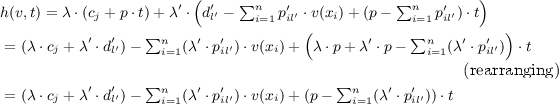
  $$\begin{aligned} h(v,t) = {\left\{ \begin{array}{ll} c_j+p \cdot t &{} \text {if } (v,t)\in F_j \cap H \\ d_{l'}'- \sum \nolimits _{i=1}^n p_{il'}' \cdot v(x_i) + \left( p - \sum \nolimits _{i=1}^n p_{il'}' \right) \cdot t &{} \text {if } (v,t) \in G_{l'}' \cap H' \end{array}\right. } \end{aligned}$$

  where

  $$\begin{aligned} H =&\; \{(v,t) \in \zeta \times \mathbb {R}\;|\;c_j+p \cdot t \le d_{l'}'- \sum \nolimits _{i=1}^n p_{il'}' \cdot v(x_i) + \left( p - \sum \nolimits _{i=1}^n p_{il'}' \right) \cdot t \} \\ =&\; \{(v,t) \in \zeta \times \mathbb {R}\;|\; \sum \nolimits _{i=1}^n p_{il'}' \cdot (v(x_i)+t) \le d_{l'}' - c_j \} \qquad \qquad {\text {(rearranging)}} \\ =&\; \{(v,t) \in \zeta \times \mathbb {R}\;|\; \sum \nolimits _{i=1}^n p_{il'}' \cdot (v+t)(x_i) \le d_{l'}' - c_j \} \quad (\text {by definition of}\ v+t) \end{aligned}$$

  and similarly $H' = \{(v,t) \in \zeta \times \mathbb {R}\;|\;\sum \nolimits _{i=1}^n -p_{il'}' \cdot (v+t)(x_i) \le c_j - d_{l'}' \}$.

• If $(v,t) \in G_l \cap F_{j'}'$ for some l and $j'$, then

  $$\begin{aligned} h(v,t) = {\left\{ \begin{array}{ll} d_l- \sum \nolimits _{i=1}^n p_{il} \cdot v(x_i) + \left( p - \sum \nolimits _{i=1}^n p_{il} \right) \cdot t &{} \text {if } (v,t) \in G_l \cap H \\ c_{j'}+t &{} \text {if } (v,t)\in F_{j'}' \cap H' \end{array}\right. } \end{aligned}$$

  and by a similar reduction to the case above we have:

  $$\begin{aligned} H =&\; \{(v,t) \in \zeta \times \mathbb {R}\;|\; \sum \nolimits _{i=1}^n -p_{il} \cdot (v+t)(x_i) \le c_{j'} - d_{l} \} \\ H' =&\; \{(v,t) \in \zeta \times \mathbb {R}\;|\; \sum \nolimits _{i=1}^n p_{il} \cdot (v+t)(x_i) \le d_{l} - c_{j'} \}. \end{aligned}$$

• If $(v,t) \in G_l \cap G_{l'}'$ for some l and $l'$, then

  $$\begin{aligned} h(v,t) = {\left\{ \begin{array}{ll} d_l- \sum \nolimits _{i=1}^n p_{il} \cdot v(x_i) + \left( p - \sum \nolimits _{i=1}^n p_{il} \right) \cdot t &{} \text {if } (v,t) \in G_l \cap H \\ d_{l'}'- \sum \nolimits _{i=1}^n p_{il'}' \cdot v(x_i) + \left( p - \sum \nolimits _{i=1}^n p_{il'}' \right) \cdot t &{} \text {if } (v,t) \in G_{l'}' \cap H' \end{array}\right. } \end{aligned}$$

  where

  

  by definition of $v+t$ and similarly we have:

  $$\begin{aligned} H' = \{(v,t) \in \zeta \times \mathbb {R}\;|\;- \sum \nolimits _{i=1}^n (p_{il} - p_{il'}') \cdot (v+t)(x_i) \le d_{l}- d_{l'}' \}. \end{aligned}$$

Since in each case H and $H'$ are k-bipolyhedra, if follows from Definition 12 that the lemma holds.    $\square$

The final operations performed by $T^{\min }_{{\mathtt {G}}_{\min }}$ and $T^{\max }_{{\mathtt {G}}_{\max }}$ concern taking the infimum or supremum over t of a function of the form $v \mapsto p \cdot t+f(l,\zeta )(l,v+t)$. Hence, we now show that performing either of these operations on a rational (p, k)-nice function returns a rational k-simple function.

Lemma 5

For any zone $\zeta$, if $g : (\zeta \times \mathbb {R}) {\rightarrow } \mathbb {R}$ is rational (p, k)-nice, then the functions $f_1 : \zeta {\rightarrow } \mathbb {R}$ and $f_2 : \zeta {\rightarrow } \mathbb {R}$ where $f_1(v) = \inf _{t\in \mathbb {R}} g(v,t)$ and $f_2(v) = \sup _{t\in \mathbb {R}} g(v,t)$ for $v \in \zeta$ are rational k-simple.

Proof

We prove the case for $f_1$; the case for $f_2$ follows similarly (swapping $\varDelta ^-$ and $\varDelta ^+$). Consider any zone $\zeta$ and rational (p, k)-nice function $g : (\zeta \times \mathbb {R}) {\rightarrow } \mathbb {R}$. By Definition 12, for any $(v,t) \in \zeta \times \mathbb {R}$, we have:

$$\begin{aligned} g(v,t) = {\left\{ \begin{array}{ll} c_j+p \cdot t &{} \text {if } (v,t)\in F_j \\ d_l- \sum \nolimits _{i=1}^n p_{il} \cdot v(x_i) + \left( p - \sum \nolimits _{i=1}^n p_{il} \right) \cdot t &{} \text {if } (v,t) \in G_l \end{array}\right. } \end{aligned}$$

where $c_j, d_l, p_{il} \in \mathbb {Q}$ and

$$\begin{aligned} F_j = \{( v,t) \;|\;v \in C_j \wedge v+t\in C_j' \} \quad \text {and} \quad G_l = \{( v,t) \;|\;v \in D_l \wedge v+t\in D_l' \} \end{aligned}$$

for some k-polyhedra $C_j, C_j', D_l$ and $D_l'$ for all $1 \le i \le n, 1 \le j \le M$ and $1 \le l \le N$ for some $M,N \in \mathbb {N}$.

For any k-polyhedron C, let

Following the arguments of [4], it follows that the functions $\varDelta ^-(\cdot ,C) : \zeta {\rightarrow } \mathbb {R}$ and $\varDelta ^+(\cdot ,C) : \zeta {\rightarrow } \mathbb {R}$ are both k-simple over k-polyhedra. If $f_1(v)=\inf _{t\in \mathbb {R}} g(v,t)$, for any $v \in \zeta$ we have $f_1(v)$ equals:

$$\begin{aligned} {\left\{ \begin{array}{ll} c_j &{} \text {if } v \in C_j \cap C_j' \\ c_j + p \cdot \varDelta ^-(v,C_j') &{} \text {if } v \in C_j \setminus C_j' \\ d_l- \sum \nolimits _{i=1}^n p_{il} \cdot v(x_i) &{} \text {if } v\in D_l \cap D_l' \text { and } p - \sum \nolimits _{i=1}^n p_{il} \ge 0 \\ d_l- \sum \nolimits _{i=1}^n p_{il} \cdot v(x_i) + \left( p - \sum \nolimits _{i=1}^n p_{il} \right) \cdot \varDelta ^-(v,D_l') \!\! &{} \text {if } v \in D_l \setminus D_l' \text { and } p - \sum \nolimits _{i=1}^n p_{il} \ge 0 \\ d_l- \sum \nolimits _{i=1}^n p_{il} \cdot v(x_i) + \left( p - \sum \nolimits _{i=1}^n p_{il} \right) \cdot \varDelta ^+(v,D_l') \!\! &{} \text {if } v \in D_l \text { and } p - \sum \nolimits _{i=1}^n p_{il} < 0 \end{array}\right. } \end{aligned}$$

In all except the final two cases, since $\varDelta ^-(\cdot ,C) : \zeta {\rightarrow } \mathbb {R}$ is k-simple, it follows that $f_1$ is rational k-simple. Considering the penultimate case, by definition of k-simple functions we have the following two cases to consider.

• if $\varDelta ^-(v,D_l')=d_l'$ for some $d_l' \in \mathbb {Q}_{+}$, then for any $v \in D_l \setminus D_l'$:

  $$\begin{aligned} f_1(v) =&\; d_l- \sum \nolimits _{i=1}^n p_{il} \cdot v(x_i) + \left( p - \sum \nolimits _{i=1}^n p_{il} \right) \cdot \varDelta ^-(v,D_l') \\ =&\; \big (d_l+ \left( p - \sum \nolimits _{i=1}^n p_{il} \right) \cdot d_l' \Big ) - \sum \nolimits _{i=1}^n p_{il} \cdot v(x_i) \,\,\qquad \qquad \text {(rearranging)} \end{aligned}$$

  which is rational k-simple, since g is rational (p, k)-nice.

• if $\varDelta ^-(v,D_l')= d_l' - v(x_{i_l'})$ for some $d_l' \in \mathbb {Q}_{+}$ and $1 \le i_l' \le n$, then for any $v \in D_l \setminus D_l'$:

  $$\begin{aligned} f_1(v) =&\; d_l- \sum \nolimits _{i=1}^n p_{il} \cdot v(x_i) + \left( p - \sum \nolimits _{i=1}^n p_{il} \right) \cdot \varDelta ^-(v,D_l') \\ =&\; d_l- \sum \nolimits _{i=1}^n p_{il} \cdot v(x_i) + \left( p - \sum \nolimits _{i=1}^n p_{il} \right) \cdot (d_l' - v(x_{i_l'})) \quad \text {(rearranging)} \\ =&\; \Big (d_l+ \left( p - \sum \nolimits _{i=1}^n p_{il} \right) \cdot d_l' \Big ) - \sum \nolimits _{i=1}^n p_{il}' \cdot v(x_i) \end{aligned}$$

  where $p_{il}' = p_{il} + (p - \sum \nolimits _{i=1}^n p_{il})$ if $i=i_l'$ and $p_{il}'=p_{il}$ otherwise.

The final case follows similarly to the penultimate using the fact $\varDelta ^+(v,D_l')$ is a k-simple function. Therefore, we can conclude that $f_1$ is rational k-simple as required.    $\square$

In the related proof of [25] we see that, for minimum expected time computation, it is always optimal to let as little time pass as possible in the current polyhedron and, for maximum expected time computation, it is always optimal to let as much time pass as possible. However, for prices, we see that this is not always the case, e.g., $\varDelta ^+(v,C)$ is used in the computation of minimum expected prices. This is due to the fact that price rates in locations reached at a later stage can be higher, and in such cases it can be optimal to let time pass now and accumulate a lower price, as opposed to waiting and accumulating a higher price later.

We now combine the above results and show that rational k-simple functions are a suitable representation for value functions when computing optimal expected time using value iteration and either $T^{\min }_{{\mathtt {G}}_{\min }}$ or $T^{\max }_{{\mathtt {G}}_{\max }}$.

Proposition 2

For $\mathrm {opt}\in \{ \min , \max \}$, if $f : {\mathtt {Z}}_{\mathrm {opt}} {\rightarrow } (S_{\mathrm {opt}} {\rightarrow } \mathbb {R})$ is a rational k-simple function, then $T^{\mathrm {opt}}_{{\mathtt {G}}_{\mathrm {opt}}}(f)$ is rational k-simple.

Proof

We only the consider when $\mathrm {opt}=\min$, the case when $\mathrm {opt}=\max$ follows similarly. Consider any rational k-simple function, ${\mathtt {z}}=(l,\zeta ) \in {\mathtt {Z}}_{\min }$ and $E \in {\mathtt {E}}({\mathtt {z}})$. For any $v \in \mathbb {R}^\mathcal {X}$ and $t \in \mathbb {R}$ and letting $r = \mathsf {price}_{L}(l)$ and $p' = \mathsf {price}_{ Act }(l,a)$:

$$\begin{aligned}&p \cdot t + p' + \sum \nolimits _{({\mathtt {z}},a,(R,l'),{\mathtt {z}}_{(R,l')}) \in E} \mathsf {prob}(l,a)(R,l') \cdot f({\mathtt {z}}_{(R,l')})(l',(v+t)[R]) \nonumber \\&\quad = p \cdot t + p' + \sum \nolimits _{({\mathtt {z}},a,(R,l'),{\mathtt {z}}_{(R,l')}) \in E} \mathsf {prob}(l,a)(R,l') \cdot f[R]({\mathtt {z}}_{(R,l')})(l',v+t) \nonumber \\&\qquad \qquad \qquad \qquad \qquad \qquad \qquad \qquad \qquad \text {(by Definition 11)} \nonumber \\&\quad = \sum \nolimits _{({\mathtt {z}},a,(R,l'),{\mathtt {z}}_{(R,l')}) \in E} \mathsf {prob}(l,a)(R,l') \cdot \left( p \cdot t + p' + f[R]({\mathtt {z}}_{(R,l')})(l',v+t) \right) \end{aligned}$$

(rearranging)

since $\mathsf {prob}(l,a)$ is a distribution. By construction, f is rational k-simple, and hence for any $({\mathtt {z}},a,(R,l'),{\mathtt {z}}_{(R,l')}) \in E$ using Lemmas 1 and 2 we have that $p' +f[R]$ is also rational k-simple. Using Definition 12 it follows that:

$$\begin{aligned} (v,t) \mapsto p \cdot t + p' + f[R]({\mathtt {z}}_{(R,l')})(l',v+t) \end{aligned}$$

is rational (p, k)-nice. Thus, since $({\mathtt {z}},a,(R,l'),{\mathtt {z}}_{(R,l')}) \in E$ was arbitrary, using Lemma 3 and (2) we have that:

$$\begin{aligned} (v,t) \mapsto p \cdot t + p' + \sum \nolimits _{({\mathtt {z}},a,(R,l'),{\mathtt {z}}_{(R,l')}) \in E} \mathsf {prob}(l,a)(R,l') \cdot f({\mathtt {z}}_{(R,l')})(l',(v+t)[R]) \end{aligned}$$

is also rational (p, k)-nice. Since $E \in {\mathtt {E}}({\mathtt {z}})$ was arbitrary and ${\mathtt {E}}({\mathtt {z}})$ is finite, Lemma 4 tells us:

$$\begin{aligned} (v,t) \mapsto \min _{E \in {\mathtt {E}}({\mathtt {z}})} \left\{ p \cdot t + p' + \sum \limits _{({\mathtt {z}},a,(R,l'),{\mathtt {z}}_{(R,l')}) \in E} \mathsf {prob}(l,a)(R,l') \cdot f({\mathtt {z}}_{(R,l')})(l',(v+t)[R]) \right\} \end{aligned}$$

is again rational (p, k)-nice. Finally, using Definition 6 and Lemma 5, it follows that $T_{{\mathtt {G}}}(f)({\mathtt {z}})$ is rational k-simple as required.    $\square$

Proposition 2 tells us that value iteration over a zone graph to compute expected prices, as specified in Definition 6, can be performed using rational k-simple functions (and rational (p, k)-nice functions).

4.3 Example

Figure 2 shows an example of a linearly-priced PTA. Location prices are indicated next to each location; all action prices are zero so they are omitted from the figure. For this example, we consider the target set $F=\{ l_2\}$ and compute both the minimum and maximum expected price of reaching F. For this PTA, all states reach the target with minimum (and maximum) probability 1, and therefore the zone graphs used for minimum and maximum expected price computation are the same and equal that constructed using the algorithm presented in Fig. 1. This zone graph is shown in Fig. 3.

Fig. 2.

Example PTA $\mathsf {P}$

Fig. 3.

Backwards zone graph ${\mathtt {G}}$ for PTA of Fig. 2 and target set $\{l_3\}$

In the case of the minimum expected price, performing value iteration over the zone graph ${\mathtt {G}}$ of Fig. 3 gives, for $n{\ge 3}$:

$$\begin{aligned} (T_{{\mathtt {G}}}^{\min })^n(f_0)({\mathtt {z}}_0)(l_0,v) =&\; \left( 2 + 0.5 \cdot \left( 3 + \sum \nolimits _{i=0}^{n-3} 0.25^i \right) \right) -v(x) \\ (T_{{\mathtt {G}}}^{\min })^n(f_0)({\mathtt {z}}_1)(l_1,v) =&\; {\left\{ \begin{array}{ll} 9-3 \cdot v(x) &{}\;\; {if }\,\, v(x) \le 3 \\ 0 &{}\;\; {if }\,\, 3 \le v(x) \le 4 \end{array}\right. } \\ (T_{{\mathtt {G}}}^{\min })^n(f_0)({\mathtt {z}}_2)(l_2,v) =&\; \sum \nolimits _{i=0}^{n-2} 0.25^i - v(x) \\ (T_{{\mathtt {G}}}^{\min })^n(f_0)({\mathtt {z}}_3)(l_3,v) =&\; 0 \end{aligned}$$

It then follows that the minimum expected price to reach the target from the initial state equals 4.166667. On the other hand, for the maximum expected price, performing value iteration yields for $n\ge 3$:

$$\begin{aligned} (T_{{\mathtt {G}}}^{\max })^n(f_0)({\mathtt {z}}_0)(l_0,v) =&\; {\left\{ \begin{array}{ll} \left( 1 + 0.5 \cdot \left( 9 + \sum \nolimits _{i=0}^{n-3} 0.25^i \right) \right) - v(x) &{} {if}\,\, x \le 1 \\ 0.5 \cdot \left( 12 + \sum \nolimits _{i=0}^{n-3} 0.25^i \right) - 3 \cdot v(x) &{} {if}\,\, 1 \le x \le 2 \\ \end{array}\right. }\\ (T_{{\mathtt {G}}}^{\max })^n(f_0)({\mathtt {z}}_1)(l_1,v) =&\; 12-3 \cdot v(x) \\ (T_{{\mathtt {G}}}^{\max })^n(f_0)({\mathtt {z}}_2)(l_2,v) =&\; \sum \nolimits _{i=0}^{n-2} 0.25^i - v(x) \\ (T_{{\mathtt {G}}}^{\max })^n(f_0)({\mathtt {z}}_3)(l_3,v) =&\; 0 \end{aligned}$$

and hence the maximum expected price for the initial state is 6.166667.

The optimal strategy for the minimum expected price is to always perform an action as soon as it is enabled. The choices of the optimal strategy for the maximum expected price are to leave $l_0$ as soon as the action a is enabled, as this allows it to remain longer in $l_1$, yielding a higher overall expected price.

5 Conclusions

We have extended the techniques of [25] for the symbolic computation of optimal expected time and strategy synthesis to expected prices for linearly-priced probabilistic timed automata. The approach involves building the backwards zone graph of the PTA under study and then performing value iteration over this graph. We have demonstrated that an extension of simple and nice functions over rational valued polyhedra provide an effective representation of the value functions required for this computation. One restriction that we impose on the linearly-priced PTAs we consider is that all location prices are positive. We note that it should be possible to remove this restriction by extending the algorithms of [17] for removing zero-priced end components for finite state MDPs to linearly-priced PTAs.

As already mentioned in [25], an important next step is to perform a rigorous investigation into the advantages and disadvantages of our approach in comparison with the digital clocks method [28]. This will require implementing the algorithms introduced here, for example using the Parma Polyhedra Library [5], which includes efficient ways of manipulating convex polyhedra and has already been used effectively to implement a number of real-time verification algorithms. Finally, we also plan to investigate policy iteration since it converges to optimal expected prices (see Theorem 1 and Corollary 1).

References

Alur, R., Courcoubetis, C., Dill, D.: Model checking in dense real time. Inf. Comput. 104(1), 2–34 (1993)
Alur, R., Dill, D.: A theory of timed automata. Theor. Comput. Sci. 126, 183–235 (1994)
Alur, R., Torre, S., Pappas, G.J.: Optimal paths in weighted timed automata. In: Di Benedetto, M.D., Sangiovanni-Vincentelli, A. (eds.) HSCC 2001. LNCS, vol. 2034, pp. 49–62. Springer, Heidelberg (2001). doi:10.1007/3-540-45351-2_8
Asarin, E., Maler, O.: As soon as possible: time optimal control for timed automata. In: Vaandrager, F.W., van Schuppen, J.H. (eds.) HSCC 1999. LNCS, vol. 1569, pp. 19–30. Springer, Heidelberg (1999). doi:10.1007/3-540-48983-5_6
Bagnara, R., Hill, P., Zaffanella, E.: The Parma Polyhedra Library: toward a complete set of numerical abstractions for the analysis and verification of hardware and software systems. Sci. Comput. Program. 72(1–2), 3–21 (2008)
Beauquier, D.: On probabilistic timed automata. Theor. Comput. Sci. 292(1), 65–84 (2003)
Behrmann, G., Fehnker, A., Hune, T., Larsen, K., Pettersson, P., Romijn, J., Vaandrager, F.: Minimum-cost reachability for priced time automata. In: Di Benedetto, M.D., Sangiovanni-Vincentelli, A. (eds.) HSCC 2001. LNCS, vol. 2034, pp. 147–161. Springer, Heidelberg (2001). doi:10.1007/3-540-45351-2_15
Bellman, R.: Dynamic Programming. Princeton University Press, Princeton (1957)
Berendsen, J., Chen, T., Jansen, D.N.: Undecidability of cost-bounded reachability in priced probabilistic timed automata. In: Chen, J., Cooper, S.B. (eds.) TAMC 2009. LNCS, vol. 5532, pp. 128–137. Springer, Heidelberg (2009). doi:10.1007/978-3-642-02017-9_16
Berendsen, J., Jansen, D., Katoen, J.-P.: Probably on time and within budget - on reachability in priced probabilistic timed automata. In: Proceedings of the 3rd International Conference Quantitative Evaluation of Systems (QEST 2006), pp. 311–322. IEEE Press (2006)
Berendsen, J., Jansen, D., Vaandrager, F.: Fortuna: model checking priced probabilistic timed automata. In: Proceedings of the 7th International Conference Quantitative Evaluation of Systems (QEST 2010), pp. 273–281. IEEE Press (2010)
Bertsekas, D.: Dynamic Programming and Optimal Control, vol. 1 and 2. Athena Scientific, Belmont (1995)
Bertsekas, D., Tsitsiklis, J.: An analysis of stochastic shortest path problems. Math. Oper. Res. 16(3), 580–595 (1991)
Bianco, A., de Alfaro, L.: Model checking of probabilistic and nondeterministic systems. In: Thiagarajan, P.S. (ed.) FSTTCS 1995. LNCS, vol. 1026, pp. 499–513. Springer, Heidelberg (1995). doi:10.1007/3-540-60692-0_70
Bohnenkamp, H., D’Argenio, P., Hermanns, H., Katoen, J.-P.: Modest: a compositional modeling formalism for hard and softly timed systems. IEEE Trans. Softw. Eng. 32(10), 812–830 (2006)
David, A., Jensen, P.G., Larsen, K.G., Legay, A., Lime, D., Sørensen, M.G., Taankvist, J.H.: On time with minimal expected cost!. In: Cassez, F., Raskin, J.-F. (eds.) ATVA 2014. LNCS, vol. 8837, pp. 129–145. Springer, Cham (2014). doi:10.1007/978-3-319-11936-6_10
de Alfaro, L.: Computing minimum and maximum reachability times in probabilistic systems. In: Baeten, J.C.M., Mauw, S. (eds.) CONCUR 1999. LNCS, vol. 1664, pp. 66–81. Springer, Heidelberg (1999). doi:10.1007/3-540-48320-9_7
Duflot, M., Kwiatkowska, M., Norman, G., Parker, D.: A formal analysis of Bluetooth device discovery. Int. J. Softw. Tools Technol. Transf. 8(6), 621–632 (2006)
Gregersen, H., Jensen, H.: Formal design of reliable real time systems. Master’s thesis, Department of Mathematics and Computer Science, Aalborg University (1995)
Hartmanns, A., Hermanns, H.: A modest approach to checking probabilistic timed automata. In: Proceedings of the 6th International Conference on Quantitative Evaluation of Systems (QEST 2009), pp. 187–196. IEEE Press (2009)
Henzinger, T.A., Manna, Z., Pnueli, A.: What good are digital clocks? In: Kuich, W. (ed.) ICALP 1992. LNCS, vol. 623, pp. 545–558. Springer, Heidelberg (1992). doi:10.1007/3-540-55719-9_103
Henzinger, T., Nicollin, X., Sifakis, J., Yovine, S.: Symbolic model checking for real-time systems. Inf. Comput. 111(2), 193–244 (1994)
James, H., Collins, E.: An analysis of transient Markov decision processes. J. Appl. Probab. 43(3), 603–621 (2006)
Jovanović, A., Kwiatkowska, M., Norman, G.: Symbolic minimum expected time controller synthesis for probabilistic timed automata. In: Sankaranarayanan, S., Vicario, E. (eds.) FORMATS 2015. LNCS, vol. 9268, pp. 140–155. Springer, Cham (2015). doi:10.1007/978-3-319-22975-1_10
Jovanovic, A., Kwiatkowska, M., Norman, G., Peyras, Q.: Symbolic optimal expected time reachability computation and controller synthesis for probabilistic timed automata. Theoret. Comput. Sci. 669, 1–21 (2017)
Kemeny, J., Snell, J., Knapp, A.: Denumerable Markov Chains. Springer, New York (1976)
Kwiatkowska, M., Norman, G., Parker, D.: PRISM 4.0: verification of probabilistic real-time systems. In: Gopalakrishnan, G., Qadeer, S. (eds.) CAV 2011. LNCS, vol. 6806, pp. 585–591. Springer, Heidelberg (2011). doi:10.1007/978-3-642-22110-1_47
Kwiatkowska, M., Norman, G., Parker, D., Sproston, J.: Performance analysis of probabilistic timed automata using digital clocks. Formal Methods Syst. Des. 29, 33–78 (2006)
Kwiatkowska, M., Norman, G., Segala, R., Sproston, J.: Automatic verification of real-time systems with discrete probability distributions. Theoret. Comput. Sci. 282, 101–150 (2002)
Kwiatkowska, M., Norman, G., Sproston, J., Wang, F.: Symbolic model checking for probabilistic timed automata. Inf. Comput. 205(7), 1027–1077 (2007)
Larsen, K., Pettersson, P., Yi, W.: Uppaal in a nutshell. Int. J. Softw. Tools Technol. Transf. 1, 134–152 (1997)
Larsen, K.G., Pettersson, P., Yi, W.: Model-checking for real-time systems. In: Reichel, H. (ed.) FCT 1995. LNCS, vol. 965, pp. 62–88. Springer, Heidelberg (1995). doi:10.1007/3-540-60249-6_41
Tripakis, S.: The analysis of timed systems in practice. Ph.D. thesis, Université Joseph Fourier, Grenoble (1998)
Tripakis, S.: Verifying progress in timed systems. In: Katoen, J.-P. (ed.) ARTS 1999. LNCS, vol. 1601, pp. 299–314. Springer, Heidelberg (1999). doi:10.1007/3-540-48778-6_18
Tripakis, S., Yovine, S., Bouajjani, A.: Checking timed Büchi automata emptiness efficiently. Formal Methods Syst. Des. 26(3), 267–292 (2005)
Acknowledgments
This work was partly supported by the EPSRC Mobile Autonomy Programme Grant EP/M019918/1 and the PRINCESS project, funded by the DARPA BRASS programme.
Author information
Authors and Affiliations
Corresponding author
Editor information
Editors and Affiliations
Rights and permissions
Copyright information
© 2017 Springer International Publishing AG
About this chapter
Cite this chapter
Kwiatkowska, M., Norman, G., Parker, D. (2017). Symbolic Verification and Strategy Synthesis for Linearly-Priced Probabilistic Timed Automata. In: Aceto, L., Bacci, G., Bacci, G., Ingólfsdóttir, A., Legay, A., Mardare, R. (eds) Models, Algorithms, Logics and Tools. Lecture Notes in Computer Science(), vol 10460. Springer, Cham. https://doi.org/10.1007/978-3-319-63121-9_15
Download citation
DOI: https://doi.org/10.1007/978-3-319-63121-9_15
Published:
Publisher Name: Springer, Cham
Print ISBN: 978-3-319-63120-2
Online ISBN: 978-3-319-63121-9
eBook Packages: Computer ScienceComputer Science (R0)