CBCT Use in Daily Practice

Scarfe, William C.; Angelopoulos, Christos

doi:10.1007/978-3-319-62061-9_5

William C. Scarfe B.D.S., F.R.A.C.D.S., M.S.³ &
Christos Angelopoulos D.D.S., M.S.^4,5

3980 Accesses
2 Citations

Abstract

Whilethere are some operational similarities between dental panoramic radiography and maxillofacial cone beam computed tomography (CBCT), the use of CBCT in daily practice necessitates that the clinician develop a higher level of technical competency in a variety of skill sets and radiologic interpretive expertise. The purpose of this Chapter is to underline the technical parameters by which practitioners can provide diagnostically acceptable images at the lowest reasonable dose by developing equipment specific exposure and acquisition protocols. To extract the most information from the CBCT scan, a generic algorithm is provided to optimize volumetric display. Specific image analysis functions and their appropriate applications as well as the prerequisites for radiologic reports are also presented. Finally, a comprehensive practical strategy for ensuring information optimized, minimal dose CBCT imaging is outlined.

Access provided by CONRICYT-eBooks. Download chapter PDF

Current Applications

History, Technique, and Safety

Clinical guidelines for dental cone-beam computed tomography

Article 11 January 2018

1 CBCT Operation

The operation and ease of use of maxillofacial CBCT equipment is technically simple and similar, in many respects, to dental panoramic radiography (DPR). In fact, since 2007, many DPR platforms are configured to provide additional CBCT functionality, sharing the same mechanical assembly and X-ray generator. This has led to some regulatory ambiguities regarding the categorization of dental and maxillofacial CBCT units as either dental or medical devices, and credentialing issues for facilities and personnel who operate this equipment. Operator requirements differ markedly between countries. For example, in many jurisdictions in the United States, maxillofacial CBCT devices are operated by dental auxiliaries with nominal radiographic qualifications, whereas in some European countries they can only be operated by dentists with special training.

While there are similarities between DPR and CBCT, a number of differences in acquisition and technique exist which distinguish the latter as a maxillofacial imaging modality that demands a higher level of technical competency and expertise. The operation of CBCT devices should be considered in two sequential and distinct phases (Fig. 5.1):

Scanning Protocol. The choice of specific technical parameters to optimize image quality and minimize exposure for a specific imaging task is called the imaging acquisition or scan protocol. Perhaps the greatest distinction between DPR and CBCT imaging lies in the fact that CBCT provides the operator with the choice of many more technique variables (Table 5.1). Practitioners and operators using CBCT must have a thorough understanding of the available operational exposure and acquisition parameters and the effects of these parameters on image quality and radiation safety (Carter et al. 2008).
Table 5.1 Comparison of the similarities and differences between the operation and techniques of DPR and maxillofacial CBCT devices
Full size table

Image Protocol. Once acquired, it is necessary to interact with volumetric CBCT data to optimize image display on the monitor. The principle components of this are to reorient the data, enhance the data, and then to reformat the data so that the clinician can explore, analyze, and interpret the volume (See Sect. 5.2).

1.1 Scan Protocol

1.1.1 Exposure Factors

Four exposure parameters determine the quality and quantity of the X-ray beam. Two of the factors, focal spot size and beam frequency, are equipment dependent and fixed whereas the other two, milliamperes (mA) and kilovoltage (kV), may be variable and are operator controlled.

1.1.1.1 Equipment Dependent

The following factors should be considered when purchasing a CBCT unit and while are not specifically adjusted clinically, do introduce potential limitations on image quality and patient radiation dose optimization:

Focal spot size. Focal spot size is one parameter that determines the penumbra or geometric unsharpness of CBCT image formation. CBCT units with smaller focal spot sizes theoretically produce less penumbra and consequently sharper images. Most CBCT units have a nominal focal spot of 0.5 mm; however, some are lower at 0.3 mm with the lowest at 0.15 mm. Lower focal spot size has two disadvantages.
- The maximum field of view (FOV) of the CBCT unit may be limited because of increased projection divergence at the peripheral of the X-ray beam.
- Low mAs must be used or otherwise a longer duty cycle is necessary, especially with greater numbers of basis images, so as to not overheat the generator.
X-ray Generator Frequency. In most CBCT units, X-ray generation is pulsed to coincide with the detector activation. Pulsed X-ray beam generation is preferable to continuous exposure as it markedly reduces total exposure scan time with less radiation dose to the patient. In addition, there is diminished heat production at the anode and reduces the impact of detector afterglow. However, the relatively low power used in this type of X-ray generator provides some limitations in image quality. Continuous exposure units produce X-ray spectra with a higher peak kV and capable of faster acquisition of a greater number of basis frames with theoretically less image noise.

1.1.1.2 Operator Controlled

CBCT manufacturers approach setting exposure factors in one of three ways.

Fixed. Operators are offered a selection of predetermined or “fixed” exposure setting combinations (e.g., PreXion, PreXion Co., Ltd, Tokyo, Japan; GALILEOS, Sirona AG, Bensheim, Germany; Newtom5g/VGi, QR, Inc. (a Cefla Company), Milano, Italy).
Variable. Operators can manually adjust kV and/or mA settings. Operators who use CBCT units with operator adjustable exposure settings should be aware that these parameters affect both image quality (See Chap. 2) and have patient radiation dose consequences. Careful selection is required to fulfill the ALARA (As Low As Reasonably Achievable) principle. Manufactures may incorporate “preset” exposure settings for different sized individuals (Fig. 5.2) or specific imaging scan protocols (Fig. 5.3).
Fig. 5.2
Screen shot of exposure panel for a CBCT device (RayScan Alpha, LED Medical Diagnostics Inc., Vancouver, British Columbia, Canada) that adjusts exposure settings for different sized individuals. Exposure settings for a high definition scan (HD) of the dentition, (highlighted occluding teeth icon) for an “average” sized individual (a) (90 kVp and 11 mA) is higher than that for a child (b) (85 kVp and 10 mA)
Full size image

Fig. 5.3
Screen shot of exposure panel for a CBCT device (Accuitomo 170, J. Morita, Kyoto, Japan) that has default exposure settings based on number of basis projection images. Manufacturer default exposure settings for a 360° standard (Std), 80 mm × 80 mm scan (HD) (a) (90 kVp and 5 mA), is identical to that of a 360° standard (Std) with a smaller FOV (40 mm × 80 mm) (b). Exposure settings for a 360° 80 mm × 80 mm scan with a greater number of basis projection images (HiFi) (c) requires an increased mA setting (7 mA)
Full size image
Automatic Exposure Control. Automatic exposure control (AEC) is a dose reduction strategy used in most MDCT devices to optimize patient doses. AEC attempts to adjust and customize (i.e., modulate) tube current (mA) specifically for each patient according to the radiation intensity detected by using a short pre-examination (scout) exposure (NewTom-FP; Quantitative Radiology s.r.l., Cefla Group, Verona, Italy) or using a exposure modulation during the rotation (SafeBeam™ technology, NewTom VGI evo/NewTom GiANO, Quantitative Radiology s.r.l., Cefla Group, Verona, Italy) (Pauwels et al. 2014a, b; Pauwels et al. 2015a, b, c). It is expected that widespread implementation of AEC in CBCT will avoid the need for manual adaptation of exposure parameters based on patient size (Pauwels et al. 2012).

1.1.1.2.1 Effects of Exposure Setting Adjustments

Manufacturer recommended default exposure settings should be adjusted with caution as each parameter has effects on the image quality and patient radiation exposure (Goulston et al. 2016). Any exposure setting adjustment should be directed towards reducing exposures to levels as low as diagnostically acceptable (ALADA principle), particularly for children (White et al. 2014).

mA. The range of mA settings in available CBCT devices is extensive with most operating at less than 12 mA while some operate as high as 20 mA. mA may be adjustable on some units with higher levels producing darker images with less noisy image. However, patient effective dose increases proportionately, almost in a 1:1 ratio.
kV. Most CBCT units operate in the range less than 90 kV, whereas a few can operate at higher kV, up to 120 kV. The effect of kVp on dose and image quality is more intricate owing to a combination of several energy-dependent X-ray interactions (See Chap. 2). Higher kV units theoretically produce images with a higher contrast-to-noise ratio, particularly at lower exposures because of increased photon count and a decreased absorption ratio (Pauwels et al. 2014a, b). Adjustment of kV has an even greater effect on dose than does mA, with each decrease in 10 kV approximately halving dose if all other parameters remain the same (Pauwels et al. 2014a, b). In general, low kV units operate at higher mA.

The effect of changing one or both exposure factors on image quality and dose is not straightforward and should be balanced, ensuring that an adequate image quality is achieved at the lowest possible dose level. Currently (2017) there is still a low level of evidence on the effect of adjusting exposure settings (Goulston et al. 2016). Exposure setting adjustments may be considered in the following situations:

Patient size. In clinical practice, mA changes are preferable to kVp changes to compensate for differences in patient size as the increase in noise for a given dose reduction is smaller formA adjustments. Smaller patients (e.g., children) can be exposed using a lower (20–30% less) mA and produce images of acceptable diagnostic quality as for larger patients (Pauwels et al. 2015c, 2017).
Diagnostic task. For specific diagnostic tasks requiring reduced image quality, mA can be reduced without reducing diagnostic efficacy (Pauwels et al. 2015c). Significant dose reductions can be achieved by reducing tube current by up to 50% without substantial loss of diagnostic quality for relatively low-resolution tasks such as assessment of the paranasal sinuses (Güldner et al. 2013), presurgical implant planning (Sur et al. 2010; Dawood et al. 2012; Panmekiate et al. 2012; Bohner et al. 2017), or orthodontic diagnosis (Kwong et al. 2008). However, for diagnostic tasks requiring images with optimal image quality, mA can be increased. For example, dental periapical diagnosis involving visualizing the periodontal ligament space and subtle changes in bone trabeculation may benefit from moderate increases in mA producing images with reduced noise.

Similarly, a higher kVp may be considered in patients with high-density objects, such as teeth with root canal fillings (Chindasombatjareon et al. 2011; Vasconcelos et al. 2015; Helvacioglu-Yigit et al. 2016) or dental implants (Panjnoush et al. 2016; Vasconcelos et al. 2017), as beam hardening artifacts from these materials may be reduced. Conversely, lower kVp settings may also be considered for low discriminating diagnostic tasks such as orthodontics (Kwong et al. 2008).

1.1.2 Acquisition Parameters

1.1.2.1 Scan Time

The number of images comprising the projection data throughout the scan is determined by the frame rate (number of images acquired per second), the completeness of the trajectory arc, and the speed of the rotation. CBCT units may be configured to have a fixed or variable number of projection basis images comprising a single scan. This is usually referred to as scan time. Within the cost limitations of solid-state detectors used in CBCT construction and the need for short scanning time in a clinical setting, the number of images available for construction ranges from 150 to over 1000.

Increasing scan time provides more information to reconstruct the image and has multiple beneficial effects on the image including greater contrast resolution, improved signal-to-noise ratio producing “smoother” images, and reduces metallic artifacts (Fig. 5.4). This is usually associated with a longer duty cycle between patients to allow for cooling of the generator tube and a longer primary reconstruction time. For a given CBCT unit, a greater number of projections increases the amount of radiation a patient receives linearly—a scan comprising 1000 basis images delivers 2× the radiation dose to the patient than a scan reconstructed from 500 basis images. In accordance with the ALARA principle, the number of basis images should be optimized to produce an image of diagnostic quality considering the diagnostic task. Increasing scan time may be considered for patients with high-density objects within the FOV, such as dental implants (Nardi et al. 2015), as artifacts from these materials may be reduced. However, this improvement in image quality may be negated by the possibility of motion artifacts (Nardi et al. 2015) and the introduction of inconsistencies in gray density measurements (Parsa et al. 2013).

1.1.2.2 Relationship Between Scan, Exposure, and Reconstruction Time

Most CBCT units acquire all projection images in a single rotation. The actual period in which the gantry revolves around the patient’s head, or scan time, ranges from ~5 s to, at most, 40 s (Nemtoi et al. 2013). The total time that the X-ray generator is producing x-radiation for pulsed CBCT units, exposure time, is less than the actual scan time. This ranges from 2 s to approximately 12 s, with a maximum of up to 34 s.

Ideally, scan time should be comparable to panoramic radiography so that artifacts associated with subject movement are minimized. However, motion artifacts are common, reportedly ranging from 21 to 42% of CBCT examinations (Spin-Neto et al. 2015; Nardi et al. 2015). Correction algorithms to adjust for small patient movements and reduce the effects of motion artifacts have been proposed (Schulze et al. 2015) and advertised (Planmeca CALM™; Planmeca OY, Helsinki Finland) but as of 2017, not yet implemented. Different types of movements induce different artifacts, in different parts of the anatomy (Nardi et al. 2016). Artifacts can be described as smearing, double contour (Fig. 5.5), cancellous bone fading resulting from loss of trabeculae visibility and general unsharpness (Fig. 5.6). In general, movement of short duration may lead to double contours (bilateral or monolateral depending upon the angle of the scan at which they occur), whereas gradual movements result in blurring. The plane in which the artifact is most pronounced corresponds with the direction in which the movement occurs.

Reconstruction time is the time taken by the workstation computer for dataset reconstruction and varies depending on FOV, the number of basis images acquired, resolution and reconstruction algorithm and ranges from less than 30 s to over 5 min. The application of secondary reconstruction methods, such as iterative reconstruction for streak artifact reduction, can run considerably more than 5 min (Dong et al. 2013).

1.1.2.3 Rotation Angle

Most reconstruction algorithms (e.g., FDK algorithm) require that projection data is acquired from a complete circular trajectory of 360°. This rotational angle is also called the scan arc or orbital angle. However, it is possible to reduce the rotation angle of the CBCT gantry and still reconstruct a volumetric dataset. This approach potentially reduces the scan time and allows the robotic arm of a panoramic platform to provide the gantry motion for CBCT imaging. Images produced by this method may have greater noise and suffer from reconstruction interpolation artifacts (Fig. 5.7). CBCT systems may therefore have three rotational angle configurations: (1) Fixed full (360°) trajectory, (2) Full but variable, usually with two trajectory settings, or (3) Fixed partial (Table 5.2).

Table 5.2 Rotational arcs of various CBCT Units (Based on data from Nemtoi et al. (2013) and current manufacturer websites)

Full size table

For most diagnostic tasks, CBCT should be performed using the greatest scan arc available. In those units that provide reduction of rotation angle, degradation in image quality (Al-Okshi et al. 2017) may be offset by considerations of a proportionate reduction in patient radiation dose (Pauwels et al. 2014b). Reduction of trajectory arc is not recommended for the assessment of periodontal structures (Al-Okshi et al. 2017) and introduces inconsistency in grayscale density values (Parsa et al. 2013) however, may be considered for periapical diagnosis and implant planning (Lofthag-Hansen et al. 2011).

1.1.2.4 Field-of-View (FOV)

The volume of tissue of the patient’s head irradiated during exposure is referred to as the FOV or scan volume. The dimension of the FOV is primarily dependent on the detector size and shape, beam projection geometry, and beam collimation. The shape of the scan volume is determined by the sensor technology and acquisition method.

Spherical FOVs are characteristic of image intensifier detectors. Most flat panel detector (FPD) systems produce a cylindrical FOV with a height and circular diameter. A few devices limit the FOV to the jaw shape, restricting the region of interest (ROI) to the dental structures. The CS 9000 3D (Carestream, Atlanta, Georgia, USA) stitches three cylindrical FOVs from consecutive exposures in the horizontal axis enough to cover a single jaw. An alternate method to cover the shape of the jaws is provided by the Accuitomo R100 (J. Morita Corporation, Kyoto, Japan) (Fig. 5.8). This maxillofacial CBCT device is the only unit which produces a convex triangular shape from a complex motion of the gantry during exposure, referred to as 3D Reuleaux Full Arch (patent pending; J. Morita Corporation, Kyoto, Japan).

Collimation of the primary X-ray beam limits x-radiation exposure only to the region of interest (ROI). Effective dose ranges for field of views (FOVs) with height ≤ 5 cm between 9.7 and 197.0 μSv, for FOVs of heights 5.1–10.0 cm between 3.9 and 674.0 μSv, and for FOVs >10 cm between 8.8 and 1073.0 μSv (Al-Okshi et al. 2015). An optimal FOV should be selected for each patient based on diagnostic task and the region of interest (ROI).

Reduction in the FOV usually can be accomplished mechanically or, in some instances, electronically. Mechanical reduction in the dimensions of the X-ray beam can be achieved by either pre-irradiation (reducing primary radiation dimensions) or post-irradiation (reducing the dimensions of the transmitted radiation, before it is detected) collimation. Currently most CBCT units use adjustable metallic shields as primary collimation at the radiation source. Electronic collimation involves elimination of data recorded on the detector peripheral to the area of interest. In this case there is no physical reduction in irradiation of the ROI by physical means. Both techniques reduce the amount of data for computational purposes and reduce reconstruction time; however, only pre-irradiation physical collimation results in reduced patient radiation exposure.

Effects of FOV size on image quality can be seen in some circumstances (Fig. 5.4). Larger FOVs increase the amount of scatter per detector area, reducing image quality (Lofthag-Hansen et al. 2011). In addition, larger FOVs coincide with a higher beam divergence at the edge of the FOV, which results in image quality deterioration. On the other hand, a FOV with a larger diameter reduces the “local tomography” effect of tissue outside the FOV (which is only partially exposed) on gray value uniformity. While an FOV height of 4–6 cm may be adequate for a mandibular scan, an FOV height of 8 cm or even up to 10 cm may be advisable for the maxilla if sinus augmentation procedures are anticipated to adequately demonstrate the ostiomeatal complex.

1.1.2.5 Resolution

Contrast Resolution. The contrast resolution (ability to detect subtle differences in attenuation by differences in gray-level intensity) is device dependent and is influenced by several interacting acquisition variables (see Chap. 2). Maxillofacial CBCT images lack adequate grayscale sensitivity to discern subtle differences between soft tissues, such as between fluids and solid tumors, though are excellent for demonstrating air to soft tissue boundaries. Grayscale intensity values from CBCT images do not directly represent Hounsfield units (HU), the relative density of body tissues according to a calibrated gray-level scale, based on normalized-HU values for air (−1000 HU), water (0 HU), and dense bone (+1000 HU) (Bryant et al. 2008; Nackaerts et al. 2011; Molteni 2013). Several techniques and devices are currently being investigated to compensate for the deficiencies of CBCT acquisition such that derive gray density levels more accurately correlate with HU (Lagravere et al. 2006, 2008; Mah et al. 2010; Molteni 2013).
Spatial Resolution. The spatial resolution of maxillofacial CBCT systems is primarily a function of detector nominal pixel size and fill factor; however, many interrelated factors contribute to the final maximum achievable resolution (see Chap. 2). Most manufacturers provide options for varying resolution of CBCT data. However, the number of pixels within the area matrix of a sensor that capture x-rays is fixed. For a given projection geometry and FOV, the acquired dataset is always acquired at the highest, default resolution. In some CBCT units, resolution can be increased by altering projection geometry, reducing the object to focal spot distance. More often, electronic pixel binning is used to provide reconstructed images with voxel resolution less than that acquired. Pixel binning is the process of combining charge from adjacent electronic “wells” from the detector during readout. The two primary benefits of binning are improved contrast due to an improved signal-to-noise ratio and the ability to increase frame rate, albeit at the expense of reduced spatial resolution.

Higher resolution may be considered desirable for many tasks in dentistry demanding accuracy to the level of the detail of approximately the periodontal ligament space (i.e., approximately 0.2 mm or less) (Fig. 5.9). Images taken at high resolution often have reduced brightness and contrast, increased noise (when displayed in thin slice thickness), and require increased reconstruction time. While increased image resolution in some maxillofacial CBCT units does not affect changes in exposure parameters, some manufacturers incorporate reduced-dose exposure protocols for low-resolution settings.
Fig. 5.9
Default display of a dental imaging software (InVivo, Anatomage, San Jose, California USA) showing orthogonal projections and volumetric rendering of two CBCT examinations—one performed at 0.4 mm (a) and a second at 0.08 mm voxel resolution (b)—for an individual with bilateral impacted and unerupted maxillary canines. Orthogonal images at the higher resolution (b) more clearly show the periodontal ligament space and subtle root resorption associated with the adjacent lateral incisors
Full size image

As CBCT data is inherently volumetric, it is possible to resample the dataset to provide images with higher resolutions than originally reconstructed. This is known as reconstructed resolution. Previous iCAT models (Classic and Next-Generation (17/19), Imaging Sciences International, Hatfield, PA, USA) and the current 3D Accuitomo 170 (J. Morita Corp., Kyoto, Japan) allow for reconstructed resolution. The 3D Accuitomo 170 “zoom reconstruction” feature is unique in that for large FOV acquisitions, often displayed at low resolutions to reduce reconstruction time and file size, a small region of interest within the original scan can be identified and a small FOV with an 80 μm voxel resolution can be reconstructed from the original data (Fig. 5.10). As with other forms of digital radiography, acquired nominal resolution based on specified physical pixel or voxel values should be distinguished from the actual acquired resolution achieved due to the various constraints within the total imaging chain and reconstructed resolution.
Fig. 5.10
Cross-sectional, axial, and parasagittal maxillofacial CBCT orthogonal images (3D Accuitomo 170, J. Morita Corp., Kyoto, Japan) (a) of a mandibular left root canal filled second molar for a patient who presents with local pain and suspicion of a fractured tooth. A cropped, magnified sagittal image at the standard resolution (0.25 mm voxel size) (b) shows an apical hypodensity and associated furcation bone loss. Reconstructed resolution or “zoom reconstruction” was applied to a limited spherical region within the FOV of the original volumetric dataset (yellow circle—a). Comparable sagittal image of the reconstructed volume (c) at a higher 0.08 mm voxel resolution demonstrates a root fracture through the cervical portion of the mesial root extending into the furcation (arrows) accounting for the failure of the root canal treatment
Full size image

1.1.2.6 Calibration

Maxillofacial CBCT acquisition and image reconstruction result from a balance and coordination of an invariant and reproducible rotational geometric relationship between the X-ray generator and image sensor and the fidelity of the image sensor (Wischmann et al. 2002). Any disruption or disturbance in this geometric relationship, degradation of the image sensor, or variabilities in the preprocessing reconstruction algorithm will produce any number of scanner-related artifacts (See Chap. 2) (Schulze et al. 2011; Pauwels et al. 2015a).

Optimal image quality should incorporate a quality assurance (QA) plan including periodic calibration of both geometric and electronic components (see Chap. 7) (Vassileva and Stoyanov 2010; Health Protection Agency 2010). Tube- or detector-related geometric mismatch (Fig. 5.11) or preprocessing algorithmic incongruities (Fig. 5.12) may produce variations in signal intensities resulting in obvious or subtle disruptions in anatomic structures. Geometric artifacts are of particular importance in CBCT systems that use X-ray beam projection and sensor offset or data stitching techniques to increase the region of interest with a smaller sensor (See Chap. 2). Local artifacts in the digital sensor induce (usually circular) artifacts in the reconstructed slices (Fig. 5.13). The geometric accuracy of the CBCT unit should be regularly checked by use of a specific QA device. Calibration requires the absence of any object between the X-ray source and sensor, otherwise “ghost shadows” of the object will be present in subsequent images (Fig. 5.14).

2 Generic Steps to Optimize Volumetric Data Display

Most dental imaging software programs present CBCT data on the monitor with a default display. This is commonly as a series of three panes demonstrating secondary planar reconstructed images in one of each of three orthogonal planes (axial, sagittal, and coronal) at a defaulted thickness with a fourth pane demonstrating a volumetric image (Fig. 5.15). Each panel of the display software presents one of a series of contiguous images in that plane. Each image is interrelational such that the location of the image in the sequence within the volume can be identified in each of the other two planes.

CBCT data should be considered as a volume to be explored from which selective images are extracted. Consequently volumetric data is reformatted depending on the diagnostic task for which the acquisition was performed. As a rule of thumb for formatting, thin images provide structure detail whereas thick images provide structural relationships.

Technically four generic steps provide an efficient and consistent systematic and methodological approach to optimize CBCT image display prior to image interpretation. This approach is not equally applicable to all dental software, but serves as a guide to improve the visibility of anatomic structures.

2.1 Reorient the Data

The first step in optimizing display of the volumetric dataset is to ensure that the orthogonal projections provide an adequate representation of the imaged object. This requires that the orthogonal planes are perpendicular to the area of interest. This geometric transformation is important in various clinical scenarios including minimizing parallax error in the measurement of alveolar bone height (Fig. 5.16), detection of the inferior alveolar canal and its relationship to the roots of the third molar (Fig. 5.17), and assessment of craniofacial anomalies (Fig. 5.18).

Before proceeding in correcting, exploring, and reformatting volumetric data, it is important to apply a spatial geometric transformation to align the orthogonal planes to a standard orientation. As CBCT volumetric datasets are isotropic, dental imaging software may provide one of two methods to achieve this:

Reorient the volume. The entire volume can be reorientated such that the patient’s anatomic features are realigned to specific orthogonal reference planes (e.g., InVivo, Anatomage, San Jose, California USA; NNT 6.0, QR Verona, Verona, Italy and: Dolphin Imaging, Dolphin Imaging and Management Solutions, Chatsworth, California, USA) (Figs. 5.19 and 5.20).
Fig. 5.19
Example of default dental software display (InVivo, Anatomage, San Jose, California, USA) before (a) and after (b) adjustment of axial, sagittal, and coronal planes. In this software the orientation of the volume, as shown by the volumetric rendering (lower right) is reoriented using arrows (open red) associated with the respective panes to more accurately represent the entire maxillofacial region
Full size image

Fig. 5.20
Example of default dental software display (Galaxis, Dentsply Sirona Imaging, Bensheim, Germany) before (a) and after (b) adjustment of parasagittal (called tangential) and coronal (called cross-sectional) planes. In this software the orientation of the volume, as shown by the volumetric rendering (upper right), remains the same and the coronal (cross-sectional) and parasagittal (tangential) planes are adjusted using sliders to adjust the respective panes to more accurately represent the available edentulous area in the right mandibular molar region
Full size image
Reorient the orthogonal planes. Alternately, the volumetric dataset remains visually invariant and the orthogonal planes are adjusted (e.g., Galaxis/Sidexis 4, Dentsply Sirona Imaging, Bensheim, Germany; OnDemand3D, CyberMed, Seoul, Korea; NNT 6.0, QR Verona, Verona, Italy; and Kodak Dental Imaging Software 3D module [KDIS], Carestream, Atlanta, Georgia, USA) (Figs. 5.20, 5.21, 5.22 and 5.23).
Fig. 5.21
Example of default dental software display (OnDemand3D, CyberMed, Seoul, Korea) before (a) and after (b) adjustment of axial, sagittal, and coronal planes. In this software the orientation of the volume, as shown by the volumetric rendering (lower right), remains the same and the orthogonal planes are adjusted using the superimposed multipurpose cross-hairs (blue lines) associated with the respective panes to symmetrically reorient the planes to the entire maxillofacial region
Full size image

Fig. 5.22
Example of default software display (NNT 6.0, QR Verona, Verona, Italy) showing (a) the axis reorientation screen enabling the user to rotate the imaging volume with respect to the three orthogonal planes. An alternate screen (b) shows a different function of the NNT software that permits the reconstruction of multiple oblique non-orthogonal planes based on the diagnostic need. In this example, an oblique section of the maxillary right posterior region is identified by orienting the green line on the upper left pane and a parasagittal image reconstructed (lower right pane)
Full size image

Fig. 5.23
Example of default dental software display (KDIS 3D module, Carestream, Atlanta, Georgia, USA) before (a) and after (b) adjustment of axial (orange), sagittal (turquoise), and coronal (purple) planes. In this software the orientation of the volume, as shown by the volumetric rendering (upper right), remains the same visually and the orthogonal planes are adjusted using the superimposed cross-hairs (orange, purple, and green lines) associated with the respective orthogonal images to symmetrically reorient the planes to the entire maxillofacial region
Full size image

Many planes on interrelational orthogonal displays may be used for reference.

Sagittal Planes. The following planes can be used to adjust the vertical (y–z) axis:
- Inferior alveolar canal (IACP) plane. Parasagittal plane transecting the length of the IAC in the region of the mandibular third molar. Used in third molar assessments (Fig. 5.24)
  Fig. 5.24
  Example of default dental software display (KDIS 3D module, Carestream, Atlanta Georgia, USA) showing the adjustment of the sagittal, coronal, and axial planes relative to the inferior alveolar canal plane (IACP, orange) and resultant orthogonal images
  Full size image
- Midsagittal plane (MSP). Plane transecting the middle of the hard palate, anterior nasal spine, crista galli, and the middle of the occipital basilar bone. Used in orthodontic assessments (Fig. 5.25).
  Fig. 5.25
  Example of default dental software display (KDIS 3D module, Carestream, Atlanta Georgia, USA) showing the adjustment of the sagittal, coronal, and axial planes relative to the midsagittal plane (MSP, turquoise) and resultant orthogonal images
  Full size image
- Long axis of the tooth (LATs). Parasagittal plane transecting the long axis of the tooth (middle of the occlusal surface/incisal edge and apical terminus of the root of the tooth) (Fig. 5.26).
  Fig. 5.26
  Example of default dental software display (KDIS 3D module, Carestream, Atlanta Georgia, USA) showing the adjustment of the sagittal, coronal, and axial (orange) planes relative to the long axis of the tooth (LATs, turquoise; LATc, purple; LATa, orange) and resultant orthogonal images
  Full size image
Axial Planes. The following planes can be used to adjust the horizontal (x–z) axis:
- Frankfort Horizontal (FH). The imaginary plane transecting the most superior extent of the external auditory meatus and the most inferior portion of the orbital rim bilaterally. Used in orthodontic assessments (Fig. 5.27).
  Fig. 5.27
  Example of default dental software display (KDIS 3D module, Carestream, Atlanta Georgia, USA) showing the adjustment of the sagittal, coronal, and axial (orange) planes relative to Frankfort Horizontal (FH, orange) and resultant orthogonal images
  Full size image
- Intercondylar plane (ICPa). Imaginary axial plane transecting the medial or lateral poles of the mandibular condyles and parallel to FH. Used in TMJ assessment (Fig. 5.28).
  Fig. 5.28
  Example of default dental software display (KDIS 3D module, Carestream, Atlanta Georgia, USA) showing the adjustment of the sagittal, coronal, and axial (orange) planes relative to the axial and coronal intercondylar plane (ICPa, orange; ICPc, purple) and resultant orthogonal images
  Full size image
- Occlusal plane (OP). Imaginary plane transecting and parallel to the occlusal surfaces of the crowns of the teeth equally bilaterally (Fig. 5.29).
  Fig. 5.29
  Example of default dental software display (KDIS 3D module, Carestream, Atlanta Georgia, USA) showing the adjustment of the sagittal, coronal, and axial (orange) planes relative to the occlusal plane (OP, orange) and resultant orthogonal images
  Full size image
- Palatal plane (PP). Imaginary plane transecting and parallel to the hard palatal (Fig. 5.30).
  Fig. 5.30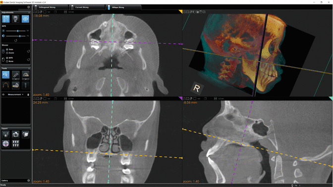
  Example of default dental software display (KDIS 3D module, Carestream, Atlanta Georgia, USA) showing the adjustment of the sagittal, coronal, and axial (orange) planes relative to the palatal plane (PP, orange) and resultant orthogonal images
  Full size image
- Long axis of the tooth (LATa). Axial plane transecting the long axis of the tooth (middle of the occlusal surface/incisal edge and apical terminus of the root of the tooth) (Fig. 5.25).
Coronal Planes. The following planes can be used to adjust the vertical (y–x) axis:
- Interorbital plane (IOP). An imaginary coronal plane transecting the most anterior-inferior portion of the orbital rim bilaterally and perpendicular to FH (Fig. 5.31).
  Fig. 5.31
  Example of default dental software display (KDIS 3D module, Carestream, Atlanta, Georgia, USA) showing the adjustment of the sagittal, coronal, and axial planes relative to the interorbital plane (IOP, purple) and resultant orthogonal images
  Full size image
- Infraorbital foraminae plane (IOFP). The imaginary plane transecting the infraorbital foramina bilaterally and perpendicular to FH (Fig. 5.32).
  Fig. 5.32
  Example of default dental software display (KDIS 3D module, Carestream, Atlanta, Georgia, USA) showing the adjustment of the sagittal, coronal, and axial planes relative to the infraorbital foraminae plane (IOFP, purple) and resultant orthogonal images
  Full size image
- Intercondylar plane (ICPc). Imaginary coronal plane transecting the medial or lateral poles of the mandibular condyles. Used in TMJ assessment (Fig. 5.28).
- Inter-porionic axis (IPAc). Imaginary coronal plane transecting the most superior aspect of the external auditory meati (EAM) bilaterally and perpendicular to FH (Fig. 5.33).
  Fig. 5.33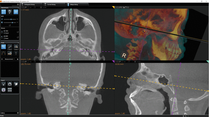
  Example of default dental software display (KDIS 3D module, Carestream, Atlanta, Georgia, USA) showing the adjustment of the sagittal, coronal, and axial (orange) planes relative to the Inter-porionic axis (IPA, purple) and resultant orthogonal images
  Full size image
- Long axis of the tooth (LATc). Paracoronal plane transecting the long axis of the tooth (middle of the occlusal surface/incisal edge and apical terminus of the root of the tooth) (Fig. 5.26).

For full volume scans, reorientation usually conforms to cephalometric reference planes (Table 5.3) (Figs. 5.34 and 5.35) whereas for limited volume scans and certain MPR reformations, the specific region of interest should be reoriented to regional reference planes (Tables 5.4, 5.5, 5.6, 5.7, 5.8 and 5.9) (Figs. 5.36, 5.37, 5.38, 5.39, 5.40, 5.41 and 5.42).

Table 5.3 Reference planes used to reorient full FOV CBCT volumetric datasets (craniofacial deformities, cephalometric analysis, and asymmetry) (Figs. 5.34 and 5.35)

Full size table

Table 5.4 Reference planes used to reorient limited FOV CBCT volumetric datasets of both the maxilla and mandible (Fig. 5.36)

Full size table

Table 5.5 Reference planes used to reorient limited FOV CBCT volumetric datasets of the TMJ (Fig. 5.37)

Full size table

Table 5.6 Reference planes used to reorient limited FOV CBCT volumetric datasets of the maxilla (maxillary sinus) (Fig. 5.38)

Full size table

Table 5.7 Reference planes used to reorient limited FOV CBCT volumetric datasets of the maxillary alveolus (implants) (Fig. 5.39)

Full size table

Table 5.8 Reference planes used to reorient limited FOV CBCT volumetric datasets of the mandibular alveolus (implants) (Fig. 5.40)

Full size table

Table 5.9 Reference planes used to reorient limited FOV CBCT volumetric datasets of the impacted teeth (including maxillary canines and mandibular third molars) (Figs. 5.16, 5.41, and 5.42)

Full size table

2.2 Correct the Data

While there is substantial preprocessing of CBCT data, the default display of images on the monitor immediately after acquisition may not be optimized for the visualization of important structures. Displayed images often need to be manually corrected by the use of various postprocessing enhancement techniques to make diagnostic features easier to interpret (See Chap. 3). The aims of image enhancement in the clinical setting form the sequential image protocol for the application of these processes (Table 5.10) (Figs. 5.43, 5.44, 5.45, 5.46, 5.47, 5.48, 5.49, 5.50, 5.51, 5.52, 5.53, 5.54, and 5.55).

Table 5.10 Summary of systematic image enhancement protocol and rationale for CBCT Data

Full size table

2.2.1 Interpolation

Interpolation is a geometric transformation process that compensates for the mismatch between the size of the voxels acquired and inherent corresponding pixel magnification of the 2-D image representation on the display monitor (See Chap. 2). Interpolation mitigates against the visual effect of “block” artifact effects, particularly evident along curved surfaces, and represent the native pixelation derived from voxel acquisition. This process may be applied either within a preprocessing “preference” file or available as an option image enhancement feature.

2.2.2 Adjust Contrast and Brightness

Contrast and brightness are the principal methods for improving overall CBCT image visibility. Contrast, also referred to as the window width (W), is adjusted to displaying only part of the available full gray value range. For a 12-bit image, the available gray value range is 4096. However, for optimal display of bone and adjacent soft tissue on CBCT images, display of all 4096 gray values is not necessary and actually produces a washed out or overall light image. Adjustment of W to 1000 indicates that 1000 gray values are considered for display, with the lowest gray value (and all values below it) being displayed as black and the highest (and all above it) as white. Brightness, also referred to as the window level (L), determines the central gray value within the window width. For example, a W/L of 1000/0 implies that gray values between −500 and +500 are considered for display, with all other values showing as black (−500) or white (+500) (Fig. 5.43) (Pauwels et al. 2015a).

Dental imaging software often provide sliding bars with brightness and contrast options or allow direct alteration on the image using the mouse cursor where brightness and contrast adjustments are the vertical and horizontal motions on the display. Often preset levels are available, some of which designate color to particular grayscale intensities. Because CBCT provides excellent spatial resolution of high contrast material, initial display, at least of orthogonal slices at native resolution, should be adjusted to provide high contrast between bone and soft tissue. Unlike conventional CT imaging, where Hounsfield Units correlate well with attenuation and the optimal window width/level settings for bone, called the bone window, is approximately 300/2000, the absolute values for pixel intensity for CBCT is highly equipment dependent. Therefore, it is necessary to develop a bone display protocol specific for each CBCT equipment used. This should be based on manufacturers’ preset intensity value recommendations and a consistent, clinically efficient methodology to adjust the brightness and contrast to reliably optimize image display.

Qualitative. Adjustment of brightness and contrast can be performed empirically based on the visual appearance on the image and image thickness.

Increasing image sectional thickness increases the relative proportion of the voxels that are low or minimally attenuating (Fig. 5.44). Therefore, in principle, as section thickness increases, the window level for optimal display should also be reduced. In addition, because there is less signal variation in highly attenuating structures such as bone, the window width should also be reduced with increasing section thickness.

The purpose of window and leveling for thin section thicknesses (less than 5 mm) is to provide local detail of fine structures such as thin cortical bone and trabeculae and maximize intensity differences between dental structures such as enamel and dentin and minimize beam hardening artifacts. Adjustment of both brightness and contrast is performed using tissues within the image as an internal calibration according to the following guidelines (Fig. 5.45).
- There should be a clear distinction at the dento-enamel-junction (DEJ).
- There should be clear identification of the soft tissue within the maxillary sinus.
- Thin cortical bone should show little or no “bleed” of either highly attenuating (bone) or poorly attenuating (air) structures.
The best section to view while performing these adjustments is therefore a cross section of the maxillary or mandibular bone demonstrating trabeculae. Too high a level setting results in loss of thin structures while too low a level setting results in apparent fusion of structures (e.g., root and cortical bone). The window width should be adjusted to provide contrast between the attenuating structures of interest; this is usually the dentition and the bone, or the bone and soft tissue (e.g., maxillary sinus). Too high a width setting results in loss of contrast between thin cortical bone and surrounding soft tissues appearing as a “washed out appearance” while too low a window setting results in accentuation of beam hardening artifacts (e.g., extension of metallic artifacts from restorations).

The purpose of window and leveling for greater thicknesses (more than 5 mm) is to demonstrate the relationship between maxillofacial structures such as the dentition and the supporting bone. Specific adjustments of images should be made according to the relative amount of tissue present. Usually both the window level and the width will be reduced compared with thin section images. For the most common medium section thickness image, the curved oblique simulated panoramic image, the level should be adjusted to enable visualization of the fine structures of the lower border of the orbit and ethmoid sinuses without burning these structures out whereas the width should then be adjusted to a value that optimizes distinction between the most highly attenuating structures in the maxillofacial region (enamel and dentin). For thicker ray sum sections, such as simulated cephalometric projections, brightness and contrast adjustments must be adjusted accordingly (Fig. 5.46).
Semiquantitative. Some dental software programs allow adjustment of brightness and contrast by providing interactive LUT and histogram controls. Adjustment of these controls considering the histogram of the available voxels of the image according to specific protocols is the most reliable and consistent method of optimizing the display of CBCT data. However, semiquantitative adjustment requires a fundamental understanding of the effects of LUT operations in relation to the available range of gray intensity values (histogram).
- Linear LUT operations. The brightness of the image is adjusted by changing the position of the linear relationship whereas the contrast is adjusted by changing the angle of the slope. Changing the slope of the LUT may also change the number of gray levels displayed and effectively produces a threshold at either end of the grayscale histogram. Optimal contrast and brightness on any image is obtained by adjusting the linear LUT to correspond to the available histogram (Figs. 5.47, 5.48, and 5.49). Appropriate selection of the level should be approximately midway between the lowest and highest available pixel intensities whereas the width should be reduced to include the range of values available. The areas beyond the range are therefore masked from display and in the case of high pixel intensities, may prevent bright light from adversely effecting visual adaptation (Fig. 5.49).
- Nonlinear Operations. Typically, high contrast images are visually more appealing than low contrast. However, a drawback of linear contrast enhancement is that it leads to saturation at both the low and high end of the intensity range. This is avoided by employing nonlinear contrast adjustments. The most standard approach is gamma correction, where the LUT takes the form of a sigmoid (Fig. 5.50) and there is no saturation at the low or high end. Gamma correction is widely used because it yields reasonable results. One disadvantage is that gray values are mapped asymmetrically with respect to midlevel gray. This could be of concern if there is an uneven representation within the image of either high or low level pixel values. Other nonlinear applications include logarithmic and exponential mapping techniques.
Histogram Equalization. Ideally, for a bell-shaped distribution of gray intensity values in an image histogram, optimal presentation should be such that most of the pixels should be represented at the mid-gray (128) level with the low and high pixel values falling on either side. It is possible that an image can be transformed so that the distribution of intensity values is equally represented in the image. This process is called histogram equalization. It has an effect similar to contrast adjustment but distributes the available pixel intensities (or bins) equally over the displayed range (Fig. 5.51).

Full image equalization resulting into a truly flat histogram—where every bin is associated to the exact same number of pixels—most usually results into harshly contrasted and noisy images of little appeal and diagnostic value. Therefore, partial image equalization is commonly used with radiographic images, whereas the histogram resulting after the application of this transformation is intermediate between the original (unprocessed) histogram and a fully equalized histogram.

Histogram equalization, whether full or partial, also implies the stretching of the original histogram, where the first and the last useful bins of the original histogram correspond to the first and the last level of the grayscale, respectively.

2.2.3 Sharpen the Edges

To improve the differentiation of, and detail related to, bony structures it is necessary to sharpen of the definition of edges. This can be achieved by applying edge detection enhancement algorithms (See Chap. 3). The selection of an appropriate edge enhancement algorithm depends on the nature of the image itself (CBCT system) and the thickness of the image section thickness (Fig. 5.52). Combining histogram enhancement and sharpening filters in succession is the most efficient method of improving image quality for most clinical scenarios (Fig. 5.53).

2.2.4 Reduce Noise

With CBCT imaging (like with any other radiographic technique) there are two apparently competing priorities to improve image quality: sharpening edges while limiting noise. The effect of noise on the image can be reduced by applying a smoothing enhancement algorithm (See Chap. 3). However, this will compete with edge enhancement algorithms. Therefore a method is required that will reduce noise and maintain sharpness. Increasing image section thickness from the sub-millimeter to millimeter range minimizes the effect of noise on the resulting image and still produces diagnostically acceptable images (Fig. 5.54).

In addition, the maximum intesnsity projection (MIP) algorithm can be applied. MIP algorithms determine the threshold for inclusion by considering the full range of intensities in the imaging volume, including quality signal and (interfering) noise. As all information is rendered at the same level of intensity, residual noise can become as conspicuous as anatomy. Some MIP programs provide options to optimize the performance of MIP rendering directed towards identifying non-contributing voxels and selectively eliminating them from the rendering process (Fig. 5.55).

2.3 Explore the Data

All maxillofacial CBCT software is screen based, providing a graphic-user-interface within a separate screen or window for navigation and display of image data. Each window may be subdivided into two or a series of separate compartments referred to as frames, panels, or panes (consistent with the windows analogy). The default window may allow selection or customization of the layout of the panes of that window.

All CBCT software, be it either proprietary acquisition and display original equipment manufacturer (OEM) or commercial third party display programs are capable of multiple functions. These functions can be accessed either by a series of labels or tabs identifiable within the application window or as options under specific menus on the menu bar.

The most common default presentation mode of most CBCT software and comprises three or sometimes four separate panels allowing viewing of the X–Y, Z–Y, and Z–X sections orthogonal sections (i.e., axial, coronal, and sagittal) and custom sections or a 3D to be viewed either simultaneously or individually.

Navigation refers to the process of reviewing each orthogonal series dynamically by scrolling through the consecutive image “stack” in a “cine” or “paging” mode. This can be performed either with mouse controls or by using a separate slider bar. Scrolling should be performed cranio-caudally (i.e., from “head-to-toe”) and then in reverse, slowing down in areas of greater complexity (e.g., temporomandibular joint articulations, ostiomeatal complex). This scrolling process should be performed in at least two planes (e.g., coronal and axial). Viewing orthogonal projections at this stage is recommended as an overall survey for disease and to establish any presence of asymmetry.

The total number of times one should scroll through the data in each orthogonal plane is determined by a systems approach to interpretation. The maxillofacial skeleton can be considered as two interlacing components: the gnathic and the extragnathic. As one scrolls through the volume, particular attention should be paid towards the anatomy, anomalies, and pathology that presents within each structural element within that component (Table 5.11) (Figs. 5.56, 5.57, 5.58, 5.59, 5.60, 5.61, 5.62, and 5.63). Hence, with a large volume, exploring the volume may consist of multiple scrolling navigations in at least two orthogonal planes. The purpose of this is to identify incidental conditions that may influence diagnosis, treatment or have medical significance.

Table 5.11 Navigation checklist of elements within the two components of the maxillofacial skeleton

Full size table

2.4 Reformat the Data

2.4.1 The Radiographic Toolbox

Table 5.12 summarizes various options available in the “radiographic toolbox” to reformat CBCT data providing optimal visualization and specific clinical applications for each tool (for details, see Chap. 5).

Table 5.12 Summary of the radiographic reformatting options for CBCT data and their most useful clinical applications

Full size table

2.4.2 Task Specific Image Display

CBCT image display is specific to the diagnostic task as not all data reformats are necessary to adequately illustrate each clinical scenario. The set of image tools used for each diagnostic scenario is known as an image display protocol. Recognizing that facilities have different CBCT units and dental imaging software available, Tables 5.13, 5.14, 5.15, 5.16, and 5.17 provide the rationale for and guidance on image display protocols we have found useful for some clinical indications based on our experience since 2004. Detail on additional image display protocols are provided in specific chapters. For whatever diagnostic task, imaging display protocols should be based on specific rationale.

Table 5.13 Rationale and suggested CBCT image display protocols for a specific diagnostic task (impacted teeth) (Fig. 5.64)

Full size table

Table 5.14 Rationale and suggested CBCT image display protocols for a specific diagnostic task (Temporomandibular Joint) (Figs. 5.65, 5.66, and 5.67)

Full size table

Table 5.15 Rationale and suggested CBCT image display protocol for a specific diagnostic task (asymmetry) (Figs. 5.68, 5.69, 5.70, and 5.71)

Full size table

Table 5.16 Rationale and suggested CBCT image display protocol for a specific diagnostic task (upper airway) (Figs. 5.72, 5.73, 5.74, and 5.75)

Full size table

Table 5.17 Rationale and suggested CBCT image display protocol for specific diagnostic task (pathology) (Figs. 5.76, 5.77, and 5.78)

Full size table

3 Image Analysis

The purpose of image analysis is to provide quantitative evaluation of morphologic features and interrelationships of various objects and structures within the volumetric dataset. The most common metrics are linear, area and volumetric measurements and grayscale intensity values together with numerous image feature identification aides.

3.1 Dimensional Accuracy

In CBCT, volumetric reconstructions are usually performed such that voxels are isotropic—dimensionally the same in all directions resulting in a cubic voxel. Ideally, the dimension of the reconstructed voxel side may correspond to the dimension of the pixel side in the image detector. This condition results into optimization of the relation between information content (i.e., maximum spatial resolution) and size of the volumetric dataset. However, it is not unusual that the reconstructed voxel side is larger than the original pixel side in the detector, and sometime that the longitudinal dimension of the voxel (= the “slice thickness”) is different (and usually larger) than the voxel dimensions on the axial “slices.” This is because: (1) the dataset at full spatial resolution often results in image rendition being noisier than desirable, and (2) to provide a method (slice thickness) of adjusting resolution—and consequently controlling noise—familiar to the user of conventional CT systems. Note that volumetric reconstruction may produce voxels with sides smaller than the pixels in the image detector (“oversampling”). However, this results in very large and noisy volumetric datasets without better actual resolution or information content.

No matter what the voxel dimensions are or whether they are isometric or not, the rendition of a CBCT reconstructed volumetric dataset can theoretically be achieved with near-perfect geometrical accuracy. This is because the software locates the geometrical characterization of the voxel within the dataset. However, numerous acquisition parameters may influence dimensional accuracy of the volumetric dataset. Inadequate calibration of the geometrical parameters in reconstruction program may lead to inaccuracies.

Of particular note, image intensifier detectors, unlike flat panel detectors, inherently suffer from minor geometric distortions. Therefore, image intensifier-based CBCT systems need to preprocess the raw images prior to volumetric primary reconstruction in order to eliminate or reduce such geometric distortions. This is accomplished by acquiring raw datasets of a calibration test phantom of precisely known geometrical characterization; a software algorithm automatically computes the geometrical transformations that—frame by frame—must be applied to the acquired raw images in order to display the test phantom undistorted; such transformation is then automatically applied to all subsequently acquired datasets. However, geometric distortions in image intensifiers are affected by the local magnetic field (including, to some extent, the Earth’s magnetic field) and may change over the time. Geometrical calibration may need to be repeated frequently, and there is no absolute guarantee that the geometrical distortions have been completely compensated at a given time. This could affect the resolution, or image sharpness. However, spatial measurement accuracy of the reconstructed volumetric datasets is not significantly affected.

Numerous authors reporting measurements obtained from axial, MPR, or 3D reconstructed images of CBCT images for various clinical applications indicate a sub-millimeter accuracy consistent within ±2× the voxel resolution of the system investigated.

3.2 Contrast Accuracy in CBCT

Multi-detector CT has been used for the assessment of intramedullary bone quality using region of interest Hounsfield units (HUs) as an index of bone density. For the jaws, Misch characterizes quality into four levels based on HU range (D1 bone, >1250 HU; D2 bone, 750–1250 HU; D3 bone, 375–750 HU; D4 bone, <375 HU) (Misch 2008). However, there are differences between cone beam and conventional CT imaging that make the conversion of gray intensity values recorded in CBCT to HU problematic (Molteni 2013; Pauwels et al. 2015b). These include differences in acquisition geometry producing substantial scatter, imaging detector inefficiencies, the presence of inherent artifacts (e.g., projection data discontinuity-related (Katsumata et al. 2007)) and introduced high-density (e.g., metallic) artifact effects, as well as the limitations of current reconstruction algorithms software.

The resultant interaction of these effects means that identical tissues may present apparently different grayscale intensity values depending upon their position and relation with other tissues in the irradiated field (Fig. 5.79) (Katsumata et al. 2007; Pauwels et al. 2015b). While some authors have reported a level of inter equipment reliability (Aranyarachkul et al. 2005; Lagravere et al. 2006; Kim et al. 2014), currently the Hounsfield scale index from CBCT machines should be recognized as being subject to significant variability and avoided. In fact, some commercially available CBCT systems do not provide readouts in HU. Continuing research into density corrections via calibration using software compensation are necessary before the clinical significance of quantitative bone density measurements from these devices can be established. In addition, recent investigators have shifted bone quality assessment from a density-based analysis to a structural evaluation of the bone.

3.3 Feature Identification Aids

Various graphic user interface (GUI) choices are available to accentuate, highlight, or identify specific anatomic features or relationships on CBCT images, some of which are proprietary or patented.

3.3.1 Inferior Alveolar Canal Tracing

Tracing the path of the inferior alveolar canal (IAC) for the purpose of better recognizing its spatial relationship to the roots of teeth or course within the intramedullary mandibular bone is one of the most popular and common feature identification aids available in the majority of commercial software for dental imaging. The method always consists of identifying the position—in three dimensions—of a sufficient number of nodal points within the inferior alveolar canal, from its origin at the mandibular foramen, to the mental foramen and, in some cases, the terminal intramedullary branch, the incisive canal. Nodal points are connected automatically by a line in bright and contrasting color to highlight the path of the IAC. The thickness of the line is adjustable by the operator. The line is visible in all 2D images and volumetric renderings (Fig. 5.80). Nodal points may be identified and marked by the operator on a thin section MPR panoramic image projection. Alternately, the position of the IAC may be identified and marked from (thin) transversal slices of the mandible.

3.3.2 Volume Measurement

The representation of luminal space represented on CBCT by volumetric segmentation techniques currently has applications in two areas within dentistry.

Upper Airway Assessment. The evaluation of the characteristics of the upper airway involves segmentation of the airway space. Segmentation is achieved either manually or semiautomatically. The manual approach requires that segmentation is performed slice by slice by an operator and then all slices combined to form a 3D volume. Semiautomatic segmentation of the airway is more commonly available in dental software. It requires (1) identification of the upper and lower limits of the segmentation (boundaries) and (2) identification of the airway space by cursor driven placement of a “seed” point. The seed point identifies the gray value intensity threshold interval or range of values to be used for segmentation. Current dental software is reliable in calculating volume with interactive thresholding software (Fig. 5.81) having less than 2% error and fixed threshold software (Fig. 5.82) having 6.4–11.7% error (Weissheimer et al. 2012). Once an airway has been segmented into a volume, other dimensions such as volume and minimal cross-sectional area and minimal transverse and AP distances can be measured.
Maxillary Sinus Graft Volume Assessment. The required graft volume for maxillary sinus floor augmentation can be calculated using a similar technique to upper airway segmentation or specific additive, free-form simulations. Calculation of the augmentation size may be helpful in determining the surgical approach or to quantitatively monitor postoperative volumetric bone changes.

3.3.3 Virtual Reality

In addition to static volume rendering, dynamic volume rendering functions are able to develop interactive images using various techniques.

Movie. Using pre-defined or customized scripts identifying specific projection perspectives, a pre-scripted movie can be captured providing a specific sequence of renderings (Fig. 5.83).
Perspective volume rendering (immersive rendering). This type of volumetric representation assumes a viewpoint at a finite distance, usually from within a lumen, and simulates a “fly through.” This technique can be applied to any space or lumen, with the most common being evaluation of the pharyngeal airway and osteomeatal complex (Fig. 5.84). Perspective volume rendering may be of benefit in planning sinus endoscopic procedures in that they demonstrate relationships between anatomic structures.
Cine Imaging (4D). Real-time acquisition of the maxillofacial dynamic actions (e.g., swallowing, mandibular movement) is currently limited. Two approaches are possible. One approach requires multiple low dose acquisition of the same object at specific phases motion and generation of intermediate images to create a movie of a particular action. A second method uses the fluoroscopic potential of the flat panel display for continuous acquisition (Fig. 5.85).
Anatomic real-time image fusion. A promising alternate to cine imaging is a software-based approach merging CBCT data with dynamic inputs such as electronic jaw motion tracking (Terajima et al. 2008; Hanssen et al. 2015) or ultrasound data from TMJ imaging to provide an anatomically precise yet real-dynamic rendering of jaw movement. This technique requires only one CBCT exposure with other positions (e.g., maximum opening, excursions, centric relation, centric occlusion) derived via correlation with electronic measurements.

4 Documentation

Cone beam imaging comprises the technical component of patient exposure (radiographic component) and a professional duty of a practitioner who operates a CBCT unit or requests a specific CBCT study to provide information on the imaging findings based on examination of the entire image dataset (radiologic component). In some jurisdictions, this is also legally mandatory either for reimbursement of the costs of the procedure from a third party health insurance payer or to maintain professional medical liability protection. An opinion expressed by some individuals has been that the user is not responsible for the radiologic findings beyond those needed for a specific task (e.g., implant treatment planning). Professional bodies in both the United States (Carter et al. 2008) and Europe (Horner et al. 2009) vigorously oppose this position.

Documentation of a CBCT procedure by the inclusion of an interpretive report is an essential element of CBCT imaging and should form part of a patient’s record (Carter et al. 2008). Patient diagnosis may often be complex and management may involve numerous practitioners. An interpretation report serves as the optimal method of communication of interpretation findings for CBCT. The mechanics of reporting include the development of a series of images formatted to display the condition/region appropriately (image report) and a cognitive interpretation of the significance of the imaging findings (interpretation report).

4.1 Interpretation Reports

It is imperative that all images within the volumetric dataset be reviewed systematically not only for the purpose for which the scan was ordered and performed but also to rule out synchronous disease. Competency in interpretation of both anatomic and pathologic findings on CBCT images varies depending principally on practitioner experience and the FOV of the scan. Qualified specialist oral and maxillofacial radiologists may be able to assist diagnostically when practitioners are unwilling to accept the responsibility to review the entire exposed tissue volume.

Currently, there is no consensus among professional dental organizations on the specific requirements for CBCT reporting. However, maxillofacial CBCT credentialing authorities in the United States (Intersocietal Accreditation Commission 2012) and professional medical radiology organizations (American College of Radiology 2005; European Society of Radiology 2011) provide guidelines for the reporting of CBCT and MSCT images, respectively. Within these frameworks, the essential components of a CBCT radiologic report can be outlined (Table 5.18).

Patient Information. This section should include pertinent information to identify the patient and provide possible relevant demographic data.
Scan Information. This section provides the when, where, why, and how for the CBCT procedure. This would include succession number, date the scan was performed, date the report was generated, the location of the facility, the equipment used, scan parameters, the referring practitioner’s name, rationale for the procedure, and images provided. In addition information should be provided on any problems encountered during the procedure (e.g., patient motion)
Radiographic Findings. This section should be subdivided into general imaging findings, specific findings pertinent to the imaging rationale and incidental findings. General imaging findings should include reference to the dentoalveolar status whereas specific findings should use precise anatomic, pathologic, and radiologic terminology to accurately describe features regarding the region of interest. In the maxilla, the paranasal sinuses should be examined with particular reference to the characteristics of any opacification, if present. Incidental findings should comment on significant conditions observed in non-gnathic structures including the cranial cavity (e.g., physiologic and pathologic calcifications), the base of the skull including the auditory apparatus, the naso- and oropharyngeal airway spaces, the cervical spine, and the soft tissues of the neck.
Radiologic Impression. Either a definitive or a differential diagnosis should be provided, whichever is appropriate. In this section, the radiologic findings should be correlated to patient presentation and address or answer any pertinent clinical issues raised in the request for the imaging examination. If available, findings should be compared to previous examinations or reports. Finally, recommendations for follow-up or additional diagnostic or clinical studies should be suggested, as appropriate, to clarify, confirm, or exclude the diagnosis.

Table 5.18 Essential components of a CBCT interpretation report

Full size table

5 Practical Dose Reduction Strategies for Maxillofacial CBCT

Chapter 7 deals with the issues of the measurement of radiation dose and risk assessment. The use of any radiographic technique demands that each patient exposure be justified clinically (justification) and that principles and procedures are applied that minimize patient radiation exposure while optimizing maximal diagnostic benefit (optimization). The extension of this principle, referred to as the “as low as reasonably achievable” (ALARA), to CBCT imaging is supported by the American Dental Association (American Dental Association Council on Scientific Affairs 2012) and the countries of the European Union (European Commission 2012).

The radiation dose in maxillofacial CBCT has been extensively reported in the literature using a variety of models, dose quantities, and measurement methodologies. Reported adult effective doses for protocols ranged from 46 to 1073 μSv for extended fields of view (FOVs), 9–548 μSv for large FOVs, 4–421 μSv for medium FOVs, and 5–297 μSv for small FOVs (Ludlow et al. 2015). The results from these studies indicate that there is a wide range in patient dose for maxillofacial CBCT. This reflects the range of available maxillofacial CBCT device configurations (beam filtration, receptor technology, resolution) and parameters used in clinical practice such as FOV, exposure (kVp and ma), and acquisition (e.g., rotational arc, number of basis images) settings. As a comparison, and in order of decreasing magnitude, doses for digital panoramic radiography range from 14 to 38 μSv, for cephalometric radiography are 5.1–5.6 μSv, and for a four image bitewing radiographic series are approximately 5 μSv (Ludlow and Ivanovic 2008; Ludlow et al. 2015). Therefore, while CBCT doses are higher than those of intraoral and cephalometric radiography, the low end of the CBCT dose range overlaps with the range found in panoramic radiography, while the high end of the range overlaps that of CT.

A wide dose range implies a great potential for optimization. The following specific “best practice” recommendations are provided, grouped according to clinical workflow.

5.1 Establish Clinical Necessity

General (Carter et al. 2008; American Dental Association Council on Scientific Affairs 2012; Haute Autorité de Santé. 2009; Horner et al. 2009; Advies van de Hoge Gezondheidsraad nr. 8705. 2011. Noffke et al. 2011. European Commission 2012. Arbeitsgemeinschaft der Wissenschaftlichen Medizinischen Fachgesellschaften (AWMF) 2013) and discipline specific (Tyndall et al. 2012; American Academy of Oral and Maxillofacial Radiology 2013; Special Committee to Revise the Joint AAE/AAOMR Position Statement on use of CBCT in Endodontics 2015; Isaacson et al. 2008; Academy of Osseointegration 2010; Diangelis et al. 2012; Harris et al. 2012; Husain et al. 2012; Walter et al. 2011; American Association of Endodontists 2013; Counihan et al. 2013; Faculty of General Dental Practice (UK) 2013; Ngiam et al. 2013; Horner et al. 2015) guidelines have been published providing dental practitioners with best practices for the most appropriate use of maxillofacial CBCT in dentistry. These guidelines are detailed in specific chapters in this book. CBCT imaging is currrently considered a supplemental radiographic modality to conventional intraoral and extraoral radiographic imaging in dentistry.

The significant clinical efficacy of CBCT in specific diagnostic, simulation, and treatment scenarios is now well established by numerous authorities (above) and illustrated through this textbook. As an imaging modality, CBCT possesses high image detail, ease of use, data interactivity including multiplanar imaging capabilities surpasses multi-detector computed tomography (MDCT) in many clinical applications.

Undoubtedly, diagnostic applications are the mainstay for CBCT use in which it provides a greater diagnostic efficacy for many tasks compared to other imaging modalities in dentistry (Angelopoulos et al. 2008; Suomalainen et al. 2010). Shweel et al. (2013) found the diagnostic accuracy of CBCT to be comparable to MDCT for the assessment of odontogenic tumors and cysts and more accurate in linear measurements and feature detection (e.g., tooth displacement and cortical plate osseous defects) than MDCT. They concluded that CBCT is

“… an optimal radiological modality for pre-operative radiological assessment of odontogenic tumors and cysts”.

On the other hand, poor soft tissue contrast limits the diagnostic utility of CBCT in assessing pathological entities that tend to show spread, like malignancies of the jaws. Though CBCT is adequate in characterizing hard tissue details such as the destruction osseous boundaries and patterns that may raise suspicion for an aggressive entity (erosion, permeative borders, “moth”-eaten appearance, etc.), it is inadequate at demonstrating spread into the surrounding soft tissues or lymph nodal involvement. This may also be true for some benign but locally aggressive tumors such as ameloblastoma and odontogenic myxoma which may show local soft tissue spread. In such cases, MDCT with contrast enhancement or magnetic resonance imaging (MRI) or a combination of both is the recommended imaging strategy (McDonald 2011; Meyer et al. 2011).

Similarly, CBCT is not indicated for the assessment of soft tissue pathologies of the maxillofacial region. CBCT soft tissue contrast is poor and, as a result, a soft tissue mass may not be identified unless:

It is large enough to cause displacement and distortion of anatomical contours of the surrounding tissues (e.g., a parapharyngeal soft tissue mass altering the shape of the airway).
It is aggressive enough to invade and erode adjacent osseous boundaries.
It is associated with central or peripheral necrosis that produces calcified material (like a sialolith or a vascular calcification due to atheromatosis).

In such cases, magnetic resonance imaging (MRI), MDCT with contrast enhancement or diagnostic ultrasound (if the region under investigation is accessible) or combinations thereof are the most appropriate imaging modalities.

Given these considerations, CBCT is not indicated for the primary assessment of malignancy in the jaws, for staging of malignant tumors of the maxillofacial region or to distinguish soft tissue pathology, apart from determining presence or absence of soft tissue in the paranasal sinuses. In this situation, MRI and MDCT with contrast enhancement are the imaging methods of choice. In fact, MRI has been reported more accurate for the assessment of bony invasion of oral and oropharyngeal cancer (van den Brekel et al. 1998; Bolzoni et al. 2004).

5.2 Use Patient and Personnel Protection

For operators of CBCT devices, additional shielding and personnel radiation dosimetry (radiation dose monitor badges) are desirable, but not considered necessary by all authorities. Isodose curves at 1 m from CBCT units are reported to range from 2 to 40 μGy per scan (Holroyd and Walker 2010) compared with intraoral and panoramic radiography scatter doses of less than 1 μGy per exposure at 1 m (Sutton and Williams 2000).

Recent authors have reported that the use of a lead torso apron does not reduce patient absorbed doses or effective dose in panoramic (Rottke et al. 2013) or CBCT (Rottke et al. 2016) procedures. However, the use of a thyroid collar reduces total effective dose ranging from 9.8 to 22.7% for panoramic radiography (Han et al. 2013) and from 18 to 40.1% for CBCT imaging (Qu et al. 2012a, b). The use of thyroid collar in panoramic imaging is not advisable as it interferes with the projection geometry and introduces substantial artifacts.

5.3 Adjust Device Settings Appropriately

Device specific exposure settings and scan parameter image acquisition protocols should be developed for specific diagnostic tasks using the following guidelines:

5.3.1 Adjust Exposure Settings

Adjust exposure settings for children. For the same exposure settings, children absorb more dose than adults and are thus at greater radiation risk (Brenner et al. 2001; Theodorakou et al. 2012). Therefore, it is highly recommended that exposure settings are reduced for a child or smaller patient to minimize radiation exposure.
Reduce mA. Lowering exposure mA in CBCT devices results in a proportional decrease in patient dose. Although noise increases, clinical image quality may often remain acceptable for moderate or even large reductions in mA compared to the manufacturer’s recommended setting (Pauwels et al. 2015a). The level of mA reduction achievable with appreciable reduction in image quality is equipment specific (Goulston et al. 2016). Pauwels et al. (2017) proposes a possible reduction in mAs (using a fixed 90 kVp exposure), ranging from 7 to 50%, based on exponential relation between head size and mAs. Reductions in mAs are more dose-efficient than kVp reductions.
Increase kVp. Increasing the tube voltage may result in a decrease in skin and effective dose but an increase in scatter due to a proportionally higher percentage of Compton interactions. This is undesirable as may reduce image quality associated with image noise. However higher tube voltage may be clinically desirable, particularly in the assessment of bone associated with dental implants, as it reduces the beam hardening effect (Ludlow 2011).

5.3.2 Adjust Scanning Parameters

Reduce the number of projection images. For a specific CBCT device, selection of a lower scan time results in less acquisition projection images and a proportional decrease in patient radiation exposure (Ludlow and Walker 2013). However, images reformatted from volumetric datasets reconstructed with reduced projection images generally have lower spatial resolution, reduced contrast and increased noise.
Consider Reducing Scan Trajectory Arc. Some CBCT devices allow partial trajectory arc perform rotations (180°) instead of a full rotation (360°). This modality offers a 50% dose reductions to the patient and may be suitable for less demanding diagnostic tasks.
Collimate the FOV of the X-ray beam to the region of interest (ROI). Patient dose is markedly reduced with collimation of the FOV. While the range of doses for various CBCT devices for specific FOVs is wide, median effective doses for FOV in the range of 5.1–10.0 cm are reduced 38% compared to >10 cm and for FOV < 5 cm are reduced 59% compared to FOVs with a height range of 5.1–10.0 cm (Al-Okshi et al. 2015). Similar FOVs including the lower jaw result in higher effective dose than those of the upper jaw because the salivary gland and thyroid tissues receive greater exposure (Lofthag-Hansen et al. 2011).

While reducing CBCT exposure and device parameters may result in dose reduction to the patient, there is often a concomitant decrease in image quality. Exposure parameters should be adjusted according to a specific clinical diagnostic task.

Diagnostic tasks requiring high spatial and contrast detail and reduced noise (e.g., periapical diagnosis, assessment of possible ankyloses of impacted teeth, external and internal root resorption, assessment of peri-implant bone loss, horizontal and vertical root fractures) (Lofthag-Hansen et al. 2011; Pinheiro et al. 2015; Salineiro et al. 2015) usually require higher exposures, the highest number of acquisition frames, a complete arc trajectory, the smallest voxel size, and a reduced FOV. Settings for less demanding clinical diagnostic tasks (e.g., bone volume assessment associated with dental implant planning, follow-up or progress orthodontic imaging, open mouth TMJ imaging) should be adjusted to minimize patient dose (Lofthag-Hansen et al. 2011). CBCT imaging of regions with higher density, such as the mandible, may require higher exposure parameters compared to the maxilla (Lofthag-Hansen et al. 2011). Optimization of CBCT exposure parameters to provide acceptable diagnostic images can result in a dose savings of up to 50% (Hidalgo Rivas et al. 2015; Pauwels et al. 2017).

5.4 Institute a Quality Assurance Program

Chapter 8 provides extensive information on the principles, techniques, and clinical protocols associated with quality assurance (QA) to ensure consistency in acceptable diagnostic image quality while reducing radiation exposure to the patient as low as reasonably achievable.

Most procedures and tests are performed by a radiation physicist at various times throughout the lifespan of the device. The regulations governing the necessity, periodicity, and extent of radiation physicist involvement vary greatly depending on country and even regional jurisdiction. Radiation physicists use dosimeters and image quality test devices to determine the physical requirements of the facility where the CBCT unit is located, test equipment performance when the equipment is first installed (acceptance and commissioning tests) and then periodically (routine tests) and establish radiation dose and image quality baseline information.

On a day-to-day basis, the operator of the unit is responsible for QA monitoring and should be able to identify and act on situations where image quality is obviously affected. CBCT images must be deemed qualitatively diagnostically clinically acceptable and this is usually done by comparison with high quality standard reference images. Recalibration of the sensor may be necessary and operators should be comfortable in performing this procedure.

An often overlooked but vital component of the clinical workflow is the display. Image quality is only as good as the monitor on which it is displayed. A suitable test pattern, such as an AAPM TG18 or SMPTE image, should be displayed routinely to examine monitor spatial and contrast resolution. Some dental software provides access to this test pattern (Fig. 5.86).

References

Academy of Osseointegration (2010) 2010 guidelines of the Academy of Osseointegration for the provision of dental implants and associated patient care. Int J Oral Maxillofac Implants 25:620–627
Google Scholar
Advies van de Hoge Gezondheidsraad nr. 8705 (2011) Dentale cone beam computed tomography. Hoge Gezondheidsraad, Brussel. www.health.belgium.be/internet2Prd/groups/public/@public/@shc/documents/ie2divers/19068321_en.pdf. Accessed 21 Dec 2016
Al-Okshi A, Lindh C, Salé H, Gunnarsson M, Rohlin M (2015) Effective dose of cone beam CT (CBCT) of the facial skeleton: a systematic review. Br J Radiol 88(1045):20140658
Article CAS PubMed Google Scholar
Al-Okshi A, Theodorakou C, Lindh C (2017) Dose optimization for assessment of periodontal structures in cone beam CT examinations. Dentomaxillofac Radiol 46(3):20160311
Article PubMed Google Scholar
American Academy of Oral and Maxillofacial Radiology (2013) Clinical recommendations regarding use of cone beam computed tomography in orthodontics [corrected]. Position statement by the American Academy of Oral and Maxillofacial Radiology. Oral Surg Oral Med Oral Pathol Oral Radiol 116:238–257
Article Google Scholar
American Association of Endodontists (2013) Recommended guidelines of the AAE for the treatment of traumatic dental injuries (revised 2013). http://www.aae.org/guidelines/
American College of Radiology (2005) ACR practice guideline for communication of diagnostic imaging findings. In: Practice Guidelines and Technical Standards 2005. American College of Radiology. Reston, VA. 2005. www.acr.org. Accessed 22 Dec 2012
American Dental Association Council on Scientific Affairs (2012) The use of cone-beam tomography in dentistry. An advisory statement from the American Dental Association Council on Scientific Affairs. J Am Dent Assoc 143:899–902
Article Google Scholar
Angelopoulos C, Thomas SL, Hechler S, Parissis N, Hlavacek M (2008) Comparison between digital panoramic radiography and cone-beam computed tomography for the identification of the mandibular canal as part of presurgical dental implant assessment. J Oral Maxillofac Surg 66:2130–2135
Article PubMed Google Scholar
Aranyarachkul P, Caruso J, Gantes B, Schulz E, Riggs M, Dus I, Yamada JM, Crigger M (2005) Bone density assessments of dental implant sites: 2. Quantitative cone-beam computerized tomography. Int J Oral Maxillofac Implants 20:416–424
PubMed Google Scholar
Arbeitsgemeinschaft der Wissenschaftlichen Medizinischen Fachgesellschaften (AWMF) (2013) s2k-Leitlinie Dentale digitale Volumentomographie Version Nr. 9 vom 5 August 2013. AWMF-Register-Nummer:083–05. Dusseldorf: AWMF. http://www.awmf.org/uploads/tx_szleitlinien/083-005l_S2k_Dentale_Volumentomographie_2013-10.pdf. Accessed 21 Dec 2016
Bohner LO, Tortamano P, Marotti J (2017) Accuracy of linear measurements around dental implants by means of cone beam computed tomography with different exposure parameters. Dentomaxillofac Radiol:20160377. doi:10.1259/dmfr.20160377
Google Scholar
Bolzoni A, Cappiello J, Piazza C, Peretti G, Maroldi R, Farina D, Nicolai P (2004) Diagnostic accuracy of magnetic resonance imaging in the assessment of mandibular involvement in oral-oropharyngeal squamous cell carcinoma: a prospective study. Arch Otolaryngol Head Neck Surg 130:837–843
Article PubMed Google Scholar
Brenner D, Elliston C, Hall E, Berdon W (2001) Estimated risks of radiation-induced fatal cancer from pediatric CT. AJR Am J Roentgenol 176:289–296
Article CAS PubMed Google Scholar
Bryant JA, Drage NA, Richmond S (2008) Study of the scan uniformity from an i-CAT cone beam computed tomography dental imaging system. Dentomaxillofac Radiol 37:365–374
Article CAS PubMed Google Scholar
Carter L, Farman AG, Geist J, Scarfe WC, Angelopoulos C, Nair MK, Hildebolt CF, Tyndall D, Shrout M, American Academy of Oral and Maxillofacial Radiology (2008) American academy of oral and maxillofacial radiology executive opinion statement on performing and interpreting diagnostic cone beam computed tomography. Oral Surg Oral Med Oral Pathol Oral Radiol Endod 106:561–562
Article PubMed Google Scholar
Chindasombatjareon J, Kakimoto N, Murakami S, Maeda Y, Furukawa S (2011) Quantitative analysis of metallic arte-facts caused by dental metals: comparison of cone-beamand multi-detector row CT scanners. Oral Radiol 27:114–120
Article Google Scholar
Counihan K, Al-Awadhi EA, Butler J (2013) Guidelines for the assessment of the impacted maxillary canine. Dent Update 40(770–2):775–777
Google Scholar
Dawood A, Brown J, Sauret-Jackson V, Purkayastha S (2012) Optimization of cone beam CT exposure for pre-surgical evaluation of the implant site. Dentomaxillofac Radiol 41:70–74
Article CAS PubMed PubMed Central Google Scholar
Diangelis AJ, Andreasen JO, Ebeleseder KA, Kenny DJ, Trope M, Sigurdsson A et al (2012) International Association of Dental Traumatology guidelines for the management of traumatic dental injuries: 1. Fractures and luxations of permanent teeth. Dent Traumatol 28:2–12
Article PubMed Google Scholar
Dong J, Hayakawa Y, Kannenberg S, Kober C (2013) Metal-induced streak artifact reduction using iterative reconstruction algorithms in x-ray computed tomography image of the dentoalveolar region. Oral Surg Oral Med Oral Pathol Oral Radiol 115:e63–e73
Article PubMed Google Scholar
European Commission. Radiation protection 172 (2012). Evidence based guidelines on cone beam CT for dental and maxillofacial radiology. Office for Official Publications of the European Communities, Luxembourg. http://ec.europa.eu/energy/nuclear/radiation_protection/doc/publication/172.pdf. Accessed 19 Dec 2016.
European Society of Radiology (ESR) (2011) Good practice for radiological reporting. Guidelines from the European Society of Radiology. Insights Imaging 2:93–96
Article Google Scholar
Faculty of General Dental Practice (UK) (2013) In: Horner K, Eaton KA (eds) Selection criteria for dental radiography, 3rd edn. Faculty of General Dental Practice (UK) Royal College of Surgeons of Surgeons of England, London
Google Scholar
Goulston R, Davies J, Horner K, Murphy F (2016) Dose optimization by altering the operating potential and tube current exposure time product in dental cone beam CT: a systematic review. Dentomaxillofac Radiol 45:20150254
Article PubMed PubMed Central Google Scholar
Güldner C, Ningo A, Voigt J, Diogo I, Heinrichs J, Weber R et al (2013) Potential of dosage reduction in cone-beam-computed tomography (CBCT) for radiological diagnostics of the paranasal sinuses. Eur Arch Otorhinolaryngol 270:1307–1315
Article PubMed Google Scholar
Han GS, Cheng JG, Li G, Ma XC (2013) Shielding effect of thyroid collar for digital panoramic radiography. Dentomaxillofac Radiol 42:20130265
Article PubMed PubMed Central Google Scholar
Hanssen N, Ruge S, Kordass B (2015) SICAT function: anatomical real-dynamic articulation by merging cone beam computed tomography and jaw motion tracking data. Int J Comput Dent 17:65–74
Google Scholar
Harris D, Horner K, Grondahl K, Jacobs R, Helmrot E, Benic GI et al (2012) E.A.O. Guidelines for the use of diagnostic imaging in implant dentistry 2011. A consensus workshop organized by the European Association for Osseointegration at the Medical University of Warsaw. Clin Oral Implants Res 23:1243–1253
Article PubMed Google Scholar
Haute Autorité de Santé (2009) Tomographie Volumique a Faisceau Coniqué de la Face (Cone Beam Computerized Tomography). Rapport d’evaluation Technologique. Service évaluation des actes professionnels. Saint-Denis La Plainé: Haute Autorité de Santé. http://www.has-sante.fr/portail/upload/docs/application/pdf/2009-12/rapport_cone-beam_version_finale_2009-12-28_17-27-28_610.pdf. Accessed 21 Dec 2016
Health Protection Agency (2010) Guidance on the safe use of dental cone beam CT (Computed Tomography) equipment. HPA-CRCE-010. Health Protection Agency, Chilton
Google Scholar
Helvacioglu-Yigit D, Demirturk Kocasarac H, Bechara B, Noujeim M (2016) Evaluation and reduction of artifacts generated by 4 different root-end filling materials by using multiple cone-beam computed tomography imaging settings. J Endod 42:307–314
Article PubMed Google Scholar
Hidalgo Rivas JA, Horner K, Thiruvenkatachari B, Davies J, Theodorakou C (2015) Development of a low-dose protocol for cone beam CT examinations of the anterior maxilla in children. Br J Radiol 88(1054):20150559
Article PubMed PubMed Central Google Scholar
Holroyd JR, Walker A (2010) HPA-RPD-065. Recommendations for the design of X-ray facilities and quality assurance of dental Cone Beam CT (Computed Tomography) systems. Health Protection Agency, Chilton
Google Scholar
Horner K, Islam M, Flygare L, Tsiklakis K, Whaites E (2009) Basic principles for use of dental cone beam computed tomography: consensus guidelines of the European Academy of Dental and Maxillofacial Radiology. Dentomaxillofac Radiol 38:187–195
Article CAS PubMed Google Scholar
Horner K, O’Malley L, Taylor K, Glenny AM (2015) Guidelines for clinical use of CBCT: a review. Dentomaxillofac Radiol 44:20140225
Article CAS PubMed Google Scholar
Husain J, Burden D, McSherry P, Morris D, Allen M, Clinical Standards Committee of the Faculty of Dental Surgery RCoSoE (2012) National clinical guidelines for management of the palatally ectopic maxillary canine. Br Dent J 213:171–176
Article CAS PubMed Google Scholar
Intersocietal Accreditation Commission (2012) Section 5: 2B Section 5: Examination Interpretation. In: The IAC Dental CT Standards for Dental/Maxillofacial Computed Tomography (CT) Practice Accreditation Using Cone Beam Technology, p 20
Google Scholar
Isaacson KG, Thom AR, Horner K, Whaites E (2008) Guidelines for the use of radiographs in clinical orthodontics, 3rd edn. British Orthodontic Society, London
Google Scholar
Katsumata A, Hirukawa A, Okumura S, Naitoh M, Fujishita M, Ariji E, Langlais RP (2007) Effects of image artifacts on gray-value density in limited-volume cone-beam computerized tomography. Oral Surg Oral Med Oral Pathol Oral Radiol Endod 104:829–836
Article PubMed Google Scholar
Kim DS, Rashsuren O, Kim EK (2014) Conversion coefficients for the estimation of effective dose in cone-beam CT. Imaging Sci Dent 44:21–29
Article PubMed PubMed Central Google Scholar
Kwong JC, Palomo JM, Landers MA, Figueroa A, Hans MG (2008) Image quality produced by different cone-beam computed tomography settings. Am J Orthod Dentofac Orthop 133:317–327
Article Google Scholar
Lagravere MO, Fang Y, Carey J, Toogood RW, Packota GV, Major PW (2006) Density conversion factor determined using a cone-beam computed tomography unit NewTom QR-DVT 9000. Dentomaxillofac Radiol 35:407–409
Article CAS PubMed Google Scholar
Lagravere MO, Carey J, Ben-Zvi M, Packota GV, Major PW (2008) Effect of object location on the density measurement and Hounsfield conversion in a NewTom 3G cone beam computed tomography unit. Dentomaxillofac Radiol 37:305–308
Article CAS PubMed Google Scholar
Lofthag-Hansen S, Thilander-Klang A, Gröndahl K (2011) Evaluation of subjective image quality in relation to diagnostic task for cone beam computed tomography with different fields of view. Eur J Radiol 80:483–488
Article PubMed Google Scholar
Ludlow JB (2011) A manufacturer’s role in reducing the dose of cone beam computed tomography examinations: effect of beam filtration. Dentomaxillofac Radiol 40:115–122
Article CAS PubMed PubMed Central Google Scholar
Ludlow JB, Ivanovic M (2008) Comparative dosimetry of dental CBCT devices and 64-slice CT for oral and maxillofacial radiology. Oral Surg Oral Med Oral Pathol Oral Radiol Endod 106:106–114
Article PubMed Google Scholar
Ludlow JB, Walker C (2013) Assessment of phantom dosimetry and image quality of i-CAT FLX cone-beam computed tomography. Am J Orthod Dentofac Orthop 144:802–817
Article Google Scholar
Ludlow JB, Timothy R, Walker C, Hunter R, Benavides E, Samuelson DB, Scheske MJ (2015) Effective dose of dental CBCT-a meta analysis of published data and additional data for nine CBCT units. Dentomaxillofac Radiol 44:20140197
Article CAS PubMed Google Scholar
Mah P, Reeves TE, McDavid WD (2010) Deriving Hounsfield units using grey levels in cone beam computed tomography. Dentomaxillofac Radiol 39:323–335
Article CAS PubMed PubMed Central Google Scholar
McDonald D (2011) Oral and maxillofacial radiology: a diagnostic approach. Willey-Blackwell, Chichester
Book Google Scholar
Meyer KA, Bancroft LW, Dietrich TJ, Kransdorf MJ, Peterson JJ (2011) Imaging characteristics of benign, malignant, and infectious jaw lesions: a pictorial review. AJR Am J Roentgenol 197:23–32
Article Google Scholar
Misch CE (2008) Density of bone: effects on surgical approach and healing. In: Misch CE (ed) Contemporary implant dentistry. Mosby, Elsevier, Toronto, pp 645–667
Google Scholar
Molteni R (2013) Prospects and challenges of rendering tissue density in Hounsfield units for cone beam computed tomography. Oral Surg Oral Med Oral Pathol Oral Radiol 116:105–119
Article PubMed Google Scholar
Nackaerts O, Maes F, Yan H, Couto Souza P, Pauwels R, Jacobs R (2011) Analysis of intensity variability in multislice and cone beam computed tomography. Clin Oral Implants Res 22:873-9
Google Scholar
Nardi C, Borri C, Regini F, Calistri L, Castellani A, Lorini C, Colagrande S (2015) Metal and motion artifacts by cone beam computed tomography (CBCT) in dental and maxillofacial study. Radiol Med 120:618–626
Article PubMed Google Scholar
Nardi C, Molteni R, Lorini C, Taliani GG, Matteuzzi B, Mazzoni E, Colagrande S (2016) Motion artefacts in cone beam CT: an in vitro study about the effects on the images. Br J Radiol 89(1058):20150687
Article PubMed Google Scholar
Nemtoi A, Czink C, Haba D, Gahleitner A (2013) Cone beam CT: a current overview of devices. Dentomaxillofac Radiol 42(8):20120443
Article CAS PubMed PubMed Central Google Scholar
Ngiam J, Balasubramaniam R, Darendeliler MA, Cheng AT, Waters K, Sullivan CE (2013) Clinical guidelines for oral appliance therapy in the treatment of snoring and obstructive sleep apnoea. Aust Dent J 58:408–419
Article CAS PubMed Google Scholar
Noffke CE, Farman AG, Nel S, Nzima N (2011) Guidelines for the safe use of dental and max-illofacial CBCT: a review with recommendations for South Africa. SADJ 66(262):264–266
Google Scholar
Panjnoush M, Kheirandish Y, Kashani PM, Fakhar HB, Younesi F, Mallahi M (2016) Effect of exposure parameters on metal artifacts in cone beam computed tomography. J Dent (Tehran) 13:143–150
Google Scholar
Panmekiate S, Apinhasmit W, Petersson A (2012) Effect of electric potential and current on mandibular linear measurements in cone beam CT. Dentomaxillofac Radiol 41:578–582
Article CAS PubMed PubMed Central Google Scholar
Parsa A, Ibrahim N, Hassan B, Motroni A, van der Stelt P, Wismeijer D (2013) Influence of cone beam CT scanning parameters on grey value measurements at an implant site. Dentomaxillofac Radiol 42(3):79884780
Article CAS PubMed PubMed Central Google Scholar
Pauwels R, Jacobs R, Bosmans H, Schulze R (2012) Future prospects for dental cone beam CT imaging. Imaging Med 4:551–563
Article CAS Google Scholar
Pauwels R, Silkosessak O, Jacobs R, Bogaerts R, Bosmans H, Panmekiate S (2014a) A pragmatic approach to determine the optimal kVp in cone beam CT: balancing contrast-to-noise ratio and radiation dose. Dentomaxillofac Radiol 43(5):20140059
Article CAS PubMed PubMed Central Google Scholar
Pauwels R, Zhang G, Theodorakou C, Walker A, Bosmans H, Jacobs R, Bogaerts R, Horner K, SEDENTEXCT Project Consortium (2014b) Effective radiation dose and eye lens dose in dental cone beam CT: effect of field of view and angle of rotation. Br J Radiol 87(1042):20130654
Article CAS PubMed PubMed Central Google Scholar
Pauwels R, Araki K, Siewerdsen JH, Thongvigitmanee SS (2015a) Technical aspects of dental CBCT: state of the art. Dentomaxillofac Radiol 44:20140224
Article CAS PubMed Google Scholar
Pauwels R, Jacobs R, Singer SR, Mupparapu M (2015b) CBCT-based bone quality assessment: are Hounsfield units applicable? Dentomaxillofac Radiol 44:20140238
Article CAS PubMed Google Scholar
Pauwels R, Seynaeve L, Henriques JC, de Oliveira-Santos C, Souza PC, Westphalen FH, Rubira-Bullen IR, Ribeiro-Rotta RF, Rockenbach MI, Haiter-Neto F, Pittayapat P, Bosmans H, Bogaerts R, Jacobs R (2015c) Optimization of dental CBCT exposures through mAs reduction. Dentomaxillofac Radiol 44:20150108
Article CAS PubMed PubMed Central Google Scholar
Pauwels R, Jacobs R, Bogaerts R, Bosmans H, Panmekiate S (2017) Determination of size-specific exposure settings in dental cone-beam CT. Eur Radiol 27:279–285
Article PubMed Google Scholar
Pinheiro LR, Scarfe WC, Augusto de Oliveira Sales M, Gaia BF, Cortes AR, Cavalcanti MG (2015) Effect of Cone-Beam computed tomography field of view and acquisition frame on the detection of chemically simulated peri-implant bone loss in vitro. J Periodontol 86:1159–1165
Article PubMed Google Scholar
Qu XM, Li G, Sanderink GC, Zhang ZY, Ma XC (2012a) Dose reduction of cone beam CT scanning for the entire oral and maxillofacial regions with thyroid collars. Dentomaxillofac Radiol 41(5):373–378
Article CAS PubMed PubMed Central Google Scholar
Qu X, Li G, Zhang Z, Ma X (2012b) Thyroid shields for radiation dose reduction during cone beam computed tomography scanning for different oral and maxillofacial regions. Eur J Radiol 81:e376–e380
Article PubMed Google Scholar
Rottke D, Grossekettler L, Sawada K, Poxleitner P, Schulze D (2013) Influence of lead apron shielding on absorbed doses from panoramic radiography. Dentomaxillofac Radiol 42:20130302
Article PubMed Central Google Scholar
Rottke D, Andersson J, Ejima KI, Sawada K, Schulze D (2016) Influence of lead apron shielding on absorbed doses from cone-beam computed tomography. Radiat Prot Dosim 175(1):110–117
Google Scholar
Salineiro FC, Pinheiro LR, dos Santos JO, Cavalcanti MG (2015) Detection of horizontal root fracture using four different protocols of cone-beam computed tomography. Braz Oral Res 29. doi:10.1590/1807-3107BOR-2015.vol29.0067
Google Scholar
Schulze R, Heil U, Gross U, Bruellmann D, Dranischnikow E, Schwanecke U, Schoemer E (2011) Artefacts in CBCT: a review. Dentomaxillofac Radiol 40:265–273
Article CAS PubMed PubMed Central Google Scholar
Schulze RK, Michel M, Schwanecke U (2015) Automated detection of patient movement during a CBCT scan based on the projection data. Oral Surg Oral Med Oral Pathol Oral Radiol 119:468–472
Article PubMed Google Scholar
Shweel M, Amer MI, El-shamanhory AF (2013) A comparative study of cone-beam CT and multidetector CT in the preoperative assessment of odontogenic cysts and tumors. Egypt J Radiol Nucl Med 44:23–32
Article Google Scholar
Special Committee to Revise the Joint AAE/AAOMR Position Statement on use of CBCT in Endodontics (2015) AAE and AAOMR joint position statement: use of cone beam computed tomography in endodontics 2015 update. Oral Surg Oral Med Oral Pathol Oral Radiol Endod 120:508–512
Article Google Scholar
Spin-Neto R, Matzen LH, Schropp L, Gotfredsen E, Wenzel A (2015) Factors affecting patient movement and re-exposure in cone beam computed tomography examination. Oral Surg Oral Med Oral Pathol Oral Radiol 119:572–578
Article PubMed Google Scholar
Suomalainen A, Ventä I, Mattila M, Turtola L, Vehmas T, Peltola JS (2010) Reliability of CBCT and other radiographic methods in preoperative evaluation of lower third molars. Oral Surg Oral Med Oral Pathol Oral Radiol Endod 109:276–284
Article PubMed Google Scholar
Sur J, Seki K, Koizumi H, Nakajima K, Okano T (2010) Effects of tube current on cone-beam computerized tomography image quality for presurgical implant planning in vitro. Oral Surg Oral Med Oral Pathol Oral Radiol Endod 110:e29–e33
Article PubMed Google Scholar
Sutton DG, Williams JR (2000) Radiation shielding for diagnostic X-rays: report of a Joint BIR/IPEM Working Party. British Institute of Radiology, London, p 78
Google Scholar
Terajima M, Endo M, Aoki Y, Yuuda K, Hayasaki H, Goto TK, Tokumori K, Nakasima A (2008) Four-dimensional analysis of stomatognathic function. Am J Orthod Dentofac Orthop 134:276–287
Article Google Scholar
Theodorakou C, Walker A, Horner K, Pauwels R, Bogaerts R, Jacobs R, SEDENTEXCT Project Consortium (2012) Estimation of paediatric organ and effective doses from dental cone beam CT using anthropomorphic phantoms. Br J Radiol 85:153–160
Article CAS PubMed PubMed Central Google Scholar
Tyndall DA, Price JB, Tetradis S, Ganz SD, Hildebolt C, Scarfe WC, American Academy of Oral and Maxillofacial Radiology (2012) Position statement of the American Academy of Oral and Maxillofacial Radiology on selection criteria for the use of radiology in dental im-plantology with emphasis on cone beam computed tomography. Oral Surg Oral Med Oral Pathol Oral Radiol 113:817–826
Article PubMed Google Scholar
van den Brekel MW, Runne RW, Smeele LE, Tiwari RM, Snow GB, Castelijns JA (1998) Assessment of tumour invasion into the mandible: the value of different imaging technique. Eur Radiol 8:1552–1557
Article PubMed Google Scholar
Vasconcelos KF, Nicolielo LF, Nascimento MC, Haiter-Neto F, Bóscolo FN, Van Dessel J, EzEldeen M, Lambrichts I, Jacobs R (2015) Artefact expression associated with several cone-beam computed tomographic machines when imaging root filled teeth. Int Endod J 48:994–1000
Article CAS PubMed Google Scholar
Vasconcelos TV, Bechara BB, McMahan CA, Freitas DQ, Noujeim M (2017) Evaluation of artifacts generated by zirconium implants in cone-beam computed tomography images. Oral Surg Oral Med Oral Pathol Oral Radiol 123:265–272
Article PubMed Google Scholar
Vassileva J, Stoyanov D (2010) Quality control and patient dosimetry in dental cone beam CT. Radiat Prot Dosim 139(1–3):310–312
Article CAS Google Scholar
Walter C, Weiger R, Zitzmann NU (2011) Periodontal surgery in furcation-involved maxillary molars revisited–an introduction of guidelines for comprehensive treatment. Clin Oral Investig 15:9–20
Article PubMed Google Scholar
Weissheimer A, Menezes LM, Sameshima GT, Enciso R, Pham J, Grauer D (2012) Imaging software accuracy for 3-dimensional analysis of the upper airway. Am J Orthod Dentofac Orthop 142:801–813
Article Google Scholar
White SC, Scarfe WC, Schulze RK, Lurie AG, Douglass JM, Farman AG et al (2014) The image gently in dentistry campaign: promotion of responsible use of maxillofacial radiology in dentistry for children. Oral Surg Oral Med Oral Pathol Oral Radiol 118:257–261
Article PubMed Google Scholar
Wischmann H-A, Luijendijk HA, Meulenbrugge HJ, Overdick M, Schmidt R, Kiani K (2002) Correction of amplifier nonlinearity, offset, gain, temporal artifacts, and defects for flat-panel digital imaging devices. In: Antonuk LE, Yaffe MJ (eds) Medical imaging 2002: Physics of Medical Imaging-Proceedings of SPIE Volume 4682. San Diego, SPIE, pp 427–437
Google Scholar

Download references

Author information

Authors and Affiliations

Division of Radiology and Imaging Science, Department of Surgical/Hospital Dentistry, University of Louisville School of Dentistry, Louisville, KY, USA
William C. Scarfe B.D.S., F.R.A.C.D.S., M.S.
Aristotle University of Thessaloniki, Thessaloniki, Greece
Christos Angelopoulos D.D.S., M.S.
Columbia University, College of Dental Medicine, New York City, NY, USA
Christos Angelopoulos D.D.S., M.S.

Authors

William C. Scarfe B.D.S., F.R.A.C.D.S., M.S.
View author publications
You can also search for this author in PubMed Google Scholar
Christos Angelopoulos D.D.S., M.S.
View author publications
You can also search for this author in PubMed Google Scholar

Corresponding author

Correspondence to William C. Scarfe B.D.S., F.R.A.C.D.S., M.S. .

Editor information

Editors and Affiliations

Division of Radiology and Imaging Science, Department of Surgical/Hospital Dentistry, University of Louisville School of Dentistry, Louisville, Kentucky, USA
William C. Scarfe
Aristotle University of Thessaloniki, Thessaloniki, Greece
Christos Angelopoulos

Rights and permissions

Reprints and permissions

Copyright information

About this chapter

Cite this chapter

Scarfe, W.C., Angelopoulos, C. (2018). CBCT Use in Daily Practice. In: Scarfe, W., Angelopoulos, C. (eds) Maxillofacial Cone Beam Computed Tomography. Springer, Cham. https://doi.org/10.1007/978-3-319-62061-9_5

Download citation

DOI: https://doi.org/10.1007/978-3-319-62061-9_5
Published: 18 August 2017
Publisher Name: Springer, Cham
Print ISBN: 978-3-319-62059-6
Online ISBN: 978-3-319-62061-9
eBook Packages: MedicineMedicine (R0)

Publish with us

Policies and ethics

CBCT Use in Daily Practice

Abstract

Similar content being viewed by others

Current Applications

History, Technique, and Safety

Clinical guidelines for dental cone-beam computed tomography

1 CBCT Operation

1.1 Scan Protocol

1.1.1 Exposure Factors

1.1.1.1 Equipment Dependent

1.1.1.2 Operator Controlled

1.1.1.2.1 Effects of Exposure Setting Adjustments

1.1.2 Acquisition Parameters

1.1.2.1 Scan Time

1.1.2.2 Relationship Between Scan, Exposure, and Reconstruction Time

1.1.2.3 Rotation Angle

1.1.2.4 Field-of-View (FOV)

1.1.2.5 Resolution

1.1.2.6 Calibration

2 Generic Steps to Optimize Volumetric Data Display

2.1 Reorient the Data

2.2 Correct the Data

2.2.1 Interpolation

2.2.2 Adjust Contrast and Brightness

2.2.3 Sharpen the Edges

2.2.4 Reduce Noise

2.3 Explore the Data

2.4 Reformat the Data

2.4.1 The Radiographic Toolbox

2.4.2 Task Specific Image Display

3 Image Analysis

3.1 Dimensional Accuracy

3.2 Contrast Accuracy in CBCT

3.3 Feature Identification Aids

3.3.1 Inferior Alveolar Canal Tracing

3.3.2 Volume Measurement

3.3.3 Virtual Reality

4 Documentation

4.1 Interpretation Reports

5 Practical Dose Reduction Strategies for Maxillofacial CBCT

5.1 Establish Clinical Necessity

5.2 Use Patient and Personnel Protection

5.3 Adjust Device Settings Appropriately

5.3.1 Adjust Exposure Settings

5.3.2 Adjust Scanning Parameters

5.4 Institute a Quality Assurance Program

References

Author information

Authors and Affiliations

Corresponding author

Editor information

Editors and Affiliations

Rights and permissions

Copyright information

About this chapter

Cite this chapter

Download citation

Share this chapter

Publish with us

Search

Navigation