Updatable Functional Encryption

Abstract

Functional encryption (FE) allows an authority to issue tokens associated with various functions, allowing the holder of some token for function f to learn only $f(\mathsf {D})$ from a ciphertext that encrypts $\mathsf {D}$. The standard approach is to model f as a circuit, which yields inefficient evaluations over large inputs. Here, we propose a new primitive that we call updatable functional encryption (UFE), where instead of circuits we deal with RAM programs, which are closer to how programs are expressed in von Neumann architecture. We impose strict efficiency constrains in that the run-time of a token $\mathsf {\overline{P}}$ on ciphertext $\mathsf {CT}$ is proportional to the run-time of its clear-form counterpart (program $\mathsf {P}$ on memory $\mathsf {D}$) up to a polylogarithmic factor in the size of $\mathsf {D}$, and we envision tokens that are capable to update the ciphertext, over which other tokens can be subsequently executed. We define a security notion for our primitive and propose a candidate construction from obfuscation, which serves as a starting point towards the realization of other schemes and contributes to the study on how to compute RAM programs over public-key encrypted data.

1 Introduction

The concept of functional encryption (FE), a generalization of identity-based encryption, attribute-based encryption, inner-product encryption and other forms of public-key encryption, was independently formalized by Boneh, Sahai and Waters [8] and O’Neil [21]. In an FE scheme, the holder of a master secret key can issue tokens associated with functions of its choice. Possessing a token for f allows one to recover $f(\mathsf {D})$, given an encryption of $\mathsf {D}$. Informally, security dictates that only $f(\mathsf {D})$ is revealed about $\mathsf {D}$ and nothing else.

Garg et al. [14] put forth the first candidate construction of an FE scheme supporting all polynomial-size circuits based on indistinguishability obfuscation (iO), which is now known as a central hub for the realization of many cryptographic primitives [22].

The most common approach is to model functions as circuits. In some works, however, functions are modeled as Turing machines (TM) or random-access machines (RAM). Recently, Ananth and Sahai [3] constructed an adaptively secure functional encryption scheme for TM, based on indistinguishability obfuscation. Nonetheless, their work does not tackle the problem of having the token update the encrypted message, over which other tokens can be subsequently executed.

In the symmetric setting, the notion of garbled RAM, introduced by Lu and Ostrovsky [19] and revisited by Gentry et al. [15], addresses this important use-case where garbled memory data can be reused across multiple program executions. Garbled RAM can be seen as an analogue of Yao’s garbled circuits [23] (see also [6] for an abstract generalization) that allows a user to garble a RAM program without having to compile it into a circuit first. As a result, the time it takes to evaluate a garbled program is only proportional to the running time of the program on a random-access machine. Several other candidate constructions were also proposed in [10,11,12, 16].

Desmedt et al. [13] proposed an FE with controlled homomorphic properties. However, their scheme updates and re-encrypts the entire data, which carries a highly inefficient evaluation-time.

Our Contribution. We propose a new primitive that we call updatable functional encryption (UFE). It bears resemblance to functional encryption in that encryption is carried out in the public-key setting and the owner of the master secret key can issue tokens for functions—here, modeled as RAM programs—of its choice that allow learning the outcome of the function on the message underneath a ciphertext. We envision tokens that are also capable to update the ciphertext, over which other tokens can be subsequently executed. We impose strict efficiency constrains in that the run-time of a token $\mathsf {\overline{P}}$ on ciphertext $\mathsf {CT}$ is proportional to the run-time of its clear-form counterpart (program $\mathsf {P}$ on memory $\mathsf {D}$) up to a polylogarithmic factor in the size of $\mathsf {D}$. We define a security notion for our primitive and propose a candidate construction based on an instance of distributional indistinguishability (DI) obfuscation, a notion introduced by [5] in the context of point function obfuscation and later generalized by [2]. Recent results put differing-inputs obfuscation (diO) [1] with auxiliary information in contention with other assumptions [7]; one might question if similar attacks apply to the obfuscation notion we require in our reduction. As far as we can tell, the answer is negative. However, we view our construction as a starting point towards the realization of other updatable functional encryption schemes from milder forms of obfuscation.

2 Preliminaries

Notation. We denote the security parameter by $\lambda \in \mathbb {N}$ and assume it is implicitly given to all algorithms in unary representation ${1^{\lambda }}$. We denote the set of all bit strings of length $\ell$ by $\{0,1\}^\ell$ and the length of a string $\mathsf {a}$ by $|\mathsf {a}|$. We write $\mathsf {a}\leftarrow \mathsf {b}$ to denote the algorithmic action of assigning the value of $\mathsf {b}$ to the variable $\mathsf {a}$. We use $\perp \notin \{0,1\}^\star$ to denote a special failure symbol and $\epsilon$ for the empty string. A vector of strings $\mathbf {x}$ is written in boldface, and $\mathbf {x}[i]$ denotes its ith entry. The number of entries of $\mathbf {x}$ is denoted by $|\mathbf {x}|$. For a finite set $\mathsf {X}$, we denote its cardinality by $|\mathsf {X}|$ and the action of sampling a uniformly random element $\mathsf {a}$ from $\mathsf {X}$ by . If $\mathcal {A}$ is a probabilistic algorithm we write for the action of running $\mathcal {A}$ on inputs $\mathsf {i}_1,\mathsf {i}_2,\ldots ,\mathsf {i}_n$ with random coins $\mathsf {r}$, and assigning the result to $\mathsf {a}$. For a circuit $\mathsf {C}$ we denote its size by $|\mathsf {C}|$. We call a real-valued function $\mu (\lambda )$ negligible if $\mu (\lambda ) \in \mathcal {O}(\lambda ^{-\omega (1)})$ and denote the set of all negligible functions by $\textsc {Negl}$. We adopt the code-based game-playing framework [4]. As usual “ppt” stands for probabilistic polynomial time.

Circuit families. Let $\mathsf {MSp}:=\{\mathsf {MSp}_{\lambda }\}_{{\lambda } \in \mathbb {N}}$ and $\mathsf {OSp}:=\{\mathsf {OSp}_{\lambda }\}_{\lambda \in \mathbb {N}}$ be two families of finite sets parametrized by a security parameter $\lambda \in \mathbb {N}$. A circuit family $\mathsf {CSp}:= \{ \mathsf {CSp}_{\lambda }\}_{{\lambda } \in \mathbb {N}}$ is a sequence of circuit sets indexed by the security parameter. We assume that for all $\lambda \in \mathbb {N}$, all circuits in $\mathsf {CSp}_{\lambda }$ share a common input domain $\mathsf {MSp}_{\lambda }$ and output space $\mathsf {OSp}_{\lambda }$. We also assume that membership in sets can be efficiently decided. For a vector of circuits $\mathbf {C}=[\mathsf {C}_1,\ldots ,\mathsf {C}_n]$ and a message $\mathsf {m}$ we define $\mathbf {C}(\mathsf {m})$ to be the vector whose ith entry is $\mathsf {C}_i(\mathsf {m})$.

Trees. We associate a tree $\mathsf {T}$ with the set of its nodes $\{\mathsf {node}_{i,j}\}$. Each node is indexed by a pair of non-negative integers representing the position (level and branch) of the node on the tree. The root of the tree is indexed by (0, 0), its children have indices (1, 0), (1, 1), etc. A binary tree is perfectly balanced if every leaf is at the same level.

2.1 Public-Key Encryption

Syntax. A public-key encryption scheme $\mathsf {PKE}:= (\mathsf {PKE.Setup},\mathsf {PKE.Enc}, \mathsf {PKE.Dec})$ with message space $\mathsf {MSp}:= \{\mathsf {MSp}_{\lambda }\}_{{\lambda } \in \mathbb {N}}$ and randomness space $\mathsf {RSp}:= \{\mathsf {RSp}_{\lambda }\}_{\lambda \in \mathbb {N}}$ is specified by three ppt algorithms as follows. (1) $\mathsf {PKE.Setup}({1^{\lambda }})$ is the probabilistic key-generation algorithm, taking as input the security parameter and returning a secret key $\mathsf {sk}$ and a public key $\mathsf {pk}$. (2) $\mathsf {PKE.Enc}(\mathsf {pk},\mathsf {m};\mathsf {r})$ is the probabilistic encryption algorithm. On input a public key $\mathsf {pk}$, a message $\mathsf {m}\in \mathsf {MSp}_{\lambda }$ and possibly some random coins $\mathsf {r}\in \mathsf {RSp}_{\lambda }$, this algorithm outputs a ciphertext $\mathsf {c}$. (3) $\mathsf {PKE.Dec}(\mathsf {sk},\mathsf {c})$ is the deterministic decryption algorithm. On input of a secret key $\mathsf {sk}$ and a ciphertext $\mathsf {c}$, this algorithm outputs a message $\mathsf {m}\in \mathsf {MSp}_{\lambda }$ or failure symbol $\perp$.

Correctness. The correctness of a public-key encryption scheme requires that for any $\lambda \in \mathbb {N}$, any $(\mathsf {sk},\mathsf {pk}) \in [\mathsf {PKE.Setup}({1^{\lambda }})]$, any $\mathsf {m}\in \mathsf {MSp}_{\lambda }$ and any random coins $\mathsf {r}\in \mathsf {RSp}_{\lambda }$, we have that $\mathsf {PKE.Dec}(\mathsf {sk},\mathsf {PKE.Enc}(\mathsf {pk},\mathsf {m};\mathsf {r}))=\mathsf {m}$.

Security. We recall the standard security notions of indistinguishability under chosen ciphertext attacks ($\mathrm {IND}\text{- }\mathrm {CCA}$) and its weaker variant known as indistinguishability under chosen plaintext attacks ($\mathrm {IND}\text{- }\mathrm {CPA}$). A public-key encryption scheme $\mathsf {PKE}$ is $\mathrm {IND}\text{- }\mathrm {CCA}$ secure if for every legitimate ppt adversary $\mathcal {A}$,

$$ {\mathbf {Adv}}^{\mathrm {ind}\text{- }\mathrm {cca}}_{\mathsf {PKE},\mathcal {A}}(\lambda ) := 2 \cdot \Pr [\mathrm {IND}\text{- }\mathrm {CCA}_\mathsf {PKE}^\mathcal {A}(\lambda )] - 1 \in \textsc {Negl}, $$

where game $\mathrm {IND}\text{- }\mathrm {CCA}_\mathsf {PKE}^\mathcal {A}$ described in Fig. 1, in which the adversary has access to a left-or-right challenge oracle ($\mathrm {LR}$) and a decryption oracle ($\mathrm {Dec}$). We say that $\mathcal {A}$ is legitimate if: (1) $|\mathsf {m}_0| = |\mathsf {m}_1|$ whenever the left-or-right oracle is queried; and (2) the adversary does not call the decryption oracle with $\mathsf {c}\in \mathsf {List}$. We obtain the weaker $\mathrm {IND}\text{- }\mathrm {CPA}$ notion if the adversary is not allowed to place any decryption query.

Fig. 1.

Game defining $\mathrm {IND}\text{- }\mathrm {CCA}$ security of a public-key encryption scheme $\mathsf {PKE}$.

2.2 NIZK Proof Systems

Syntax. A non-interactive zero-knowledge proof system for an $\mathbf {NP}$ language $\mathcal {L}$ with an efficiently computable binary relation $\mathcal {R}$ consists of three ppt algorithms as follows. (1) $\mathsf {NIZK.Setup}({1^{\lambda }})$ is the setup algorithm and on input a security parameter ${1^{\lambda }}$ it outputs a common reference string $\mathsf {crs}$; (2) $\mathsf {NIZK.Prove}(\mathsf {crs},\mathsf {x},w)$ is the proving algorithm and on input a common reference string $\mathsf {crs}$, a statement $\mathsf {x}$ and a witness $w$ it outputs a proof $\pi$ or a failure symbol $\perp$; (3) $\mathsf {NIZK.Verify}(\mathsf {crs},\mathsf {x},\pi )$ is the verification algorithm and on input a common reference string $\mathsf {crs}$, a statement $\mathsf {x}$ and a proof $\pi$ it outputs either $\mathsf {true}$ or $\mathsf {false}$.

Perfect Completeness. Completeness imposes that an honest prover can always convince an honest verifier that a statement belongs to $\mathcal {L}$, provided that it holds a witness testifying to this fact. We say a NIZK proof is perfectly complete if for every (possibly unbounded) adversary $\mathcal {A}$

$$ {\mathbf {Adv}}^{\mathrm {complete}}_{\mathsf {NIZK},\mathcal {A}}(\lambda ) := \Pr \left[ \mathrm {Complete}_{\mathsf {NIZK}}^{\mathcal {A}}(\lambda ) \right] = 0, $$

where game $\mathrm {Complete}_{\mathsf {NIZK}}^{\mathcal {A}}(\lambda )$ is shown in Fig. 2 on the left.

Computational Zero Knowledge. The zero-knowledge property guarantees that proofs do not leak information about the witnesses that originated them. Technically, this is formalized by requiring the existence of a ppt simulator $\mathsf {Sim}:= (\mathsf {Sim}_0, \mathsf {Sim}_1)$ where $\mathsf {Sim}_0$ takes the security parameter ${1^{\lambda }}$ as input and outputs a simulated common reference string $\mathsf {crs}$ together with a trapdoor $\mathsf {tp}$, and $\mathsf {Sim}_1$ takes the trapdoor as input $\mathsf {tp}$ together with a statement $\mathsf {x}$ for which it must forge a proof $\pi$. We say a proof system is computationally zero knowledge if, for every ppt adversary $\mathcal {A}$, there exists a ppt simulator $\mathsf {Sim}$ such that

where games $\mathrm {ZK-}\mathrm {Real}_{\mathsf {NIZK}}^{\mathcal {A}}(\lambda )$ and $\mathrm {ZK-}\mathrm {Ideal}_{\mathsf {NIZK}}^{\mathcal {A},\mathsf {Sim}}(\lambda )$ are shown in Fig. 3.

Statistical simulation soundness. Soundness imposes that a malicious prover cannot convince an honest verifier of a false statement. This should be true even when the adversary itself is provided with simulated proofs. We say $\mathsf {NIZK}$ is statistically simulation sound with respect to simulator $\mathsf {Sim}$ if, for every (possibly unbounded) adversary $\mathcal {A}$

$$ {\mathbf {Adv}}^{\mathrm {sound}}_{\mathsf {NIZK},\mathcal {A}}(\lambda ) := \Pr \left[ \mathrm {Sound}_{\mathsf {NIZK}}^{\mathcal {A},\mathsf {Sim}}(\lambda ) \right] \in \textsc {Negl}, $$

where game $\mathrm {Sound}_{\mathsf {NIZK}}^{\mathcal {A}}(\lambda )$ is shown in Fig. 2 on the right.

Fig. 2.

Games defining the completeness and soundness properties of a non-interactive zero-knowledge proof system $\mathsf {NIZK}$.

Fig. 3.

Games defining the zero-knowledge property of a non-interactive zero-knowledge proof system $\mathsf {NIZK}$.

2.3 Collision-Resistant Hash Functions

A hash function family $\mathsf {H} := \{\mathsf {H}_{\lambda }\}_{{\lambda } \in \mathbb {N}}$ is a set parametrized by a security parameter $\lambda \in \mathbb {N}$, where each $\mathsf {H}_{\lambda }$ is a collection of functions mapping $\{0,1\}^m$ to $\{0,1\}^n$ such that $m>n$. The hash function family $\mathsf {H}$ is said to be collision-resistant if no ppt adversary $\mathcal {A}$ can find a pair of colliding inputs, with noticeable probability, given a function picked uniformly from $\mathsf {H}_{\lambda }$. More precisely, we require that

$$ {\mathbf {Adv}}^{\mathsf {cr}}_{\mathsf {H},\mathcal {A}}(\lambda ) := \Pr [\mathrm {CR}^\mathcal {A}_\mathsf {H}(\lambda )] \in \textsc {Negl}, $$

where game $\mathrm {CR}^\mathcal {A}_\mathsf {H}(\lambda )$ is defined in Fig. 4.

Fig. 4.

Game defining collision-resistance of a hash function family $\mathsf {H}$.

2.4 Puncturable Pseudorandom Functions

A puncturable pseudorandom function family $\mathsf {PPRF}:= (\mathsf {PPRF.Gen},\mathsf {PPRF.Eval}, \mathsf {PPRF.Punc})$ is a triple of ppt algorithms as follows. (1) $\mathsf {PPRF.Gen}$ on input the security parameter ${1^{\lambda }}$ outputs a uniform element in $\mathsf {K}_{\lambda }$; (2) $\mathsf {PPRF.Eval}$ is deterministic and on input a key $\mathsf {k}\in \mathsf {K}_{\lambda }$ and a point $\mathsf {x}\in \mathsf {X}_{\lambda }$ outputs a point $\mathsf {y}\in \mathsf {Y}_{\lambda }$; (3) $\mathsf {PPRF.Punc}$ is probabilistic and on input a $\mathsf {k}\in \mathsf {K}_{\lambda }$ and a polynomial-size set of points $\mathsf {S} \subseteq \mathsf {X}_{\lambda }$ outputs a punctured key $\mathsf {k}_\mathsf {S}$. As per [22], we require the $\mathsf {PPRF}$ to satisfy the following two properties:

 

Functionality preservation under puncturing::

For every $\lambda \in \mathbb {N}$, every polynomial-size set $\mathsf {S} \subseteq \mathsf {X}_{\lambda }$ and every $\mathsf {x}\in \mathsf {X}_{\lambda } \setminus \mathsf {S}$, it holds that

Pseudorandomness at punctured points::

For every ppt adversary $\mathcal {A}$,

$$ {\mathbf {Adv}}^{\mathsf {pprf}}_{\mathsf {PPRF},\mathcal {A}}(\lambda ) := 2 \cdot \Pr [\mathrm {PPRF}^\mathcal {A}_\mathsf {PPRF}(\lambda )] - 1 \in \textsc {Negl}, $$

where game $\mathrm {PPRF}^\mathcal {A}_\mathsf {PPRF}(\lambda )$ is defined in Fig. 5.

 

Fig. 5.

Game defining pseudorandomness at punctured points of $\mathsf {PPRF}$.

2.5 Obfuscators

Syntax. An obfuscator for a circuit family $\mathsf {CSp}$ is a uniform ppt algorithm $\mathsf {Obf}$ that on input the security parameter ${1^{\lambda }}$ and the description of a circuit $\mathsf {C}\in \mathsf {CSp}_{\lambda }$ outputs the description of another circuit $\overline{\mathsf {C}}$. We require any obfuscator to satisfy the following two requirements.

 

Functionality preservation::

For any $\lambda \in \mathbb {N}$, any $\mathsf {C}\in \mathsf {CSp}_{\lambda }$ and any $\mathsf {m} \in \mathsf {MSp}_{\lambda }$, with overwhelming probability over the choice of we have that $\mathsf {C}(\mathsf {m})= \overline{\mathsf {C}}(\mathsf {m})$.

Polynomial slowdown::

There is a polynomial $\mathsf {poly}$ such that for any $\lambda \in \mathbb {N}$, any $\mathsf {C}\in \mathsf {CSp}_{\lambda }$ and any we have that $|\overline{\mathsf {C}}| \le \mathsf {poly}(|\mathsf {C}|)$.

 

In this paper we rely on the security definitions of indistinguishability obfuscation (iO) [14] and distributional indistinguishability (DI). The latter definition was first introduced by [5] in the context of point function obfuscation and later generalized by [2] to cover samplers that output not only point circuits. We note that the work of [2] considers only statistically unpredictable samplers, which is a more restricted class of samplers, and therefore is a more amenable form of obfuscation. Unfortunately, for the purpose of proving the construction we present in Sect. 3.2 secure, we rely on a DI obfuscator against a computationally unpredictable sampler.

Indistinguishability Obfuscation (iO). This property requires that given any two functionally equivalent circuits $\mathsf {C}_0$ and $\mathsf {C}_1$ of equal size, the obfuscations of $\mathsf {C}_0$ and $\mathsf {C}_1$ should be computationally indistinguishable. More precisely, for any ppt adversary $\mathcal {A}$ and for any sampler $\mathcal {S}$ that outputs two circuits $\mathsf {C}_0,\mathsf {C}_1 \in \mathsf {CSp}_{\lambda }$ such that $\mathsf {C}_0(\mathsf {m}) = \mathsf {C}_1(\mathsf {m})$ for all inputs $\mathsf {m}$ and $|\mathsf {C}_0| = |\mathsf {C}_1|$, we have that

$$ {\mathbf {Adv}}^{\mathrm {io}}_{\mathsf {Obf},\mathcal {S},\mathcal {A}}(\lambda ) := 2 \cdot \Pr [\mathrm {iO}^{\mathcal {S},\mathcal {A}}_\mathsf {Obf}(\lambda )] -1 \in \textsc {Negl}, $$

where game $\mathrm {iO}^{\mathcal {S},\mathcal {A}}_\mathsf {Obf}(\lambda )$ is defined in Fig. 6 on the left.

Distributional Indistinguishability (DI). We define this property with respect to some class of unpredictable samplers $\mathbb {S}$. A sampler is an algorithm $\mathcal {S}$ that on input the security parameter ${1^{\lambda }}$ and possibly some state information $\mathsf {st}$ outputs a pair of vectors of $\mathsf {CSp}_{\lambda }$ circuits $(\mathbf {C}_0, \mathbf {C}_1)$ of equal dimension and possibly some auxiliary information z. We require the components of the two circuit vectors to be encoded as bit strings of equal length. $\mathcal {S}$ is said to be unpredictable if no ppt predictor with oracle access to the circuits can find a differing input $\mathsf {m}$ such that $\mathbf {C}_0(\mathsf {m}) \ne \mathbf {C}_1(\mathsf {m})$. An obfuscator $\mathsf {Obf}$ is $\mathrm {DI}$ secure with respect to a class of unpredictable samplers $\mathcal {S}$ if for all $\mathcal {S}\in \mathbb {S}$ the obfuscations of $\mathbf {C}_0$ and $\mathbf {C}_1$ output by $\mathcal {S}$ are computationally indistinguishable. More precisely, for every $\mathcal {S}\in \mathbb {S}$ and every ppt adversary $\mathcal {A}$ we have that

$$ {\mathbf {Adv}}^{\mathrm {di}}_{\mathsf {Obf},\mathcal {S},\mathcal {A}}(\lambda ) := 2 \cdot \Pr [\mathrm {DI}^{\mathcal {S},\mathcal {A}}_\mathsf {Obf}(\lambda )] -1 \in \textsc {Negl}, $$

where game $\mathrm {DI}_{\mathsf {Obf}}^{\mathcal {S},\mathcal {A}}({1^{\lambda }})$ is defined in Fig. 6 (middle). Furthermore, we say sampler $\mathcal {S}$ is computationally unpredictable if for any ppt predictor $\mathcal {P}$

$$ {\mathbf {Adv}}^{\mathrm {pred}}_{\mathcal {S},\mathcal {P}}(\lambda ) := \Pr \left[ \mathrm {Pred}_{\mathcal {S}}^{\mathcal {P}}(\lambda ) \right] \in \textsc {Negl}, $$

where game $\mathrm {Pred}_{\mathcal {S}}^{\mathcal {P}}(\lambda )$ is shown in Fig. 6 on the right.

Fig. 6.

Games defining $\mathrm {iO}$ and $\mathrm {DI}$ security of an obfuscator $\mathsf {Obf}$, and unpredictability of a sampler $\mathcal {S}$.

2.6 RAM Programs

In the RAM model of computation, a program $\mathsf {P}$ has random-access to some initial memory data $\mathsf {D}$, comprised of $|\mathsf {D}|$ memory cells. At each CPU step of its execution, $\mathsf {P}$ reads from and writes to a single memory cell address, which is determined by the previous step, and updates its internal state. By convention, the address in the first step is set to the first memory cell of $\mathsf {D}$, and the initial internal state is empty. Only when $\mathsf {P}$ reaches the final step of its execution, it outputs a result $\mathsf {y}$ and terminates. We use the notation $\mathsf {y}{\leftarrow }\mathsf {P}^{\mathsf {D}\rightarrow \mathsf {D}^\star }$ to indicate this process, where $\mathsf {D}^\star$ is the resulting memory data when $\mathsf {P}$ terminates, or simply $\mathsf {y}{\leftarrow }\mathsf {P}^\mathsf {D}$ if we don’t care about the resulting memory data. We also consider the case where the memory data persists between a sequential execution of n programs, and use the notation $(\mathsf {y}_1,\ldots ,\mathsf {y}_n) {\leftarrow }(\mathsf {P}_1,\ldots ,\mathsf {P}_n)^{\mathsf {D}\rightarrow \mathsf {D}^\star }$ as short for $(\mathsf {y}_1 {\leftarrow }\mathsf {P}_1^{\mathsf {D}\rightarrow \mathsf {D}_1} \ ; \ \ldots \ ; \ \mathsf {y}_n {\leftarrow }\mathsf {P}_n^{\mathsf {D}_{n-1} \rightarrow \mathsf {D}^\star })$. In more detail, a RAM program description is a 4-tuple $\mathsf {P}:= (\mathcal {Q},\mathcal {T},\mathcal {Y},\delta )$, where:

• $\mathcal {Q}$ is the set of all possible states, which always includes the empty state $\epsilon$.

• $\mathcal {T}$ is the set of all possible contents of a memory cell. If each cell contains a single bit, $\mathcal {T}= \{0,1\}$.

• $\mathcal {Y}$ is the output space of $\mathsf {P}$, which always includes the empty output $\epsilon$.

• $\delta$ is the transition function, modeled as a circuit, which maps $(\mathcal {Q}\times \mathcal {T})$ to $(\mathcal {T}\times \mathcal {Q}\times \mathbb {N} \times \mathcal {Y})$. On input an internal state $\mathsf {st}_i \in \mathcal {Q}$ and a content of a memory cell $\mathsf {read}_i \in \mathcal {T}$, it outputs a (possibly different) content of a memory cell $\mathsf {write}_i \in \mathcal {T}$, an internal state $\mathsf {st}_{i+1} \in \mathcal {Q}$, an address of a memory cell $\mathsf {addr}_{i+1} \in \mathbb {N}$ and an output $\mathsf {y}\in \mathcal {Y}$.

In Fig. 7 we show how program $\mathsf {P}$ is executed on a random-access machine with initial memory data $\mathsf {D}$.

To conveniently specify the efficiency and security properties of the primitive we propose in the following section, we define functions $\mathsf {runTime}$ and $\mathsf {accessPattern}$ that on input a program $\mathsf {P}$ and some initial memory data $\mathsf {D}$ return the number of steps required for $\mathsf {P}$ to complete its execution on $\mathsf {D}$ and the list of addresses accessed during the execution, respectively. In other words, as per description in Fig. 7, $\mathsf {runTime}$ returns the value i when $\mathsf {P}$ terminates, whereas $\mathsf {accessPattern}$ returns $\mathsf {List}$. More generally, we also allow these functions to receive as input a set of programs $(\mathsf {P}_1,\ldots ,\mathsf {P}_n)$ to be executed sequentially on persistent memory, initially set to $\mathsf {D}$.

Fig. 7.

Execution of program $\mathsf {P}$ on a RAM machine with memory $\mathsf {D}$.

3 Updatable Functional Encryption

We propose a new primitive that we call updatable functional encryption. It bears resemblance to functional encryption in that encryption is carried out in the public-key setting and the owner of the master secret key can issue tokens for functions of its choice that allows the holder of the token to learn the outcome of the function on the message underneath a ciphertext. Here, we model functions as RAM programs instead of circuits, which is closer to how programs are expressed in von Neumann architecture and avoids the RAM-to-circuit compilation. Not only that, we envision tokens that are capable to update the ciphertext, over which other tokens can be subsequently executed. Because the ciphertext evolves every time a token is executed and for better control over what information is revealed, each token is numbered sequentially so that it can only be executed once and after all previous extracted tokens have been executed on that ciphertext. Informally, the security requires that the ciphertext should not reveal more than what can be learned by applying the extracted tokens in order. As for efficiency, we want the run-time of a token to be proportional to the run-time of the program up to a polylogarithmic factor in the length of the encrypted message.

3.1 Definitions

Syntax. An updatable functional encryption scheme $\mathsf {UFE}$ for program family $\mathcal {P}:= \{\mathcal {P}_{\lambda }\}_{\lambda \in \mathbb {N}}$ with message space $\mathsf {MSp}:= \{\mathsf {MSp}_{\lambda }\}_{{\lambda } \in \mathbb {N}}$ is specified by three ppt algorithms as follows.

• $\mathsf {UFE.Setup}({1^{\lambda }})$ is the setup algorithm and on input a security parameter ${1^{\lambda }}$ it outputs a master secret key $\mathsf {msk}$ and a master public key ${\mathsf {mpk}}$;

• $\mathsf {UFE.TokenGen}({\mathsf {msk}},\mathsf {P},\mathsf {tid})$ is the token-generation algorithm and on input a master secret key $\mathsf {msk}$, a program description $\mathsf {P}\in \mathcal {P}_{\lambda }$ and a token-id $\mathsf {tid}\in \mathbb {N}$, outputs a token (i.e. another program description) $\mathsf {\overline{P}}_\mathsf {tid}$;

• $\mathsf {UFE.Enc}({\mathsf {mpk}},\mathsf {D})$ is the encryption algorithm and on input a master public key ${\mathsf {mpk}}$ and memory data $\mathsf {D}\in \mathsf {MSp}_{\lambda }$ outputs a ciphertext $\mathsf {CT}$.

We do not explicitly consider an evaluation algorithm. Instead, the RAM program $\mathsf {\overline{P}}$ output by $\mathsf {UFE.TokenGen}$ executes directly on memory data $\mathsf {CT}$, a ciphertext resulting from the $\mathsf {UFE.Enc}$ algorithm. Note that this brings us close to the syntax of Garbled RAM, but in contrast encryption is carried out in the public-key setting.

Correctness. We say that $\mathsf {UFE}$ is correct if for every security parameter $\lambda \in \mathbb {N}$, for every memory data $\mathsf {D}\in \mathsf {MSp}_{\lambda }$ and for every sequence of polynomial length in $\lambda$ of programs $(\mathsf {P}_1,\ldots ,\mathsf {P}_n)$, it holds that

Efficiency. Besides the obvious requirement that all algorithms run in polynomial-time in the length of their inputs, we also require that the run-time of token $\mathsf {\overline{P}}$ on ciphertext $\mathsf {CT}$ is proportional to the run-time of its clear-form counterpart (program $\mathsf {P}$ on memory $\mathsf {D}$) up to a polynomial factor in $\lambda$ and up to a polylogarithmic factor in the length of $\mathsf {D}$. More precisely, we require that for every $\lambda \in \mathbb {N}$, for every sequence of polynomial length in $\lambda$ of programs $(\mathsf {P}_1,\ldots ,\mathsf {P}_n)$ and every memory data $\mathsf {D}\in \mathsf {MSp}_{\lambda }$, there exists a fixed polynomial function $\mathsf {poly}$ and a fixed polylogarithmic function $\mathsf {polylog}$ such that

In particular, this means that for a program $\mathsf {P}$ running in sublinear-time in $|\mathsf {D}|$, the run-time of $\mathsf {\overline{P}}$ over the encrypted data remains sublinear.

Security. Let $\mathsf {UFE}$ be an updatable functional encryption scheme. We say $\mathsf {UFE}$ is selectively secure if for any legitimate ppt adversary $\mathcal {A}$

$$ {\mathbf {Adv}}^{\mathrm {sel}}_{\mathsf {UFE},\mathcal {A}}(\lambda ) := 2 \cdot \Pr \left[ \mathrm {SEL}_{\mathsf {UFE}}^{\mathcal {A}}(\lambda ) \right] -1 \in \textsc {Negl}, $$

where game $\mathrm {SEL}_{\mathsf {UFE}}^{\mathcal {A}}(\lambda )$ is defined in Fig. 8. We say $\mathcal {A}$ is legitimate if the following two conditions are satisfied:

• 1. $(\mathsf {P}_1,\ldots ,\mathsf {P}_n)^{\mathsf {D}_0} = (\mathsf {P}_1,\ldots ,\mathsf {P}_n)^{\mathsf {D}_1}$

• 2. $\mathsf {accessPattern}((\mathsf {P}_1,\ldots ,\mathsf {P}_n),\mathsf {D}_0) = \mathsf {accessPattern}((\mathsf {P}_1,\ldots ,\mathsf {P}_n),\mathsf {D}_1)$

These conditions avoid that the adversary trivially wins the game by requesting tokens whose output differ on left and right challenge messages or have different access patterns.

Fig. 8.

Selective security of an updatable FE scheme $\mathsf {UFE}$.

3.2 Our Construction

The idea of our construction is the following. Before encryption we append to the cleartext the token-id of the first token to be issued, the address of the first position to be read and the initial state of the program. These values are all pre-defined at the beginning. We then split the data into bits and label each of them with a common random tag, their position on the array and a counter that keeps track of how many times that bit was updated (initially 0). Then, we build a Merkle tree over the labeled bits. Later, this will allow us to check the consistency of the data without having to read through all of it. It also binds a token-id, a read-position and a state to the data at a particular stage. Finally, we encrypt each node of the tree, twice, and attach a NIZK proof attesting that they encrypt the same content. Tokens include the decryption key inside their transition circuit in order to perform the computation over the clear data and re-encrypt the nodes at the end of each CPU step. These circuits are obfuscated to protect the decryption key, and the random coins necessary to re-encrypt come from a puncturable PRF. The proof then follows a mix of different strategies seen in [2, 14, 17, 18, 20].

• $\mathsf {UFE.Setup}({1^{\lambda }})$ samples two public-key encryption key pairs and , a common reference string and a collision-resistant hash function . It then sets constants $(l_1,l_2,l_3)$ as the maximum length of token-ids, addresses and possible states induced by the supported program set $\mathcal {P}_{\lambda }$, respectively, encoded as bit-strings. Finally, it sets $\mathsf {msk} \leftarrow \mathsf {sk}_0$ and ${\mathsf {mpk}} \leftarrow (\mathsf {pk}_0,\mathsf {pk}_1,\mathsf {crs},\mathsf {H},(l_1,l_2,l_3))$ and outputs the key pair $(\mathsf {msk},{\mathsf {mpk}})$.

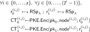
• $\mathsf {UFE.Enc}({\mathsf {mpk}},\mathsf {D})$ parses ${\mathsf {mpk}}$ as $(\mathsf {pk}_0,\mathsf {pk}_1,\mathsf {crs},\mathsf {H},(l_1,l_2,l_3))$ and appends to the memory data $\mathsf {D}$ the token-id 1, address 0 and the empty state $\epsilon$, encoded as bit-stings of length $l_1$, $l_2$ and $l_3$, respectively: $\mathsf {D}\leftarrow (\mathsf {D},1,0,\epsilon )$. (We assume from now on that $|\mathsf {D}|$ is a power of 2. This is without loss of generality since $\mathsf {D}$ can be padded.) $\mathsf {UFE.Enc}$ sets $\mathsf {z}{\leftarrow }\log (|\mathsf {D}|)$, samples a random string and constructs a perfectly balanced binary tree $\mathsf {T}:= \{\mathsf {node}^{(i,j)}\}$, where leafs are set as

  $$\begin{aligned} \forall j \in \{0,\ldots ,(|\mathsf {D}|-1)\}, \ \mathsf {node}^{(\mathsf {z},j)} \leftarrow (\mathsf {D}[j],\mathsf {tag},(\mathsf {z},j),0) \end{aligned}$$

  and intermediate nodes are computed as

  $$\begin{aligned} \forall i \in \&\{(\mathsf {z}-1),\ldots ,0\}, \ \forall j \in \{0,\ldots ,(2^i-1)\}, \\&\mathsf {node}^{(i,j)} \leftarrow (\mathsf {H}(\mathsf {node}^{(i+1,2j)},\mathsf {node}^{(i+1,2j+1)})). \end{aligned}$$

  $\mathsf {UFE.Enc}$ then encrypts each node independently under $\mathsf {pk}_0$ and $\mathsf {pk}_1$, i.e.

  

  and computes NIZK proofs that $\mathsf {CT}_0^{(i,j)}$ and $\mathsf {CT}_1^{(i,j)}$ encrypt the same content. More precisely,

  

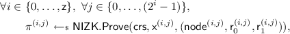
  where $\mathsf {x}^{(i,j)}$ is the NP statement

  $$ \exists (\mathsf {m},\mathsf {r}_0,\mathsf {r}_1): \mathsf {CT}_0^{(i,j)} = \mathsf {PKE.Enc}(\mathsf {pk}_0,\mathsf {m}; \mathsf {r}_0) \wedge \mathsf {CT}_1^{(i,j)} = \mathsf {PKE.Enc}(\mathsf {pk}_1,\mathsf {m}; \mathsf {r}_1). $$

  Finally, $\mathsf {UFE.Enc}$ lets

  $$ \mathsf {CT}:= \{(\mathsf {CT}_0^{(i,j)},\mathsf {CT}_1^{(i,j)},\pi ^{(i,j)})\}, $$

  which encodes a perfectly balanced tree, and outputs it as a ciphertext of memory data $\mathsf {D}$ under ${\mathsf {mpk}}$.

• $\mathsf {UFE.TokenGen}(\mathsf {msk},{\mathsf {mpk}},\mathsf {P},\mathsf {tid})$ parses $(\mathsf {pk}_0,\mathsf {pk}_1,\mathsf {crs},\mathsf {H},(l_1,l_2,l_3)) {\leftarrow }{\mathsf {mpk}}$, $(\mathcal {Q},\mathcal {T},\mathcal {Y},\delta ) {\leftarrow }\mathsf {P}$ and $\mathsf {sk}_0 {\leftarrow }\mathsf {msk}$. It then samples a new puncturable PRF key 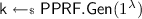. Next, it sets a circuit ${\widehat{\delta }}$ as described in Fig. 9, using the parsed values as the appropriate hardcoded constants with the same naming. $\mathsf {UFE.TokenGen}$ then obfuscates this circuit by computing . Finally, for simplicity in order to avoid having to explicitly deal with the data structure in the ciphertext, and following a similar approach as in [9], we define token $\mathsf {\overline{P}}$ not by its transition function, but by pseudocode, as the RAM program that executes on $\mathsf {CT}$ the following:

  • 1. Set initial state $\mathsf {st}{\leftarrow }\epsilon$, initial address $\mathsf {addr}{\leftarrow }0$ and empty output $\mathsf {y}{\leftarrow }\epsilon$.

  • 2. While $(\mathsf {y}= \epsilon )$

    • (a) Construct a tree $\overline{\mathsf {T}}$ by selecting from $\mathsf {CT}$ the leaf at address $\mathsf {addr}$ and the last $(l_1+l_2+l_3)$ leafs (that should encode $\mathsf {tid}$, $\mathsf {addr}$ and $\mathsf {st}$ if $\mathsf {CT}$ is valid), as well as all the necessary nodes to compute the hash values of their path up to the root.

    • (b) Evaluate $(\overline{\mathsf {T}},\mathsf {addr},\mathsf {y}) {\leftarrow }{\overline{\delta }}(\overline{\mathsf {T}})$.

    • (c) Update $\mathsf {CT}$ by writing the resulting $\overline{\mathsf {T}}$ to it.

  • 3. Output $\mathsf {y}$.

Fig. 9.

Specification of circuit ${\widehat{\delta }}$, as part of our updatable functional encryption scheme.

Theorem 1

Let $\mathsf {PKE}$ be an $\mathrm {IND}\text{- }\mathrm {CCA}$ secure public-key encryption scheme, let $\mathsf {NIZK}$ be a non-interactive zero knowledge proof system with perfect completeness, computational zero knowledge and statistical simulation soundness, let $\mathsf {H}$ be a collision-resistant hash function family, let $\mathsf {PPRF}$ be a puncturable pseudorandom function and let $\mathsf {Obf}$ be an iO-secure obfuscator that is also DI-secure w.r.t. the class of samplers described in $\mathrm {Game}_4$. Then, the updatable functional encryption scheme $\mathsf {UFE}[\mathsf {PKE},\mathsf {NIZK},\mathsf {H},\mathsf {PPRF},\mathsf {Obf}]$ detailed in Sect. 3.2 is selectively secure (as per definition in Fig. 8).

Proof

(Outline). The proof proceeds via a sequence of games as follows.

• $\mathrm {Game}_0$: This game is identical to the real $\mathrm {SEL}$ game when the challenge bit $b=0$, i.e. the challenger encrypts $\mathsf {D}_0$ in the challenge ciphertext.

• $\mathrm {Game}_1$: In this game, the common reference string and NIZK proofs are simulated. More precisely, at the beginning of the game, the challenger executes 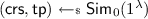to produce the $\mathsf {crs}$ that is included in the ${\mathsf {mpk}}$, and proofs in the challenge ciphertext are computed with $\mathsf {Sim}_1$ and $\mathsf {tp}$. The distance to the previous game can be bounded by the zero-knowledge property of $\mathsf {NIZK}$.

• $\mathrm {Game}_2$ : Let $\mathsf {T}_0 := \{\mathsf {node}^{(i,j)}_0\}$ be the perfectly balanced tree resulting from the encoding of $\mathsf {D}_0$ with $\mathsf {tag}_0$, and $\mathsf {T}_1 := \{\mathsf {node}^{(i,j)}_1\}$ the one resulting from the encoding of $\mathsf {D}_1$ with $\mathsf {tag}_1$, where $(\mathsf {D}_0,\mathsf {D}_1)$ are the challenge messages queried by the adversary and $(\mathsf {tag}_0,\mathsf {tag}_1)$ are independently sampled random tags. In this game, $\mathsf {CT}_1^{(i,j)}$ in the challenge ciphertext encrypts $\mathsf {node}^{(i,j)}_1$; the NIZK proofs are still simulated. This transition is negligible down to the $\mathrm {IND}\text{- }\mathrm {CPA}$ security of $\mathsf {PKE}$.

• $\mathrm {Game}_3$: In this game we hardwire a pre-computed lookup table to each circuit ${\widehat{\delta }}_l$, containing fixed inputs/outputs that allow to bypass the steps described in Fig. 9. If the input to the circuit is on the lookup table, it will immediately return the corresponding output. The lookup tables are computed such that executing the tokens in sequence starting on the challenge ciphertext will propagate the execution over $\mathsf {D}_0$ in the left branch and $\mathsf {D}_1$ in the right branch. Because the challenge ciphertext evolves over time as tokens are executed, to argue this game hop we must proceed by hardwiring one input/output at the time, as follows: (1) We hardwire the input/output of the regular execution [iO property of $\mathsf {Obf}$]; (2) we puncture the $\mathsf {PPRF}$ key of ${\widehat{\delta }}_l$ on the new hardwired input [functionality preservation under puncturing of $\mathsf {PPRF}$ + iO property of $\mathsf {Obf}$]; (3) we replace the pseudorandom coins used to produce the hardwired output with real random coins [pseudorandomness at punctured points of $\mathsf {PPRF}$]; (4) we use simulated NIZK proofs in the new hardwired output [zero-knowledge property of $\mathsf {NIZK}$]; (5) we compute circuit $\delta _l$ independently on the right branch before encrypting the hardwired output [$\mathrm {IND}\text{- }\mathrm {CPA}$ security of $\mathsf {PKE}$].

• $\mathrm {Game}_4$: In all circuits ${\widehat{\delta }}_l$, we switch the decryption key $\mathsf {sk}_0$ with $\mathsf {sk}_1$ and perform the operations based on the right branch, i.e. we modify the circuits such that $\mathsf {node}^{(i,j)} {\leftarrow }\mathsf {PKE.Dec}(\mathsf {sk}_1,\mathsf {CT}_1^{(i,j)})$. This hop can be upper-bounded by the distributional indistinguishability of $\mathsf {Obf}$. To show this, we construct an adversary $(\mathcal {S},\mathcal {B})$ against the DI game that runs adversary $\mathcal {A}$ as follows.

  Sampler $\mathcal {S}$ runs $\mathcal {A}_0$ to get the challenge messages $(\mathsf {D}_0,\mathsf {D}_1)$ and circuits $\delta _l$. Then, it produces the challenge ciphertext (same rules apply on $\mathrm {Game}_3$ and $\mathrm {Game}_4$), and compute circuits ${\widehat{\delta }}_l$ according to rules of $\mathrm {Game}_3$ (with decryption key $sk_0$) on one hand and according to rules of $\mathrm {Game}_4$ (with decryption key $\mathsf {sk}_1$) on the other. Finally, it outputs the two vectors of circuits and the challenge ciphertext as auxiliary information.

  Adversary $\mathcal {B}$ receives the obfuscated circuits ${\overline{\delta }}_l$ either containing $\mathsf {sk}_0$ or $\mathsf {sk}_1$ and the challenge ciphertext. With those, it runs adversary $\mathcal {A}_1$ perfectly simulating $\mathrm {Game}_3$ or $\mathrm {Game}_4$. $\mathcal {B}$ outputs whatever $\mathcal {A}_1$ outputs.

  It remains to show that sampler $\mathcal {S}$ is computationally unpredictable. Suppose there is a predictor $\mathrm {Pred}$ that finds a differing input for the circuits output by sampler $\mathcal {S}$. It must be because either the output contains a NIZK proof for a false statement (which contradicts the soundness property of $\mathsf {NIZK}$), or there is a collision in the Merkle tree (which contradicts the collision-resistance of $\mathsf {H}$), or the predictor was able to guess the random tag in one of the ciphertexts (which contradicts the $\mathrm {IND}\text{- }\mathrm {CCA}$ security of $\mathsf {PKE}$). Note that (1) the random tag is high-entropy, so lucky guesses can be discarded; (2) we cannot rely only on $\mathrm {IND}\text{- }\mathrm {CPA}$ security of $\mathsf {PKE}$ because we need the decryption oracle to check which random tag the predictor was able to guess to win the indistinguishability game against $\mathsf {PKE}$. We also rely on the fact that adversary $\mathcal {A}_0$ is legitimate in its own game, so the outputs in clear of the tokens are the same in $\mathrm {Game}_3$ and $\mathrm {Game}_4$.

• $\mathrm {Game}_5$: In this game, we remove the lookup tables introduced in $\mathrm {Game}_3$. We remove one input/output at the time, from the last input/output pair added to the first, following the reverse strategy of that introduced in $\mathrm {Game}_3$.

• $\mathrm {Game}_6$: Here, the challenge ciphertext is computed exclusively from $\mathsf {D}_1$ (with the same random tag on both branches). This transition is negligible down to the $\mathrm {IND}\text{- }\mathrm {CPA}$ security of $\mathsf {PKE}$.

• $\mathrm {Game}_7$: In this game, we move back to regular (non-simulated) NIZK proofs in the challenge ciphertext. The distance to the previous game can be bounded by the zero-knowledge property of $\mathsf {NIZK}$.

• $\mathrm {Game}_8$: We now switch back the decryption key to $\mathsf {sk}_0$ and perform the decryption operation on the left branch. Since $\mathsf {NIZK}$ is statistically sound, the circuits are functionally equivalent. We move from $\mathsf {sk}_1$ to $\mathsf {sk}_0$ one token at the time. This transition is down to the iO property of $\mathsf {Obf}$. This game is identical to the real $\mathrm {SEL}$ game when the challenge bit $b=1$, which concludes our proof.    $\square$

It is easy to check that the proposed scheme meets the correctness and efficiency properties as we defined in Sect. 3.1 for our primitive. The size of the ciphertext is proportional to the size of the cleartext. The size expansion of the token is however proportional to the number of steps of its execution, as the circuit ${\overline{\delta }}$ must be appropriately padded for the security proof.

4 Future Work

The problem at hand is quite challenging to realize even when taking strong cryptographic primitives as building blocks. Still, one might wish to strengthen the security model by allowing the adversary to obtain tokens adaptively, or by relaxing the legitimacy condition that imposes equal access patterns of extracted programs on left and right challenge messages using known results on Oblivious RAM. We view our construction as a starting point towards the realization of other updatable functional encryption schemes from milder forms of obfuscation.

References

Ananth, P., Boneh, D., Garg, S., Sahai, A., Zhandry, M.: Differing-inputs obfuscation and applications. IACR Cryptology ePrint Archive, Report 2013/689 (2013)
Arriaga, A., Barbosa, M., Farshim, P.: Private functional encryption: indistinguishability-based definitions and constructions from obfuscation. In: Dunkelman, O., Sanadhya, S.K. (eds.) INDOCRYPT 2016. LNCS, vol. 10095, pp. 227–247. Springer, Cham (2016). doi:10.1007/978-3-319-49890-4_13
Ananth, P., Sahai, A.: Functional encryption for turing machines. In: Kushilevitz, E., Malkin, T. (eds.) TCC 2016. LNCS, vol. 9562, pp. 125–153. Springer, Heidelberg (2016). doi:10.1007/978-3-662-49096-9_6
Bellare, M., Rogaway, P.: The security of triple encryption and a framework for code-based game-playing proofs. In: Vaudenay, S. (ed.) EUROCRYPT 2006. LNCS, vol. 4004, pp. 409–426. Springer, Heidelberg (2006). doi:10.1007/11761679_25
Bitansky, N., Canetti, R.: On strong simulation and composable point obfuscation. J. Cryptol. 27(2), 317–357 (2014)
Bellare, M., Hoang, V., Rogaway, P.: Foundations of garbled circuits. In: CCS 2012, pp. 784–796. ACM (2012)
Bellare, M., Stepanovs, I., Tessaro, S.: Contention in cryptoland: obfuscation, leakage and UCE. In: Kushilevitz, E., Malkin, T. (eds.) TCC 2016. LNCS, vol. 9563, pp. 542–564. Springer, Heidelberg (2016). doi:10.1007/978-3-662-49099-0_20
Boneh, D., Sahai, A., Waters, B.: Functional encryption: definitions and challenges. In: Ishai, Y. (ed.) TCC 2011. LNCS, vol. 6597, pp. 253–273. Springer, Heidelberg (2011). doi:10.1007/978-3-642-19571-6_16
Canetti, R., Chen, Y., Holmgren, J., Raykova, M.: Succinct adaptive garbled RAM. IACR Cryptology ePrint Archive, Report 2015/1074 (2015)
Canetti, R., Holmgren, J.: Fully succinct garbled RAM. In: ITCS 2016, pp. 169–178. ACM (2016)
Canetti, R., Holmgren, J., Jain, A., Vaikuntanathan, V.: Indistinguishability obfuscation of iterated circuits and RAM programs. IACR Cryptology ePrint Archive, Report 2014/769 (2014)
Canetti, R., Holmgren, J., Jain, A., Vaikuntanathan, V.: Succinct garbling and indistinguishability obfuscation for RAM programs. In: STOC 2015, pp. 429–437. ACM (2015)
Desmedt, Y., Iovino, V., Persiano, G., Visconti, I.: Controlled homomorphic encryption: definition and construction. IACR Cryptology ePrint Archive, Report 2014/989 (2014)
Garg, S., Gentry, C., Halevi, S., Raykova, M., Sahai, A., Waters, B.: Candidate indistinguishability obfuscation and functional encryption for all circuits. In: FOCS 2013, pp. 40–49. IEEE Computer Society (2013)
Gentry, C., Halevi, S., Lu, S., Ostrovsky, R., Raykova, M., Wichs, D.: Garbled RAM revisited. In: Nguyen, P.Q., Oswald, E. (eds.) EUROCRYPT 2014. LNCS, vol. 8441, pp. 405–422. Springer, Heidelberg (2014). doi:10.1007/978-3-642-55220-5_23
Gentry, C., Halevi, S., Raykova, M., Wichs, D.: Outsourcing private RAM computation. In: FOCS 2014, pp. 404–4013. IEEE Computer Society (2014)
Goyal, V., Jain, A., Koppula, V., Sahai, A.: Functional encryption for randomized functionalities. In: Dodis, Y., Nielsen, J.B. (eds.) TCC 2015. LNCS, vol. 9015, pp. 325–351. Springer, Heidelberg (2015). doi:10.1007/978-3-662-46497-7_13
Ishai, Y., Pandey, O., Sahai, A.: Public-coin differing-inputs obfuscation and its applications. In: Dodis, Y., Nielsen, J.B. (eds.) TCC 2015. LNCS, vol. 9015, pp. 668–697. Springer, Heidelberg (2015). doi:10.1007/978-3-662-46497-7_26
Lu, S., Ostrovsky, R.: How to garble RAM programs? In: Johansson, T., Nguyen, P.Q. (eds.) EUROCRYPT 2013. LNCS, vol. 7881, pp. 719–734. Springer, Heidelberg (2013). doi:10.1007/978-3-642-38348-9_42
Naor, M., Yung, M.: Public-key cryptosystems provably secure against chosen ciphertext attacks. In: STOC 1990, pp. 427–437. ACM (1990)
O’Neill, A.: Definitional issues in functional encryption. IACR Cryptology ePrint Archive, Report 2010/556 (2010)
Sahai, A., Waters, B.: How to use indistinguishability obfuscation: deniable encryption, and more. In: STOC 2014, pp. 475–484. ACM (2014)
Yao, A.: How to generate and exchange secrets. In: FOCS 1986, pp. 162–167. IEEE Computer Society (1986)
Acknowledgements
The authors would like to thank Karol Zebrowski for his contribution to an earlier version of this work. Afonso Arriaga is supported by the National Research Fund, Luxembourg, under AFR Grant No. 5107187, and by the Doctoral School of Computer Science & Computer Engineering of the University of Luxembourg. Vincenzo Iovino is supported by the National Research Fund, Luxembourg. Qiang Tang is supported by a CORE (junior track) grant from the National Research Fund, Luxembourg.
Author information
Authors and Affiliations
Corresponding author
Editor information
Editors and Affiliations
Rights and permissions
Copyright information
© 2017 Springer International Publishing AG
About this paper
Cite this paper
Arriaga, A., Iovino, V., Tang, Q. (2017). Updatable Functional Encryption. In: Phan, RW., Yung, M. (eds) Paradigms in Cryptology – Mycrypt 2016. Malicious and Exploratory Cryptology. Mycrypt 2016. Lecture Notes in Computer Science(), vol 10311. Springer, Cham. https://doi.org/10.1007/978-3-319-61273-7_17
Download citation
DOI: https://doi.org/10.1007/978-3-319-61273-7_17
Published:
Publisher Name: Springer, Cham
Print ISBN: 978-3-319-61272-0
Online ISBN: 978-3-319-61273-7
eBook Packages: Computer ScienceComputer Science (R0)