
Abstract
Process mining is an emerging area that synergically combines model-based and data-oriented analysis techniques to obtain useful insights on how business processes are executed within an organization. Through process mining, decision makers can discover process models from data, compare expected and actual behaviors, and enrich models with key information about their actual execution. To be applicable, process mining techniques require the input data to be explicitly structured in the form of an event log, which lists when and by whom different case objects (i.e., process instances) have been subject to the execution of tasks. Unfortunately, in many real world set-ups, such event logs are not explicitly given, but are instead implicitly represented in legacy information systems. To apply process mining in this widespread setting, there is a pressing need for techniques able to support various process stakeholders in data preparation and log extraction from legacy information systems. The purpose of this paper is to single out this challenging, open issue, and didactically introduce how techniques from intelligent data management, and in particular ontology-based data access, provide a viable solution with a solid theoretical basis.
Access provided by CONRICYT-eBooks. Download chapter PDF
Keywords
1 Introduction
SMEsFootnote 1 and large enterprises are increasingly adopting business process management to continuously optimise internal work, achieve its strategic business objectives, and guarantee quality of service to their customers. Business process management provides methods, techniques, and tools to comprehensively support managers and domain experts in the design, administration, configuration, execution, monitoring, and analysis of operational business processes [1]. As pointed out in [2], a business process consists of a set of activities that are performed in coordination in an organisational and technical environment, and that jointly realise a business goal. At execution time, the process is instantiated multiple times, leading to different sequences of activity executions performed by different resources, where each sequence refers to the evolution of a main, so-called case object. The instantiation of each activity on a case, in turn, gives raise to multiple events, indicating the evolution of each activity instance from its start to its completion or cancellation, according to a so-called activity transactional lifecycle.
The notion of case depends on the nature of the process, and on the perspective taken to understand the process. For example, in an order-to-cash scenario, the case typically corresponds to the order first issued by a customer, then manipulated within the enterprise, paid by the customer, and finally shipped to her. Different orders give raise to different process instances and corresponding execution traces. While using the order as a case object to understand the process is the most natural choice in this scenario, alternative case objects may be useful to understand the same process from different viewpoints. For example, suppose that the enterprise managing orders relies on an external shipping company to handle the order deliveries. Such a shipping company may prefer to consider its couriers as cases, and consequently focus its attention to the flow of operations performed by each courier, possibly involving multiple orders at once.
Classical BPM is purely model-driven: processes are elicited using human ingenuity through interviews with the involved stakeholders, and then used in a prescriptive manner to orchestrate the process execution, and to indicate to such stakeholders how they are expected to behave. This has been increasingly considered as the main limiting factor towards large-scale adoption of BPM. On the one hand, people tend to consider processes not as a support, but as a form of control over their behaviour. This is especially true in so-called knowledge-intensive settings, where it is not possible to foresee all potential state of affairs in advance, nor to enumerate all possible courses of execution, which have in fact to be adaptively and incrementally devised at runtime by the involved stakeholders, leveraging their own knowledge. On the other hand, there is an intrinsic mismatch between processes as reflected in models, and process executions resulting from the actual progression of cases in a real organisational setting. Even when processes are executed in line with the elicited process models, considering execution data is crucial to understand how work is effectively carried out inside the enterprise, and consequently obtain useful insights related to key performance indicators (such as average completion time for cases), the detection of bottlenecks and of working relationships among persons, and the identification of frequent and infrequent behaviours, to name a few.
To resolve this mismatch between process models and process executions, the emerging area of process mining [3, 4] has become increasingly popular both in the academia and the industry. Process mining is a collection of techniques that combine, in a synergic way, model-based and data-oriented analysis to obtain useful insights on how business processes are executed in a real organisational environment. Through process mining, decision makers can discover process models from data, compare expected and actual behaviours, and enrich models with information obtained from their execution. The process mining manifesto [3] provides a thorough introduction to process mining. The book by van der Aalst [4] is the main reference material for students, researchers and professionals interested in this field. In addition, a list of successful stories related to the application of process mining to concrete case studies can be found at the web page of IEEE CIS Task Force on Process MiningFootnote 2.
The applicability of process mining depends on two crucial factors:
-
the availability of high-quality event data, and of event logs containing correct and complete event data about which cases have been executed, which events occurred for each case, and when they did occur;
-
the representation of such data in a format that is understandable by process mining algorithms, such as the XML-based, IEEE standard eXtensible Event Stream (XES) [5].
Event data structured in this form are only readily available if the enterprise under analysis adopts a business process management system, providing direct support for orchestrating the execution of cases according to a given process model, and at the same time providing logging capabilities for cases, events, and corresponding attributes. In this setting, the extraction of an event log for process mining is quite direct. Unfortunately, in many real world settings, the enterprise exploits functionalities offered by more general enterprise systems such as ERPFootnote 3, CRMFootnote 4, SCMFootnote 5, and other business suites. In addition, such systems are typically configured for the specific needs of the company, and connected to domain-specific and other legacy information systems. Within such complex systems, event logs are not explicitly present, but have instead to be reconstructed by extracting and integrating information present in all such different, possibly heterogeneous data sources.
To apply process mining in this widespread setting, there is a pressing need for techniques that are able to support data and process analysts in the data preparation phase [3], and in particular in the extraction of event data from legacy information systems. The purpose of this paper is to single out this challenging, open issue, and didactically introduce how techniques from intelligent data management, and in particular ontology-based data access (OBDA) [6,7,8], provide a viable solution with a solid theoretical basis. The resulting approach, called onprom [9], comes with a methodology supporting data and process analysts in the conceptual identification of event data, answering questions like: (i) Which are relevant concepts and relations? (ii) How do such concepts/relations map to the underlying information system? (iii) Which concepts/relations relate to the notion of case, event, and event attributes? The methodology is backed up by a toolchain that, once the aforementioned questions are answered, automatically extracts an event log conforming to the chosen perspective, and obtained by inspecting the data where they are, thanks to the OBDA paradigm and tools.
2 Process Mining: A Gentle Introduction
In this section, we give broad introduction to process mining, starting with the reference framework for process mining, the main process mining techniques, and an excursus of some contemporary process mining tools. In the second part of the section, we focus on the data preparation phase for process mining, recalling the notion of event log and of the event log format expected by process mining algorithms.

The reference framework for process mining, and the three types of process mining techniques: discovery, conformance, and enhancement [3]
2.1 The Process Mining Framework
The reference framework for process mining is depicted in Fig. 1. On the one hand, process mining considers conceptual models describing processes, organisational structures, and the corresponding relevant data. On the other hand, it focuses on the real execution of processes, as reflected by the footprint of reality logged and stored by the software systems in use within the enterprise. For process mining to be applicable, such information has to be structured in the form of explicit event logs. In fact, all process mining techniques assume that it is possible to record the sequencing of relevant events occurred within the enterprise, such that each event refers to an activity (i.e., a well-defined step in some process) and is related to a particular case [3]. Events may have additional information stored in event logs. In fact, whenever possible, process mining techniques use extra information such as the exact timestamp at which the event has been recorded, the resource (i.e., person or device) that generated the event, the event type in the context of the activity transactional lifecycle (e.g., whether the activity has been started, cancelled, or completed), the timestamp of the event, or data elements recorded with the event (e.g., the size of an order).

The process for managing papers in a simplified conference submission system; gray tasks are external to the conference information system and cannot be logged.
Example 1
As a running example, we consider a simplified conference submission system, which we call ConfSys. The main purpose of ConfSys is to coordinate authors, reviewers, and conference chairs in the submission of papers to conferences, the consequent review process, and the final decision about paper acceptance or rejection. Figure 2 shows the process control flow considering papers as case objects. Under this perspective, the management of a single paper evolves through the following execution steps. First, the paper is created by one of its authors, and submitted to a conference available in the system. Once the paper is submitted, the review phase for that paper starts. This phase of the process consists of a so-called multi-instance section, i.e., a section of the process where the same set of activities is instantiated multiple times on the same paper, and then executed in parallel. In the case of ConfSys, this section is instantiated for each reviewer selected by the conference chair for the paper, and consists of the following three activities: (i) a reviewer is assigned to the paper; (ii) the reviewer produces the review; (iii) the reviewer submits the review to ConfSys. The multi-instance section is considered completed only when all its parallel instantiations are completed. Hence the process continues as soon as all appointed reviewers have submitted their review. Based on the submitted reviews, the chair then decides if the paper has to be accepted or rejected. In the former case, one of the authors is expected to upload the final (camera ready) version of the paper, addressing the comments issued by reviewers.
It is important to notice, again, that the process model shown in Fig. 2 is only one of the several representations of the process, reflecting the perspective of papers as process cases. A completely different model would emerge from the same process, when focusing on the evolution of reviews instead of that of papers.
A fragment of a sample event log tracking the evolution of papers within ConfSys is shown in Table 1. The logged activities corresponds to those activities in Fig. 2 that actually comprise interaction with the software system of ConfSys, together with those activities that are autonomously executed by the system itself. From the point of view of the software system, the former activities are called human-interaction activities, and the latter are called system activities. These two types of activity contrast with purely human activities, which are executed by humans in the concrete world without software support, and can be indirectly logged only if accompanied by corresponding human-interaction activities. An example of this can be seen in Fig. 2, where review paper is a purely human activity carried out by a reviewer without the intervention of the software system, and is in fact coupled with submit review, a human-interaction activity executed by a reviewer to communicate to ConfSys the outcome of review paper. As we can see from the table there are two different cases (i.e., papers), with various events, each involving different responsible actors. Both cases regard papers that have been subject only to a single review, but in the first case the paper is accepted, while in the second one it is rejected. 
How do process mining techniques exploit models and/or event logs to extract useful insights, and what do they offer concretely? The three main types of process mining techniques are marked by the three, thick red arrows in the bottom part of Fig. 1. We briefly discuss them next.
Discovery starts from an event log and automatically produces a process model that explains the different behaviours observed in the log, without assuming any prior knowledge on the process. The vast majority of process discovery algorithms focus on the discovery of the process control-flow, towards generating a model that indicates what are the allowed sequences of activities according to the log. One of the first algorithms in this line is the \(\alpha \) algorithm [10], which produces a Petri net that compactly explains the sequences of activities present in a given event log. Contemporary control-flow discovery algorithms are much more sophisticated and richer in terms of the produced results, and differ from each other along several dimensions, such as the concrete language they use for the discovered model, the ability of enriching control-flow with additional elements (such as decision and data logic), and the ability of incorporating multiple abstraction levels (i.e., to hide/show details about infrequent or outlier behaviours). In addition, their quality depends on how they trade between the four crucial factors of:
-
1.
fitness - to what extent the produced model correctly reconstructs the behaviours present in the log;
-
2.
simplicity - how much is the produced model understandable to humans;
-
3.
precision - how much is the produced model adherent to the behaviours contained in the log;
-
4.
generalisation - what is the extent of behaviours not contained in the log, but supported by the model.
In addition to the control-flow perspective, many other aspects are addressed by process discovery techniques (cf. Sect. 2.2). For example, a class of discovery algorithms focuses on process resources, producing a social network that explains the hand-over of work among the stakeholders involved in the process. This is only possible if the input event log contains resource-related information (this is, e.g., the case of the log shown in Table 1).
Conformance Checking compares an existing process model and an event log for the same process, with the aim of understanding the presence and nature of deviations. Conformance checking techniques take as input an event log and a (possibly discovered) process model, and return indications related to the adherence of the behaviours contained in the log to the prescriptions contained in the model. Detected deviations provide on the one hand the basis to take countermeasures on non-conforming behaviours, and on the other hand to act on the considered model and suitable re-engineer it so as to incorporate also the unaligned behaviours. In this light, conformance checking ranges from the detection and localisation of sources of non-conformance, to the estimation of their severity, the computation of conformance metrics summarising them, and possibly even their explanation and diagnosis.
Enhancement improves an existing process model using information recorded inside an event log for that process. The input of enhancement techniques is a process model and an event log, and the output is a new process model that incorporates and reflects new information extracted from the data. The first important class of enhancement techniques is that of extension, where the input process model is not altered in its structure, but is extended with additional perspectives, using information present in the log. Examples of extension techniques are those that incorporate frequency- and time-related information into the process model, using the timestamps and the frequencies about activity executions present in the log. The extended process model provides an immediate feedback about which parts of the process are most exploited and which contain outlier behaviours, as well as where bottlenecks are located. A second important class of enhancement techniques is that of repair, where deviations detected by checking the conformance of the input event log to the input process model are resolved by suitably modifying the process model. For example, if two activities are sequentially ordered in the given process model, but according to the log they may appear in any order, then the process model may be evolved by relaxing the sequence, and allowing for their concurrent execution.
Example 2
Figure 3 shows the result of a control-flow discovery algorithm, applied to an event log from ConfSys whose structure obeys to what reported in Table 1. Notably, the algorithm does not only discover the control-flow of a process model explaining the behaviours contained in the log, but also extends such a model with frequency information, colouring activities and setting the width of sequence flow connectors depending on how frequent they are. 

2.2 Application of Process Mining
Since process mining is a relatively new field, methodologies supporting data and process analysts in the application of process mining techniques are still in their infancy [12]. In general, five main stages are foreseen for process mining projects. The first phase concerns planning and justification of the project, formulating which research questions shall be answered through process mining, and defining the boundaries of the analysis. This includes the definition of which perspective has to be taken for the analysis, including which notion(s) of case object to consider.
The second phase substantiates the first one by handling the extraction of the relevant event data from the software systems of he enterprise. As argued in the introduction, this phase is in general extremely challenging, and for the most part still based on manual, ad-hoc extraction procedures.
The third phase exploits control-flow process discovery techniques towards the construction of a first, process model explaining the behaviours reflected in the extracted data, and deriving which are the allowed orderings of activities. The resulting model is usually represented using formal languages such as variants of Petri nets, or concrete control-flow modelling notations such as BPMN, EPCs, or UML activity diagrams. The so-obtained model can be enhanced with information present in the log.
The fourth phase consists in the incorporation of additional dimensions, so as to obtain integrated models simultaneously accounting for multiple perspectives, like the organisational perspective (i.e., the actors, roles, groups/departments are involved in the process execution), the case perspective (i.e., relevant data elements that are attached to cases), and the time perspective (i.e., execution times, durations, latencies, and frequencies information about the execution of activities and/or the execution of a certain route within the process). Even though these different perspectives are non-exhaustive and partly overlapping, they provide a quite comprehensive overview of the aspects that process mining aims to analyse [4].
The fifth phase aims at exploiting the results obtained so far so as to produce insightful indications, suggestions, recommendations, and predictions on running and future cases, i.e., to provide operational decision support to decision makers and to the people involved in the actual execution of the process under study.
2.3 Process Mining Tools
A plethora of process mining techniques and technologies have been developed and successfully employed in several application domainsFootnote 6. We provide here a non-exhaustive list of contemporary process mining solutions.
-
ProM (Process Mining framework)Footnote 7 is an Open Source framework for process mining algorithms [13], based on JAVA. It provides a plug-in based, integration platform [14] that users and developers of process mining can exploit to deploy and run their techniques. This pluggable architecture currently hosts a huge amount of plug-ins covering all the different aspects of process mining, from data import to discovery, conformance checking, enhancement along different perspectives [4]. Hence, it enable users to apply the latest developments in process mining research on their own data. Finally, RapidProMFootnote 8 [15] is an extension of RapidMiner based on ProM that supports users in pipelining different ProM plug-ins based on the paradigm of scientific workflows.
-
Celonis Footnote 9 is a commercial, widely adopted process mining software that support various file formats and database management systems to load event data. Its distinctive feature is the possibility of applying process mining natively on top of enterprise systems like SAP. In addition, it exploits well-assessed data warehousing (OLAP) techniques to store and process event data [4].
-
Disco Footnote 10 is a commercial, stand-alone and lightweight process mining tool. It supports various file formats as input, in particular providing native support for importing CSV files, which can be annotated with case and event information prior to the import. Disco has usability, fidelity, and performance as design priorities, and makes process mining easy and fast [16].
-
ARIS PPM Footnote 11 is a tool that can be used to automatically assess business processes and their execution data in terms of speed, cost, quality and quantity, at the same time identifying optimisation opportunities. It ranges from analysis of historical data to process discovery, and notably provides dedicated techniques for the analysis of the organisational structure and improving collaboration.
Beside the aforementioned solutions, worth mentioning are non-commercial tools such as PMLABFootnote 12 and CoBeFraFootnote 13, as well as commercial tools such as Enterprise Discovery SuiteFootnote 14, Interstage Business Process Manager AnalyticsFootnote 15, MinitFootnote 16, myInvenioFootnote 17, RialtoFootnote 18, Perceptive Process MiningFootnote 19, QPR ProcessAnalyzerFootnote 20, and SNP Business Process AnalysisFootnote 21.

An example of XES event log
2.4 The XES Standard
As extensively argued before, the application of process mining techniques requires the input data to be structured in a format where key notions like case objects and events are explicitly represented, and where their corresponding data are structured in a way that lends itself to be automatically processed. This fundamental requirements led to the development of standard formats for the representation and storage of event data for process mining. In recent years, the XES (eXtensible Event Stream) format emerged as the main reference format for the storage, interchange, and analysis of event logs. XES appeared for the first time in 2009 [17], as the successor of the MXML format [18]. It quickly became the de-facto standard in this area, adopted by the IEEE Task Force on Process MiningFootnote 22, eventually becoming an official IEEE standard in 2016 [5].
XES is based on XML, and adopts an extensible paradigm that only fixes a minimal structure for event data, allowing one to enrich it with domain-specific attributes and features. More specifically, an XES event log document is an XML document formed by the following core components: (i) log, (ii) trace, (iii) event, (iv) attribute, (v) global attribute, (vi) classifier, and (vii) extension. We briefly review each such components in the remainder of this section, referring the interested reader to the official IEEE XES standard for further details. Figure 4 encodes in XES a portion of the event log from Table 1.
Log is the root component in XES. It aggregates information about the logged evolution of multiple cases for a process. In the XML serialisation of XES, it is encoded using the XML element  , which comes with two mandatory attributes:
-
xes.version, indicating which version of the standard is used;
-
xes.features, declaring which features of the standard are employed (if none, then it has an empty string as value).
Example 3
The following code

is an example of XES log declaration, which indicates that the version 2.0 of the standard is used, relying on nested attributes. 
Trace corresponds to the execution log of a single case, in turn comprising a sequence of events that occurred for that case. In our ConfSys running example, a trace may consist of all logged events for a paper, a review, or a user, depending on the adopted notion of case. In the XML representation of XES, a trace is encoded using the XML element  , and does not have any attribute. A trace element is directly contained within the log root element, and consequently each trace belongs to a log, whereas each log contains possibly many traces.
Event represents the occurrence of a relevant atomic execution step for a specific case. Usually, this corresponds to the (completion of) execution of an activity instance, or to the progression of an activity instance within its transactional lifecycle, but this is not mandatorily prescribed by the standard.
In the XML serialisation of XES, this component is encoded using the XML tag  , and does not have any attribute. An event element is contained within the trace element corresponding to its target case, and consequently each event belongs to a trace, whereas each trace contains in general many events.
Attributes represent relevant information items associated to a log, trace, or event. Each attribute element is then child of one of such elements, which in turn may contain in general many attributes. The concrete representation of an attribute follows the typical key-value patterns, where the key describes the type of information slot, while the value is the information stored inside such a slot. The value, in turn, may be primitive, a collection, or a complex structure containing other attributes, consequently giving raise to elementary, composite, and nested attributes.
An elementary attribute is an attribute that has an single value. The XES standard supports several types of elementary attributes, namely: (i) string, (ii) datetime, (iii) integer, (iv) real number, (v) boolean, and (vi) ID. In the XML serialisation of XES, an elementary attribute is encoded using the XML tag that corresponds to its type. For instance, the XML tag  encodes an elementary attribute of type “string”. This XML element also mandatorily comes with two XML attributes key and value, respectively capturing the name of the key and the value carried by the attribute.
Example 4
The following XML element

declares an attribute of type string in XES, indicating its key and value. 
A composite attribute is an attribute that may contain several values. In XES 2.0 [19], there are two kinds of composite attributes, namely list and container, respectively addressing ordered and unordered collections. However, in the official IEEE XES standard [5], only lists are provided. Based on [5], the list attribute is represented as an XML element  , with key as mandatory attribute. The values belonging to the list are in turn represented as attributes element enclosed within a
  element, direct child of the
  element.
Example 5
The XML element

represents a XES composite attribute containing two elementary attributes, respectively representing the main and delivery address for an expedition. 
Global attributes are used to define a “template” for attributes to be attached to each element of a certain kind within the given XES document. This makes it possible to declare recurrent attributes that will be consistently attached to each trace or event contained in the log. According to the official IEEE XES Standard [5], global attributes are declared within the root,  element, as elements called
  coming with a scope XML attribute that defines the selected target element kind (trace, or event). Inside such an element, a set of (global) attributes are defined using the standard structure, with the key semantical difference that the value represents, in this context, the default value taken by the attribute once it is attached to a target element.
Example 6
The following excerpt of an XES document

declares different global attributes. The first  element declares that each trace contained in the log will come with a string attribute with key concept:name having a value that, unless specified, will be the string MyTrace. The second
  element targets instead events, and declares that each event element contained in the log will come with three attributes respectively representing the event execution time, the type of event within the activity transactional lifecycle, and the name of the corresponding activity (with their respective default values).
Classifiers are used to provide identification schemes for the elements in a log, based on a combination of attributes associated to them. Similarly to the case of global attributes, each classifier comes with a scope defining whether the classifier is applied to traces or events, and with a combination of strings that represent keys of global attributes attached to the same scope. An event (resp., trace) classifier mentioning strings \(k_1,\ldots ,k_n\), which are keys of global attributes with scope “event” (resp., “trace”), states that the identity of events (resp., traces) is defined by the values associated to such keys, i.e., that two events (resp., traces) are identical if and only if they assign the same values to the attributes characterised by those keys.
The declaration of a classifier is done in the XML serialisation of XES by inserting a  element as child of
  , providing an attribute called scope whose value denotes whether the scope is that of event or trace, and an attribute called keys whose value is a comma-separated set of strings pointing to keys of global attributes defined over the same scope.
Example 7
Consider the following excerpt of an XES document:

It indicates that the global attribute with key concept:name provides an identification scheme for events. 
Extensions capture pre-defined sets of global attributes with a clear semantics. In fact, the XES standard allows the modeller to introduce arbitrary domain-specific attributes, whose meaning may be ambiguous and difficult to interpret by other humans or third-party algorithms. The notion of extension fixes this issue by providing a mechanism to define a set of pre-defined attribute keys together with a reference to documentation that describes their meaning. Specifically, each extension must have a name, a prefix and a Uniform Resource Identifier (URI). The prefix is used to unambiguously contextualise the attribute keys and avoid name clashes, whereas the URI to the definition of the extension. An XES event log making use of a particular extension must declare it at the level of its  element. Notably, the official IEEE XES standard comes with a set of common extensions defining attributes to capture domain-independent important aspects such as: 1. (name of the) activity to which an event refers; 2. timestamp information about the actual time at which the event has been recorded; 3. resource information describing the resource that generated the event; 4. information about the type of event in terms of a corresponding transition within a standard transactional lifecycle for activities, also described in the standard itself.
Example 8
The following excerpt of an XES event log

declares that the time extension is employed in the log, and that the definition for such an extension may be found at the provided URI. The timestamp attribute, defined in the time extension, is then used in the definition of an event, so as to indicate when such an event has been recorded. 
2.5 The Data Preparation Phase
Thanks to the IEEE XES standard (cf. Sect. 2.4), the challenging phase of data preparation for process mining (i.e., the second phase in the description provided in Sect. 2.2) now has a clear target: it amounts to analyse the event data as natively stored by an enterprise, and to consequently devise suitable mechanisms to extract those data and encode them in the form of an XES log. This phase is extremely delicate because insightful process mining results cannot be obtained if the starting data miss important information or do not reflect the boundaries and research questions and defined in during the first phase of any process mining project. The complexity, and the availability of tool support, to extract event logs from the native enterprise logs depends on several factors, related to the quality, comprehensiveness, and structure of such data. The process mining manifesto provides an intuitive set of criteria to assess the maturity of enterprise logs, which in turn characterise the difficulty of extracting event logs. Specifically, five maturity levels are introduced:
-
 enterprise logs are low-quality logs that are usually filled in manually, and that include false positives and false negatives, i.e., contain events that do not correspond to reality, while miss events that occurred.
 -
 enterprise logs are automatically recorded by generic software systems that can be circumvented by their users, and that are consequently incomplete, at the same time possibly containing improperly recorded events.
 -
 enterprise logs are trustworthy, but possibly incomplete logs automatically recorded through reliable software systems but without following a systematic approach.
 -
 enterprise logs are high-quality, trustworthy and complete logs, recorded systematically by software systems where the key notions of cases and activities are represented explicitly;
 -
 enterprise logs are top-quality logs, where events are recorded in a systematic, comprehensive, and reliable manner, and where all event data have a shared, well-defined unambiguous semantics.
 enterprise logs are low-quality logs that are usually filled in manually, and that include false positives and false negatives, i.e., contain events that do not correspond to reality, while miss events that occurred.
 enterprise logs are automatically recorded by generic software systems that can be circumvented by their users, and that are consequently incomplete, at the same time possibly containing improperly recorded events.
 enterprise logs are trustworthy, but possibly incomplete logs automatically recorded through reliable software systems but without following a systematic approach.
 enterprise logs are high-quality, trustworthy and complete logs, recorded systematically by software systems where the key notions of cases and activities are represented explicitly;
 enterprise logs are top-quality logs, where events are recorded in a systematic, comprehensive, and reliable manner, and where all event data have a shared, well-defined unambiguous semantics.
The literature abounds of techniques and tools to handle the extraction of event logs from  and
and  enterprise logs, which are typically generated by BPM/workflow management systems. For example, academic efforts such as ProMimport [20] and XESame [13] provides support in the extraction of MXML/XES event logs from relational databases that contain explicit information about cases, activities, events, and their timestamps. Commercial tools like Disco, Celonis, and Minit, allows users to import CSV files, and guide them in annotating the columns contained therein with such key notions.
However, much less support is provided to users interested in the application of process mining starting from  enterprise logs. Such logs are widespread in reality, as they correspond to data stored by widely adopted enterprise systems such as ERP, CRM, and SCM solutions, as well as data generated by trustworthy, domain-specific legacy information systems. This is why the typical approach followed in this case is to devise ad-hoc, Extract, Transform, and Load (ETL) procedures. Such procedures need to be manually instrumented, assuming a fixed perspective on the data, and covering the following three steps [4]:
-
1.
extraction of data from the native enterprise systems, according to the chosen perspective;
-
2.
transformation of the extracted data, dealing with syntactical and semantical issues, towards fitting the operational needs;
-
3.
load of data into a target system (such as a data warehouse or a dedicated relational database), from which a corresponding XES log can be extracted directly.
This procedure is not only inherently difficult and error prone, but does not lend itself to incrementally and iteratively analyse the enterprise data according to different perspectives (e.g., different boundaries for the analysis, and/or multiple notions of case). In fact, every time the perspective and/or the scope of the analysis changes, an entirely new ETL-like set up has to be instrumented [9]. After having introduced the paradigm of Ontology-Based Data Access in Sect. 3, we show how in Sect. 4 how such a paradigm can be exploited to better support data and process analysts in the extraction of event logs from  enterprise data.
3 Ontology-Based Data Access
Ontologies are used to provide the conceptualization of a domain of interest, and mechanisms for reasoning about it. The standard language for representing ontologies is the Web Ontology Language (OWL 2), which has been standardized (in its second edition) by the W3C [21]. The formal foundations for ontologies, and in particular for OWL 2, are provided by Description Logics (DLs) [22], which are logics specifically designed to represent structured knowledge and to reason upon it.
In DLs, the domain to represent is structured into classes of objects of interest that have properties in common, and these properties are explicitly represented through relevant relationships that hold among the classes. Concepts denote classes of objects, and roles denote (typically binary) relations between objects. Both are constructed, starting from atomic concepts and roles, by making use of various constructs, and the set of allowed constructs characterizes a specific DL. The knowledge about the domain is then represented by means of a DL ontology, where a separation is made between general structural knowledge and specific extensional knowledge about individual objects. The structural knowledge is provided in a so-called TBox (for “Terminological Box”), which consists of a set of universally quantified assertions that state general properties about concepts and roles. The extensional knowledge is represented in an ABox (for “Assertional Box”), consisting of assertions on individual objects that state the membership of an individual in a concept, or the fact that two individuals are related by a role.
The setting we are interested in here, however, is the one in which the extensional information, i.e., the data, is not maintained as an ABox, but is stored in an information system, represented as a relational data sourceFootnote 23, and the TBox of the ontology is used not only to capture relevant structural properties of the domain, but also acts as a conceptual data schema that provides a high-level view over the data in the information system. In other words, users formulate their information requests in terms of the conceptual schema provided by the TBox of the ontology, and use it to access the underlying data source. The connection between the conceptual schema/TBox and the information system is provided by a declarative mapping specification. Such specification is used to translate the user requests, i.e., the queries the user poses over the conceptual schema, into queries to the information system, which can then directly be answered by the corresponding relational database engine. This setting is known as ontology-based data access (OBDA) [6, 7], and we are describing it more in detail below.
3.1 Lightweight Ontology Languages
An important aspect to note in the OBDA setting outlined above, is that the data source is in general a full-fledged relational database, and therefore it might be very large (especially when compared to the size of the TBox). On the other hand, the user queries formulated over the TBox, have to be answered while fully taking into account the domain semantics encoded in the TBox itself, i.e., in general under incomplete information. This means that query answering does not correspond to query evaluation, but amounts to a form of logical inference, which in general is inherently more complex than query evaluation [23]. More specifically, the complexity of query evaluation strongly depends on the form of the TBox (according to the usual tradeoff between expressive power and efficiency of inference). Therefore we need to carefully choose the language in which the TBox is expressed, so as to guarantee that query answering can be done efficiently, in particular in data complexity, i.e., when the complexity is measured with respect to the size of the data only [24]. Ideally, we would like to fully take into account the constraints encoded in the TBox, and at the same time delegate query evaluation over the data source to the relational DBMS in which the data is stored, so as to leverage the more than 30 years of experience gained with commercial relational technology.
We present now a so-called lightweight ontology language, specifically, \(\textit{DL-Lite}_{\mathcal {{A}}}\) of the DL-Lite family, which is a family of DLs that have been carefully designed so as to allow for efficient query answering over the TBox by relying on standard SQL query evaluation done by a relational DBMS [6, 25, 26]. The logics of the DL-Lite family (and specifically, the \(\textit{DL-Lite}_{\mathcal {{R}}}\) sub-language of \(\textit{DL-Lite}_{\mathcal {{A}}}\)) provide the basis for OWL 2 QL, one of the three standard profiles (i.e., sub-languages) of OWL 2 [21, 27], which has been specifically designed to capture the essential features of conceptual modeling formalisms (see also Sect. 3.2). In line with what available in OWL 2 and OWL 2 QL, \(\textit{DL-Lite}_{\mathcal {{A}}}\) distinguishes concepts, which denote sets of abstract objects, from value-domains, which denote sets of (data) values, and roles, which denote binary relations between objects, from features Footnote 24, which denote binary relations between objects and values. We now define formally syntax and semantics of expressions in our logic.
Syntax. \(\textit{DL-Lite}_{\mathcal {{A}}}\) expressions are built over an alphabet that comprises symbols for atomic roles, atomic concepts, atomic features, value-domains, and constants. As value-domains we consider the traditional data types, such as String, Integer, etc., and also the data type ts to represent timestamps (considering that timestamps play a crucial role in event logs). Intuitively, these types represent sets of values such that their pairwise intersections are either empty or infinite. In the following, we denote such value-domains by \(T_1,\ldots ,T_n\), and we consider additionally the universal value-domain \(\top _d\). Furthermore, we denote with \(\varGamma \) the alphabet for constants, which we assume partitioned into two sets, namely, \(\varGamma _O\) (the set of constant symbols for objects), and \(\varGamma _V\) (the set of constant symbols for values). In turn, \(\varGamma _V\) is partitioned into n sets \(\varGamma _{V_1},\ldots ,\varGamma _{V_n}\), where each \(\varGamma _{V_i}\) is the set of constants for the values in the value-domain \(T_i\).
The syntax of \(\textit{DL-Lite}_{\mathcal {{A}}}\) expressions is defined as follows:
-
Basic roles, denoted by R, are built according to the syntax
$$\begin{aligned} R ~\longrightarrow ~ P ~\mid ~P^{-} \end{aligned}$$where P denotes an atomic role, and \(P^{-}\) an inverse role. In the following, \(R^{-}\) stands for \(P^{-}\) when \(R=P\), and for P when \(R=P^{-}\).
-
Basic concepts, denoted by B, are built according to the syntax
$$\begin{aligned} B ~\longrightarrow ~ A ~\mid ~ \exists R ~\mid ~ \delta (F) \end{aligned}$$where A denotes an atomic concept, and F an (atomic) feature. The concept \(\exists R\), called unqualified existential restriction, denotes the domain of role R, i.e., the set of objects that R relates to some object. Similarly, \(\delta (F)\) denotes the domain of feature F, i.e., the set of objects that F relates to some value.
In \(\textit{DL-Lite}_{\mathcal {{A}}}\), the TBox may contain assertions of three types:
-
An inclusion assertion has one the forms
$$ R_1\sqsubseteq R_2, \qquad \qquad B_1\sqsubseteq B_2, \qquad \qquad F_1\sqsubseteq F_2, \qquad \qquad \rho (F) \sqsubseteq D, $$denoting respectively, from left to right, inclusions between basic roles, basic concepts, features, and value-domains. For the latter, \(\rho (F)\) denotes the range of feature F (i.e., the set of values to which F relates some object), and D a value domain (i.e., either a \(T_i\) or \(\top _d\).)
Intuitively, an inclusion assertion states that, in every model of \(\mathcal {{T}}\), each instance of the left-hand side expression is also an instance of the right-hand side expression. When convenient, we use \(E_1\equiv E_2\) as an abbreviation for the pair of inclusion assertions \(E_1\sqsubseteq E_2\) and \(E_2\sqsubseteq E_1\).
-
A disjointness assertion has one the forms
$$ R_1\sqsubseteq \lnot R_2, \qquad \qquad B_1\sqsubseteq \lnot B_2, \qquad \qquad F_1\sqsubseteq \lnot F_2. $$ -
A functionality assertion has one of the forms
$$\begin{aligned} (\mathsf {funct}\; R), \qquad \qquad \qquad (\mathsf {funct}\; F), \end{aligned}$$denoting functionality of a (direct or inverse) role and of a feature, respectively. Intuitively, a functionality assertion states that the binary relation represented by a role (resp., a feature) is a function.
Then, a \(\textit{DL-Lite}_{\mathcal {{A}}}\) TBox, \(\mathcal {{T}}\), is a finite sets of intensional assertions of the forms above, where in addition a limitation on the interaction between role/feature inclusions and functionality assertions is imposed. Specifically, whenever a role or feature U appears (possibly as \(U^{-}\)) in the right-hand side of an inclusion assertion in \(\mathcal {{T}}\), then neither \((\mathsf {funct}\; U)\) nor \((\mathsf {funct}\; U^{-})\) might appear in \(\mathcal {{T}}\).
Intuitively, the condition says that, in \(\textit{DL-Lite}_{\mathcal {{A}}}\) TBoxes, roles and features occurring in functionality assertions cannot be specialized.
A \(\textit{DL-Lite}_{\mathcal {{A}}}\) ABox consists of a set of membership assertions, which are used to state the instances of concepts, roles, and features. Such assertions have the form
where a, \(a_1\), \(a_2\) are constants in \(\varGamma _O\), and c is a constant in \(\varGamma _V\).
A \(\textit{DL-Lite}_{\mathcal {{A}}}\) ontology \(\mathcal {{O}}\) is a pair \(\langle \mathcal {{T}},\mathcal {{A}}\rangle \), where \(\mathcal {{T}}\) is a \(\textit{DL-Lite}_{\mathcal {{A}}}\) TBox, and \(\mathcal {{A}}\) is a \(\textit{DL-Lite}_{\mathcal {{A}}}\) ABox all of whose atomic concepts, roles, and features occur in \(\mathcal {{T}}\).

Semantics of \(\textit{DL-Lite}_{\mathcal {{A}}}\) expressions
Semantics. Following the standard approach in DLs, the semantics of \(\textit{DL-Lite}_{\mathcal {{A}}}\) is given in terms of (First-Order) interpretations. All such interpretations agree on the semantics assigned to each value-domain \(T_i\) and to each constant in \(\varGamma _V\). In particular, each value-domain \(T_i\) is interpreted as the set \( val (T_i)\) of values of the corresponding data type, and each constant \(c_i\in \varGamma _V\) is interpreted as one specific value, denoted \( val (c_i)\), in \( val (T_i)\). Then, an interpretation is a pair \(\mathcal {{I}}=(\varDelta ^{\mathcal {{I}}},\cdot ^{\mathcal {{I}}})\), where
-
\(\varDelta ^{\mathcal {{I}}}\) is the interpretation domain, which is the disjoint union of two non-empty sets: \(\varDelta _O^{\mathcal {{I}}}\), called the domain of objects, and \(\varDelta _V^{\mathcal {{I}}}\), called the domain of values. In turn, \(\varDelta _V^{\mathcal {{I}}}\) is the union of \( val (T_1),\ldots , val (T_n)\).
-
\(\cdot ^{\mathcal {{I}}}\) is the interpretation function, which assigns an element of \(\varDelta ^{\mathcal {{I}}}\) to each constant in \(\varGamma \), a subset of \(\varDelta ^{\mathcal {{I}}}\) to each concept and value-domain, and a subset of \(\varDelta ^{\mathcal {{I}}}\times \varDelta ^{\mathcal {{I}}}\) to each role and feature, in such a way that the following holds:
-
for each \(c\in \varGamma _V\), \(c^{\mathcal {{I}}}= val (c)\),
-
for each \(d\in \varGamma _O\), \(d^{\mathcal {{I}}}\in \varDelta _O^{\mathcal {{I}}}\),
-
for each \(a_1,a_2\in \varGamma \), \(a_1\ne a_2\) implies \(a_1^{\mathcal {{I}}}\ne a_2^{\mathcal {{I}}}\), and
-
the conditions shown in Fig. 5 are satisfied.
-
Note that the above definition implies that different constants are interpreted differently in the domain, i.e., \(\textit{DL-Lite}_{\mathcal {{A}}}\) adopts the so-called unique name assumption (UNA).
To specify the semantics of an ontology, we define when an interpretation \(\mathcal {{I}}\) satisfies and assertion \(\alpha \), denoted \(\mathcal {{I}}\,\models \,\alpha \).
-
\(\mathcal {{I}}\) satisfies a role, concept, feature, or value-domain inclusion assertion \(E_1\sqsubseteq E_2\) if \(E_1^{\mathcal {{I}}}\subseteq E_2^{\mathcal {{I}}}\).
-
\(\mathcal {{I}}\) satisfies a role, concept, or feature disjointness assertion \(E_1\sqsubseteq \lnot E_2\) if \(E_1^{\mathcal {{I}}}\cap E_2^{\mathcal {{I}}}=\emptyset \).
-
\(\mathcal {{I}}\) satisfies a role functionality assertion \((\mathsf {funct}\; R)\), if for each \(o_1,o_2,o_3\in \varDelta _O^{\mathcal {{I}}}\)
$$ (o_1,o_2)\in R^{\mathcal {{I}}} \text { and } (o_1,o_3)\in R^{\mathcal {{I}}} \quad \text {implies}\quad o_2=o_3. $$ -
\(\mathcal {{I}}\) satisfies a feature functionality assertion \((\mathsf {funct}\; F)\), if for each \(o\in \varDelta _O^{\mathcal {{I}}}\) and \(v_1,v_2\in \varDelta _V^{\mathcal {{I}}}\)
$$ (o,v_1)\in F^{\mathcal {{I}}} \text { and } (o,v_2)\in F^{\mathcal {{I}}} \quad \text {implies}\quad v_1=v_2. $$ -
\(\mathcal {{I}}\) satisfies a membership assertion
$$ \begin{array}{l@{}l} A(a), &{} \quad \quad \text {if}\quad \quad a^{\mathcal {{I}}}\in A^{\mathcal {{I}}};\\ P(a_1,a_2), &{}\quad \quad \text {if} \quad \quad (a_1^{\mathcal {{I}}},a_2^{\mathcal {{I}}})\in P^{\mathcal {{I}}};\\ F(a,c), &{} \quad \quad \text {if}\quad \quad (a^{\mathcal {{I}}},c^{\mathcal {{I}}})\in F^{\mathcal {{I}}}. \end{array} $$
An interpretation \(\mathcal {{I}}\) is a model of a \(\textit{DL-Lite}_{\mathcal {{A}}}\) ontology \(\mathcal {{O}}\) (resp., TBox \(\mathcal {{T}}\), ABox \(\mathcal {{A}}\)), or, equivalently, \(\mathcal {{I}}\) satisfies \(\mathcal {{O}}\) (resp., \(\mathcal {{T}}\), \(\mathcal {{A}}\)), written \(\mathcal {{I}}\models \mathcal {{O}}\) (resp., \(\mathcal {{I}}\models \mathcal {{T}}\), \(\mathcal {{I}}\models \mathcal {{A}}\)) if and only if \(\mathcal {{I}}\) satisfies all assertions in \(\mathcal {{O}}\) (resp., \(\mathcal {{T}}\), \(\mathcal {{A}}\)). The semantics of a \(\textit{DL-Lite}_{\mathcal {{A}}}\) ontology \(\mathcal {{O}}=\langle \mathcal {{T}},\mathcal {{A}}\rangle \) is the set of all models of \(\mathcal {{O}}\). Also, we say that a concept, association, or feature E is satisfiable with respect to an ontology \(\mathcal {{O}}\) (resp., TBox \(\mathcal {{T}}\)), if \(\mathcal {{O}}\) (resp., \(\mathcal {{T}}\)) admits a model \(\mathcal {{I}}\) such that \(E^{\mathcal {{I}}}\ne \emptyset \).
3.2 Conceptual Data Models and Relationship to Ontology Languages
We remind the reader that our aim is to use ontologies specified in a lightweight language as conceptual views of the relational data sources that maintain the data from which to extract XES logs. Moreover, the information about how to extract the log information should be provided as easily interpretable annotations of the ontology elements. To simplify the annotation activity, we exploit the well investigated correspondence between (lightweight) ontology languages and conceptual data modeling formalisms [7, 28, 29], and we specify the TBox of the ontology in terms of a UML class diagram. The Unified Modeling Language (UML)Footnote 25 is a standardized formalism for capturing at the conceptual level various aspects of information systems, and the UML standard provides also a well established graphical notation which we can leverage. Specifically, we make use of UML class diagrams, which are equipped with a formal semantics, provided, e.g., in terms of first-order logic [29], and we show how they can be encoded as \(\textit{DL-Lite}_{\mathcal {{A}}}\) ontologies. Since we use UML class diagrams as conceptual modeling formalisms, we abstract away those features that are only relevant in a software engineering context (such as operations associated to classes, or public, protected, and private qualifiers for attributes), and we also make some simplifying assumptions. In particular, considering that roles in ontology languages denote binary relations, we consider only associations of arity 2; also, we deal only with those multiplicities of associations that convey meaningful semantic aspects in modeling, namely functional and mandatory participation to associations.
Classes and Data Types. A class in a UML class diagram denotes a set of objects with common features. The specification of a class contains its name and its attributes, each denoted by a name (possibly followed by the multiplicity, between square brackets) and with an associated type, which indicates the domain of the attribute values.
A UML class is represented by a DL concept. This follows naturally from the fact that both UML classes and DL concepts denote sets of objects. Similarly, a UML data type is formalized in \(\textit{DL-Lite}_{\mathcal {{A}}}\) by a value domain.
Attributes. A UML attribute a of type T for a class C associates to each instance of C, zero, one, or more instances of a data type T. An optional multiplicity [i..j] for a specifies that a associates to each instance of C, at least i and most j instances of T. When the multiplicity for an attribute is missing, [1..1] is assumed, i.e., the attribute is considered mandatory and single-valued.
To formalize attributes, we have to think of an attribute a of type T for a class C as a binary relation between instances of C and instances of T. We capture such a binary relation by means of a \(\textit{DL-Lite}_{\mathcal {{A}}}\) feature \(a_C\). To specify the type of the UML attribute we use the \(\textit{DL-Lite}_{\mathcal {{A}}}\) assertions
Such assertions specify precisely that, for each instance (c, v) of the feature \(a_C\), the object c is an instance of concept C, and the value v is an instance of the value domain T. Note that the attribute name a is not necessarily unique in the whole diagram, and hence two different classes, say \(C_1\) and \(C_2\) could both have attribute a, possibly of different types. This situation is correctly captured by our DL formalization, where the attribute is contextualized to each class with a distinct feature, i.e., \(a_{C_1}\) and \(a_{C_2}\).
To specify that the attribute is mandatory, i.e., has minimum multiplicity 1, we add the assertion
which specifies that each instance of C participates necessarily at least once to the feature \(a_C\). To specify that the attribute is single-valued, i.e., has maximum multiplicity 1, we add the assertion
Finally, if the attribute is both mandatory and single-valued, i.e., has multiplicity [1..1], we use both assertions together, i.e., we add

UML association without association class
Associations. An association in UML is a relation between the instances of two (or more) classes. An association often has a related association class, which describes properties of the association, such as attributes, operations, etc. A binary association A between the instances of two classes \(C_1\) and \(C_2\) is graphically rendered as in Fig. 6, where the multiplicity \(m_{\ell }..m_u\) specifies that each instance of class \(C_1\) can participate at least \(m_{\ell }\) times and at most \(m_u\) times to association A. The multiplicity \(n_{\ell }..n_u\) has an analogous meaning for class \(C_2\). We consider here only the most commonly used forms of multiplicities, namely those where 0 and 1 are the only involved numbers: \(0..*\) (unconstrained, also abbreviated as \(*\)), 0..1 (functional participation), \(1..*\) (mandatory participation), and 1..1 (one-to-one correspondence, also abbreviated as 1).
An association A between classes \(C_1\) and \(C_2\) is formalized in \(\textit{DL-Lite}_{\mathcal {{A}}}\) by means of a role A on which we enforce the assertions
To express the multiplicity \(m_{\ell }..m_u\) on the participation of instances of \(C_2\) for each given instance of \(C_1\), we use the assertions
We can use similar assertions for the multiplicity \(n_{\ell }..n_u\) on the participation of instances of \(C_1\) for each given instance of \(C_2\), i.e.,

UML association with association class
Next we focus on an association with a related association class, as shown in Fig. 7, where the class A is the association class related to the association, and \(A_1\) and \(A_2\), if present, are the role names of \(C_1\) and \(C_2\) respectively, i.e., they specify the role that each class plays within the association A.
We formalize in \(\textit{DL-Lite}_{\mathcal {{A}}}\) an association A with an association class, by using reification: we represent the association by means of a DL concept A, and we introduce two DL roles, \(A_1\), \(A_2\), one for each role of A, which intuitively connect an object representing an instance of the association to the instances of \(C_1\) and \(C_2\), respectively, that participate to the associationFootnote 26. Then, we enforce that each instance of A participates exactly once both to \(A_1\) and to \(A_2\), by means of the assertions
To represent that the association A is between classes \(C_1\) and \(C_2\), we use the assertions
We observe that the above formalization does not guarantee that in every interpretation \(\mathcal {{I}}\) of the \(\textit{DL-Lite}_{\mathcal {{A}}}\) TBox encoding the UML class diagram, each instance of \(A^{\mathcal {{I}}}\) represents a distinct tuple in \(C_1^{\mathcal {{I}}}\times C_2^{\mathcal {{I}}}\). However, this is not really needed for the encoding to preserve satisfiability and answers to queries; we refer to [7, 29] for more details. We also observe that the encoding we have proposed for binary associations with association class can immediately be extended to represent also associations of any arity (with or without association class): it suffices to introduce one role \(A_i\) for each component i of the association, and add the respective assertions for every component.
We can easily represent in \(\textit{DL-Lite}_{\mathcal {{A}}}\) also multiplicities on an association with association class, by imposing suitable assertions on the inverses of the DL roles modeling the roles of the association. For example, to express that there is a one-to-one participation of instances of \(C_1\) in the association (with related association class) A, we assert
Generalizations. In UML, one can use generalization between a parent class and a child class to specify that each instance of the child class is also an instance of the parent class. Hence, the instances of the child class inherits the properties of the parent class, but typically they satisfy additional properties that in general do not hold for the parent class.
Generalization is naturally supported in DLs. If a UML class \(C_2\) generalizes a class \(C_1\), we can express this by the \(\textit{DL-Lite}_{\mathcal {{A}}}\) assertion
Inheritance between DL concepts works exactly as inheritance between UML classes. This is an obvious consequence of the semantics of ‘\(\sqsubseteq \)’, which is based on subsetting. As a consequence, in the formalization, each attribute of \(C_2\) and each association involving \(C_2\) is correctly inherited by \(C_1\). Observe that the formalization in \(\textit{DL-Lite}_{\mathcal {{A}}}\) also captures directly multiple inheritance between classes.

A class hierarchy in UML
Moreover in UML, one can group several generalizations into a class hierarchy, as shown in Fig. 8. Such a hierarchy is captured in DL by a set of inclusion assertions, one between each child class and the parent class, i.e.,
Often, when defining generalizations between classes, we need to add additional assertions among the involved classes. For example, for the class hierarchy in Fig. 8, an assertion may express that \(C_1,\ldots ,C_n\) are pairwise disjoint. In \(\textit{DL-Lite}_{\mathcal {{A}}}\), such a relationship can be expressed by the assertions
In UML we may also want to express that a generalization hierarchy is complete, i.e., that the subclasses \(C_1,\ldots ,C_n\) are a covering of the superclass C. In order to represent such a situation in DLs, one would need to express disjunctive information, which however is ruled out in \(\textit{DL-Lite}_{\mathcal {{A}}}\). Hence, completeness of generalization hierarchies cannot be captured in \(\textit{DL-Lite}_{\mathcal {{A}}}\).
Similarly to generalization between classes, UML allows one to state subset assertions between associations. A subset assertion between two associations A and \(A'\) can be modeled in \(\textit{DL-Lite}_{\mathcal {{A}}}\) by means of the role inclusion assertion \(A\sqsubseteq A'\), involving the two DL roles A and \(A'\) representing the associations. When the two associations A and \(A'\) are represented by means of association classes, we would need to use the concept inclusion assertion \(A\sqsubseteq A'\), together with the role inclusion assertions between the DL roles corresponding to the components of A and \(A'\). However, since the roles representing the components of reified associations are functional, they cannot appear in (the right-hand side of) a role inclusion assertion. Therefore, in \(\textit{DL-Lite}_{\mathcal {{A}}}\), we are able to capture subset assertions between association classes only when (the association class for) the child association connects the same concepts as the parent association, so that we can use the same DL roles to represent the components of the child and parent associations.
Correctness of the Encoding. The encoding we have provided is faithful, in the sense that it fully preserves in the \(\textit{DL-Lite}_{\mathcal {{A}}}\) ontology the semantics of the UML class diagram. Obviously, since, due to reification, the ontology alphabet may contain additional symbols with respect to those used in the UML class diagram, the two specifications cannot have the same logical models. However, it is possible to show that the logical models of a UML class diagram and those of the \(\textit{DL-Lite}_{\mathcal {{A}}}\) ontology derived from it correspond to each other, and hence that satisfiability of a class or association in the UML diagram corresponds to satisfiability of the corresponding concept or role [7, 29].

Data model of our ConfSys running example

Encoding in \(\textit{DL-Lite}_{\mathcal {{A}}}\) of the UML class diagram shown in Fig. 9
Example 9
We illustrate the encoding of UML class diagrams in \(\textit{DL-Lite}_{\mathcal {{A}}}\) on the UML class diagram shown in Fig. 9, which depicts (a simplified version of) the information model of the ConfSys conference submission system used for our running example. We assume that the components of associations are given from left to right and from top to bottom. Papers are represented through the Paper class, with attributes title and type, both of type string. The subclass DecidedPaper of Paper represents those papers for which an acceptance decision has already been taken, and such a decision is characterized by the decTime and accepted attributes, and by the unique person who has notified the decision. The type of decTime is ts, which is the data type we use to represent timestamps. Persons, characterized through their name and the time they have been registered in the system, are related to papers via the Assignment and the Submission associations, which are both represented through association classes with corresponding timestamps. Among the submissions, we distinguish those that are a Creation and those that are a CRUpload (i.e., a camera-ready upload). Instead, each assignment possibly leadsTo a Review, which has its submission time as timestamp. Finally, each paper is submitted to exactly one conference, which is represented through the association submittedTo with the class Conference and the corresponding multiplicity, and each conference has a unique person who chairs it.
We represent such a UML class diagrams through the \(\textit{DL-Lite}_{\mathcal {{A}}}\) ontology depicted in Fig. 10. 
3.3 Queries over \(\textit{DL-Lite}_{\mathcal {{A}}}\) Ontologies
We are interested in queries over \(\textit{DL-Lite}_{\mathcal {{A}}}\) ontologies (and hence, over the UML class diagrams corresponding to such ontologies), and specifically in unions of conjunctive queries, which correspond to unions of select-project-join queries in relational algebra or SQL.
A First-Order Logic (FOL) query q over a \(\textit{DL-Lite}_{\mathcal {{A}}}\) ontology \(\mathcal {{O}}\) (resp., TBox \(\mathcal {{T}}\)) is a, possibly open, FOL formula whose predicate symbols are atomic concepts, value-domains, roles, or features of \(\mathcal {{O}}\) (resp., \(\mathcal {{T}}\)). The arity of q is the number of free variables in the formula. A query of arity 0 is called a boolean query. When we want to make the free variables of q explicit, we denote the query as \(q(\vec {x})\).
A conjunctive query (CQ) \(q(\vec {x})\) over a \(\textit{DL-Lite}_{\mathcal {{A}}}\) ontology is a FOL query of the form
where \(\vec {y}\) is a tuple of pairwise distinct variables not occurring among the free variables \(\vec {x}\), and where \( conj (\vec {x},\vec {y})\) is a conjunction of atoms (whose predicates are as specified above for FOL queries), possibly involving constants. The variables \(\vec {x}\) are also called distinguished and the (existentially quantified) variables \(\vec {y}\) are called non-distinguished.
A union of conjunctive queries (UCQ) is a FOL query that is the disjunction of a set of CQs of the same arity, i.e., it is a FOL formula of the form:
When convenient, we also use the Datalog notation for (U)CQs, i.e.,
where each \( conj '_i(\vec {x},\vec {y}_i)\) in a CQ is considered simply as a set of atoms. In this case, we say that \(q(\vec {x})\) is the head of the query, and that each \( conj '_i(\vec {x},\vec {y}_i)\) is the body of the corresponding CQ.
Semantics of Queries. Given an interpretation \(\mathcal {{I}}=(\varDelta ^{\mathcal {{I}}},\cdot ^{\mathcal {{I}}})\), the answer \(q^{\mathcal {{I}}}\) to a FOL query \(q=\varphi (\vec {x})\) of arity n is the set of tuples \(\vec {o}\in (\varDelta ^{\mathcal {{I}}})^n\) such that \(\varphi \) evaluates to true in \(\mathcal {{I}}\) under the assignment that assigns each object in \(\vec {o}\) to the corresponding variable in \(\vec {x}\) [30]. Notice that the answer to a boolean query is either the empty tuple, “()”, considered as \(\mathsf {true}\), or the empty set, considered as \(\mathsf {false}\).
We remark that a relational database (over the atomic concepts, roles, and features) corresponds to a finite interpretation. Hence the notion of answer to a query introduced here is the standard notion of answer to a query evaluated over a relational database.
The notion of answer to a query is not sufficient to capture the situation where a query is posed over an ontology, since in general an ontology will have many models, and we cannot single out a unique interpretation (or database) over which to answer the query. Given a query, we are interested in those answers that are obtained for all possible databases (including infinite ones) that are models of the ontology. This corresponds to the fact that the ontology conveys only incomplete information about the domain of interest, and we want to guarantee that the answers to a query that we obtain are certain, independently of how we complete this incomplete information. This leads us to the following definition of certain answers to a query over an ontology.
Let \(\mathcal {{O}}\) be a \(\textit{DL-Lite}_{\mathcal {{A}}}\) ontology and q a UCQ over \(\mathcal {{O}}\). The certain answer to q over \(\mathcal {{O}}\), denoted \( cert (q,\mathcal {{O}})\), consist of all tuples \(\vec {c}\) of constants appearing in \(\mathcal {{O}}\) such that \(\vec {c}^{\mathcal {{I}}}\in q^{\mathcal {{I}}}\), for every model \(\mathcal {{I}}\) of \(\mathcal {{O}}\).
Remarks on Notation. In the following, as a concrete syntax for specifying CQs and UCQs, we use sparql, which is the standard query language defined by the W3C to access RDF dataFootnote 27. In sparql notation, atoms over unary and binary predicates are given in terms of RDF triples, and a conjunction of atoms constitutes a so-called basic graph pattern. Specifically, a concept atom A(t), where t is a variable or constant, is specified as the triple \(t~\texttt {rdf{:}type} ~A\), which involves the pre-defined predicate rdf:type (intuitively standing for “is instance of”). Instead, a binary atom \(U(t_1,t_2)\), where U is either a role or a feature and \(t_1\), \(t_2\) are variables or constants, is specified as the triple \(t_1~U~t_2\). Note that, in sparql notation, variables names have to start with ‘?’, and each triple terminates with ‘.’.
We observe that in the example UML class diagram in Fig. 9 and in its \(\textit{DL-Lite}_{\mathcal {{A}}}\) encoding in Fig. 10, we have used abstract names for classes/concepts, associations/roles, attributes/features, and data types, and we have represented them using a slanted font. Later, when we describe how these elements are implemented in our prototype system, we introduce also a concrete syntax, for which we use a typewriter font. Data types in the abstract syntax are specified using simple intuitive names, such as String, Integer, and ts (for time stamps), while in the concrete syntax we refer to the standard data types of the ontology languages of the OWL 2 family, such as xsd:string. We view identifiers written in the abstract and in the concrete syntax as identifical, despite the difference in the used fonts. In the concrete syntax, where appropriate, we also make use of RDF namespaces, which are used as a prefix to identifier names for the purpose of disambiguation. A namespace is separated from the identifier it applies to by ‘:’. It is common to precede an identifier just by ‘:’ to denote that the default namespace applies to it, and we will also adopt this convention, even when we do not explicitly introduce or name the default namespace.
3.4 Linking Ontologies to Data
We describe now how to provide the declarative mapping specification \(\mathcal {{M}}\), which establishes the connection between the conceptual data schema (or TBox) \(\mathcal {{T}}\) and the underlying information system \(\mathcal {{I}}\). Such a mapping specification actually serves two purposes:
-
1.
It specifies how to extract data from the database \(\mathcal {{D}}\) of \(\mathcal {{I}}\).
-
2.
It specifies how to use the extracted data to (virtually) populate the elements of \(\mathcal {{T}}\).
In populating the elements of \(\mathcal {{T}}\), also the so-called impedance mismatch problem is taken into account, i.e., the mismatch between the way in which data is represented in \(\mathcal {{D}}\), and the way in which the corresponding information is rendered through the conceptual data schema \(\mathcal {{T}}\). Indeed, the mapping specification keeps data value constants separate from object identifiers (i.e., URIs), and constructs identifiers as (logic) terms over data values. More precisely, object identifiers are terms of the form \(t(d_1,\ldots ,d_n)\), called object terms, where t is a function symbol of arity \(n>0\), and \(d_1,\ldots ,d_n\) are data values from the data source. Concretely, such function symbols are realized through suitable templates containing placeholders for the data values, which result in a valid URI when the placeholders are substituted with actual values.
Specifically, the mapping specification consists of a set of mapping assertions, each of the form
where
-
\(\varPhi (\vec {x})\), called the source part of the mapping assertion, is an SQL queryFootnote 28 over the db schema \(\mathcal {{R}}\), with answer variables \(\vec {x}\), and
-
\(G(\vec {t}(\vec {y}))\), called the target part of the mapping, is a conjunction of atoms whose predicate symbols are atomic concepts, roles, and features of the conceptual data schema \(\mathcal {{T}}\), and where \(\vec {t}(\vec {y})\) represents the arguments of the predicates in the atoms. Specifically, the variables \(\vec {y}\) are among the answer variables \(\vec {x}\) of the query in the source part, and \(\vec {t}(\vec {y})\) represents terms that are either variables in \(\vec {y}\), constants, or are obtained by applying URI templates to variables in \(\vec {y}\) and constants.
We distinguish three different types of atoms that may appear in the target part \(G(\vec {t}(\vec {y}))\) of the mapping assertion, and we specify them as sparql triple patterns:
-
concept atoms, which are unary atoms of the form \(t(\vec {y}') ~\texttt {rdf{:}type} ~ A\), where A is an atomic concept, t is a URI template with m placeholders, and \(\vec {y}'\) is a sequence of m variables among \(\vec {y}\) or constants;
-
role atoms, which are binary atoms of the form \(t_1(\vec {y}_1) ~P~ t_2(\vec {y}_2)\), where P is an atomic role, \(t_1\) is a URI template with \(m_1>0\) placeholders, and \(\vec {y}_1\) is a sequence of \(m_1\) variables appearing in \(\vec {y}\) or constants; similarly for \(t_2\), \(m_2\), and \(\vec {y}_2\);
-
feature atoms, which are binary atoms of the form \(t(\vec {y}_1) ~F~ v_2\), where F is an atomic feature, t is a URI templage with \(m_1>0\) placeholders, \(\vec {y}_1\) is a sequence of \(m_1\) variables appearing in \(\vec {y}\) or constants, and \(v_2\) is a variable appearing in \(\vec {y}\) or a constant.
Intuitively, mapping assertions involving such atoms are used to map source relations (and the tuples they store), to concepts, roles, and features of the ontology (and the objects and the values that constitute their instances), respectively. Note that for a feature atom, the type of values retrieved from the source database is not specified, and needs to be determined based on the data type of the variable \(v_2\) in the source query \(\varPhi (\vec {x})\).

DB schema for the information system of the conference submission system. Primary keys are underlined and foreign keys are shown in italic
Example 10
Consider the ConfSys running example, and an information system whose db schema \(\mathcal {{R}}\) consists of the eight relational tables shown in Fig. 11. We give some examples of mapping assertions:
-
The following mapping assertion explicitly populates the concept Creation. The term :submission/{oid} in the target part represents a URI template with one placeholder, {oid}, which gets replaced with the values for oid retrieved through the source query. This mapping expresses that each value in SUBMISSION identified by oid and such that its upload time equals the corresponding paper’s creation time, is mapped to an object :submission/ oid, which becomes an instance of concept Creation in \(\mathcal {{T}}\).
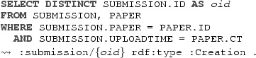
-
The following mapping assertion retrieves from the PAPER table instances of the concept Paper, and instantiates also their features title and type with values of type String.
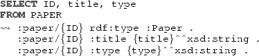
-
The following mapping assertion retrieves from the SUBMISSION table instances of the concept Submission, together with their upload time.
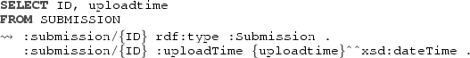
-
Finally, the following mapping assertion retrieves instances of the first component of the reified association Submission, which are pairs of URIs consisting of an instance of the concept Submission, representing the association class, and of an instance of the concept Paper.
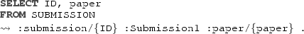


We omit the specification of the mapping assertions for the remaining elements of the conceptual data schema. 
3.5 Processing of Conceptual Queries
When \(\mathcal {{M}}\) is fully defined, it can be used for two purposes. On the one hand, it explicitly documents how the structure of the company information system has to be conceptually understood in terms of domain concepts and relations specified in the conceptual data schema \(\mathcal {{T}}\), and thus constitutes an asset for the company that itself might be worth an investment [31]. On the other hand, \(\mathcal {{S}}=\langle \mathcal {{R}},\mathcal {{T}},\mathcal {{M}}\rangle \) constitutes what we call an OBDA schema, which completely decouples end users from the details of the information system (cf. Fig. 15). Adding to the OBDA schema a database \(\mathcal {{D}}\) that conforms to the database schema \(\mathcal {{R}}\), i.e., replacing \(\mathcal {{R}}\) with an information system \(\mathcal {{I}}\), we obtain what we call an OBDA model \(\mathcal {{B}}=\langle \mathcal {{I}},\mathcal {{T}},\mathcal {{M}}\rangle \). Whenever a user poses a conceptual query q (e.g., expressed in sparql) over \(\mathcal {{T}}\), an OBDA system exploits the OBDA model to answer such query in terms of the data stored in the underlying database \(\mathcal {{D}}\). We sketch now the technique for answering queries in such an OBDA setting [6, 7].
We start with the following observation. Suppose we evaluate (over \(\mathcal {{D}}\)) the queries in the source part of the mapping assertions of \(\mathcal {{M}}\), and we materialize accordingly the corresponding facts in the target part. This would lead to a set of ground facts, denoted by \(\mathcal {{A}}_{\mathcal {{M}},\mathcal {{D}}}\), that can be considered as a \(\textit{DL-Lite}_{\mathcal {{A}}}\) ABox. It can be shown that query answering over \(\mathcal {{B}}\) can be reduced to computing the certain answers over the \(\textit{DL-Lite}_{\mathcal {{A}}}\) ontology \(\mathcal {{O}}=\langle \mathcal {{T}},\mathcal {{A}}_{\mathcal {{M}},\mathcal {{D}}}\rangle \) constituted by the TBox \(\mathcal {{T}}\) and the ABox \(\mathcal {{A}}_{\mathcal {{M}},\mathcal {{D}}}\). However, the query answering algorithm resulting from this approach would need to perform a materialization of \(\mathcal {{A}}_{\mathcal {{M}},\mathcal {{D}}}\), which in general is polynomial in the size of the potentially very large database \(\mathcal {{D}}\), and this might not be practically feasible. However, we can avoid any materialization of the ABox, and rather answer a query q over \(\mathcal {{T}}\) by reformulating it into a new query that can then be evaluated directly over the database \(\mathcal {{D}}\). The resulting query answering algorithm is in general much more efficient than the one based on materialization, and is conceptually divided into three phases, namely rewriting, unfolding, and evaluation, which we briefly describe below.
Rewriting. Given a UCQ q formulated over the conceptual data schema \(\mathcal {{T}}\) of an OBDA schema \(\mathcal {{S}}=\langle \mathcal {{R}},\mathcal {{T}},\mathcal {{M}}\rangle \), and a database \(\mathcal {{D}}\) for \(\mathcal {{R}}\), the rewriting step computes a new UCQ \(q_1\), still over \(\mathcal {{T}}\), in which the logical assertions of \(\mathcal {{T}}\) are compiled in. In computing the rewriting, only inclusion assertions of the form \(E_1\sqsubseteq E_2\) are taken into account, while disjointness assertions \(E_1\sqsubseteq \lnot E_2\) and functionality assertions \((\mathsf {funct}\; Q)\) are not considered. Intuitively, the query q is rewritten, according to the knowledge specified in \(\mathcal {{T}}\) that is relevant for answering q, into a query \(q_1\) such that \( cert (q,\langle \mathcal {{T}},\mathcal {{A}}\rangle )=q_1^{\mathcal {{A}}}\) for every ABox \(\mathcal {{A}}\) for \(\mathcal {{T}}\), where \(q_1^{\mathcal {{A}}}\) denotes the evaluation of \(q_1\) over \(\mathcal {{A}}\), carried out as if \(\mathcal {{A}}\) was a relational database (i.e., under complete knowledge). Hence, the rewriting allows us to get rid of \(\mathcal {{T}}\).
Different query rewriting algorithms have been proposed in the literature, since the first variants that have been presented in [6, 25], to which we refer for more details. We only notice that the rewriting procedure does not depend on the source database \(\mathcal {{D}}\), runs in polynomial time in the size of \(\mathcal {{T}}\), and returns a query \(q_1\) whose size is at most exponential in the size of q (which is also worst-case optimal [32]).
Unfolding. Given the UCQ \(q_1\) over \(\mathcal {{T}}\) computed by the rewriting step, the unfolding step computes, by exploiting the mapping specification \(\mathcal {{M}}\) and using techniques based on partial evaluation of logic programs, an SQL query \(q_2\) that can be directly evaluated over the db schema \(\mathcal {{R}}\). Such a query might return, in addition to values retrieved from \(\mathcal {{D}}\), also URIs constructed according to the URI templates in \(\mathcal {{M}}\). Specifically, the query \(q_2\) is constructed in such a way that \(q_2^{\mathcal {{D}}}=q_1^{A_{\mathcal {{M}},\mathcal {{D}}}}\). Hence, the unfolding allows us to get rid of \(\mathcal {{M}}\). Moreover, also the unfolding procedure does not depend on \(\mathcal {{D}}\), runs in polynomial time in the size of \(\mathcal {{M}}\), and returns a query whose size is at most exponential in the size of \(q_1\).
Evaluation. The evaluation step consists in simply delegating the evaluation of the SQL query \(q_2\), produced by applying first the rewriting step and then the unfolding step, to the RDBMS underlying the information system of the OBDA model. This evaluation step returns \(q_2^{\mathcal {{D}}}\), which is simply the set of tuples resulting from the evaluation of \(q_2\) over \(\mathcal {{D}}\).
Correctness and Complexity of Query Answering. The procedure for processing queries formulated over the conceptual data schema of an OBDA model described above correctly computes the certain answers to UCQs, and it does so by reducing the problem to one of evaluating an SQL query over a relational database. Indeed, we have that \(q_2^{\mathcal {{D}}}=q_1^{A_{\mathcal {{M}},\mathcal {{D}}}}= cert (q,\langle \mathcal {{T}},\mathcal {{A}}_{\mathcal {{M}},\mathcal {{D}}}\rangle )\), and the latter expression corresponds to the answers of Q over \(\mathcal {{B}}\). This means that the problem of computing certain answers to UCQs over an OBDA model is First-Order (FO) rewritable.
We have (implicitly) assumed that, given the database \(\mathcal {{D}}\), the OBDA model \(\mathcal {{B}}\) is consistent, i.e., that the ontology \(\langle \mathcal {{T}},\mathcal {{A}}_{\mathcal {{M}},\mathcal {{D}}}\rangle \) admits at least one model. Notably, it can be shown that the machinery developed for query answering can also be used for checking consistency of \(\mathcal {{B}}\). Therefore, checking consistency can also be reduced to evaluating appropriate SQL queries over the underlying relational database \(\mathcal {{D}}\) [6, 25].
Although the presented query answering technique is computationally worst-case optimal, the increase in size of the queries produced by the rewriting and unfolding steps poses a significant practical challenge. Therefore, a lot of effort has been spent recently in studying the problem of query answering in OBDA and in devising optimization techniques and alternative query transformation approaches that allow for efficient query processing. Discussing these aspects in detail is beyond the scope of the present work, and we refer to the extensive literature on the topic, e.g., [8, 33,34,35]. We remark, however, that many of the optimized techniques for query answering in OBDA have been implemented, both in freely available and in commercial systems. Notable examples are D2RQ Footnote 29, Mastro Footnote 30, Ultrawrap Footnote 31, Morph-RDB Footnote 32, and ontop Footnote 33.
For the implementation of the prototype tools for the preparation phase of process mining based on OBDA that we are discussing in this paper, we rely on the ontop system, which is a state-of-the-art OBDA system available under the very liberal Apache 2 licence. ontop implements the query rewriting and unfolding algorithms discussed above, together with an extensive set of optimization techniques, which are aimed on the one hand at reducing the size of the SQL queries generated by the system, and on the other hand at producing queries that are efficiently executable by relational database engines. We refer to [8] for an in depth discussion of ontop.
4 OBDA for Log Extraction: The onprom Approach
We are now in the position of illustrating how OBDA can be effectively applied to the data preparation phase of process mining. The resulting framework, called onprom, is based on the seminal results in [9, 36]. We start by recalling the methodological steps that are foreseen by onprom, and move then to the formal model and the corresponding toolchain.
4.1 Methodology
The onprom methodology, sketched in Fig. 12, aims at the semi-automatic extraction of event logs from a legacy information system, reflecting different process-related views on the same data, and consequently supporting analysts in the application of process mining along multiple perspectives.

The onprom methodology and its four phases
The methodology comprises four main phases. The first phase is about understanding the meaning of the data stored in the information system at hand. Concretely, it consists of the definition of an OBDA model (cf. Sect. 3), on the one hand providing a conceptual data schema to semantically describe the domain of interest, and on the other hand linking such a data schema to the underlying information system. While this is in general a labor-intensive, purely human activity, if the information system has a “high-level” structure that is understandable by domain experts, such an activity can be partially automatized through bootstrapping techniques [37]. These techniques mirror the schema of the information system into a corresponding conceptual data schema, at the same time generating (identity) mappings to link the two specifications. The result of bootstrapping can then be manually refined.
Once the first phase is completed, process analysts and the other involved stakeholders do not need anymore to consider the structure of the legacy information system, but directly focus on the conceptual data schema. Remember, in fact, that the OBDA paradigm allows one to formulate queries over the conceptual data schema, getting back answers expressed over such a schema but computed over the underlying legacy data.
The goal of the second phase is then to decide which perspective on the data has to be considered for the analysis, singling out, among all possible alternatives, which entities and relationships define the desired notion of case object, and which other conditions have to be defined so as to properly confine the analysis. Recall that a case object represents the main object that is evolved by an instance of the process of interest. E.g., by considering our ConfSys running example, one may decide to focus on the flow of papers submitted to a given conference, or instead tailor the analysis to the flow of operations performed by persons who registered to the conference management system between 2012 and 2015.
4.2 Event Ontology
Since the final goal of data extraction is the generation of a XES event log, the necessary basis for the application of the onprom methodology is to conceptually clarify which key concepts and relations are part of the XES standard. To this end, a (conceptual) event schema is introduced. We denote such an event schema by \(\mathcal {{E}}\). We will see later how such a schema is used to support the semi-automated extraction of an event log from legacy data.
Figure 13 shows the core elements of the event schema:
-
trace, accounting for the evolution of a case through events;
-
event, capturing an atomic step of execution for a case;
-
(simple) attributes, attaching relevant data to traces and events.
Each attribute comes with a key-value pair, and with the characterization of the type taken by the value.

Core event schema

A more comprehensive event schema, capturing all main abstractions of the XES standard
We show now how such a simple schema can be suitably encoded in \(\textit{DL-Lite}_{\mathcal {{A}}}\). To encode the core event schema of Fig. 13, the three concept names Trace, Event, and Attribute are used. In addition, the role names e-has-a, t-has-a, and t-contains-e are used to capture the binary relations among such concepts. To restrict the usage of those role names, the following domain/range axioms are imposed:

Additionally, the following axiom captures that no dangling event may exist, i.e., that each event is assigned to at least one trace:
The typing axioms of the three DL features of the Attribute concept are:

Recall, in fact, that XES attribute values are always stored as strings, while the type information indicates how such string may be parsed into more specific data types.
Finally, by recalling that, in UML, the default multiplicity for an attribute of a class is 1..1, the linkage between the Attribute concept and its three features is captured by the following axioms:

Figure 14 shows a richer event schema that more comprehensively captures the XES standard, including classifiers, global and composite attributes, as well as extensions. However, in the remainder of the paper we will just employ the concepts, relations, and features of the core event schema, making use of the following recurrent attributes to capture key event data, which are encapsulated by XES into specific extensions:
-
timestamp attribute, keeping track of when the event occurred;
-
activity attribute, indicating to which activity the event refers;
-
transition attribute, denoting the type of the event within the lifecycle of the corresponding activity (e.g., whether the event refers to the start, termination, or cancellation of an instance of that activity);
-
resource attribute, indicating the name of the agent responsible for the event occurrence.

Sketch of the onprom model. The dashed mapping specification is automatically generated
4.3 The onprom Model
We describe now the onprom model, whose key elements and their respective relations are depicted in Fig. 15.
We start from the assumption that the data of interest for the analysis is maintained in a legacy information system \(\mathcal {{I}}=\langle \mathcal {{R}},\mathcal {{D}}\rangle \), with schema \(\mathcal {{R}}\) and set \(\mathcal {{D}}\) of facts about the domain of interest. In the typical case where the information system is a relational database, \(\mathcal {{R}}\) accounts for the schema of the tables and their columns, and \(\mathcal {{D}}\) is a set of data structured according to such tables. On top of \(\mathcal {{I}}\), our methodology is centered on the usage of conceptual models in two respects. First, they are used as documentation artifacts that explicitly capture not only knowledge about the domain of interest, but also how legacy information systems relate to that knowledge. This facilitates understanding and interaction among human stakeholders. Second, conceptual models are used as computational artifacts, that is, to automatize the extraction process as much as possible.
The first phase of the methodology consists in the creation of two conceptual models. The first one is the conceptual data schema \(\mathcal {{T}}\), which accounts for the structural knowledge of the domain of interest, i.e., relevant concepts and relations, consequently providing a high-level view of \(\mathcal {{I}}\) that is closer to domain experts. More specifically, we employ UML class diagrams as a concrete language for conceptual data modeling, and we provide their logic-based, formal encoding in terms of the OWL 2 QL ontology language, as illustrated in Sect. 3.2. In the following, depending on the context, we refer to \(\mathcal {{T}}\) as a UML class diagram or as the corresponding OWL 2 QL ontology.
The second conceptual model, the mapping specification \(\mathcal {{M}}\), is a distinctive feature introduced by our approach, borrowed from the area of OBDA. As illustrated in Sect. 3.4, \(\mathcal {{M}}\), which explicitly links \(\mathcal {{I}}\) to \(\mathcal {{T}}\), consists of a set of logical assertions that map patterns of data over schema \(\mathcal {{R}}\) to high-level facts over \(\mathcal {{T}}\).
Once the OBDA system is in place, onprom allows one to abstract away the information system. In this way, the analyst responsible for the data extraction can directly focus on \(\mathcal {{T}}\), using the concepts and relations contained therein so as to concretely formulate which perspective has to be taken towards process mining. More specifically, this amounts to enrich \(\mathcal {{T}}\) with annotations \( \mathcal {{L}} \), each creating an implicit link between \(\mathcal {{T}}\) and the core portion of the event schema \(\mathcal {{E}}\) captured in Fig. 13. In this light, each annotation expresses one of the following aspects:
-
definition of a case, indicating which class provides the basis to identify case objects, and which conditions have to be satisfied by instances of the selected class so as to classify them as case objects;
-
definition of an event, indicating which class provides the basis to identify occurrences of such an event;
-
definition of an event attribute, indicating which navigational route has to be followed within the diagram so as to fetch the value for such an attribute given an instance of the corresponding event.
We consider each type of annotation next.
Case Annotation specifies which class constitutes the main entry point for the analysis, and which additional conditions have to be considered when identifying cases. Each object instantiating this so-called case class, and satisfying the additional conditions, is a case object. Each case object, in turn, is used to correlate the event of interest, grouping into a single trace all the events that refer to the same case object.
Event Annotations pinpoint which events of interest characterise the evolution of the selected case objects, and to which classes of \(\mathcal {{T}}\) they are attached. Only classes that obey to the following two conditions are eligible to be target for an event annotation, i.e., to be marked as event classes. First, the class has to be navigationally connected to the case class. A navigational connection consists of the concatenation of multiple links (i.e., associations or IS-A generalisations), each time imposing that the target class of the current link becomes the source of the next link. Second, the class has to be navigationally connected to a timestamp attribute, through functional associations only.
The first condition is used to establish a relationship between case objects and their related events. The second condition is used to unambiguously identify the execution times associated to those events. It is important to notice that, for both navigations, the concatenated associations may be optional. In this light, only those objects falling under the scope of the annotation, and corresponding to an actual timestamp and to at least one case object, are considered as events. This is used to account for the fact that cases may be still running (i.e., with events that did not occur yet, but that will occur in the future), and that different cases may very well contain different events.
Attribute Annotations capture how to connect events to corresponding values for their characteristic attributes. Each annotation of this form comes with a key that defines the type of targeted attribute, and the specification of a navigational connection to fetch its corresponding value(s). Each event annotation comes with three mandatory attribute annotations, respectively used to capture the relationship between the event and its corresponding case(s), timestamp, and activity. As pointed out before, the timestamp annotation needs to have a functional navigation. This also applies to the activity annotation, with the only difference that, instead of providing a functional navigation, the activity annotation may also be filled with a constant string that independently fixes the name of activity. Beside such three mandatory attributes, additional optional attribute annotations may be provided, so as to cover the various standard extensions provided XES, including the link to a transition within the activity transactional lifecycle, as well as resource information, in turn constituted by the resource name and/or role.

Annotated data model of our ConfSys running example
Example 11
Consider again our ConfSys case study, and in particular the data model shown in Fig. 9, under the assumption that the focus of process mining is to analyse the flow of papers within ConfSys, from their creation and submission to their final judgement. An informal account of the different annotations reflecting this perspective on the data is given in Fig. 16. In particular, the case annotation clearly depicts that each Paper is a case object. On top of this choice for cases, four types of events are identified:
-
Each instance of DecidedPaper may determine a Decision event occurring for that paper instance at the given decision time (attribute decTime). Notice that, in this case, the case class is directly reached from DecidedPaper through its IS-A relationship.
-
Each instance of Creation may determine a Creation event for the paper that is reached by concatenating the IS-A relationship pointing to Submission, together with the Submission association (class), navigating it towards Paper. The event occurs at the upload time attached to the Submission parent class (attribute uploadTime in Submission).
-
Each instance of Submission may determine a Submission for the paper that is obtained by simply navigating the association class Submission towards Paper. Similar to the previous annotation, also events of this type occur at the upload time (attribute uploadTime) for the submission.
-
Finally, each instance of Review may determine a Review event for the paper that is obtained by navigating backward the leadsTo association, in turn navigating the Assignment association (class) towards Paper. The event comes with the timestamp of submission for that review (attribute subTime).

Example 12
A completely different set of annotations would be devised on top of the ConfSys data model in Fig. 9, when considering a class different than Paper to identify cases. For example, one may focus on the flow of operations performed by users of ConfSys, by declaring Person to be the case class. Alternatively, one may consider the flow of review invitations and submissions, by declaring Assignment to be the case class. All such different choices would in turn result in different relevant events and corresponding event/attribute annotations. 
4.4 Formalising Event-Data Annotations
As we have seen, the different event-data annotations enrich the conceptual data schema \(\mathcal {{T}}\) by indicating which classes, associations, and attributes in \(\mathcal {{T}}\) contribute to the identification of cases, events, and event attributes. Towards the automated processing of such annotations, and the consequent automated extraction of an XES event log reflecting such annotations, the first step is to formally represent the annotations using a machine-processable language. To this end, we rely on conjunctive queries encoded as sparql SELECT queries. Such queries are used to extract objects/values targeted by the annotations, and thus change depending on the type of annotation (cf. Sect. 4.3). We review each annotation type next.
Case Annotations are tackled by sparql SELECT queries with a single answer variable, which matches with the intended case objects, i.e., instances of the case class. Additional filters can be expressed in the WHERE clause to single out the boundaries of the analysis (e.g., only papers submitted to a given conference, or within a given timespan, may be considered when analysing ConfSys).
Example 13
The case annotation captured in Fig. 16 can be formalised using the following query:

which retrieves all instances of the Paper class. 
Event Annotations are also tackled using sparql SELECT queries with a single answer variable, this time matching with actual event identifiers, i.e., objects denoting occurrences of events.
Example 14
Consider the event annotation for creation, as shown in Fig. 16. The actual events for this annotation are retrieved using the following query:

which in fact returns all instances of the Creation class. \(\blacksquare \)
Attribute Annotations are formalised using sparql SELECT queries with two answer variables, establishing a relation between events and their corresponding attribute values. In this light, for timestamp and activity attribute annotations, the second answer variable will be substituted by corresponding values for timestamps/activity names. For case attribute annotations, instead, the second answer variable will be substituted by case objects, thus establishing a relationship between events and the case(s) they belong to.
Example 15
Consider again the annotation for creation events, as shown in Fig. 16. The relationship between creation events and their corresponding timestamps is established by the following query:

which indeed retrieves all instances of Creation, together with the corresponding values taken by the uploadTime attribute. \(\blacksquare \)
In the remainder of the paper, a sparql query q formalising an annotation l is called the annotation query for l. Given a set \( \mathcal {{L}} \) of annotations, we denote by \( \mathcal {{L}} _q\) the set of annotation queries formalising the different annotations in \( \mathcal {{L}} \).
4.5 Automated Processing of Annotations
Once the data-annotation step is concluded, the conceptual data schema \(\mathcal {{T}}\) of the input OBDA system \(\langle \mathcal {{I}}, \mathcal {{T}}, \mathcal {{M}}\rangle \) is enriched with annotations \( \mathcal {{L}} \) that implicitly link such a system to the event schema \(\mathcal {{E}}\) that conceptually accounts for the main concepts and relations of the XES standard (cf. Sect. 4.2). We now show how such event-data annotations can be automatically processed, so as to synthesise a new OBDA system that directly maps the data in \(\mathcal {{I}}\) to the event schema \(\mathcal {{E}}\) (cf. the dashed part of Fig. 15). This OBDA system, in turn, can be exploited to query the data in \(\mathcal {{I}}\) as they were structured as a XES event log, and also to actually materialise such an event log.
Technically, onprom takes as input an onprom model \(\mathcal {{P}}=\langle \mathcal {{I}}, \mathcal {{T}}, \mathcal {{M}}, \mathcal {{L}} \rangle \) and the event schema \(\mathcal {{E}}\), and produces new OBDA system \(\langle \mathcal {{I}},\mathcal {{M}}^{\mathcal {{E}}}_{\mathcal {{P}}},\mathcal {{E}}\rangle \), where the annotations in \( \mathcal {{L}} \) are automatically reformulated as OBDA mappings \(\mathcal {{M}}^{\mathcal {{E}}}_{\mathcal {{P}}}\) that directly link \(\mathcal {{I}}\) to \(\mathcal {{E}}\). Such mappings are synthesised using the three-step approach described next.
In the first step, the sparql queries formalising the annotations in \( \mathcal {{L}} \) are reformulated into corresponding SQL queries posed directly over \(\mathcal {{I}}\). This is done by relying on standard query rewriting and unfolding, where each sparql query \(q \in \mathcal {{L}} _q\) is rewritten considering the contribution of the conceptual data schema \(\mathcal {{T}}\), and then unfolded using the mappings in \(\mathcal {{M}}\). The resulting query \(q_{ sql }\) can then be posed directly over \(\mathcal {{I}}\) so as to retrieve the data associated to the corresponding annotation. In the following, we denote the set of all so-obtained SQL queries as \( \mathcal {{L}} _{ sql }\).
Example 16
Consider the sparql query in Example 13, formalising the event annotation that accounts for the creation of papers. A possible reformulation of the rewriting and unfolding of such a query respectively using the conceptual data schema in Fig. 9, and the mappings from Example 10, is the following SQL query:

This query is generated by the ontop OBDA system, which applies various optimisations so as to obtain a final SQL query that is not only correct, but also possibly compact and fast to process by a standard DBMS. One such optimisations is the application of conjunctive query containment techniques to remove parts of the query that are subsumed by others. \(\blacksquare \)
The second step towards the synthesis of \(\mathcal {{M}}^{\mathcal {{E}}}_{\mathcal {{P}}}\) amounts to the creation of the actual, direct mappings from \(\mathcal {{I}}\) to \(\mathcal {{E}}\). Each mapping, in turn, is obtained by considering one of the reformulated annotation queries in \( \mathcal {{L}} _{ sql }\), and constructed depending on the corresponding annotation type. In the obtained mapping, the SQL query constitutes the source part of the mapping, while the annotation type indicates which concepts/roles/features have to be considered to form its target part.
More specifically, \(\mathcal {{M}}^{\mathcal {{E}}}_{\mathcal {{P}}}\) is obtained from \( \mathcal {{L}} _{ sql }\) as follows:
-
1.
For each SQL query \({\texttt {\small q(c)}} \in \mathcal {{L}} _{ sql }\) obtained from a case annotation, we insert into \(\mathcal {{M}}^{\mathcal {{E}}}_{\mathcal {{P}}}\) the following OBDA mapping:
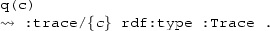
Intuitively, such a mapping populates the concept \(\textit{Trace} \) in \(\mathcal {{E}}\) with the case objects that are created from the answers returned by query \({\texttt {\small q(c)}}\).
-
2.
For each SQL query \({\texttt {\small q(e)}} \in \mathcal {{L}} _{ sql }\) that is obtained from an event annotation, we insert into \(\mathcal {{M}}^{\mathcal {{E}}}_{\mathcal {{P}}}\) the following OBDA mapping:
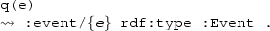
Intuitively, such a mapping populates the concept \(\textit{Event} \) in \(\mathcal {{E}}\) with the event objects that are created from the answers returned by query \({\texttt {\small q(e)}}\).
-
3.
For each SQL query \({\texttt {\small q(e,y)}} \in \mathcal {{L}} _{ sql }\) that is obtained from an attribute annotation, we insert into \(\mathcal {{M}}^{\mathcal {{E}}}_{\mathcal {{P}}}\) a mapping that depends on the type of attribute:
-
(a)
If \({\texttt {\small q(e,y)}}\) is the query obtained from a case attribute annotation (i.e., \({\texttt {\small e}}\) is bound to events, and \({\texttt {\small y}}\) to their corresponding cases), then the mapping has the following form:

Intuitively, such a mapping populates the the relation that links traces and events in \(\mathcal {{E}}\) (i.e., the role t-contains-e) with the answers returned by query \({\texttt {\small q(e,y)}}\).
-
(b)
If \({\texttt {\small q(e,y)}}\) is the query obtained from a timestamp attribute annotation (i.e., \({\texttt {\small e}}\) is bound to events, and \({\texttt {\small y}}\) to their corresponding execution times), then the mapping has the following form:
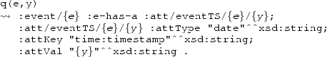
Intuitively, such a mapping populates the concept Attribute with the objects representing timestamp attributes. at the same time, it also suitably reconstruct the event-timestamp relationship at the level of \(\mathcal {{E}}\), using the answers returned by query \({\texttt {\small q(e,y)}}\).
-
(c)
If \({\texttt {\small q(e,n)}}\) is the query obtained from an activity attribute annotation (i.e., \({\texttt {\small e}}\) is bound to events, and \({\texttt {\small n}}\) to their corresponding activity names), then the mapping has the following form:
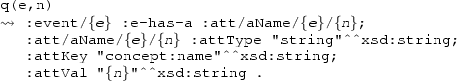
-
(a)


It is worth noting that the presented approach can be straightforwardly generalised to cover additional types of annotations (e.g., dealing with the activity transactional lifecycle, or the involved resources).
The third, final step consists in leveraging the synthesised OBDA system \(\langle \mathcal {{I}}, \mathcal {{E}}, \mathcal {{M}}^{\mathcal {{E}}}_{\mathcal {{P}}}\rangle \) so as to extract the event data of interest. The extraction can be declaratively guided by formulating sparql queries over the vocabulary of \(\mathcal {{E}}\) and, if needed, serialising the obtained answers in the form of an XES event log. We provide, in the following, a list of sparql queries serving this purpose.
The sparql query below retrieves events and their attributes, considering only those events that do actually have a reference trace, timestamp, and activity name:

The WHERE clause is used to filter away dangling events (i.e., events for which the corresponding case is not known), or events with missing timestamp or missing activity name.
The following query is instead meant to retrieve (elementary) attributes, considering in particular their key, type, and value.

The following query handles the retrieval of empty and nonempty traces, simultaneously obtaining, for nonempty traces, their constitutive events:

4.6 The onprom Toolchain
onprom comes with a toolchain that supports the various phases of the methodology shown in Fig. 12, and in particular implements the automated processing technique for annotations discussed in Sect. 4.5. The toolchain is open source and can be downloaded from http://onprom.inf.unibz.it. The toolchain is available as a stand-alone software, or as a set of plugins running inside the ProM process mining framework. Specifically, the onprom toolchain consists of the following components:
-
a UML Editor to model the conceptual data schema (cf. Sect. 4.1);
-
an Annotation Editor to enrich the conceptual data schema with event-data annotations (cf. Sect. 4.3);
-
a Log Extractor component that automatically processes the event-data annotations, and extracts an XES event log from a given relational information system (cf. Sect. 4.5).
Notice that the definition of a suitable mapping specification to link a conceptual data schema to an underlying information system is not natively covered within onprom, and we assume that it is realised manually or by exploiting third-party tools, such as the ontop mapping editor for ProtégéFootnote 34.
We now briefly describe each component, using ConfSys as running example.

The onprom UML Editor, showing the conceptual data schema used in our ConfSys running example
UML Editor. The UML editor provides two main functionalities: modelling of a UML class diagram, and import/export from/to OWL 2 QL, leveraging the correspondence described in Sect. 3.2. The editor makes some simplifying assumptions, in line with this correspondence with OWL 2 QL:
-
we do not support completeness of UML generalisation hierarchies, since the presence of such construct would fundamentally undermine the virtual OBDA approach based on query reformulation [7];
-
in line with Semantic Web languages, we explicitly support binary associations only;
-
multiplicities in associations (resp., features) are restricted to be either 0 or 1. Hence, we can express functionality and mandatory participation;
-
we do not support IS-A between associations;
-
we ignore all those features that are not directly related to conceptual modelling, but instrumental to software design, such as stereotypes and methods.
A screenshot of the UML Editor showing the conceptual data schema of ConfSys is shown in Fig. 17.
Annotation Editor. This editor supports data and process analysts in the specification of event-data annotations on top of a UML class diagram developed using the UML editor described above.

The Annotation Editor showing annotations for the ConfSys use case

The properties of event annotations defined for the ConfSys use case
A screenshot of the Annotation Editor, showing annotations for our ConfSys conceptual data schema, is shown Fig. 18. Specifically, the screenshot shows that Paper has been annotated as case class, and that four events annotations are defined, implementing what is reported in Fig. 16 (together with additional attribute definitions). The input forms for the configurations of such annotations are depicted in Fig. 19.
To simplify the annotation task, the editor supports some advanced operations:
-
Properties and paths can be chosen using navigational selections over the diagram via mouse-click operations.
-
The editor takes into account multiplicities on associations and attributes; when the user is selecting properties of the case and of events (in particular the timestamp), the editor enables only navigation paths that are functional.
The annotations are automatically translated into corresponding sparql queries by the editor.
Log Extraction Plug-in. The last component of the toolchain implements the mapping synthesis technique described in Sect. 4.5 towards log extraction, leveraging the state-of-the-art ontop framework to handle several important tasks such as (i) management of OBDA mappings, (ii) rewriting and unfolding of sparql queries, and (iii) query answering. In addition, the log extraction component exploits the OpenXES APIsFootnote 35 for managing XES data structures and the corresponding XML serialisation. Figure 20 shows the screenshot of the log extractor plug-in in Prom 6.6. Essentially, the plug-in takes the following inputs:
-
1.
A conceptual data schema \(\mathcal {{T}}\), generated via the UML Editor or represented as an OWL 2 QL file;
-
2.
An OBDA mapping specification, containing
-
a mapping specification \(\mathcal {{M}}\) linking \(\mathcal {{T}}\) to an underlying relational \(\mathcal {{R}}\)
-
the connection information to access a database instance \(\mathcal {{D}}\) of interest, conforming to \(\mathcal {{R}}\).
-
-
3.
Event-data annotations \( \mathcal {{L}} \), which can be created using the Annotation Editor.

Screenshot of Log Extractor Plug-in in Prom 6.6.
As output, the plugin produces a XES event log obtained as the result of the processing of the database instance \(\mathcal {{D}}\) through the provided mappings and annotations. The event log is offered as a standard ProM resource within the ProM framework.
5 Conclusions
In this paper, we have presented the onprom framework, which leverages techniques from intelligent data management to tackle the challenging phase of data preparation for process mining, enabling the possibility to apply process mining techniques on top of legacy information systems. Instead of forcing data and process analysts to set up ad-hoc, manual extraction procedures, onprom provides support to handle this problem at a higher level of abstraction. Specifically, users focus on modelling the data of interest conceptually, on the one hand linking the resulting conceptual schema to legacy data via declarative mappings, and on the other hand equipping the schema with declarative annotations that indicate where cases, events, and their attributes are “located” within such a schema. onprom then automatises the extraction of event logs, manipulating and reasoning over mappings and annotations by exploiting well-established techniques from knowledge representation and ontology-based data access.
We believe that the synergic integration of techniques coming from data and process management is the key to enable decision makers, analysts and domain experts in improving the way work is conducted within small, medium and large enterprises. At the same time, it provides interesting, open research challenges for computer scientists, covering both foundational and applied aspects. In particular, different interesting lines of research can be developed starting from onprom, ranging from the optimisation of ontology-based data access in the specific context of event log extraction, to the investigation of techniques and methodologies for event modelling and recognition typically studied within formal ontology, to the definition of alternative mechanisms for linking conceptual data schemas to reference, event log models.
Notes
- 1.
Small and medium-sized enterprises.
- 2.
- 3.
Enterprise Resource Planning.
- 4.
Customer Relationship Management.
- 5.
Supply Chain Management.
- 6.
- 7.
- 8.
- 9.
- 10.
- 11.
- 12.
- 13.
- 14.
- 15.
- 16.
- 17.
- 18.
- 19.
- 20.
- 21.
- 22.
- 23.
We consider here the case of an information system consisting of a single relational data source. Multiple data sources can be wrapped by a federation tool and presented as a single source.
- 24.
In \(\textit{DL-Lite}_{\mathcal {{A}}}\), features are actually called attributes. Here we use the term “feature” to avoid confusion with attributes of UML (see later).
- 25.
See http://www.omg.org/spec/UML/2.5/ for the latest version of UML at the moment of writing.
- 26.
If the roles of the association are not specified in the UML class diagram, we may use arbitrary fresh DL role names, each of which is identified by the name of the association and the component.
- 27.
- 28.
The formal counterpart of such an SQL query is a first-order logic (FOL) query with distinguished variables \(\vec {x}\).
- 29.
- 30.
- 31.
- 32.
- 33.
- 34.
- 35.
References
Dumas, M., Rosa, M.L., Mendling, J., Reijers, H.A.: Fundamentals of Business Process Management. Springer, Heidelberg (2013)
Weske, M.: Business Process Management - Concepts, Languages, Architectures, 2nd edn. Springer, Heidelberg (2012)
van der Aalst, W., et al.: Process mining manifesto. In: Daniel, F., Barkaoui, K., Dustdar, S. (eds.) BPM 2011. LNBIP, vol. 99, pp. 169–194. Springer, Heidelberg (2012). doi:10.1007/978-3-642-28108-2_19
van der Aalst, W.M.P.: Process Mining - Data Science in Action, 2nd edn. Springer, Heidelberg (2016)
IEEE Computational Intelligence Society: IEEE Standard for eXtensible Event Stream (XES) for Achieving Interoperability in Event Logs and Event Streams. IEEE Std 1849–2016 (2016). i–50
Poggi, A., Lembo, D., Calvanese, D., Giacomo, G., Lenzerini, M., Rosati, R.: Linking data to ontologies. In: Spaccapietra, S. (ed.) Journal on Data Semantics X. LNCS, vol. 4900, pp. 133–173. Springer, Heidelberg (2008). doi:10.1007/978-3-540-77688-8_5
Calvanese, D., Giacomo, G., Lembo, D., Lenzerini, M., Poggi, A., Rodriguez-Muro, M., Rosati, R.: Ontologies and databases: the DL-Lite approach. In: Tessaris, S., Franconi, E., Eiter, T., Gutierrez, C., Handschuh, S., Rousset, M.-C., Schmidt, R.A. (eds.) Reasoning Web 2009. LNCS, vol. 5689, pp. 255–356. Springer, Heidelberg (2009). doi:10.1007/978-3-642-03754-2_7
Calvanese, D., Cogrel, B., Komla-Ebri, S., Kontchakov, R., Lanti, D., Rezk, M., Rodriguez-Muro, M., Xiao, G.: Ontop: answering SPARQL queries over relational databases. Semant. Web J. 8(3), 471–487 (2017)
Calvanese, D., Kalayci, T.E., Montali, M., Tinella, S.: Ontology-based data access for extracting event logs from legacy data: the onprom tool and methodology. In: Abramowicz, W. (ed.) BIS 2017. LNBIP, vol. 288, pp. 220–236. Springer, Heidelberg (2017). https://www.springer.com/us/book/9783319593357
van der Aalst, W., Weijters, T., Maruster, L.: Workflow mining: discovering process models from event logs. IEEE Trans. Knowl. Data Eng. 16(9), 1128–1142 (2004)
Leemans, S.J.J., Fahland, D., van der Aalst, W.M.P.: Process and deviation exploration with inductive visual miner. In: Proceedings of BPM Demo Sessions. CEUR Workshop Proceedings, vol. 1295, p. 46. CEUR-WS.org (2014). http://ceur-ws.org/
Eck, M.L., Lu, X., Leemans, S.J.J., van der Aalst, W.M.P.: PM\(^2\): a process mining project methodology. In: Zdravkovic, J., Kirikova, M., Johannesson, P. (eds.) CAiSE 2015. LNCS, vol. 9097, pp. 297–313. Springer, Cham (2015). doi:10.1007/978-3-319-19069-3_19
Verbeek, H.M.W., Buijs, J.C.A.M., Dongen, B.F., van der Aalst, W.M.P.: XES, XESame, and ProM 6. In: Soffer, P., Proper, E. (eds.) CAiSE Forum 2010. LNBIP, vol. 72, pp. 60–75. Springer, Heidelberg (2011). doi:10.1007/978-3-642-17722-4_5
Dongen, B.F., Medeiros, A.K.A., Verbeek, H.M.W., Weijters, A.J.M.M., van der Aalst, W.M.P.: The ProM framework: a new era in process mining tool support. In: Ciardo, G., Darondeau, P. (eds.) ICATPN 2005. LNCS, vol. 3536, pp. 444–454. Springer, Heidelberg (2005). doi:10.1007/11494744_25
van der Aalst, W.M.P., Bolt, A., van Zelst, S.J.: RapidProM: Mine your processes and not just your data. CoRR Technical Report abs/1703.03740, arXiv.org e-Print archive, March 2017. http://arxiv.org/abs/1703.03740
Günther, C.W., Rozinat, A.: Disco: discover your processes. In; Lohmann, N., Moser, S. (eds.) Proceedings of the Demonstration Track of the 10th International Conference on Business Process Management (BPM). CEUR Workshop Proceedings, vol. 940, pp. 40–44 (2012). http://ceur-ws.org/
Günther, C.W.: XES Standard Definition Version 1.0. Technical report, Fluxicon Process Laboratories, November 2009. http://www.xes-standard.org
van Dongen, B.F., van der Aalst, W.M.P.: A meta model for process mining data. In: Proceedings of EMOI - INTEROP. CEUR Workshop Proceedings, vol. 160. CEUR-WS.org (2005). http://ceur-ws.org/
Günther, C.W., Verbeek, E.: XES Standard Definition Version 2.0. Technical report, Fluxicon Process Laboratories, March 2014. http://www.xes-standard.org
Günther, C.W., Aalst, W.M.P.: A generic import framework for process event logs. In: Eder, J., Dustdar, S. (eds.) BPM 2006. LNCS, vol. 4103, pp. 81–92. Springer, Heidelberg (2006). doi:10.1007/11837862_10
Bao, J., et al.: OWL 2 Web Ontology Language document overview, 2nd edn. W3C Recommendation, World Wide Web Consortium, December 2012. http://www.w3.org/TR/owl2-overview/
Baader, F., Calvanese, D., McGuinness, D., Nardi, D., Patel-Schneider, P.F. (eds.): The Description Logic Handbook: Theory, Implementation and Applications. Cambridge University Press (2003)
Calvanese, D.: Query answering over description logic ontologies. In: Fermé, E., Leite, J. (eds.) JELIA 2014. LNCS (LNAI), vol. 8761, pp. 1–17. Springer, Cham (2014). doi:10.1007/978-3-319-11558-0_1
Vardi, M.Y.: The complexity of relational query languages. In: Proceedings of the 14th ACM SIGACT Symposium on Theory of Computing (STOC), pp. 137–146 (1982)
Calvanese, D., De Giacomo, G., Lembo, D., Lenzerini, M., Rosati, R.: Tractable reasoning and efficient query answering in description logics: The DL-Lite family. J. Autom. Reasoning 39(3), 385–429 (2007)
Calvanese, D., De Giacomo, G., Lembo, D., Lenzerini, M., Rosati, R.: Data complexity of query answering in description logics. Artif. Intell. 195, 335–360 (2013)
Motik, B., Cuenca Grau, B., Horrocks, I., Wu, Z., Fokoue, A., Lutz, C.: OWL 2 Web Ontology Language profiles, 2nd edn. W3C Recommendation, World Wide Web Consortium, December 2012. http://www.w3.org/TR/owl2-profiles/
Calvanese, D., Lenzerini, M., Nardi, D.: Unifying class-based representation formalisms. J. Artif. Intell. Res. 11, 199–240 (1999)
Berardi, D., Calvanese, D., De Giacomo, G.: Reasoning on UML class diagrams. Artif. Intell. 168(1–2), 70–118 (2005)
Abiteboul, S., Hull, R., Vianu, V.: Foundations of Databases. Addison Wesley Publ. Co. (1995)
Antonioli, N., Castanò, F., Coletta, S., Grossi, S., Lembo, D., Lenzerini, M., Poggi, A., Virardi, E., Castracane, P.: Ontology-based data management for the Italian public debt. In: Proceedings of the 8th International Conference on Formal Ontology in Information Systems (FOIS). Frontiers in Artificial Intelligence and Applications, vol. 267, pp. 372–385. IOS Press (2014)
Gottlob, G., Kikot, S., Kontchakov, R., Podolskii, V.V., Schwentick, T., Zakharyaschev, M.: The price of query rewriting in ontology-based data access. Artif. Intell. 213, 42–59 (2014)
Kontchakov, R., Lutz, C., Toman, D., Wolter, F., Zakharyaschev, M.: The combined approach to query answering in DL-Lite. In: Proceedings of the 12th International Conference on the Principles of Knowledge Representation and Reasoning (KR), pp. 247–257 (2010)
Rodriguez-Muro, M., Calvanese, D.: High performance query answering over DL-Lite ontologies. In: Proceedings of the 13th International Conference on the Principles of Knowledge Representation and Reasoning (KR), pp. 308–318 (2012)
Rodriguez-Muro, M., Rezk, M.: Efficient SPARQL-to-SQL with R2RML mappings. J. Web Semant. 33, 141–169 (2015)
Syamsiyah, A., van Dongen, B.F., van der Aalst, W.M.P.: DB-XES: enabling process discovery in the large. In: Ceravolo, P., Guetl, C., Rinderle-Ma, S. (eds.) Proceedings of the 6th International Symposium on Data-driven Process Discovery and Analysis (SIMPDA). CEUR Workshop Proceedings, vol. 1757, pp. 63–77 (2016). http://ceur-ws.org/
Jiménez-Ruiz, E., Kharlamov, E., Zheleznyakov, D., Horrocks, I., Pinkel, C., Skjæveland, M.G., Thorstensen, E., Mora, J.: BootOX: Bootstrapping OWL 2 Ontologies and R2RML Mappings from Relational Databases. In Villata, S., Pan, J.Z., Dragoni, M. (eds.) Proceedings of the 14th International Semantic Web Conference Posters & Demonstrations Track (ISWC). CEUR Workshop Proceedings, vol. 1486 (2015). http://ceur-ws.org/
Acknowledgements
This research has been partially supported by the Euregio IPN12 “KAOS: Knowledge-Aware Operational Support” project, which is funded by the “European Region Tyrol-South Tyrol-Trentino” (EGTC) under the first call for basic research projects, and by the UNIBZ internal project “OnProm (ONtology-driven PROcess Mining)”. We thank Wil van der Aalst for the interesting discussions and insights on the problem of extracting event logs from legacy information systems.
Author information
Authors and Affiliations
Corresponding author
Editor information
Editors and Affiliations
Rights and permissions
Copyright information
© 2017 Springer International Publishing AG
About this chapter
Cite this chapter
Calvanese, D., Kalayci, T.E., Montali, M., Santoso, A. (2017). OBDA for Log Extraction in Process Mining. In: Ianni, G., et al. Reasoning Web. Semantic Interoperability on the Web. Reasoning Web 2017. Lecture Notes in Computer Science(), vol 10370. Springer, Cham. https://doi.org/10.1007/978-3-319-61033-7_9
Download citation
DOI: https://doi.org/10.1007/978-3-319-61033-7_9
Published:
Publisher Name: Springer, Cham
Print ISBN: 978-3-319-61032-0
Online ISBN: 978-3-319-61033-7
eBook Packages: Computer ScienceComputer Science (R0)