POSL: A Parallel-Oriented Metaheuristic-Based Solver Language

Abstract

For a couple of years, all processors in modern machines are multi-core. Massively parallel architectures , so far reserved for super-computers, become now available to a broad public through hardware like the Xeon Phi or GPU cards. This architecture strategy has been commonly adopted by processor manufacturers, allowing them to stick with Moore’s law. However, this new architecture implies new ways to design and implement algorithms to exploit its full potential. This is in particular true for constraint-based solvers dealing with combinatorial optimization problems. Here we propose a Parallel-Oriented Solver Language (POSL, pronounced “puzzle”), a new framework to build interconnected meta-heuristic based solvers working in parallel. The novelty of this approach lies in looking at solver as a set of components with specific goals, written in a parallel-oriented language based on operators. A major feature in POSL is the possibility to share not only information, but also behaviors, allowing solver modifications during runtime. Our framework has been designed to easily build constraint-based solvers and reduce the developing effort in the context of parallel architecture. POSL’s main advantage is to allow solver designers to quickly test different heuristics and parallel communication strategies to solve combinatorial optimization problems, usually time-consuming and very complex technically, requiring a lot of engineering.

6.1 Introduction

Combinatorial Optimization has strong applications in several fields, including machine learning, artificial intelligence, and software engineering. In some cases, the main goal is only to find a solution, like for Constraint Satisfaction Problems (CSP). A solution will be an assignment of variables satisfying the constraints set. In other words: finding one feasible solution.

CSPs find a lot of applications in the industry, implying the development of many methods to solve them. Meta-heuristics techniques have shown themselves to be effective for solving CSPs, but in most industrial cases the search space is huge enough to be intractable. However, recent advances in computer architecture are leading us toward massively multi/many-core computers, opening a new way to find solutions for these problems in a more feasible manner, reducing search time. Adaptive Search [5] is an efficient methods showing very good performances scaling to hundreds or even thousands of cores, using a multi-walk local search method. For this algorithm, an implementation of a cooperative multi-walks strategy has been published in [9]. These works have shown the efficiency of multi-walk strategy, that is why we have oriented POSL towards this parallel scheme.

In the last years, a lot of efforts have been made in parallel constraint programming. In this field, the inter-process communication for solver cooperation is one of the most critical issues. Pajot and Monfroy [11] presents a paradigm that enables the user to properly separate strategies combining solver applications in order to find the desired result, from the way the search space is explored. Meta-S is an implementation of a theoretical framework proposed in [6], which allows to tackle problems, through the cooperation of arbitrary domain-specific constraint solvers. POSL provides a mechanism of creating solver-independent communication strategies, making easy the study of solving processes and results. Creating solvers implementing different solution strategies can be complex and tedious. In that sense POSL gives the possibility of prototyping communicating solvers with few efforts.

In Constraint Programming, many researches focus on fitting and improving existing algorithms for specific problems. However, it requires a deep study to find the right algorithm for the right problem. Hyperion [3] is a Java framework for meta- and hyper-heuristics built with the principle of interoperability, generality by providing generic templates for a variety of local search and evolutionary computation algorithms and efficiency, allowing rapid prototyping with the possibility of reusing source code. POSL aims to offer the same advantages, but provides also a mechanism to define communication protocols between solvers.

In this chapter we present POSL, a framework for easily building many and different cooperating solvers based on coupling four fundamental and independent components: operation modules, open channels, the computation strategy and communication channels or subscriptions. Recently, the hybridization approach leads to very good results in constraint satisfaction [14]. ParadisEO is a framework to design parallel and distributed hybrid meta-heuristics showing very good results [4]. It includes a broad range of reusable features to easily design evolutionary algorithms and local search methods. Our framework POSL focuses only in local search methods, but is designed to execute in parallel sets of different solvers, with and/or without communication, since the solver’s components can be combined by using operators.

POSL provides, through a simple operator-based language, a way to create a computation strategy, combining already defined components (operation modules and open channels). A similar idea was proposed in [7] without communication, introducing an evolutionary approach that uses a simple composition operator to automatically discover new local search heuristics for SAT and to visualize them as combinations of a set of building blocks. Another interesting idea is proposed in Templar, a framework to generate algorithms changing predefined components using hyper-heuristics methods [13]. In the last phase of the coding process with POSL, solvers can be connected each others, depending on the structure of their open channels, and this way, they can share not only information, but also their behavior, by sharing their operation modules. This approach makes the solvers able to evolve during the execution.

Before ending this chapter with a brief conclusion and future works, we present some results obtained by using POSL to solve some instances of the Social Golfers Problem.

6.2 POSL Parallel Solvers

POSL proposes a solver construction platform following different stages. First of all, the solver algorithm is modeled by decomposing it into small pieces/modules of computation. After that, they are implemented as separated functions. We name them operation module. The next step is to decide what information is interesting to receive from other solvers. This information is encapsulated into other objects called open channels, allowing data transmission among solvers. In a third stage, a generic strategy is coded through POSL, using the mentioned components in the previous stages, allowing not only the information exchange, but also to execute the components in parallel. This will be the solver’s backbone. Finally, solvers are defined by instantiating and connecting the strategy, operation modules and open channels, and by connecting them each others. The next subsections explain in details each of these steps.

6.2.1 Operation Module

An operation module is the most basic and abstract way to define a piece of computation. It can be dynamically replaced by or combined with other operation modules, since they can be sheared among solvers working in parallel. This way, the solver can mutate its behavior during execution.

An operation module receives an input, executes an internal algorithm and gives an output. They are joined through computation strategies.

Definition 6.1.

Operation Module An operation module Om is a mapping defined by:

$$\displaystyle{ Om: D \rightarrow I }$$

(6.1)

D and I can be either a set of configurations, or set of sets of configurations, or a set of values of some data type, etc.

Consider a local search meta-heuristic solver. One of its operation modules can be the function returning the set of configurations composing the neighborhood of a given configuration:

$$\displaystyle{ Om_{neighborhood}: D_{1} \times D_{2} \times \ldots \times D_{n} \rightarrow 2^{D_{1}\times D_{2}\times \ldots \times D_{n} } }$$

where D _i represents the definition domains of each variable of the input configuration.

6.2.2 Open Channels

Open Channels are the solver’s components in charge of the information reception in the communication between solvers. They can interact with operation modules, depending on the computation strategy. Open Channels play the role of outlets, allowing solvers to be connected and to share information.

An open channel can receive two types of information, always coming from an external solver: data or operation modules. It is important to notice that when we are talking about sending/receiving operation modules, we mean sending/receiving only required information to identify it and being able to instantiate it.

In order to distinguish between the two different types of open channels, we will call Data Open Channel the open channel responsible for the data reception, and Object Open Channel the one responsible for the reception and instantiation of operation modules.

Definition 6.2.

Data Open Channel A Data Open Channel Ch is a component that produces a mapping defined as follows:

$$\displaystyle{ Ch: U \rightarrow I }$$

(6.2)

It returns the information I coming from an external solver, no matter what the input U is.

Definition 6.3.

Object Open Channel If we denote by $\mathbb{M}$ the space of all the operation modules defined by Definition 6.1, then an Object Open Channel Ch is a component that produces an operation module coming from an external solver as follows:

$$\displaystyle{ Ch: \mathbb{M} \rightarrow \mathbb{M} }$$

(6.3)

Due to the fact that open channels receive information coming from outside and have no control on them, it is necessary to define the NULL information, to denote the absence of any information. If a Data Open Channel receives a piece of information, it is returned automatically. If a Object Open Channel receives an operation module, the latter is instantiated and executed with the open channel’s input, and its result is returned. In both cases, if no available information exists (no communications are performed), the open channel returns the NULL object.

6.2.3 Computation Strategy

The computation strategy is the solver’s backbone: it joins operation modules and open channels in a coherent way, while remaining independent from them. Through the computation strategy we can decide also what information to sent to other solvers.

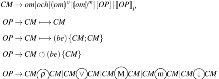
The computation strategy is an operator-based language, that we define as a free-context grammar as follows:

Definition 6.4.

POSL’s Grammar $G_{POSL} = \left (\mathbf{V},\varSigma,\mathbf{S},\mathbf{R}\right )$, where:

• 1. $\mathbf{V} = \left \{CM,OP\right \}$ is the set of variables,

• 2. is the set of terminals,

• 3. $\mathbf{S} = \left \{CM\right \}$ is the set of start variables,

• 4. and the set of rules R =

  

We would like to explain some of the concepts presented in Definition 6.4:

• The variable CM, as well as OP are two entities very important in the language, as can be seen in the grammar. We name them compound module and operator respectively.

• The terminals om and och represent an operation module and an open channel respectively,

• The terminal be is a boolean expression.

• The terminals [ ],  _p are symbols for grouping and defining the way of how the involved compound modules are executed. Depending on the nature of the operator, they can be executed sequentially or in parallel:

  • 1. $\left [\text{OP}\right ]$: The involved operator is executed sequentially.

  • 2. OP _p : The involved operator is executed in parallel if and only if OP supports parallelism. Otherwise, an exception is threw.

• The terminals ( and ) are symbols for grouping the boolean expression in some operators.

• The terminals { and } are symbols for grouping compound modules in some operators.

• The terminals are operators to send information to other solvers (explained bellow).

• The rest of terminals are POSL operators.

6.2.3.1 POSL Operators

In this section we briefly present operators provided by POSL to code the computation strategy. A formal presentation of POSL’s specification is available in [12].

• $\fbox{ $Op.\,\,1: $}$ Operator Sequential Execution: the operation M ₁ ↦ M ₂ represents a compound module as result of the execution of M ₁ followed by M ₂. This operator is an example of an operator that does not support the execution of its involved compound modules in parallel, because the input of the second compound module is the output of the first one.

• $\fbox{ $Op.\,\,2: $}$ Operator Conditional Sequential Execution: the operation

  $M_{1}\longmapsto (<cond>)\left \{M_{2},M_{3}\right \}$ represents a compound module as result of the sequential execution of M ₁ followed by M ₂ if < cond > is true or by M ₃ otherwise.

• $\fbox{ $Op.\,\,3: $}$ Operator Cyclic Execution: the operation $\circlearrowleft (<cond>)\left \{I_{1}\right \}$ represents a compound module as result of the sequential execution of I ₁ repeated while < cond > remains true.

• $\fbox{ $Op.\,\,4: $}$ Operator Random Choice: the operation represents a compound module that executes and returns the output of M ₁ depending on the probability ρ, or M ₂ following (1 −ρ)

• $\fbox{ $Op.\,\,5: $}$ Operator Not NULL Execution: the operation represents a compound module that executes M ₁ if it is not NULL or M ₂ otherwise.

• $\fbox{ $Op.\,\,6: $}$ Operator MAX: the operation represents a compound module that returns the maximum between the outputs of modules M ₁ and M ₂ (tacking into account some order criteria).

• $\fbox{ $Op.\,\,7: $}$ Operator MIN: the operation represents a compound module that returns the minimum between the outputs of modules M ₁ and M ₂ (tacking into account some order criteria).

• $\fbox{ $Op.\,\,8: $}$ Operator Speed: the operation represents a compound module that returns the output of the module ending first.

In Fig. 6.1 we present a simple example of how to combine modules using POSL operators introduced above. Algorithm 1 shows the corresponding code. In this example we show four operation modules being part of a compound module representing a dummy local search method. In this example:

Fig. 6.1

Un example of a basic solver using POSL

• M ₁: generates a random configuration.

• M ₂: computes a neighborhood of a given configuration by selecting a random variable and changing its value.

• M ₃: computes a neighborhood of a given configuration by selecting K random variables and changing theirs values.

• M ₄: selects, from a set of configurations, the one with the smallest cost, and stores it.

Here, the operation module M ₂ is executed with probability ρ, and M ₃ is executed with probability (1 −ρ). This operation is repeated a number N of times (< stop_cond >).

Algorithm 1 POSL code for Fig. 6.1

In Algorithm 1, loops represent the number of iterations performed by the operator.

• $\fbox{ $Op. - 8: $}$ Operator Sending: allows us to send two types of information to other solvers:

  • 1. The operation represents a compound module that executes the compound module M and sends its output

  • 2. The operation represents a compound module that executes the compound module M and sends M itself

Algorithm 2 POSL code for Fig. 6.2 case (1)

Algorithm 3 POSL code for Fig. 6.2 case (2)

Algorithms 2 and 3 show POSL’s code corresponding to Fig. 6.2 for both cases: (a) sending the result of the execution of the operation module M, or (b) sending the operation module M itself.

Fig. 6.2

Sending Information Operator

This operation is very useful in terms of sharing behaviors between solvers. Figure 6.3 shows another example, where we can combine an open channel with the operation module M ₂ through the operator . In this case, the operation module M ₂ will be executed as long as the open channel remains NULL, i.e. there is no operation module coming from outside. This behavior is represented in Fig. 6.3 by red lines. If some operation module has been received by the open channel, it is executed instead of the operation module M ₂, represented in Fig. 6.3 by blue lines.

Fig. 6.3

Two different behaviors in the same solver. (a) The solver executes his own operation module if no information is received through the open channel. (b) The solver executes the operation module coming from an external solver

In this stage, and using these operators, we can create the algorithm managing different components to find the solution of a given problem. These algorithms are fixed, but generic w.r.t. their components (operation modules and open channels). It means that we can build different solvers using the same strategy, but instantiating it with different components, as long as they have the right input/output signature.

To define a computation strategy we use the environment presented in Algorithm 6, where M _i and Ch _i represent the types of the operation modules and the types of the open channels used by the computation strategy St. Between brackets, the field < ...computation strategy... > corresponds to POSL code based on operators combining already declared modules.

Algorithm 4 Computation strategy definition

      St ← strategy

      oModule M ₁, M ₂, …, M _n

      oChannel Ch ₁, Ch ₂, …, Ch _m

      {

      <...computation strategy... >

      }

Algorithm 5 Solver definition

      solver _k ← solver

      {

      cStrategy St

      oModule m ₁, m ₂, …, m _n

      oChannel ch ₁, ch ₂, …, ch _m

      }

6.2.4 Solver Definition

With operation modules, open channels and computation strategy defined, we can create solvers by instantiating the declared components. POSL provides an environment to this end, presented in Algorithm 6, where m _i and ch _i represent the instances of the operation modules and the instances of the open channels to be passed by parameters to the computation strategy St.

6.2.5 Communication Definition

Once we have defined our solver strategy, the next step is to declare communication channels, i.e. connecting the solvers each others. Up to here, solvers are disconnected, but they have everything to establish the communication. In this last stage, POSL provides to the user a platform to easily define cooperative meta-strategies that solvers must follow.

The communication is established by following the next rules guideline:

• 1. Each time a solver sends any kind of information by using the operator or , it creates a communication jack

• 2. Each time a solver uses an open channel into its definition, it creates a communication outlet

• 3. Solvers can be connected each others by creating subscriptions, connecting communication jacks with communication outlet (see Fig. 6.4).

  Fig. 6.4

  

  Three solvers composing the POSL-solver

With the operator (⋅ ) we have access to operation modules sending information and to the open channel’s names in a solver. For example: Solver ₁ ⋅ M ₁ provides access to the operation module M ₁ in Solver ₁ if and only if it is affected by the operator (or ), and Solver ₂ ⋅ Ch ₂ provides access to the open channel Ch ₂ in Solver ₂. Tacking this into account, we can define the subscriptions.

Definition 6.5.

Let two different solvers Solver ₁ and Solver ₂ be. Then, we can connect them through the following operation:

$$\displaystyle{Solver_{1} \cdot M_{1} \rightsquigarrow Solver_{2} \cdot Ch_{2}}$$

The connection can be defined if and only if:

• 1. Solver ₁ has an operation module called M ₁ encapsulated into an operator or .

• 2. Solver ₂ has an open channel called Ch ₂ receiving the same type of information sent by M ₁.

Definition 6.5 only gives the possibility to define static communication strategies. However, our goal is to develop this subject until obtaining operators more expressive in terms of communication between solvers, to allow dynamic modifications of communication strategies, that is, having such strategies adapting themselves during runtime.

6.3 A POSL Solver

In this section we explain the structure of a POSL solver created by using the operators-based language provided, to solve some instances of the Social Golfers Problem (SGP). It consists to schedule n = g × p golfers into g groups of p players every week for w weeks, such that two players play in the same group at most once. An instance of this problem can be represented by the triple g − p − w.

We choose one of the more classic solution methods for combinatorial problems: local search meta-heuristics algorithms. These algorithms have a common structure: they start by initializing some data structures (e.g. a tabu list for Tabu Search [8], a temperature for Simulated Annealing [10], etc.). Then, an initial configuration s is generated (either randomly or by using heuristic). After that, a new configuration s ^∗ is selected from the neighborhood $V \left (s\right )$. If s ^∗ is a solution for the problem P, then the process stops, and s ^∗ is returned. If not, the data structures are updated, and s ^∗ is accepted or not for the next iteration, depending on some criterion (e.g. penalizing features of local optimums, like in Guided Local Search [2]).

Restarts are classic mechanisms to avoid becoming trapped in local minimum. They are trigged if no improvements are done or by a timeout.

Operation Modules composing each solver of the POSL-solver are described bellow:

• 1. Generate a configuration s.

• 2. Define the neighborhood $V \left (s\right )$

• 3. Select $s^{{\ast}}\in V \left (s\right )$. In every case for this experiment the selection criteria is to choose the first configuration improving the cost.

• 4. Evaluate an acceptance criteria for s ^∗. In every case for this experiment the acceptance criteria is to choose always the configuration with less cost.

For this particular experiment we have created three different solvers (see Fig. 6.4):

• 1. Solver 1: A solver sending the best configuration every K iterations (sender solver). It sends the found configuration to the solver it is connected with. Algorithm 6 shows its computation strategy.

• 2. Solver 2: A solver receiving the configuration coming from a sender solver (Solver 1). It takes the received configuration, if its current configuration’s cost is not better than the received configuration’s cost, and takes a decision. This solver receives the configuration through an open channel joined to the operation module M ₃ with the operator . Algorithm 7 shows its computation strategy.

• 3. Solver 3: A simple solver without communication at all. This solver does not communicate with any other solver, i.e. it searches the solution into an independent walk though the search space. Algorithm 5 shows its computation strategy.

6.3.1 Connecting Solvers

After the instantiation of each operation module, the next step is to connect the solvers (sender with receiver), by using the proper operator. If one solver Σ ₁ (sender) sends some information and some other solver Σ ₁ (receiver) is able to receive it though an open channel, then they can be connected as the Algorithm 1 shows.

Algorithm 6 POSL code for solver 1 in Fig. 6.4

Algorithm 7 POSL code for solver 2 in Fig. 6.4

Algorithm 8 POSL code for solver 3 in Fig. 6.4

      St ₃ ← strategy /* ITR → number of iterations */

      oModule: M ₁, M ₂, M ₂, M ₄

      {

      [ ↺ (ITR%30){M ₁ ↦ [ ↺ (ITR%300){M ₂ ↦ M ₃ ↦ M ₄}]}]

      }

Algorithm 9 Inter-solvers communication definition

      Σ ₁ ⋅ M ₄ ⇝ Σ ₂ ⋅ Ch ₁

6.4 Results

We ran experiments to study the behavior of POSL’s solvers in different scenarios solving instances of the Social Golfers Problem. For that reason we classified runs taking into account the composition of POSL ¹ solvers:

• Without communication: we use a set of solvers 3 without communication.

• Some communicating solvers: some of the solvers are solvers 3 without communication, the others are couples of connected solvers (solver 1 and solver 2)

• All communicating solvers: we use a set of couples of connected solvers (solver 1 and solver 2).

Our first experiment uses our desktop computer (Intel ®;Core^TMi7 (2.20 GHz) with 16 Gb RAM), for solving instances of SGP with 1 (sequential), 4 and 8 cores. Results can be found in Table 6.1. In this table, as well as in Table 6.2, C are the numbers of used cores, T indicates the runtime in milliseconds, and It. the number of iterations. Values are the mean of 25 runs for each setup.

Table 6.1 Intel Core i7

Table 6.2 Intel Xeon

The other set of runs were performed on the server of our laboratory (Intel ®;Xeon^TME5-2680 v2 (10×4 cores, 2.80GHz)). Table 6.2 shows obtained results.

Results show how the parallel multi-walk strategy increases the probability of finding the solution within a reasonable time, when compared to the sequential scheme. Thanks to POSL it was possible to test different solution strategies easily and quickly. With the Intel Xeon server we were able to test seven strategies, and with the desktop machine only 3, due to the limitation in the number of cores. Results suggest that strategies where there exist a lot of communication between solvers (sending or receiving information) are not good (sometimes is even worse than sequential). That is not only because their runtimes are higher, but also due to the fact that only a low percentage of the receivers solvers were able to find the solution before the others did. This result is not surprising, because inter-process communications imply overheads in the computation process, even with asynchronous communications. This phenomenon can be seen in Fig. 6.5, where it is analyzed the percentage mentioned above versus the numbers of running solvers.

Fig. 6.5

Communication rate: % of solutions found by communicating solvers

When we face the problem of building a parallel strategy, it is necessary to find an equilibrium between the numbers of communicating solvers and the number of independent solvers. Indeed the communication cost is not negligible: it implies data reception, information interpretation, making decisions, etc.

Slightly better results were obtained with the strategy 25% Comm when compared to those obtained with the rest, suggesting that the solvers cooperation can be a good strategy. In general, the results obtained using any of the afore mentioned strategies were significantly better than when using the All Comm strategy. Figure 6.6 shows for each instance, the runtime means using different numbers of cores.

Fig. 6.6

Runtime means of instances 7-7-3, 8-8-3 and 9-9-3

The fact we send the best configuration found to other solvers has an impact on communication evaluations. If the percentage of communicating solvers is high and the communication manage to be effective, i.e. the receiver solver accepts the configuration for the next iteration, then we are losing a bit the independent multi-walk effect in our solver, that is, most of the solvers are looking for a solution in the same search space area. However, this is not a problem: if a solver is trapped, a restart is performed. Determining what information to share and to not share among solvers has been few investigated and deserves a deep study.

In many cases, using all cores available did not improves the results. This phenomenon can be observed clearly in runs with communication, and one explanation can be the resulting overhead, which is way bigger. Another reason why we obtain these results can be the characteristic of the architecture, that is, in many cases, not uniform in terms of reachability between cores [1]. We can observe that, even if runtimes are not following a strict decreasing pattern when the number of cores increases, iterations do, suggesting once again that the parallel approach is effective.

With communications, the larger the problem, the more likely effective cooperations between processors are, although sometimes a decreasing pattern occurs while approaching the maximum number of cores, due to communication overheads and architecture limitations.

Before we perform these experiments, we compared runtimes between two solvers: one using an operation module to select a configuration from a computed neighborhood that selects the first configuration improving the current configuration’s cost, and other selecting the best configuration among all configurations in the neighborhood. Smallest runtimes were obtained by the one selecting the first best configuration, and that is way we used this operation module in our experiments. It explains the fact that some solvers need more time to perform less iterations.

6.5 Conclusions

In this chapter we have presented POSL, a framework for building cooperating solvers. It provides an effective way to build solvers which exchange any kind of information, including other solver’s behavior, sharing their operation modules. Using POSL, many different solvers can be created and ran in parallel, using only one generic strategy, but instantiating different operation modules and open channels for each of them.

It is possible to implement different communication strategies, since POSL provides a layer to define communication channels connecting solvers dynamically using subscriptions.

At this point, the implementation of POSL remains in progress, in which our principal task is creating a design as general as possible, allowing to add new features. Our goal is obtaining a rich library of operation modules and open channels to be used by the user, based on a deep study of the classical meta-heuristics algorithms for solving combinatorial problems, in order to cover them as much as possible. In such a way, building new algorithms by using POSL will be easier.

At the same time we pretend to develop new operators, depending on the new needs and requirements. It is necessary, for example, to improve the solver definition language, allowing the process to build sets of many new solvers to be faster and easier. Furthermore, we are aiming to expand the communication definition language, in order to create versatile and more complex communication strategies, useful to study the solvers behavior.

As a medium term future work, we plan to include machine learning techniques, to allow solvers to change automatically, depending for instance on results of their neighbor solvers.

References

G. Blake, R.G. Dreslinski, T. Mudge, A survey of multicore processors. IEEE Signal Process. Mag. 26(6), 26–37 (2009)
I. Boussaïd, J. Lepagnot, P. Siarry, A survey on optimization metaheuristics. Inf. Sci. 237, 82–117 (2013)
A.E. Brownlee, J. Swan, E. Özcan, A.J. Parkes, Hyperion 2. A toolkit for {meta-, hyper-} heuristic research, in Proceedings of the Companion Publication of the 2014 Annual Conference on Genetic and Evolutionary Computation, GECCO Comp ’14 (ACM, Vancouver, BC, 2014), pp. 1133–1140
S. Cahon, N. Melab, E.G. Talbi, ParadisEO: a framework for the reusable design of parallel and distributed metaheuristics. J. Heuristics 10(3), 357–380 (2004)
D. Diaz, F. Richoux, P. Codognet, Y. Caniou, S. Abreu, Constraint-based local search for the costas array problem, in Learning and Intelligent Optimization (Springer, Berlin, Heidelberg, 2012), pp. 378–383
S. Frank, P. Hofstedt, P.R. Mai, Meta-S: a strategy-oriented meta-solver framework, in Florida AI Research Society (FLAIRS) Conference (2003), pp. 177–181
A.S. Fukunaga, Automated discovery of local search heuristics for satisfiability testing. Evol. Comput. 16(1), 31–61 (2008)
M. Gendreau, J.Y. Potvin, Tabu search, in Handbook of Metaheuristics, vol. 146, 2nd edn. chap. 2, ed. by M. Gendreau, J.Y. Potvin (Springer, Berlin, 2010), pp. 41–59
D. Munera, D. Diaz, S. Abreu, P. Codognet, A parametric framework for cooperative parallel local search, in Evolutionary Computation in Combinatorial Optimisation, ed. by C. Blum, G. Ochoa. Lecture Notes in Computer Science, vol. 8600 (Springer, Berlin, Heidelberg, Granada, 2014), pp. 13–24
A.G. Nikolaev, S.H. Jacobson, Simulated annealing, in Handbook of Metaheuristics, vol. 146, 2nd edn., chap. 1, ed. by M. Gendreau, J.Y. Potvin (Springer, Berlin, 2010), pp. 1–39
B. Pajot, E. Monfroy, Separating search and strategy in solver cooperations, in Perspectives of System Informatics (Springer, Berlin, Heidelberg, 2003), pp. 401–414
A. Reyes-Amaro, E. Monfroy, F. Richoux, A parallel-oriented language for modeling constraint-based solvers, in Proceedings of the 11th Edition of the Metaheuristics International Conference (MIC 2015) (Springer, Berlin, 2015)
J. Swan, N. Burles, Templar - a framework for template-method hyper-heuristics, in Genetic Programming, ed. by P. Machado, M.I. Heywood, J. McDermott, M. Castelli, P. García-Sánchez, P. Burelli, S. Risi, K. Sim. Lecture Notes in Computer Science, vol. 9025 (Springer International Publishing, Cham, 2015), pp. 205–216
E.G. Talbi, Combining metaheuristics with mathematical programming, constraint programming and machine learning. 4OR 11(2), 101–150 (2013)
Author information
Authors and Affiliations
Corresponding author
Editor information
Editors and Affiliations
Rights and permissions
Copyright information
© 2018 Springer International Publishing AG
About this chapter
Cite this chapter
REYES-Amaro, A., Monfroy, E., Richoux, F. (2018). POSL: A Parallel-Oriented Metaheuristic-Based Solver Language. In: Amodeo, L., Talbi, EG., Yalaoui, F. (eds) Recent Developments in Metaheuristics. Operations Research/Computer Science Interfaces Series, vol 62. Springer, Cham. https://doi.org/10.1007/978-3-319-58253-5_6
Download citation
DOI: https://doi.org/10.1007/978-3-319-58253-5_6
Published:
Publisher Name: Springer, Cham
Print ISBN: 978-3-319-58252-8
Online ISBN: 978-3-319-58253-5
eBook Packages: Business and ManagementBusiness and Management (R0)