Matrices

Abstract

After reading this chapter you know:

• what matrices are and how they can be used,

• how to perform addition, subtraction and multiplication of matrices,

• that matrices represent linear transformations,

• the most common special matrices,

• how to calculate the determinant, inverse and eigendecomposition of a matrix, and

• what the decomposition methods SVD, PCA and ICA are, how they are related and how they can be applied.

After reading this chapter you know:

• what matrices are and how they can be used,

• how to perform addition, subtraction and multiplication of matrices,

• that matrices represent linear transformations,

• the most common special matrices,

• how to calculate the determinant, inverse and eigendecomposition of a matrix, and

• what the decomposition methods SVD, PCA and ICA are, how they are related and how they can be applied.

5.1 What Are Matrices and How Are They Used?

Matrices , in mathematics, are rectangular arrays of (usually) numbers. Their entries are called elements and can also be symbols or even expressions. Here, we discuss matrices of numbers. Of course, these numbers can be of any type, such as integer, real or complex (see Sect. 1.2). For most practical applications, the matrix elements have specific meanings, such as the distance between cities, demographic measures such as survival probabilities (represented in a Leslie matrix ) or the absence or presence of a path between nodes in a graph (represented in an adjacency matrix ), which is applied in network theory. Network theory has seen a surge of interest in recent years because of its wide applicability in the study of e.g. social communities, the world wide web, the brain, regulatory relationships between genes, metabolic pathways and logistics. We here first consider the simple example of roads between the four cities in Fig. 5.1.

Fig. 5.1

Four cities A, B, C and D and the distances between them. In this example city A cannot be reached from city B directly, but can be reached via city C or city D.

A matrix M describing the distances between the cities is given by:

$$ M=\left[\begin{array}{cccc}\hfill 0\hfill & \hfill 22\hfill & \hfill 14\hfill & \hfill 10\hfill \\ {}\hfill 22\hfill & \hfill 0\hfill & \hfill 8\hfill & \hfill 12\hfill \\ {}\hfill 14\hfill & \hfill 8\hfill & \hfill 0\hfill & \hfill 13\hfill \\ {}\hfill 10\hfill & \hfill 12\hfill & \hfill 13\hfill & \hfill 0\hfill \end{array}\right] $$

Here, each row corresponds to a ‘departure’ city A–D and each column to an ‘arrival’ city A–D. For example, the distance from city B to city C (second row, third column) is 8, as is the distance from city C to city B (third row, second column). Cities A and B are not connected directly, but can be reached through cities C or D. In both cases, the distance between cities A and B amounts to 22 (14 + 8 or 12 + 10; first row, second column and second row, first column).

One of the advantages of using a matrix instead of a table is that they can be much more easily manipulated by computers in large-scale calculations. For example, matrices are used to store all relevant data for weather predictions and for predictions of air flow patterns around newly designed airfoils.

Historically, matrices, which were first known as ‘arrays ’, have been used to solve systems of linear equations (see Chap. 2 and Sect. 5.3.1) for centuries, even dating back to 1000 years BC in China. The name ‘matrix’, however, wasn’t introduced until the nineteenth century, when James Joseph Sylvester thought of a matrix as an entity that can give rise to smaller matrices by removing columns and/or rows, as if they are ‘born’ from the womb of a common parent. Note that the word ‘matrix’ is related to the Latin word for mother: ‘mater’.

By removing columns or rows and considering just one row or one column of a matrix, we obtain so-called row- or column-matrices , which are simply row- or column-vectors, of course. Hence, vectors (see Chap. 4) are just special forms of matrices. Typically, matrices are indicated by capital letters, often in bold (as in this book) and sometimes, when writing manually, by underlined or overlined capital letters. The order or size of a matrix is always indicated by first mentioning the number of rows and then the number of columns. Thus, an m × n matrix has m rows and n columns. For example, $A=\left(\begin{array}{c}\hfill 1\kern0.5em 6\kern0.5em -3\hfill \\ {}\hfill 0.5\kern0.5em 7\kern0.5em 4\hfill \end{array}\right)$ is a 2 × 3 matrix. When the number of rows equals the number of columns, as in the distance example above, the matrix is called square . An element of a matrix A in its i ^?>th row and j ^?>th column can be indicated by a _{i j} , a _i,j or a(i,j). Thus, in the example matrix A above a _1,2  = 6 and a _2,1  = 0.5. This is very similar to how vector elements are indicated, except that vector elements have one index instead of two.

5.2 Matrix Operations

All common mathematical operations , such as addition, subtraction and multiplication, can be executed on matrices, very similar to how they are executed on vectors (see Sect. 4.2.1).

5.2.1 Matrix Addition, Subtraction and Scalar Multiplication

Since the concepts of vector addition, subtraction and scalar multiplication should by now be familiar to you, explaining the same operations for matrices becomes quite easy. The geometrical definition that could be used for vectors is not available for matrices, so we here limit the definition of these operations to the algebraic one. The notation for matrix elements that was just introduced in the previous section helps to define these basic operations on matrices. For example, addition of matrices A and B (of the same size) is defined as:

$$ {\left(A+B\right)}_{ij}={a}_{ij}+{b}_{ij} $$

Thus, the element at position (i,j) in the sum matrix is obtained by adding the elements at the same position in the matrices A and B. Subtraction of matrices A and B is defined similarly as:

$$ {\left(A-B\right)}_{ij}={a}_{ij}-{b}_{ij}, $$

and multiplication of a matrix A by a scalar s is defined as:

$$ {(sA)}_{ij}={sa}_{ij} $$

Exercises

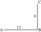
• 5.1. In the figure below three cities A, B and C are indicated with two roads between them.

There is no direct connection between cities A and C. The distance matrix between the three cities is:

$$ \left(\begin{array}{ccc}\hfill 0\hfill & \hfill 12\hfill & \hfill 21\hfill \\ {}\hfill 12\hfill & \hfill 0\hfill & \hfill 9\hfill \\ {}\hfill 21\hfill & \hfill 9\hfill & \hfill 0\hfill \end{array}\right) $$

• (a) Copy the figure and add the distances to the roads.

• (b) A direct (straight) road between cities A and C is built: how does the distance matrix change?

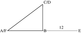
• (c) There are also three public parks D, E and F in the area. The (shortest) distance matrix between the cities (rows) and the parks (columns) is given by:

$$ \left(\begin{array}{ccc}\hfill 15\hfill & \hfill 24\hfill & \hfill 0\hfill \\ {}\hfill 9\hfill & \hfill 12\hfill & \hfill 12\hfill \\ {}\hfill 0\hfill & \hfill 15\hfill & \hfill 15\hfill \end{array}\right) $$

Indicate the location of the parks in the figure, assuming that the new road between A and C has been built.

• 5.2. Add and subtract (i.e. first-second matrix) the following pairs of matrices:

  • (a) $\left(\begin{array}{cc}\hfill 3\hfill & \hfill 4\hfill \\ {}\hfill -1\hfill & \hfill 8\hfill \end{array}\right)$ and $\left(\begin{array}{cc}\hfill 2\hfill & \hfill -2\hfill \\ {}\hfill 3\hfill & \hfill 7\hfill \end{array}\right)$

  • (b) $\left(\begin{array}{ccc}\hfill 3\hfill & \hfill -7\hfill & \hfill 4\hfill \\ {}\hfill -2\hfill & \hfill 6\hfill & \hfill 5\hfill \\ {}\hfill 1\hfill & \hfill -2\hfill & \hfill -9\hfill \end{array}\right)$ and $\left(\begin{array}{ccc}\hfill 4\hfill & \hfill 3\hfill & \hfill 2\hfill \\ {}\hfill 1\hfill & \hfill -2\hfill & \hfill -4\hfill \\ {}\hfill -5\hfill & \hfill 8\hfill & \hfill 11\hfill \end{array}\right)$

  • (c) $\left(\begin{array}{c}\hfill 1.2\kern0.5em 3.2\kern0.5em -1.5\hfill \\ {}\hfill \begin{array}{ccc}\hfill 3.4\hfill & \hfill 2.3\hfill & \hfill -3.2\hfill \end{array}\hfill \end{array}\right)$ and $\left(\begin{array}{c}\hfill 0.8\kern0.5em -1.6\kern0.5em 0.5\hfill \\ {}\hfill \begin{array}{ccc}\hfill 1.7\hfill & \hfill -1.3\hfill & \hfill 1.2\hfill \end{array}\hfill \end{array}\right)$

• 5.3. Calculate

  • (a) $\left(\begin{array}{c}\hfill 1\hfill \\ {}\hfill 7\hfill \\ {}\hfill 1\hfill \end{array}\kern0.5em \begin{array}{c}\hfill 2\hfill \\ {}\hfill 1\hfill \\ {}\hfill 4\hfill \end{array}\right)+3\left(\begin{array}{cc}\hfill \begin{array}{c}\hfill 1\hfill \\ {}\hfill 0\hfill \\ {}\hfill 1\hfill \end{array}\hfill & \hfill \begin{array}{c}\hfill 0\hfill \\ {}\hfill 1\hfill \\ {}\hfill 0\hfill \end{array}\hfill \end{array}\right)-2\left(\begin{array}{cc}\hfill \begin{array}{c}\hfill -1\hfill \\ {}\hfill 0\hfill \\ {}\hfill -2\hfill \end{array}\hfill & \hfill \begin{array}{c}\hfill 1\hfill \\ {}\hfill 4\hfill \\ {}\hfill -3\hfill \end{array}\hfill \end{array}\right)$

  • (b) $-\left(\begin{array}{cc}\hfill 0.5\hfill & \hfill 3.1\hfill \\ {}\hfill 6.7\hfill & \hfill 2.4\hfill \end{array}\right)-2\left(\begin{array}{cc}\hfill 1\hfill & \hfill 0.7\hfill \\ {}\hfill 1.2\hfill & \hfill 0.7\hfill \end{array}\right)+1.5\left(\begin{array}{cc}\hfill 4\hfill & \hfill 3\hfill \\ {}\hfill 8\hfill & \hfill 3\hfill \end{array}\right)$

5.2.2 Matrix Multiplication and Matrices as Transformations

Matrix addition, subtraction and scalar multiplication are quite straightforward generalizations of the same operations on vectors. For multiplication, the story is a little different, although there is a close relation between matrix multiplication and the vector inner product. A matrix product is only well defined if the number of columns in the first matrix equals the number of rows in the second matrix. Suppose A is an m × n matrix and B is an n × p matrix, then the product AB is defined by:

$$ {(AB)}_{ij}=\sum \limits_{k=1}^n{a}_{ik}{b}_{kj} $$

If you look closer at this definition, multiplying two matrices turns out to entail repeated vector inner product calculations, e.g. the element in the third row and second column of the product is the inner product of the third row of the first matrix with the second column of the second matrix. Let’s work this out for one abstract and for one concrete example:

$$ \left(\begin{array}{c}\hfill {a}_{11}\hfill \\ {}\hfill {a}_{21}\hfill \end{array}\kern0.5em \begin{array}{c}\hfill {a}_{12}\hfill \\ {}\hfill {a}_{22}\hfill \end{array}\kern0.5em \begin{array}{c}\hfill {a}_{13}\hfill \\ {}\hfill {a}_{23}\hfill \end{array}\right)\left(\begin{array}{c}\hfill \begin{array}{cc}\hfill {b}_{11}\hfill & \hfill {b}_{12}\hfill \end{array}\hfill \\ {}\hfill \begin{array}{cc}\hfill {b}_{21}\hfill & \hfill {b}_{22}\hfill \end{array}\hfill \\ {}\hfill \begin{array}{cc}\hfill {b}_{31}\hfill & \hfill {b}_{32}\hfill \end{array}\hfill \end{array}\right)=\left(\begin{array}{cc}\hfill {a}_{11}{b}_{11}+{a}_{12}{b}_{21}+{a}_{13}{b}_{31}\hfill & \hfill {a}_{11}{b}_{12}+{a}_{12}{b}_{22}+{a}_{13}{b}_{32}\hfill \\ {}\hfill {a}_{21}{b}_{11}+{a}_{22}{b}_{21}+{a}_{23}{b}_{31}\hfill & \hfill {a}_{21}{b}_{12}+{a}_{22}{b}_{22}+{a}_{23}{b}_{32}\hfill \end{array}\right) $$

$$ \left(\begin{array}{ccc}\hfill 3\hfill & \hfill 4\hfill & \hfill 2\hfill \\ {}\hfill -2\hfill & \hfill -1\hfill & \hfill 0\hfill \\ {}\hfill 2\hfill & \hfill -3\hfill & \hfill 7\hfill \end{array}\right)\left(\begin{array}{c}\hfill 1\kern0.5em 2\hfill \\ {}\hfill \begin{array}{cc}\hfill 3\hfill & \hfill 4\hfill \end{array}\hfill \\ {}\hfill \begin{array}{cc}\hfill 5\hfill & \hfill 6\hfill \end{array}\hfill \end{array}\right)=\left(\begin{array}{c}\hfill \begin{array}{cc}\hfill 3\cdot 1+4\cdot 3+2\cdot 5\hfill & \hfill 3\cdot 2+4\cdot 4+2\cdot 6\hfill \end{array}\hfill \\ {}\hfill \begin{array}{cc}\hfill -2\cdot 1-1\cdot 3+0\cdot 5\hfill & \hfill -2\cdot 2-1\cdot 4+0\cdot 6\hfill \end{array}\hfill \\ {}\hfill \begin{array}{cc}\hfill 2\cdot 1-3\cdot 3+7\cdot 5\hfill & \hfill 2\cdot 2-3\cdot 4+7\cdot 6\hfill \end{array}\hfill \end{array}\right)=\left(\begin{array}{c}\hfill \begin{array}{cc}\hfill 25\hfill & \hfill 34\hfill \end{array}\hfill \\ {}\hfill \begin{array}{cc}\hfill -5\hfill & \hfill -8\hfill \end{array}\hfill \\ {}\hfill \begin{array}{cc}\hfill 28\hfill & \hfill 34\hfill \end{array}\hfill \end{array}\right) $$

Exercises

• 5.4. Which pairs of the following matrices could theoretically be multiplied with each other and in which order ? Write down all possible products.

  • A with order 2 × 3

  • B with order 3 × 4

  • C with order 3 × 3

  • D with order 4 × 2

• 5.5. What is the order (size) of the resulting matrix when multiplying two matrices of orders

  • (a) 2 × 3 and 3 × 7

  • (b) 2 × 2 and 2 × 1

  • (c) 1 × 9 and 9 × 1

• 5.6. Calculate whichever product is possible: AB, BA, none or both.

  • (a) A = $\left(\begin{array}{cc}\hfill 3\hfill & \hfill 4\hfill \\ {}\hfill -1\hfill & \hfill 8\hfill \end{array}\right)$, B = $\left(\begin{array}{cc}\hfill 2\hfill & \hfill -2\hfill \\ {}\hfill 3\hfill & \hfill 7\hfill \end{array}\right)$

  • (b) A = $\left(\begin{array}{c}\hfill 3\hfill \\ {}\hfill -2\hfill \\ {}\hfill 1\hfill \end{array}\kern0.5em \begin{array}{c}\hfill -7\hfill \\ {}\hfill 6\hfill \\ {}\hfill -2\hfill \end{array}\right)$, B = $\left(\begin{array}{ccc}\hfill 4\hfill & \hfill 3\hfill & \hfill 2\hfill \\ {}\hfill 1\hfill & \hfill -2\hfill & \hfill -4\hfill \\ {}\hfill -5\hfill & \hfill 8\hfill & \hfill 11\hfill \end{array}\right)$

  • (c) A = $\left(\begin{array}{c}\hfill 1.2\kern0.5em 3.2\kern0.5em -1.5\hfill \\ {}\hfill \begin{array}{ccc}\hfill 3.4\hfill & \hfill 2.3\hfill & \hfill -3.2\hfill \end{array}\hfill \end{array}\right)$, B = $\left(\begin{array}{c}\hfill 0.8\kern0.5em -1.6\kern0.5em 0.5\hfill \\ {}\hfill \begin{array}{ccc}\hfill 1.7\hfill & \hfill -1.3\hfill & \hfill 1.2\hfill \end{array}\hfill \end{array}\right)$

So far, we discussed matrix operations as operations on abstract entities. However, matrices are actually commonly used to represent (linear) transformations. What this entails can be easily demonstrated by showing the effect of the application of matrices on vectors. Application here means that the matrix and vector are multiplied. Let’s first illustrate this by an example. Consider a vector $\overrightarrow{p}=\left(\begin{array}{c}\hfill 3\hfill \\ {}\hfill 2\hfill \end{array}\right)$, a matrix $M=\left(\begin{array}{cc}\hfill 1\hfill & \hfill 2\hfill \\ {}\hfill 2\hfill & \hfill -2\hfill \end{array}\right)$ and its product ${\overrightarrow{p}}^{\prime }=M\overrightarrow{p}=\left(\begin{array}{cc}\hfill 1\hfill & \hfill 2\hfill \\ {}\hfill 2\hfill & \hfill -2\hfill \end{array}\right)\left(\begin{array}{c}\hfill 3\hfill \\ {}\hfill 2\hfill \end{array}\right)=\left(\begin{array}{c}\hfill 7\hfill \\ {}\hfill 2\hfill \end{array}\right)$ (see Fig. 5.2).

Fig. 5.2

Illustration of how vector $\overset{\rightharpoonup }{p}$ is transformed into vector ${\overset{\rightharpoonup }{p}}^{\prime }$ by matrix M (see main text).

First, observe that when we calculate $M\overrightarrow{p}$ another 2 × 1 vector results, since we multiply a 2 × 2 matrix and a 2 × 1 vector. Apparently, judging from Fig. 5.2, applying the matrix M to the vector $\overset{\rightharpoonup }{p}$ transforms the vector; it rotates it and changes its length. To understand this transformation, let’s see how this matrix transforms the two basis vectors of 2D space; $\left(\begin{array}{c}\hfill 1\hfill \\ {}\hfill 0\hfill \end{array}\right)$ and $\left(\begin{array}{c}\hfill 0\hfill \\ {}\hfill 1\hfill \end{array}\right)$. These two vectors are called basis vectors, because any vector $\left(\begin{array}{c}\hfill a\hfill \\ {}\hfill b\hfill \end{array}\right)$ in 2D space can be built from them by a linear combination as follows: $\left(\begin{array}{c}\hfill a\hfill \\ {}\hfill b\hfill \end{array}\right)=a\left(\begin{array}{c}\hfill 1\hfill \\ {}\hfill 0\hfill \end{array}\right)+b\left(\begin{array}{c}\hfill 0\hfill \\ {}\hfill 1\hfill \end{array}\right)$. The matrix M transforms the first basis vector $\left(\begin{array}{c}\hfill 1\hfill \\ {}\hfill 0\hfill \end{array}\right)$ to $\left(\begin{array}{c}\hfill 1\hfill \\ {}\hfill 2\hfill \end{array}\right)$ and the second basis vector $\left(\begin{array}{c}\hfill 0\hfill \\ {}\hfill 1\hfill \end{array}\right)$ to $\left(\begin{array}{c}\hfill 2\hfill \\ {}\hfill -2\hfill \end{array}\right)$, i.e. the two columns of the matrix M show how the transform affects the basis vectors. The effect of M on any vector $\left(\begin{array}{c}\hfill a\hfill \\ {}\hfill b\hfill \end{array}\right)$ is thus equal to $M\left(\begin{array}{c}\hfill a\hfill \\ {}\hfill b\hfill \end{array}\right)=a\left(\begin{array}{c}\hfill 1\hfill \\ {}\hfill 2\hfill \end{array}\right)+b\left(\begin{array}{c}\hfill 2\hfill \\ {}\hfill -2\hfill \end{array}\right)$. For the example in Fig. 5.2 this results indeed in $M\left(\begin{array}{c}\hfill 3\hfill \\ {}\hfill 2\hfill \end{array}\right)=3\left(\begin{array}{c}\hfill 1\hfill \\ {}\hfill 2\hfill \end{array}\right)+2\left(\begin{array}{c}\hfill 2\hfill \\ {}\hfill -2\hfill \end{array}\right)=\left(\begin{array}{c}\hfill 7\hfill \\ {}\hfill 2\hfill \end{array}\right)$.

There are some special geometric transformation matrices, both in 2D, as well as 3D. One that is often encountered is the rotation matrix, that leaves the length of a vector unaltered, but rotates it around the origin in 2D or 3D. The rotation matrix has applications in e.g., the study of rigid body movements and in the manipulation of images, as in the preprocessing of functional magnetic resonance imaging (fMRI) scans. The transformation matrix that rotates a vector around the origin (in 2D) over an angle θ (counter clockwise) is given by $\left(\begin{array}{cc}\hfill \cos \theta \hfill & \hfill -\sin \theta \hfill \\ {}\hfill \sin \theta \hfill & \hfill \cos \theta \hfill \end{array}\right)$, as illustrated in Fig. 5.3 (cf. Chap. 3 on the geometrical definition of sine and cosine).

Fig. 5.3

Illustration of how the 2D basis vectors, $\left(\begin{array}{c}\hfill 1\hfill \\ {}\hfill 0\hfill \end{array}\right)$ in red and $\left(\begin{array}{c}\hfill 0\hfill \\ {}\hfill 1\hfill \end{array}\right)$ in blue, are affected by a counter-clockwise rotation over an angle θ. The vectors before rotation are indicated by drawn arrows, the vectors after rotation are indicated by dotted arrows.

Another common geometric transformation matrix is the shearing matrix, that transforms a square in 2D into a parallelogram (see Fig. 5.4). Applying the matrix transformation $\left(\begin{array}{cc}\hfill 1\hfill & \hfill k\hfill \\ {}\hfill 0\hfill & \hfill 1\hfill \end{array}\right)$ results in shearing along the x-axis (y-coordinate remains unchanged), whereas applying the matrix transformation $\left(\begin{array}{cc}\hfill 1\hfill & \hfill 0\hfill \\ {}\hfill k\hfill & \hfill 1\hfill \end{array}\right)$ results in shearing along the y-axis (x-coordinate remains unchanged). This transformation matrix is also applied in e.g., the preprocessing of fMRI scans.

Fig. 5.4

Illustration of how the two 2D basis vectors are affected by shearing along the x- and y-axes. The applied transformation matrix for shearing along the x-axis is $\left(\begin{array}{cc}\hfill 1\hfill & \hfill 3\hfill \\ {}\hfill 0\hfill & \hfill 1\hfill \end{array}\right)$ (results in red) and the applied transformation matrix for shearing along the y-axis is $\left(\begin{array}{cc}\hfill 1\hfill & \hfill 0\hfill \\ {}\hfill 2\hfill & \hfill 1\hfill \end{array}\right)$ (results in blue).

5.2.3 Alternative Matrix Multiplication

Just as there are different ways of multiplying vectors, there are also different ways of multiplying matrices, that are less common, however. For example, matrices can be multiplied element-wise; this product is also referred to as the Hadamard product , Schur product or pointwise product:

$$ {\left(A\circ B\right)}_{ij}={a}_{ij}{b}_{ij} $$

This only works when the two matrices have the same size. Another matrix product is the Kronecker product , which is a generalization of the tensor product (or dyadic product) for vectors. For vectors this product is equal to an n × 1 column vector being multiplied by a 1 × n row vector, which results in an n × n matrix when following the standard multiplication rules for matrices:

$$ \overrightarrow{a}\otimes \overrightarrow{b}={\overrightarrow{a}\overrightarrow{b}}^T=\left(\begin{array}{c}\hfill {a}_1\hfill \\ {}\hfill {a}_2\hfill \\ {}\hfill \vdots \hfill \\ {}\hfill {a}_n\hfill \end{array}\right)\left({b}_1\kern0.5em {b}_2\kern0.5em \cdots \kern0.5em {b}_n\right)=\left(\begin{array}{cccc}\hfill {a}_1{b}_1\hfill & \hfill {a}_1{b}_2\hfill & \hfill \cdots \hfill & \hfill {a}_1{b}_n\hfill \\ {}\hfill {a}_2{b}_1\hfill & \hfill {a}_2{b}_2\hfill & \hfill \cdots \hfill & \hfill {a}_2{b}_n\hfill \\ {}\hfill \vdots \hfill & \hfill \vdots \hfill & \hfill \ddots \hfill & \hfill \vdots \hfill \\ {}\hfill {a}_n{b}_1\hfill & \hfill {a}_n{b}_2\hfill & \hfill \cdots \hfill & \hfill {a}_n{b}_n\hfill \end{array}\right) $$

For two matrices A (m × n) and B (p × q), the Kronecker product A⊗B is defined by:

$$ A\otimes B=\left(\begin{array}{cccc}\hfill {a}_{11}B\hfill & \hfill {a}_{12}B\hfill & \hfill \cdots \hfill & \hfill {a}_{1n}B\hfill \\ {}\hfill {a}_{21}B\hfill & \hfill {a}_{22}B\hfill & \hfill \cdots \hfill & \hfill {a}_{2n}B\hfill \\ {}\hfill \vdots \hfill & \hfill \vdots \hfill & \hfill \ddots \hfill & \hfill \vdots \hfill \\ {}\hfill {a}_{m1}B\hfill & \hfill {a}_{m2}B\hfill & \hfill \cdots \hfill & \hfill {a}_{mn}B\hfill \end{array}\right) $$

Note that the size of the matrices A and B does not need to match for the Kronecker product . The Kronecker product has proven its use in the study of matrix theory (linear algebra), e.g. in solving matrix equations such as the Sylvester equation AX + XB = C for general A, B and C (see e.g. Horn and Johnson 1994).

Exercises

• 5.7. Calculate the Hadamard or pointwise product of

  • (a) $\left(\begin{array}{cc}\hfill 1\hfill & \hfill 2\hfill \\ {}\hfill -1\hfill & \hfill 1\hfill \end{array}\right)$ and $\left(\begin{array}{cc}\hfill 2\hfill & \hfill 3\hfill \\ {}\hfill 4\hfill & \hfill 1\hfill \end{array}\right)$

  • (b) $\left(\begin{array}{c}\hfill 2\kern0.5em -0.3\kern0.5em 1\hfill \\ {}\hfill \begin{array}{ccc}\hfill 1.5\hfill & \hfill 7\hfill & \hfill -0.4\hfill \end{array}\hfill \end{array}\right)$ and $\left(\begin{array}{c}\hfill 1.4\kern0.5em 9\kern0.5em 0.5\hfill \\ {}\hfill \begin{array}{ccc}\hfill 8\hfill & \hfill -0.1\hfill & \hfill 10\hfill \end{array}\hfill \end{array}\right)$

• 5.8. Calculate the Kronecker product of

  • (a) $\left(\begin{array}{cc}\hfill 1\hfill & \hfill 2\hfill \\ {}\hfill -1\hfill & \hfill 1\hfill \end{array}\right)$ and $\left(3\kern0.5em -1\kern0.5em 4\right)$

  • (b) $\left(-2\kern0.5em -3\right)$ and $\left(\begin{array}{ccc}\hfill 0\hfill & \hfill 1\hfill & \hfill 2\hfill \\ {}\hfill 3\hfill & \hfill 4\hfill & \hfill 5\hfill \\ {}\hfill 6\hfill & \hfill 7\hfill & \hfill 8\hfill \end{array}\right)$

5.2.4 Special Matrices and Other Basic Matrix Operations

There are some special forms of matrices and other basic operations on matrices that should be known before we can explain more interesting examples and applications of matrices.

The identity or unit matrix of size n is a square matrix of size n × n with ones on the diagonal and zeroes elsewhere. It is often referred to as I or, if necessary to explicitly mention its size, as I _n . The identity matrix is a special diagonal matrix . More generally, a diagonal matrix only has non-zero elements on the diagonal and zeroes elsewhere. If a diagonal matrix is extended with non-zero elements only above or only below the diagonal, we speak about an upper or lower triangular matrix , respectively. A matrix that is symmetric around the diagonal, i.e. for which a _ij  = a _ji , is called symmetric. An example of a symmetric matrix is a distance matrix, such as encountered in the very first example in this chapter. A matrix is skew-symmetric if a _ij  =  − a _ji . A matrix is called sparse if most of its elements are zero. In contrast, a matrix whose elements are almost all non-zero is called dense. A logical matrix (or binary or Boolean) matrix only contains zeroes and ones.

One operation that was already encountered in the previous chapter on vectors is the transpose. The transpose of an n × m matrix A is an m × n matrix of which the elements are defined as:

$$ {\left({A}^T\right)}_{ij}={a}_{ji} $$

A generalization of the transpose to complex-valued elements is the conjugate transpose , for which the elements are defined by:

$$ {\left({A}^{\ast}\right)}_{ij}={\overline{a}}_{ji}, $$

where the overbar indicates the complex conjugate (see Sect. 1.2.4.1). For real matrices, the transpose is equal to the conjugate transpose . In quantum mechanics the conjugate transpose is indicated by † (dagger) instead of *. Notice that (AB)^T = B ^T A ^T and (AB)^* = B ^* A ^* for matrices A and B for which the matrix product AB is possible.

Now that we have introduced the conjugate transpose , we can also introduce a few more special (complex) matrices. For a Hermitian matrix : A = A*, for a normal matrix : A*A = AA* and for a unitary matrix : AA* = I. Note that all unitary and Hermitian matrices are normal, but the reverse is not true. The unitary matrices will return when we explain singular value decomposition in Sect. 5.3.3.

All special matrices that were introduced in this section are summarized in Table 5.1 with their abstract definition and a concrete example.

Table 5.1 Special matrices with their abstract definition and an example

Exercises

• 5.9. In what sense (according to the definitions in Table 5.1) are the following matrices special? Mention at least one property.

  • (a) $\left(\begin{array}{ccc}\hfill 1\hfill & \hfill 1\hfill & \hfill 0\hfill \\ {}\hfill 1\hfill & \hfill 1\hfill & \hfill 0\hfill \\ {}\hfill 0\hfill & \hfill 0\hfill & \hfill 1\hfill \end{array}\right)$

  • (b) $\left(\begin{array}{ccc}\hfill 1\hfill & \hfill 0\hfill & \hfill 3\hfill \\ {}\hfill 0\hfill & \hfill 0\hfill & \hfill 0\hfill \\ {}\hfill 0\hfill & \hfill 0\hfill & \hfill 1\hfill \end{array}\right)$

  • (c) $\left(\begin{array}{ccc}\hfill 0\hfill & \hfill 4\hfill & \hfill 3\hfill \\ {}\hfill -4\hfill & \hfill 0\hfill & \hfill -7\hfill \\ {}\hfill -3\hfill & \hfill 7\hfill & \hfill 0\hfill \end{array}\right)$

  • (d) $\left(\begin{array}{ccc}\hfill 1\hfill & \hfill 4\hfill & \hfill 3\hfill \\ {}\hfill 0\hfill & \hfill 1\hfill & \hfill -7\hfill \\ {}\hfill 0\hfill & \hfill 0\hfill & \hfill 1\hfill \end{array}\right)$

  • (e) $\left(\begin{array}{ccc}\hfill 1\hfill & \hfill 0\hfill & \hfill 0\hfill \\ {}\hfill 0\hfill & \hfill 23\hfill & \hfill 0\hfill \\ {}\hfill 0\hfill & \hfill 0\hfill & \hfill -7\hfill \end{array}\right)$

  • (f) $\left(\begin{array}{ccc}\hfill 1\hfill & \hfill 0\hfill & \hfill 0\hfill \\ {}\hfill 0\hfill & \hfill 1\hfill & \hfill 0\hfill \\ {}\hfill 0\hfill & \hfill 0\hfill & \hfill 1\hfill \end{array}\right)$

• 5.10. Determine the conjugate transpose of

  • (a) $\left(\begin{array}{ccc}\hfill 1\hfill & \hfill 2\hfill & \hfill 3\hfill \\ {}\hfill -i\hfill & \hfill 1\hfill & \hfill -3-2i\hfill \\ {}\hfill 5\hfill & \hfill 4+5i\hfill & \hfill 3\hfill \end{array}\right)$

  • (b) $\left(\begin{array}{ccc}\hfill 1\hfill & \hfill 2\hfill & \hfill 3\hfill \\ {}\hfill -1\hfill & \hfill 1\hfill & \hfill -3\hfill \\ {}\hfill 5\hfill & \hfill 4\hfill & \hfill 0\hfill \end{array}\right)$

  • (c) $\left(\begin{array}{ccc}\hfill 4\hfill & \hfill 0\hfill & \hfill 3-2i\hfill \\ {}\hfill 19+i\hfill & \hfill -3\hfill & \hfill -3\hfill \\ {}\hfill -8i\hfill & \hfill -11-i\hfill & \hfill 17\hfill \end{array}\right)$

5.3 More Advanced Matrix Operations and Their Applications

Now that the basics of matrix addition, subtraction, scalar multiplication and multiplication hold no more secrets for you, it is time to get into more interesting mathematical concepts that rest on matrix calculus and to illustrate their applications.

5.3.1 Inverse and Determinant

One of the oldest applications of matrices is to solve systems of linear equations that were introduced to you in Chap. 2. Consider the following system of linear equations with three unknowns x, y and z:

$$ {\displaystyle \begin{array}{l}3x+4y-2z=5\\ {}-2x-2y+z=-3\\ {}x+y-7z=-18\end{array}} $$

This system can also be written as a matrix equation:

$\left(\begin{array}{ccc}\hfill 3\hfill & \hfill 4\hfill & \hfill -2\hfill \\ {}\hfill -2\hfill & \hfill -2\hfill & \hfill 1\hfill \\ {}\hfill 1\hfill & \hfill 1\hfill & \hfill -7\hfill \end{array}\right)\left(\begin{array}{c}\hfill x\hfill \\ {}\hfill y\hfill \\ {}\hfill z\hfill \end{array}\right)=\left(\begin{array}{c}\hfill 5\hfill \\ {}\hfill -3\hfill \\ {}\hfill -18\hfill \end{array}\right)$ or as

$M\left(\begin{array}{c}\hfill x\hfill \\ {}\hfill y\hfill \\ {}\hfill z\hfill \end{array}\right)=\left(\begin{array}{c}\hfill 5\hfill \\ {}\hfill -3\hfill \\ {}\hfill -18\hfill \end{array}\right)$ where $M=\left(\begin{array}{ccc}\hfill 3\hfill & \hfill 4\hfill & \hfill -2\hfill \\ {}\hfill -2\hfill & \hfill -2\hfill & \hfill 1\hfill \\ {}\hfill 1\hfill & \hfill 1\hfill & \hfill -7\hfill \end{array}\right)$

Such a system and more generally, systems of n equations in n unknowns, can be solved by using determinants, which is actually similar to using the inverse of a matrix to calculate the solution to a system of linear equations. The inverse of a square matrix A is the matrix A ⁻¹ such that AA ⁻¹ = A ⁻¹ A = I. The inverse of a matrix A does not always exist; if it does A is called invertable. Notice that (AB) ⁻¹ = B ⁻¹ A ⁻¹ for square , invertable matrices A and B. Now suppose that the matrix M in the matrix equation above has an inverse M ⁻¹. In that case, the solution to the equation would be given by:

$$ \left(\begin{array}{c}\hfill x\hfill \\ {}\hfill y\hfill \\ {}\hfill z\hfill \end{array}\right)=I\left(\begin{array}{c}\hfill x\hfill \\ {}\hfill y\hfill \\ {}\hfill z\hfill \end{array}\right)={M}^{-1}M\left(\begin{array}{c}\hfill x\hfill \\ {}\hfill y\hfill \\ {}\hfill z\hfill \end{array}\right)={M}^{-1}\left(\begin{array}{c}\hfill 5\hfill \\ {}\hfill -3\hfill \\ {}\hfill -18\hfill \end{array}\right) $$

Mathematically, the inverse of 2 × 2 matrix $\left(\begin{array}{cc}\hfill a\hfill & \hfill b\hfill \\ {}\hfill c\hfill & \hfill d\hfill \end{array}\right)$ is given by $\frac{1}{ad- bc}\left(\begin{array}{cc}\hfill d\hfill & \hfill -b\hfill \\ {}\hfill -c\hfill & \hfill a\hfill \end{array}\right)$ where ad − bc is the determinant $\left|\begin{array}{cc}\hfill a\hfill & \hfill b\hfill \\ {}\hfill c\hfill & \hfill d\hfill \end{array}\right|$ of the matrix. This illustrates why a square matrix has an inverse if and only if (iff) its determinant is not zero, as division by zero would result in infinity. For a 3 × 3 matrix or higher-dimensional matrices the inverse can still be calculated by hand, but it quickly becomes cumbersome. In general, for a matrix A:

$$ {A}^{-1}=\frac{1}{\det (A)} adj(A), $$

where adj(A) is the adjoint of A. The adjoint of a matrix A is the transpose of the cofactor matrix. Each (i,j)-element of a cofactor matrix is given by the determinant of the matrix that remains when the i-th row and j-th column are removed, multiplied by −1 if i + j is odd. In Box 5.1 the inverse is calculated of the matrix M given in the example that we started this section with.

Box 5.1 Example of calculating the inverse of a matrix

To be able to calculate M ⁻¹ where $M=\left(\begin{array}{ccc}\hfill 3\hfill & \hfill 4\hfill & \hfill -2\hfill \\ {}\hfill -2\hfill & \hfill -2\hfill & \hfill 1\hfill \\ {}\hfill 1\hfill & \hfill 1\hfill & \hfill -7\hfill \end{array}\right)$ we first need to know how to calculate the determinant of a 3 × 3 matrix. This is done by first choosing a reference row or column and calculating the cofactors for that row or column. Then the determinant is equal to the sum of the products of the elements of that row or column with its cofactors. This sounds rather abstract so let’s calculate det(M) by taking its first row as a reference.

$$ {\displaystyle \begin{array}{l}\det (M)=\det \left(\begin{array}{ccc}\hfill 3\hfill & \hfill 4\hfill & \hfill -2\hfill \\ {}\hfill -2\hfill & \hfill -2\hfill & \hfill 1\hfill \\ {}\hfill 1\hfill & \hfill 1\hfill & \hfill -7\hfill \end{array}\right)\\ {}=3\left|\begin{array}{cc}\hfill -2\hfill & \hfill 1\hfill \\ {}\hfill 1\hfill & \hfill -7\hfill \end{array}\right|-4\left|\begin{array}{cc}\hfill -2\hfill & \hfill 1\hfill \\ {}\hfill 1\hfill & \hfill -7\hfill \end{array}\right|-2\left|\begin{array}{cc}\hfill -2\hfill & \hfill -2\hfill \\ {}\hfill 1\hfill & \hfill 1\hfill \end{array}\right|\\ {}=3\cdot 13-4\cdot 13-2\cdot 0=-13\end{array}} $$

For the matrix M its cofactor matrix is given by

$\left(\begin{array}{ccc}\hfill \left|\begin{array}{cc}\hfill -2\hfill & \hfill 1\hfill \\ {}\hfill 1\hfill & \hfill -7\hfill \end{array}\right|\hfill & \hfill -\left|\begin{array}{cc}\hfill -2\hfill & \hfill 1\hfill \\ {}\hfill 1\hfill & \hfill -7\hfill \end{array}\right|\hfill & \hfill \left|\begin{array}{cc}\hfill -2\hfill & \hfill -2\hfill \\ {}\hfill 1\hfill & \hfill 1\hfill \end{array}\right|\hfill \\ {}\hfill -\left|\begin{array}{cc}\hfill 4\hfill & \hfill -2\hfill \\ {}\hfill 1\hfill & \hfill -7\hfill \end{array}\right|\hfill & \hfill \left|\begin{array}{cc}\hfill 3\hfill & \hfill -2\hfill \\ {}\hfill 1\hfill & \hfill -7\hfill \end{array}\right|\hfill & \hfill -\left|\begin{array}{cc}\hfill 3\hfill & \hfill 4\hfill \\ {}\hfill 1\hfill & \hfill 1\hfill \end{array}\right|\hfill \\ {}\hfill \left|\begin{array}{cc}\hfill 4\hfill & \hfill -2\hfill \\ {}\hfill -2\hfill & \hfill 1\hfill \end{array}\right|\hfill & \hfill -\left|\begin{array}{cc}\hfill 3\hfill & \hfill -2\hfill \\ {}\hfill -2\hfill & \hfill 1\hfill \end{array}\right|\hfill & \hfill \left|\begin{array}{cc}\hfill 3\hfill & \hfill 4\hfill \\ {}\hfill -2\hfill & \hfill -2\hfill \end{array}\right|\hfill \end{array}\right)=\left(\begin{array}{ccc}\hfill 13\hfill & \hfill -13\hfill & \hfill 0\hfill \\ {}\hfill 26\hfill & \hfill -19\hfill & \hfill 1\hfill \\ {}\hfill 0\hfill & \hfill 1\hfill & \hfill 2\hfill \end{array}\right)$.Hence, the adjoint matrix of M is its transpose $\left(\begin{array}{ccc}\hfill 13\hfill & \hfill 26\hfill & \hfill 0\hfill \\ {}\hfill -13\hfill & \hfill -19\hfill & \hfill 1\hfill \\ {}\hfill 0\hfill & \hfill 1\hfill & \hfill 2\hfill \end{array}\right)$. Thus, the inverse of M is given by:

$$ {M}^{-1}=\frac{1}{-13}\left(\begin{array}{ccc}\hfill 13\hfill & \hfill 26\hfill & \hfill 0\hfill \\ {}\hfill -13\hfill & \hfill -19\hfill & \hfill 1\hfill \\ {}\hfill 0\hfill & \hfill 1\hfill & \hfill 2\hfill \end{array}\right) $$

To verify that the inverse that we calculated in Box 5.1 is correct, it suffices to verify that the matrix multiplied by its inverse equals the identity matrix. Thus, for matrix M we verify that M ⁻¹ M = I:

$$ {\displaystyle \begin{array}{l}{M}^{-1}M=\frac{1}{-13}\left(\begin{array}{ccc}\hfill 13\hfill & \hfill 26\hfill & \hfill 0\hfill \\ {}\hfill -13\hfill & \hfill -19\hfill & \hfill 1\hfill \\ {}\hfill 0\hfill & \hfill 1\hfill & \hfill 2\hfill \end{array}\right)\left(\begin{array}{ccc}\hfill 3\hfill & \hfill 4\hfill & \hfill -2\hfill \\ {}\hfill -2\hfill & \hfill -2\hfill & \hfill 1\hfill \\ {}\hfill 1\hfill & \hfill 1\hfill & \hfill -7\hfill \end{array}\right)\\ {}=-\frac{1}{13}\left(\begin{array}{ccc}\hfill -13\hfill & \hfill 0\hfill & \hfill 0\hfill \\ {}\hfill 0\hfill & \hfill -13\hfill & \hfill 0\hfill \\ {}\hfill 0\hfill & \hfill 0\hfill & \hfill -13\hfill \end{array}\right)=\left(\begin{array}{ccc}\hfill 1\hfill & \hfill 0\hfill & \hfill 0\hfill \\ {}\hfill 0\hfill & \hfill 1\hfill & \hfill 0\hfill \\ {}\hfill 0\hfill & \hfill 0\hfill & \hfill 1\hfill \end{array}\right)=I\end{array}} $$

Finally, now that we have found M ⁻¹, we can find the solution to the system of equations that we started with:

$$ \left(\begin{array}{c}\hfill x\hfill \\ {}\hfill y\hfill \\ {}\hfill z\hfill \end{array}\right)={M}^{-1}\left(\begin{array}{c}\hfill 5\hfill \\ {}\hfill -3\hfill \\ {}\hfill -18\hfill \end{array}\right)=-\frac{1}{13}\left(\begin{array}{ccc}\hfill 13\hfill & \hfill 26\hfill & \hfill 0\hfill \\ {}\hfill -13\hfill & \hfill -19\hfill & \hfill 1\hfill \\ {}\hfill 0\hfill & \hfill 1\hfill & \hfill 2\hfill \end{array}\right)\left(\begin{array}{c}\hfill 5\hfill \\ {}\hfill -3\hfill \\ {}\hfill -18\hfill \end{array}\right)=-\frac{1}{13}\left(\begin{array}{c}\hfill -13\hfill \\ {}\hfill -26\hfill \\ {}\hfill -39\hfill \end{array}\right)=\left(\begin{array}{c}\hfill 1\hfill \\ {}\hfill 2\hfill \\ {}\hfill 3\hfill \end{array}\right) $$

Finally, this solution can again be verified by inserting the solution in the system of equations that was given at the beginning of this section.

Cramer’s rule is an explicit formulation of using determinants to solve systems of linear equations. We first formulate it for a system of three linear equations in three unknowns

$$ {\displaystyle \begin{array}{l}{a}_1x+{b}_1y+{c}_1z={d}_1\\ {}{a}_2x+{b}_2y+{c}_2z={d}_2\\ {}{a}_3x+{b}_3y+{c}_3z={d}_3\end{array}} $$

Its associated determinant is:

$$ D=\left|\begin{array}{ccc}\hfill {a}_1\hfill & \hfill {b}_1\hfill & \hfill {c}_1\hfill \\ {}\hfill {a}_2\hfill & \hfill {b}_2\hfill & \hfill {c}_2\hfill \\ {}\hfill {a}_3\hfill & \hfill {b}_3\hfill & \hfill {c}_3\hfill \end{array}\right|. $$

We can also define the determinant

$$ {D}_x=\left|\begin{array}{ccc}\hfill {d}_1\hfill & \hfill {b}_1\hfill & \hfill {c}_1\hfill \\ {}\hfill {d}_2\hfill & \hfill {b}_2\hfill & \hfill {c}_2\hfill \\ {}\hfill {d}_3\hfill & \hfill {b}_3\hfill & \hfill {c}_3\hfill \end{array}\right|, $$

which is the determinant of the system’s associated matrix with its first column replaced by the vector of constants and similarly

$$ {D}_y=\left|\begin{array}{ccc}\hfill {a}_1\hfill & \hfill {d}_1\hfill & \hfill {c}_1\hfill \\ {}\hfill {a}_2\hfill & \hfill {d}_2\hfill & \hfill {c}_2\hfill \\ {}\hfill {a}_3\hfill & \hfill {d}_3\hfill & \hfill {c}_3\hfill \end{array}\right|\kern0.5em \mathrm{and}\kern0.5em {D}_z=\left|\begin{array}{ccc}\hfill {a}_1\hfill & \hfill {b}_1\hfill & \hfill {d}_1\hfill \\ {}\hfill {a}_2\hfill & \hfill {b}_2\hfill & \hfill {d}_2\hfill \\ {}\hfill {a}_3\hfill & \hfill {b}_3\hfill & \hfill {d}_3\hfill \end{array}\right|. $$

Then, x, y and z can be calculated as:

$$ x=\frac{D_x}{D},y=\frac{D_y}{D},z=\frac{D_z}{D}. $$

Similarly, the solution of a system of n linear equations in n unknowns:

$$ \left(\begin{array}{cccc}\hfill {a}_{11}\hfill & \hfill {a}_{12}\hfill & \hfill \cdots \hfill & \hfill {a}_{1n}\hfill \\ {}\hfill {a}_{21}\hfill & \hfill {a}_{22}\hfill & \hfill \cdots \hfill & \hfill {a}_{2n}\hfill \\ {}\hfill \vdots \hfill & \hfill \vdots \hfill & \hfill \ddots \hfill & \hfill \vdots \hfill \\ {}\hfill {a}_{n1}\hfill & \hfill {a}_{n2}\hfill & \hfill \cdots \hfill & \hfill {a}_{nn}\hfill \end{array}\right)\left(\begin{array}{c}\hfill {x}_1\hfill \\ {}\hfill {x}_2\hfill \\ {}\hfill \vdots \hfill \\ {}\hfill {x}_n\hfill \end{array}\right)=\left(\begin{array}{c}\hfill {b}_1\hfill \\ {}\hfill {b}_2\hfill \\ {}\hfill \vdots \hfill \\ {}\hfill {b}_n\hfill \end{array}\right)\kern0.5em \mathrm{or}\kern0.5em Ax=b, $$

according to Cramer’s rule is given by:

${x}_1=\frac{D_{x_1}}{D},{x}_2=\frac{D_{x_2}}{D},\kern0.5em \dots \kern0.5em ,{x}_n=\frac{D_{x_n}}{D}$, where ${D}_{x_i}$ is the determinant of the matrix formed by replacing the i-th column of A by the column vector $\overset{\rightharpoonup }{b}$. Note that Cramer’s rule only applies when D ≠ 0. Unfortunately, Cramer’s rule is computationally very inefficient for larger systems and thus not often used in practice.

Exercises

• 5.11. Show that using Cramer’s rule to find the solution to a system of two linear equations in two unknowns ax + by = c and dx + ey = f is the same as applying the inverse of the matrix $\left(\begin{array}{cc}\hfill a\hfill & \hfill b\hfill \\ {}\hfill d\hfill & \hfill e\hfill \end{array}\right)$ to the vector $\left(\begin{array}{c}\hfill c\hfill \\ {}\hfill f\hfill \end{array}\right)$.

• 5.12. Find the solution to the following systems of linear equations using Cramer’s rule :

  • (a) (Example 2.6) 3x + 5 = 5y ∧ 2x − 5y = 6

  • (b) 4x − 2y − 2z = 10 ∧ 2x + 8y + 4z = 32 ∧ 30x + 12y − 4z = 24

• 5.13. Find the solution to the following systems of linear equations using the matrix inverse:

  • (a) (Exercise 2.4a) $x-2y=4\wedge \frac{x}{3}-y=\frac{4}{3}$

  • (b) (Example 2.7) 2x + y + z = 4 ∧ x − 7 − 2y =  − 3z ∧ 2y + 10 − 2z = 3x

Now that you know how to calculate the determinant of a matrix, it is easy to recognize that the algebraic definition of the cross-product introduced in Sect. 4.2.2.2 is similar to calculating the determinant of a very special matrix:

$$ {\displaystyle \begin{array}{l}\overrightarrow{a}\times \overrightarrow{b}=\left(\begin{array}{c}\hfill {a}_1\hfill \\ {}\hfill {a}_2\hfill \\ {}\hfill {a}_3\hfill \end{array}\right)\times \left(\begin{array}{c}\hfill {b}_1\hfill \\ {}\hfill {b}_2\hfill \\ {}\hfill {b}_3\hfill \end{array}\right)=\left(\begin{array}{c}\hfill {a}_2{b}_3-{a}_3{b}_2\hfill \\ {}\hfill {a}_3{b}_1-{a}_1{b}_3\hfill \\ {}\hfill {a}_1{b}_2-{a}_2{b}_1\hfill \end{array}\right)=\left|\begin{array}{ccc}\hfill \overrightarrow{i}\hfill & \hfill \overrightarrow{j}\hfill & \hfill \overrightarrow{k}\hfill \\ {}\hfill {a}_1\hfill & \hfill {a}_2\hfill & \hfill {a}_3\hfill \\ {}\hfill {b}_1\hfill & \hfill {b}_2\hfill & \hfill {b}_3\hfill \end{array}\right|\\ {}=\left|\begin{array}{cc}\hfill {a}_2\hfill & \hfill {a}_3\hfill \\ {}\hfill {b}_2\hfill & \hfill {b}_3\hfill \end{array}\right|\overrightarrow{i}-\left|\begin{array}{cc}\hfill {a}_1\hfill & \hfill {a}_3\hfill \\ {}\hfill {b}_1\hfill & \hfill {b}_3\hfill \end{array}\right|\overrightarrow{j}+\left|\begin{array}{cc}\hfill {a}_1\hfill & \hfill {a}_2\hfill \\ {}\hfill {b}_1\hfill & \hfill {b}_2\hfill \end{array}\right|\overrightarrow{k}\end{array}} $$

Finding the inverse of larger square matrices and thus finding the solution to larger systems of linear equations may also be accomplished by calculating the inverse matrix by hand. However, as you will surely have noticed when doing the exercises, finding the solution of a system of three linear equations with three unknowns calculating the inverse matrix by hand is already rather cumbersome, tedious and error-prone. Computers do a much better job than we at this sort of task which is why (numerical) mathematicians have developed clever, fast computer algorithms to determine matrix inverses. There is even a whole branch of numerical mathematics that focuses on solving systems of equations that can be represented by sparse matrices, as fast as possible (Saad 2003). The relevance of sparse matrices is that they naturally appear in many scientific or engineering applications whenever partial differential equations (see Box 5.2 and Chap. 6) are numerically solved on a grid. Typically, only local physical interactions play a role in such models of reality and thus only neighboring grid cells interact, resulting in sparse matrices. Examples are when heat dissipation around an underground gas tube or turbulence in the wake of an airfoil needs to be simulated. In Box 5.2 a simple example is worked out to explain how a discretized partial differential equation can result in a sparse matrix.

Box 5.2 How discretizing a partial differential equation can yield a sparse matrix

We here consider the Laplace equation for a scalar function u in two dimensions (indicated by x and y), which is e.g. encountered in the fields of electromagnetism and fluid dynamics:

$$ {\nabla}^2u=\frac{\partial^2u}{\partial {x}^2}+\frac{\partial^2u}{\partial {y}^2}=0 $$

It can describe airflow around airfoils or water waves, under specific conditions. In Sect. 6.11 partial derivatives are explained in more detail. To solve this equation on a rectangle, a grid or lattice of evenly spaced points (with distance h) can be overlaid as in Fig. 5.5.

Fig. 5.5

Grid with equal spacing h for numerical solution of the Laplace equation in two dimensions. To solve for the point (i,j) (in red), values in the surrounding points (in blue) can be used.

One method to discretize the Laplace equation on this grid (see for details e.g. Press et al. n.d.) is:

$$ \frac{u_{i-1,j}-2{u}_{i,j}+{u}_{i+1,j}}{h^2}+\frac{u_{i,j-1}-2{u}_{i,j}+{u}_{i,j+1}}{h^2}=0 $$

or

$$ {u}_{i.j}=\frac{1}{4}\left({u}_{i-1,j}+{u}_{i+1,j}+{u}_{i,j-1}+{u}_{i,j+1}\right) $$

(5.1)

Here, i runs over the grid cells in x-direction and j runs over the grid cells in y-direction. This discretized equation already shows that the solution in a point (i,j) (in red in the figure) is only determined by the values in its local neighbours, i.e. the four points (i + 1,j), (i − 1,j), (i, j + 1) and (i, j − 1) (in blue in the figure) directly surrounding it. There are alternative discretizations that use variable spacings in the two grid directions and/or fewer or more points; the choice is determined by several problem parameters such as the given boundary conditions.

Here, I only want to illustrate how solving this problem involves a sparse matrix. Typically, iterative solution methods are used, meaning that the solution is approximated step-by-step starting from an initial solution and adapting the solution at every iteration until the solution hardly changes anymore. The solution at iteration step n + 1 (indicated by a superscript) can then be derived from the solution at time step n e.g. as follows (cf. Eq. 5.1):

$$ {u}_{i,j}^{n+1}=\frac{1}{4}\left({u}_{i-1,j}^n+{u}_{i+1,j}^n+{u}_{i,j-1}^n+{u}_{i,j+1}^n\right) $$

Here, we can recognize a (sparse ) matrix transformation as I will explain now. Suppose we are dealing with the 11 × 7 grid in the figure. We can then arrange the values of u at iteration step n in a vector e.g. by row: ${\overrightarrow{u}}^n={\left(\begin{array}{ccc}\hfill {u}_{1,1}^n\hfill & \hfill \cdots \hfill & \hfill {u}_{1,11}^n\hfill \end{array}\kern0.5em \begin{array}{ccc}\hfill {u}_{2,1}^n\hfill & \hfill \cdots \hfill & \hfill {u}_{2,11}^n\hfill \end{array}\kern0.5em \begin{array}{ccc}\hfill {u}_{3,1}^n\hfill & \hfill \cdots \hfill & \hfill {u}_{7,11}^n\hfill \end{array}\right)}^T$ and similarly for the values of u at iteration step n + 1. The 77 × 77 matrix transforming ${\overrightarrow{u}}^n$ into ${\overrightarrow{u}}^{n+1}$ then has only four non-zero entries and 73 zeroes in every row (with some exceptions for the treatment of the boundary grid points) and is thus sparse . It should be noted that this particular iterative solution method is slow and that much faster methods are available.

5.3.2 Eigenvectors and Eigenvalues

A first mathematical concept that rests on matrix calculus and that is part of other interesting matrix decomposition methods (see Sect. 5.3.3) is that of eigenvectors and eigenvalues. An eigenvector $\overrightarrow{v}$ of a square matrix M is a non-zero column vector that does not change its orientation (although it may change its length by a factor λ) as a result of the transformation represented by the matrix. In mathematical terms:

$$ M\overrightarrow{v}=\lambda \overrightarrow{v}, $$

where λ is a scalar known as the eigenvalue. Eigenvectors and eigenvalues have many applications, of which we will encounter a few in the next section. For example, they allow to determine the principal axes of rotational movements of rigid bodies (dating back to eighteenth century Euler), to find common features in images as well as statistical data reduction.

To find the eigenvectors of a matrix M, the following system of linear equations has to be solved:

$$ \left(M-\lambda I\right)\overrightarrow{v}=0. $$

It is known that this equation has a solution iff the determinant of M − λI is zero. Thus, the eigenvalues of M are those values of λ that satisfy |M − λI| = 0. This determinant is a polynomial in λ of which the highest power is the order of the matrix M. The eigenvalues can be found by finding the roots of this polynomial, known as the characteristic polynomial of M. There are as many roots as the order (highest power) of the polynomial. Once the eigenvalues are known, the related eigenvectors can be found by solving for $\overrightarrow{v}$ in $M\overrightarrow{v}=\lambda \overrightarrow{v}$. This probably sounds quite abstract, so a concrete example is given in Box 5.3.

Box 5.3 Example of calculating the eigenvalues and eigenvectors of a matrix

To find the eigenvalues of the matrix $\left(\begin{array}{cc}\hfill 3\hfill & \hfill 1\hfill \\ {}\hfill 2\hfill & \hfill 4\hfill \end{array}\right)$, we first determine its characteristic equation as the determinant

$$ \left|\left(\begin{array}{cc}\hfill 3\hfill & \hfill 1\hfill \\ {}\hfill 2\hfill & \hfill 4\hfill \end{array}\right)-\lambda \left(\begin{array}{cc}\hfill 1\hfill & \hfill 0\hfill \\ {}\hfill 0\hfill & \hfill 1\hfill \end{array}\right)\right|=\left|\left(\begin{array}{cc}\hfill 3-\lambda \hfill & \hfill 1\hfill \\ {}\hfill 2\hfill & \hfill 4-\lambda \hfill \end{array}\right)\right|=\left(3-\lambda \right)\left(4-\lambda \right)-2={\lambda}^2-7\lambda +10 $$

Since λ ² − 7λ + 10 = (λ − 2)(λ − 5), the roots of this polynomial are given by λ = 2 and λ = 5. The eigenvector for λ = 2 follows from:

$$ {\displaystyle \begin{array}{l}\left(\begin{array}{cc}\hfill 3\hfill & \hfill 1\hfill \\ {}\hfill 2\hfill & \hfill 4\hfill \end{array}\right)\left(\begin{array}{c}\hfill x\hfill \\ {}\hfill y\hfill \end{array}\right)=2\left(\begin{array}{c}\hfill x\hfill \\ {}\hfill y\hfill \end{array}\right)\Rightarrow \left(\begin{array}{c}\hfill 3x+y\hfill \\ {}\hfill 2x+4y\hfill \end{array}\right)=\left(\begin{array}{c}\hfill 2x\hfill \\ {}\hfill 2y\hfill \end{array}\right)\\ {}\Rightarrow 3x+y=2x\wedge 2x+4y=2y\\ {}\Rightarrow x+y=0\wedge 2x+2y=0\\ {}\Rightarrow x=-y\\ {}\Rightarrow \left(\begin{array}{c}\hfill x\hfill \\ {}\hfill y\hfill \end{array}\right)=\left(\begin{array}{c}\hfill -1\hfill \\ {}\hfill 1\hfill \end{array}\right)\end{array}} $$

Notice that $\left(\begin{array}{c}\hfill -1\hfill \\ {}\hfill 1\hfill \end{array}\right)$ is the eigenvector in this case, because for any multiple of this vector it is true that x = −y.

Similarly, the eigenvector for λ = 5 follows from:

$$ {\displaystyle \begin{array}{l}\left(\begin{array}{cc}\hfill 3\hfill & \hfill 1\hfill \\ {}\hfill 2\hfill & \hfill 4\hfill \end{array}\right)\left(\begin{array}{c}\hfill x\hfill \\ {}\hfill y\hfill \end{array}\right)=5\left(\begin{array}{c}\hfill x\hfill \\ {}\hfill y\hfill \end{array}\right)\Rightarrow \left(\begin{array}{c}\hfill 3x+y\hfill \\ {}\hfill 2x+4y\hfill \end{array}\right)=\left(\begin{array}{c}\hfill 5x\hfill \\ {}\hfill 5y\hfill \end{array}\right)\\ {}\Rightarrow 3x+y=5x\wedge 2x+4y=5y\\ {}\Rightarrow -2x+y=0\wedge 2x-y=0\\ {}\Rightarrow x=\frac{1}{2}y\\ {}\Rightarrow \left(\begin{array}{c}\hfill x\hfill \\ {}\hfill y\hfill \end{array}\right)=\left(\begin{array}{c}\hfill 1\hfill \\ {}\hfill 2\hfill \end{array}\right)\end{array}} $$

Notice that $\left(\begin{array}{c}\hfill 1\hfill \\ {}\hfill 2\hfill \end{array}\right)$ is the eigenvector in this case, because for any multiple of this vector it is true that 2x = y.

Hence, the matrix $\left(\begin{array}{cc}\hfill 3\hfill & \hfill 1\hfill \\ {}\hfill 2\hfill & \hfill 4\hfill \end{array}\right)$ has eigenvectors $\left(\begin{array}{c}\hfill -1\hfill \\ {}\hfill 1\hfill \end{array}\right)$ and $\left(\begin{array}{c}\hfill 1\hfill \\ {}\hfill 2\hfill \end{array}\right)$ with eigenvalues 2 and 5, respectively.

Exercises

• 5.14. Consider the shearing matrix $\left(\begin{array}{cc}\hfill 1\hfill & \hfill 2\hfill \\ {}\hfill 0\hfill & \hfill 1\hfill \end{array}\right)$. Without calculation, which are the eigenvectors of this matrix and why?

• 5.15. Calculate the eigenvectors and eigenvalues of

  • (a) $\left(\begin{array}{ccc}\hfill 7\hfill & \hfill 0\hfill & \hfill 0\hfill \\ {}\hfill 0\hfill & \hfill -19\hfill & \hfill 0\hfill \\ {}\hfill 0\hfill & \hfill 0\hfill & \hfill 2\hfill \end{array}\right)$

  • (b) $\left(\begin{array}{cc}\hfill 2\hfill & \hfill 1\hfill \\ {}\hfill -1\hfill & \hfill 4\hfill \end{array}\right)$

  • (c) $\left(\begin{array}{ccc}\hfill 2\hfill & \hfill 2\hfill & \hfill -1\hfill \\ {}\hfill 1\hfill & \hfill 3\hfill & \hfill -1\hfill \\ {}\hfill 1\hfill & \hfill 4\hfill & \hfill -2\hfill \end{array}\right)$

  • (d) $\left(\begin{array}{cc}\hfill 5\hfill & \hfill 1\hfill \\ {}\hfill 4\hfill & \hfill 5\hfill \end{array}\right)$

5.3.3 Diagonalization, Singular Value Decomposition, Principal Component Analysis and Independent Component Analysis

In the previous section I already alluded to several applications using eigenvalues and eigenvectors. In this section I will discuss some of the most well-known and most often used methods that employ eigendecomposition and that underlie these applications.

The simplest is diagonalization . A matrix M can be diagonalized if it can be written as

$$ M={VDV}^{-1} $$

(5.2)

where V is an invertible matrix and D is a diagonal matrix . First note that V has to be square to be invertible, so that M also has to be square to be diagonalizable. Now let’s find out how eigenvalues and eigenvectors play a role in Eq. 5.2. We can rewrite Eq. 5.2 by right multiplication with V to:

$$ MV= VD $$

or similarly, when we indicate the columns of V by ${\overrightarrow{v}}_i$ and the elements of D by d _i , i = 1, …, n, then:

$$ M\left({\overrightarrow{v}}_1\kern0.5em {\overrightarrow{v}}_2\kern0.5em \cdots \kern0.5em {\overrightarrow{v}}_n\right)=\left(\begin{array}{cccc}\hfill {\overrightarrow{v}}_1\hfill & \hfill {\overrightarrow{v}}_2\hfill & \hfill \cdots \hfill & \hfill {\overrightarrow{v}}_n\hfill \end{array}\right)D=\left({d}_1\begin{array}{cccc}\hfill {\overrightarrow{v}}_1\hfill & \hfill {d}_2{\overrightarrow{v}}_2\hfill & \hfill \cdots \hfill & \hfill {d}_n{\overrightarrow{v}}_n\hfill \end{array}\right) $$

This shows that in Eq. 5.2 the columns of V must be the eigenvectors of M and the diagonal elements of D must be the eigenvalues of M. We just noted that only square matrices can potentially be diagonalized. What singular value decomposition does is generalize the concept of diagonalization to any matrix, making it a very powerful method.

For an intuitive understanding of SVD you can think of a matrix as a large table of data, e.g. describing which books from a collection of 500 a 1000 people have read. In that case the matrix could contains ones for books (in 500 columns) that a particular reader (in 1000 rows) read and zeroes for the books that weren’t read. SVD can help summarize the data in this large matrix. When SVD is applied to this particular matrix it will help identify specific sets of books that are often read by the same readers. For example, SVD may find that all thrillers in the collection are often read together, or all science fiction novels, or all romantic books; the composition of these subcollections will be expressed in the singular vectors, and their importance in the singular values. Now each reader’s reading behavior can be expressed in a much more compact way than by just tabulating all books that he or she read. Instead, SVD allows to say e.g., that a reader is mostly interested in science fiction novels, or maybe that in addition, there is some interest in popular science books. Let’s see how this compression of data can be achieved by SVD by first looking at its mathematics .

In singular value decomposition (SVD) an m × n rectangular matrix M is decomposed into a product of three matrices as follows:

$$ M=U\Sigma {V}^{\ast } $$

where U is a unitary (see Table 5.1) m × m matrix, Σ an m × n diagonal matrix with non-negative real entries and V another unitary n × n matrix. To determine these matrices you have to calculate the sets of orthonormal eigenvectors of MM ^* and M ^* M. This can be done, as MM ^* and M ^* M are square . The orthonormal eigenvectors of the former are the columns of U and the orthonormal eigenvectors of the latter are the columns of V. The square roots of the non-zero eigenvalues of MM ^* or M ^* M (which do not differ) are the so-called singular values of M and form the diagonal elements of Σ in decreasing order, completed by zeroes if necessary. The columns of U are referred to as the left-singular vectors of M and the columns of V are referred to as the right-singular vectors of M. For an example which can also be intuitively understood, see Box 5.4.

Box 5.4 Example of SVD of a real square matrix and its intuitive understanding

To determine the SVD of the matrix $\mathbf{M}=\left(\begin{array}{cc}\hfill 1\hfill & \hfill -2\hfill \\ {}\hfill 2\hfill & \hfill -1\hfill \end{array}\right)$, we first determine the eigenvalues and eigenvectors of the matrix M ^* M (which is equal to M ^T M in this real case) to get the singular values and right-singular vectors of M. Thus, we determine its characteristic equation as the determinant

$$ {\displaystyle \begin{array}{l}\left|\left(\begin{array}{cc}\hfill 1\hfill & \hfill 2\hfill \\ {}\hfill -2\hfill & \hfill -1\hfill \end{array}\right)\left(\begin{array}{cc}\hfill 1\hfill & \hfill -2\hfill \\ {}\hfill 2\hfill & \hfill -1\hfill \end{array}\right)-\lambda \left(\begin{array}{cc}\hfill 1\hfill & \hfill 0\hfill \\ {}\hfill 0\hfill & \hfill 1\hfill \end{array}\right)\right|=\left|\left(\begin{array}{cc}\hfill 5\hfill & \hfill -4\hfill \\ {}\hfill -4\hfill & \hfill 5\hfill \end{array}\right)-\lambda \left(\begin{array}{cc}\hfill 1\hfill & \hfill 0\hfill \\ {}\hfill 0\hfill & \hfill 1\hfill \end{array}\right)\right|=\\ {}\left|\left(\begin{array}{cc}\hfill 5-\lambda \hfill & \hfill -4\hfill \\ {}\hfill -4\hfill & \hfill 5-\lambda \hfill \end{array}\right)\right|={\left(5-\lambda \right)}^2-16={\lambda}^2-10\lambda +9=\left(\lambda -1\right)\left(\lambda -9\right)\end{array}} $$

The singular values (in decreasing order) then are ${\sigma}_1=\sqrt{9}=3$, ${\sigma}_2=\sqrt{1}=1$ and $\Sigma =\left(\begin{array}{cc}\hfill 3\hfill & \hfill 0\hfill \\ {}\hfill 0\hfill & \hfill 1\hfill \end{array}\right)$.

The eigenvector belonging to the first eigenvalue of M ^T M follows from:

$$ {\displaystyle \begin{array}{l}\left(\begin{array}{cc}\hfill 5\hfill & \hfill -4\hfill \\ {}\hfill -4\hfill & \hfill 5\hfill \end{array}\right)\left(\begin{array}{c}\hfill x\hfill \\ {}\hfill y\hfill \end{array}\right)=9\left(\begin{array}{c}\hfill x\hfill \\ {}\hfill y\hfill \end{array}\right)\Rightarrow \left(\begin{array}{c}\hfill 5x-4y\hfill \\ {}\hfill -4x+5y\hfill \end{array}\right)=\left(\begin{array}{c}\hfill 9x\hfill \\ {}\hfill 9y\hfill \end{array}\right)\\ {}\Rightarrow 5x-4y=9x\wedge -4x+5y=9y\\ {}\Rightarrow -4x-4y=0\wedge -4x-4y=0\\ {}\Rightarrow x=-y\\ {}\Rightarrow \left(\begin{array}{c}\hfill x\hfill \\ {}\hfill y\hfill \end{array}\right)=\left(\begin{array}{c}\hfill 1\hfill \\ {}\hfill -1\hfill \end{array}\right)\end{array}} $$

To determine the first column of V, this eigenvector must be normalized (divided by its length; see Sect. 4.2.2.1): ${\overrightarrow{v}}_1=\frac{1}{\sqrt{2}}\left(\begin{array}{c}\hfill 1\hfill \\ {}\hfill -1\hfill \end{array}\right)$.

Similarly, the eigenvector belonging to the second eigenvalue of M ^T M can be derived to be ${\overrightarrow{v}}_2=\frac{1}{\sqrt{2}}\left(\begin{array}{c}\hfill 1\hfill \\ {}\hfill 1\hfill \end{array}\right)$, making $V=\frac{1}{\sqrt{2}}\left(\begin{array}{cc}\hfill 1\hfill & \hfill 1\hfill \\ {}\hfill -1\hfill & \hfill 1\hfill \end{array}\right)$. In this case, ${\overrightarrow{v}}_1$ and ${\overrightarrow{v}}_2$ are already orthogonal (see Sect. 4.2.2.1, making further adaptations to arrive at an orthonormal set of eigenvectors unnecessary. In case orthogonalization is necessary, Gram-Schmidt orthogonalization could be used (see Sect. 4.3.2).

In practice, to now determine U for this real 2 × 2 matrix M, it is most convenient to use that when M = UΣV ^∗(=UΣV ^T), MV = UΣ or MVΣ⁻¹ = U (using that V ^∗ V = V ^T V = I and Σ is real). Thus, the first column of U is equal to ${\overrightarrow{u}}_1=\frac{1}{\sigma_1}M{\overrightarrow{v}}_1=\frac{1}{3}\left(\begin{array}{cc}\hfill 1\hfill & \hfill -2\hfill \\ {}\hfill 2\hfill & \hfill -1\hfill \end{array}\right)\frac{1}{\sqrt{2}}\left(\begin{array}{c}\hfill 1\hfill \\ {}\hfill -1\hfill \end{array}\right)=\frac{1}{\sqrt{2}}\left(\begin{array}{c}\hfill 1\hfill \\ {}\hfill 1\hfill \end{array}\right)$ and the second column of U is equal to ${\overrightarrow{u}}_2=\frac{1}{\sigma_2}M{\overrightarrow{v}}_2=\frac{1}{1}\left(\begin{array}{cc}\hfill 1\hfill & \hfill -2\hfill \\ {}\hfill 2\hfill & \hfill -1\hfill \end{array}\right)\frac{1}{\sqrt{2}}\left(\begin{array}{c}\hfill 1\hfill \\ {}\hfill 1\hfill \end{array}\right)=\frac{1}{\sqrt{2}}\left(\begin{array}{c}\hfill -1\hfill \\ {}\hfill 1\hfill \end{array}\right)$, making $U=\frac{1}{\sqrt{2}}\left(\begin{array}{cc}\hfill 1\hfill & \hfill -1\hfill \\ {}\hfill 1\hfill & \hfill 1\hfill \end{array}\right)$. One can now verify that indeed M = UΣV ^T.

As promised, I will now discuss how SVD can be understood by virtue of this specific example. So let’s see what V^T, Σ and U (in this order) do to some vectors on the unit circle: $\left(\begin{array}{c}\hfill 1\hfill \\ {}\hfill 0\hfill \end{array}\right)$ in blue, $\frac{1}{\sqrt{2}}\left(\begin{array}{c}\hfill 1\hfill \\ {}\hfill 1\hfill \end{array}\right)$ in yellow , $\left(\begin{array}{c}\hfill 0\hfill \\ {}\hfill 1\hfill \end{array}\right)$ in red and $\frac{1}{\sqrt{2}}\left(\begin{array}{c}\hfill -1\hfill \\ {}\hfill 1\hfill \end{array}\right)$ in green, as illustrated in Fig. 5.6.

Fig. 5.6

Visualization of SVD for real square matrices to gain an intuitive understanding.

V^T rotates these vectors over 45°. Σ subsequently scales the resulting vectors by factors of 3 in the x-direction and 1 in the y-direction, after which U performs another rotation over 45°. You can verify in Fig. 5.6 that the result of these three matrices applied successively is exactly the same as the result of applying M directly. Thus, given that U and V are rotation matrices and Σ is a scaling matrix, the intuitive understanding of SVD for real square matrices is that any such matrix transformation can be expressed as a rotation followed by a scaling followed by another rotation. It should be noted that for this intuitive understanding of SVD rotation should be understood to include improper rotation. Improper rotation combines proper rotation with reflection (an example is given in Exercise 5.16(a)).

Exercises

• 5.16. Calculate the SVD of

  • (a) $\left(\begin{array}{cc}\hfill 2\hfill & \hfill 1\hfill \\ {}\hfill 1\hfill & \hfill 2\hfill \end{array}\right)$

  • (b) $\left(\begin{array}{cc}\hfill 2\hfill & \hfill 0\hfill \\ {}\hfill 0\hfill & \hfill 1\hfill \end{array}\right)$

• 5.17. For the SVD of M such that M = UΣV ^∗ prove that the columns of U can be determined from the eigenvectors of MM ^*.

Now that the mathematics of SVD and its intuitive meaning have been explained it is much easier to explain how SVD can be used to achieve data compression. When you’ve calculated the SVD of a matrix, representing e.g., the book reading behavior mentioned before, or the pixel values of a black-and-white image, you can compress the information by maintaining only the largest L singular values in Σ, setting all other singular values to zero, resulting in a sparser matrix Σ ^′. When you then calculate M ^′ = UΣ^′ V ^∗, you’ll find that only the first L columns of U and V remain relevant, as all other columns will be multiplied by zero. So instead of keeping the entire matrix M in memory, you only need to store a limited number of columns of U and V. The fraction of information that is maintained in this manner is determined by the fraction of the sum of the eigenvalues that are maintained divided by the sum of all eigenvalues. In the reference list at the end of this chapter you’ll find links to an online SVD calculator and examples of data compression using SVD, allowing you to explore this application of complex matrix operations further.

Another method that is basically the same as SVD, that is also used for data compression but is formulated a bit differently is principal component analysis or PCA. PCA is typically described as a method that transforms data to a new coordinate system such that the largest variance is found along the first new coordinate (first principal component or PC), the next largest variance is found along the second new coordinate (second PC) etcetera. Let me explain this visually by an example in two dimensions. Suppose that the data is distributed as illustrated in Fig. 5.7 (left).

Fig. 5.7

Illustration of PCA in two dimensions. Left: example data distribution. Middle: mean-centered data distribution. Right: fitted ellipse and principal components PC1 (red) and PC2 (yellow).

Here, we can order the data in a matrix X of dimensions n × 2, where each row contains a data point (x _i ,y _i ), i = 1…n. In a p-dimensional space, our data matrix would have p columns. To perform PCA of the data (PC decomposition of this matrix), first the data is mean-centered (Fig. 5.7 (middle)), such that the mean in every dimension becomes zero. The next step of PCA can be thought of as fitting an ellipsoid (or ellipse in two dimensions) to the data (Fig. 5.7 (right)). The main axes of this ellipsoid represent the PCs; the longest axis the first PC, the next longest axis the second PC etcetera . Thus, long axes represent directions in the data with a lot of variance, short axes represent directions of little variance. The axes of the ellipsoid are represented by the orthonormalized eigenvectors of the covariance matrix of the data. The covariance matrix is proportional to X ^* X (or X ^T X for real matrices). The proportion of the variance explained by a PC is equal to the eigenvalue belonging to the corresponding eigenvector divided by the sum of all eigenvalues. This must sound familiar: compare it to the explanation of the information maintained during data compression using SVD in the previous paragraph. Mathematically, the PC decomposition of the n × p matrix X is given by T = XW, where W (for ‘weights’) is a p × p matrix whose columns are the eigenvectors of X ^* X and T is an n × p matrix containing the component scores.

That PCA and SVD are basically the same can be understood as follows. We know now that the SVD of a matrix M is obtained by calculating the eigenvectors of M ^* M or M ^T M. And indeed, when the SVD of X is given by X = U?>ΣW ^T, then X ^T X = (U?>ΣW ^T)^T U?>ΣW ^T = W?>ΣU ^T U?>ΣW ^T = W?>Σ² W ^T. Thus, the eigenvectors of X ^T X are the columns of W, i.e. the right-singular vectors of X. Or, in terms of the PC decomposition of X: T = XW = U?>ΣW ^T W = U?>Σ. Hence, each column of T is equal to the left singular vector of X times the corresponding singular value. Also notice the resemblance between Figs. 5.6 and 5.7.

As SVD, PCA is mostly used for data or dimensionality reduction (compression). By keeping only the first L components that explain most of the variance, high-dimensional data may become easier to store, visualize and understand. This is achieved by, again, truncating the matrices T and W to their first L columns. An example of dimensionality reduction from work in my own group (collaboration with Dr. O.E. Martinez Manzanera) is to use PCA to derive simple quantitative, objective descriptors of movement to aid clinicians in obtaining a diagnosis of specific movement disorders. In this work we recorded and analyzed fingertip movement of ataxia patients performing the so-called finger-to-nose test, in which they are asked to repeatedly move their index finger from their nose to the fingertip of an examiner. In healthy people, the fingertip describes a smooth curve during the finger-to-nose task, while in ataxia patients, the fingertip trajectory is much more irregular. To describe the extent of irregularity, we performed PCA on the coordinates of the fingertip trajectory, assuming that the trajectory of healthy participants would be mostly in a plane, implying that for them two PCs would explain almost all of the variance in the data. Hence, as an application of dimensionality reduction using PCA, the variance explained by the first two PCs provides a compact descriptor of the regularity of movement during this task. This descriptor, together with other movement features, was subsequently used in a classifier to distinguish patients with ataxia from patients with a milder coordination problem and from healthy people.

Finally, I would like to briefly introduce the method of independent component analysis or ICA, here. For many it is confusing what the difference is between PCA and ICA and when to use one or the other. As explained before, PCA minimizes the covariance (second order moment) of the data by rotating the basis vectors, thereby employing Gaussianity or normality of the data. This means that the data have to be normally distributed for PCA to work optimally. ICA, on the other hand, can determine independent components for non-Gaussian signals by minimizing higher order moments of the data (such as skewness and kurtosis) that describe how non-Gaussian their distribution is. Here, independence means that knowing the values of one component does not give any information about another component. Thus, if the data is not well characterized by its variance then ICA may work better than PCA. Or, vice versa, when the data are Gaussian, linear and stationary, PCA will probably work. In practice, when sensors measure signals of several sources at the same time, ICA is typically the method of choice. Examples of signals that are best analyzed by ICA are simultaneous sound signals (such as speech) that are picked up by several receivers (such as microphones) or electrical brain activity recorded by multiple EEG electrodes. The ICA process is also referred to as blind source separation. Actually, our brain does a very good job at separating sources, when we identify our own name being mentioned in another conversation amidst the buzz of a party (the so-called ‘cocktail party effect’). There are many applications of ICA in science, such as identifying and removing noise signals from EEG measurements (see e.g. Islam et al. 2016) and identifying brain functional connectivity networks in functional MRI measurements (see e.g. Calhoun and Adali 2012). In the latter case PCA and ICA are actually sometimes used successively, when PCA is first used for dimensionality reduction followed by ICA for identifying connectivity networks.

Appendices

Symbols Used in This Chapter (in Order of Their Appearance)

M or M	Matrix (bold and capital letter in text, italic and capital letter in equations)
(⋅) ij	Element at position (i,j) in a matrix
$\sum \limits_{k=1}^n$	Sum over k, from 1 to n
$\overrightarrow{\cdot}$	Vector
θ	Angle
∘	Hadamard product , Schur product or pointwise matrix product
⊗	Kronecker matrix product
⋅T	(Matrix or vector) transpose
⋅∗	(Matrix or vector) conjugate transpose
†	Used instead of * to indicate conjugate transpose in quantum mechanics
⋅−1	(Matrix) inverse
|⋅|	(Matrix) determinant

Overview of Equations, Rules and Theorems for Easy Reference

Addition, subtraction and scalar multiplication of matrices

Addition of matrices A and B (of the same size):

$$ {\left(A+B\right)}_{ij}={a}_{ij}+{b}_{ij} $$

Subtraction of matrices A and B (of the same size):

$$ {\left(A-B\right)}_{ij}={a}_{ij}-{b}_{ij} $$

Multiplication of a matrix A by a scalar s:

$$ {(sA)}_{ij}={sa}_{ij} $$

Basis vector principle

Any vector $\left(\begin{array}{c}\hfill a\hfill \\ {}\hfill b\hfill \end{array}\right)$ (in 2D space) can be built from the basis vectors $\left(\begin{array}{c}\hfill 1\hfill \\ {}\hfill 0\hfill \end{array}\right)$ and $\left(\begin{array}{c}\hfill 0\hfill \\ {}\hfill 1\hfill \end{array}\right)$ by a linear combination as follows: $\left(\begin{array}{c}\hfill a\hfill \\ {}\hfill b\hfill \end{array}\right)=a\left(\begin{array}{c}\hfill 1\hfill \\ {}\hfill 0\hfill \end{array}\right)+b\left(\begin{array}{c}\hfill 0\hfill \\ {}\hfill 1\hfill \end{array}\right)$.

The same principle holds for vectors in higher dimensions.

Rotation matrix (2D)

The transformation matrix that rotates a vector around the origin (in 2D) over an angle θ (counter clockwise) is given by $\left(\begin{array}{cc}\hfill \cos \theta \hfill & \hfill -\sin \theta \hfill \\ {}\hfill \sin \theta \hfill & \hfill \cos \theta \hfill \end{array}\right)$.

Shearing matrix (2D)

$\left(\begin{array}{cc}\hfill 1\hfill & \hfill k\hfill \\ {}\hfill 0\hfill & \hfill 1\hfill \end{array}\right)$: shearing along the x-axis (y-coordinate remains unchanged)

$\left(\begin{array}{cc}\hfill 1\hfill & \hfill 0\hfill \\ {}\hfill k\hfill & \hfill 1\hfill \end{array}\right)$: shearing along the y-axis (x-coordinate remains unchanged)

Matrix product

Multiplication AB of an m × n matrix A with an n × p matrix B:

$$ {(AB)}_{ij}=\sum \limits_{k=1}^n{a}_{ik}{b}_{kj} $$

Hadamard product , Schur product or pointwise product:

$$ {\left(A\circ B\right)}_{ij}={a}_{ij}{b}_{ij} $$

Kronecker product :

$$ A\otimes B=\left(\begin{array}{cccc}\hfill {a}_{11}B\hfill & \hfill {a}_{12}B\hfill & \hfill \cdots \hfill & \hfill {a}_{1n}B\hfill \\ {}\hfill {a}_{21}B\hfill & \hfill {a}_{22}B\hfill & \hfill \cdots \hfill & \hfill {a}_{2n}B\hfill \\ {}\hfill \vdots \hfill & \hfill \vdots \hfill & \hfill \ddots \hfill & \hfill \vdots \hfill \\ {}\hfill {a}_{m1}B\hfill & \hfill {a}_{m2}B\hfill & \hfill \cdots \hfill & \hfill {a}_{mn}B\hfill \end{array}\right) $$

Special matrices

Hermitian matrix : A = A*

normal matrix : A*A = AA*

unitary matrix : AA* = I

where ${\left({A}^{\ast}\right)}_{ij}={\overline{a}}_{ji}$ defines the conjugate transpose of A.

Matrix inverse

For a square matrix A the inverse ${A}^{-1}=\frac{1}{\det (A)} adj(A)$, where det(A) is the determinant of A and adj(A) is the adjoint of A (see Sect. 5.3.1).

Eigendecomposition

An eigenvector $\overrightarrow{v}$ of a square matrix M is determined by:

$$ M\overrightarrow{v}=\lambda \overrightarrow{v}, $$

where λ is a scalar known as the eigenvalue

Diagonalization

Decomposition of a square matrix M such that:

$$ M={VDV}^{-1} $$

where V is an invertible matrix and D is a diagonal matrix

Singular value decomposition

Decomposition of an m × n rectangular matrix M such that:

$$ M=U\Sigma {V}^{\ast } $$

where U is a unitary m × m matrix, Σ an m × n diagonal matrix with non-negative real entries and V another unitary n × n matrix.

Answers to Exercises

• 5.1.
  • (a)

    

  • (b) The direct distance between cities A and C can be calculated according to Pythagoras’ theorem as $\sqrt{12^2+{9}^2}=\sqrt{144+81}=\sqrt{225}=15$. Hence, the distance matrix becomes $\left(\begin{array}{ccc}\hfill 0\hfill & \hfill 12\hfill & \hfill 15\hfill \\ {}\hfill 12\hfill & \hfill 0\hfill & \hfill 9\hfill \\ {}\hfill 15\hfill & \hfill 9\hfill & \hfill 0\hfill \end{array}\right)$.

  • (c)

    

• 5.2. The sum and difference of the pairs of matrices are:

  • (a) $\left(\begin{array}{cc}\hfill 5\hfill & \hfill 2\hfill \\ {}\hfill 2\hfill & \hfill 15\hfill \end{array}\right)$ and $\left(\begin{array}{cc}\hfill 1\hfill & \hfill 6\hfill \\ {}\hfill -4\hfill & \hfill 1\hfill \end{array}\right)$

  • (b) $\left(\begin{array}{ccc}\hfill 7\hfill & \hfill -4\hfill & \hfill 6\hfill \\ {}\hfill -1\hfill & \hfill 4\hfill & \hfill 1\hfill \\ {}\hfill -4\hfill & \hfill 6\hfill & \hfill 2\hfill \end{array}\right)$ and $\left(\begin{array}{ccc}\hfill -1\hfill & \hfill -10\hfill & \hfill 2\hfill \\ {}\hfill -3\hfill & \hfill 8\hfill & \hfill 9\hfill \\ {}\hfill 6\hfill & \hfill -10\hfill & \hfill -20\hfill \end{array}\right)$

  • (c) $\left(\begin{array}{c}\hfill 2\kern0.5em 1.6\kern0.5em -1\hfill \\ {}\hfill \begin{array}{ccc}\hfill 5.1\hfill & \hfill 1\hfill & \hfill -2\hfill \end{array}\hfill \end{array}\right)$ and $\left(\begin{array}{c}\hfill 0.4\kern0.5em 4.8\kern0.5em -2\hfill \\ {}\hfill \begin{array}{ccc}\hfill 1.7\hfill & \hfill 3.6\hfill & \hfill -4.4\hfill \end{array}\hfill \end{array}\right)$

• 5.3.

  • (a) $\left(\begin{array}{c}\hfill 6\hfill \\ {}\hfill 7\hfill \\ {}\hfill 8\hfill \end{array}\kern0.5em \begin{array}{c}\hfill 0\hfill \\ {}\hfill -4\hfill \\ {}\hfill 10\hfill \end{array}\right)$

  • (b) $\left(\begin{array}{cc}\hfill 3.5\hfill & \hfill 0\hfill \\ {}\hfill 2.9\hfill & \hfill 0.7\hfill \end{array}\right)$

• 5.4. Possibilities for multiplication are AB, AC, BD, CB and DA.

• 5.5.

  • (a) 2 × 7

  • (b) 2 × 1

  • (c) 1 × 1

• 5.6.

  • (a) AB = $\left(\begin{array}{cc}\hfill 18\hfill & \hfill 22\hfill \\ {}\hfill 22\hfill & \hfill 58\hfill \end{array}\right)$, BA = $\left(\begin{array}{cc}\hfill 8\hfill & \hfill -8\hfill \\ {}\hfill 2\hfill & \hfill 68\hfill \end{array}\right)$

  • (b) BA = $\left(\begin{array}{c}\hfill 8\hfill \\ {}\hfill 3\hfill \\ {}\hfill -20\hfill \end{array}\kern0.5em \begin{array}{c}\hfill -14\hfill \\ {}\hfill -11\hfill \\ {}\hfill 61\hfill \end{array}\right)$

  • (c) no matrix product possible

• 5.7.

  • (a) $\left(\begin{array}{cc}\hfill 2\hfill & \hfill 6\hfill \\ {}\hfill -4\hfill & \hfill 1\hfill \end{array}\right)$

  • (b) $\left(\begin{array}{c}\hfill 2.8\kern0.5em -2.7\kern0.5em 0.5\hfill \\ {}\hfill \begin{array}{ccc}\hfill 12\hfill & \hfill -0.7\hfill & \hfill -4\hfill \end{array}\hfill \end{array}\right)$

• 5.8.

  • (a) $\left(\begin{array}{cc}\hfill 3\hfill & \hfill -1\hfill \\ {}\hfill -3\hfill & \hfill 1\hfill \end{array}\kern0.5em \begin{array}{cc}\hfill 4\hfill & \hfill 6\hfill \\ {}\hfill -4\hfill & \hfill 3\hfill \end{array}\kern0.5em \begin{array}{cc}\hfill -2\hfill & \hfill 8\hfill \\ {}\hfill -1\hfill & \hfill 4\hfill \end{array}\right)$

  • (b) $\left(\begin{array}{ccc}\hfill 0\hfill & \hfill -2\hfill & \hfill -4\hfill \\ {}\hfill -6\hfill & \hfill -8\hfill & \hfill -10\hfill \\ {}\hfill -12\hfill & \hfill -14\hfill & \hfill -16\hfill \end{array}\kern0.5em \begin{array}{ccc}\hfill 0\hfill & \hfill -3\hfill & \hfill -6\hfill \\ {}\hfill -9\hfill & \hfill -12\hfill & \hfill -15\hfill \\ {}\hfill -18\hfill & \hfill -21\hfill & \hfill -24\hfill \end{array}\right)$

• 5.9.

  • (a) symmetric, logical

  • (b) sparse , upper-triangular

  • (c) skew-symmetric

  • (d) upper-triangular

  • (e) diagonal, sparse

  • (f) identity, diagonal, logical, sparse

• 5.10.

  • (a) $\left(\begin{array}{ccc}\hfill 1\hfill & \hfill i\hfill & \hfill 5\hfill \\ {}\hfill 2\hfill & \hfill 1\hfill & \hfill 4-5i\hfill \\ {}\hfill 3\hfill & \hfill -3+2i\hfill & \hfill 3\hfill \end{array}\right)$

  • (b) $\left(\begin{array}{ccc}\hfill 1\hfill & \hfill -1\hfill & \hfill 5\hfill \\ {}\hfill 2\hfill & \hfill 1\hfill & \hfill 4\hfill \\ {}\hfill 3\hfill & \hfill -3\hfill & \hfill 0\hfill \end{array}\right)$

  • (c) $\left(\begin{array}{ccc}\hfill 4\hfill & \hfill 19-i\hfill & \hfill 8i\hfill \\ {}\hfill 0\hfill & \hfill -3\hfill & \hfill -11+i\hfill \\ {}\hfill 3+2i\hfill & \hfill -3\hfill & \hfill 17\hfill \end{array}\right)$

• 5.11. Using Cramer’s rule we find that $x=\frac{D_x}{D}=\left|\begin{array}{cc}\hfill c\hfill & \hfill b\hfill \\ {}\hfill f\hfill & \hfill e\hfill \end{array}\right|/\left|\begin{array}{cc}\hfill a\hfill & \hfill b\hfill \\ {}\hfill d\hfill & \hfill e\hfill \end{array}\right|=\frac{ce- bf}{ae- bd}$ and $y=\frac{D_y}{D}=\left|\begin{array}{cc}\hfill a\hfill & \hfill c\hfill \\ {}\hfill d\hfill & \hfill f\hfill \end{array}\right|/\left|\begin{array}{cc}\hfill a\hfill & \hfill b\hfill \\ {}\hfill d\hfill & \hfill e\hfill \end{array}\right|=\frac{af- cd}{ae- bd}$. From Sect. 5.3.1 we obtain that the inverse of the matrix $\left(\begin{array}{cc}\hfill a\hfill & \hfill b\hfill \\ {}\hfill d\hfill & \hfill e\hfill \end{array}\right)$ is equal to $\frac{1}{ae- bd}\left(\begin{array}{cc}\hfill e\hfill & \hfill -b\hfill \\ {}\hfill -d\hfill & \hfill a\hfill \end{array}\right)$ and the solution to the system of linear equations is $\frac{1}{ae- bd}\left(\begin{array}{cc}\hfill e\hfill & \hfill -b\hfill \\ {}\hfill -d\hfill & \hfill a\hfill \end{array}\right)\left(\begin{array}{c}\hfill c\hfill \\ {}\hfill f\hfill \end{array}\right)=\left(\begin{array}{c}\hfill \left( ce- bf\right)/\left( ae- bd\right)\hfill \\ {}\hfill \left( af- cd\right)/\left( ae- bd\right)\hfill \end{array}\right)$ which is the same as the solution obtained using Cramer’s rule.

• 5.12.

  • (a) x =  − 11, $y=-5\frac{3}{5}$

  • (b) $D=\left|\begin{array}{ccc}\hfill 4\hfill & \hfill -2\hfill & \hfill -2\hfill \\ {}\hfill 2\hfill & \hfill 8\hfill & \hfill 4\hfill \\ {}\hfill 30\hfill & \hfill 12\hfill & \hfill -4\hfill \end{array}\right|=4\left(8\cdot -4-4\cdot 12\right)-\cdot -2\left(2\cdot -4-30\cdot 4\right)+\cdot -2\left(2\cdot 12-30\cdot 8\right)=-144$

    ${D}_x=\left|\begin{array}{ccc}\hfill 10\hfill & \hfill -2\hfill & \hfill -2\hfill \\ {}\hfill 32\hfill & \hfill 8\hfill & \hfill 4\hfill \\ {}\hfill 24\hfill & \hfill 12\hfill & \hfill -4\hfill \end{array}\right|=-1632$ ${D}_y=\left|\begin{array}{ccc}\hfill 4\hfill & \hfill 10\hfill & \hfill -2\hfill \\ {}\hfill 2\hfill & \hfill 32\hfill & \hfill 4\hfill \\ {}\hfill 30\hfill & \hfill 24\hfill & \hfill -4\hfill \end{array}\right|=2208$

    ${D}_z=\left|\begin{array}{ccc}\hfill 4\hfill & \hfill -2\hfill & \hfill 10\hfill \\ {}\hfill 2\hfill & \hfill 8\hfill & \hfill 32\hfill \\ {}\hfill 30\hfill & \hfill 12\hfill & \hfill 24\hfill \end{array}\right|=-4752$

Thus, $x=\frac{D_x}{D}=\frac{-1632}{-144}=11\frac{1}{3}$, $y=\frac{D_y}{D}=\frac{2208}{-144}=-15\frac{1}{3}$ and $z=\frac{D_z}{D}=\frac{-4752}{-144}=33$

• 5.13.

  • (a) x = 4, y = 0

  • (b) x = 2, y = − 1, z = 1

• 5.14. This shearing matrix shears along the x-axis and leaves y-coordinates unchanged (see Sect. 5.2.2). Hence, all vectors along the x-axis remain unchanged due to this transformation. The eigenvector is thus $\left(\begin{array}{c}\hfill 1\hfill \\ {}\hfill 0\hfill \end{array}\right)$ with eigenvalue 1 (since the length of the eigenvector is unchanged due to the transformation).

• 5.15.

  • (a) λ ₁ = 7 with eigenvector $\left(\begin{array}{c}\hfill 1\hfill \\ {}\hfill 0\hfill \\ {}\hfill 0\hfill \end{array}\right)$ (x = x, y = 0, z = 0), λ ₂ =  − 19 with eigenvector $\left(\begin{array}{c}\hfill 0\hfill \\ {}\hfill 1\hfill \\ {}\hfill 0\hfill \end{array}\right)$ (x = 0, y = y, z = 0) and λ ₃ = 2 with eigenvector $\left(\begin{array}{c}\hfill 0\hfill \\ {}\hfill 0\hfill \\ {}\hfill 1\hfill \end{array}\right)$ (x = 0, y = 0, z = z).

  • (b) λ = 3 (double) with eigenvector $\left(\begin{array}{c}\hfill 1\hfill \\ {}\hfill 1\hfill \end{array}\right)$ (y = x).

  • (c) λ ₁ = 1 with eigenvector $\left(\begin{array}{c}\hfill -1\hfill \\ {}\hfill 1\hfill \\ {}\hfill 1\hfill \end{array}\right)$ (x = −z, y = z), λ ₂ =  − 1 with eigenvector $\left(\begin{array}{c}\hfill 1\hfill \\ {}\hfill 1\hfill \\ {}\hfill 5\hfill \end{array}\right)$ (5x = z, 5y = z) and λ ₃ = 3 with eigenvector $\left(\begin{array}{c}\hfill 1\hfill \\ {}\hfill 1\hfill \\ {}\hfill 1\hfill \end{array}\right)$ (x = y = z).

  • (d) λ ₁ = 3 with eigenvector $\left(\begin{array}{c}\hfill 1\hfill \\ {}\hfill -2\hfill \end{array}\right)$ (y = −2x) and λ ₂ = 7 with eigenvector $\left(\begin{array}{c}\hfill 1\hfill \\ {}\hfill 2\hfill \end{array}\right)$ (y = 2x).

• 5.16.

  • (a) To determine the SVD, we first determine the eigenvalues and eigenvectors of M ^T M to get the singular values and right-singular vectors of M. Thus, we determine its characteristic equation as the determinant

$$ {\displaystyle \begin{array}{l}\left|\left(\begin{array}{cc}\hfill 2\hfill & \hfill 1\hfill \\ {}\hfill 1\hfill & \hfill 2\hfill \end{array}\right)\left(\begin{array}{cc}\hfill 2\hfill & \hfill 1\hfill \\ {}\hfill 1\hfill & \hfill 2\hfill \end{array}\right)-\lambda \left(\begin{array}{cc}\hfill 1\hfill & \hfill 0\hfill \\ {}\hfill 0\hfill & \hfill 1\hfill \end{array}\right)\right|=\left|\left(\begin{array}{cc}\hfill 5\hfill & \hfill 4\hfill \\ {}\hfill 4\hfill & \hfill 5\hfill \end{array}\right)-\lambda \left(\begin{array}{cc}\hfill 1\hfill & \hfill 0\hfill \\ {}\hfill 0\hfill & \hfill 1\hfill \end{array}\right)\right|=\\ {}\left|\left(\begin{array}{cc}\hfill 5-\lambda \hfill & \hfill 4\hfill \\ {}\hfill 4\hfill & \hfill 5-\lambda \hfill \end{array}\right)\right|={\left(5-\lambda \right)}^2-16={\lambda}^2-10\lambda +9=\left(\lambda -1\right)\left(\lambda -9\right)\end{array}} $$

Thus, the singular values are ${\sigma}_1=\sqrt{9}=3$ and ${\sigma}_1=\sqrt{1}=1$ and $\Sigma =\left(\begin{array}{cc}\hfill 3\hfill & \hfill 0\hfill \\ {}\hfill 0\hfill & \hfill 1\hfill \end{array}\right)$.

The eigenvector belonging to the first eigenvalue of M ^T M follows from:

$$ {\displaystyle \begin{array}{l}\left(\begin{array}{cc}\hfill 5\hfill & \hfill 4\hfill \\ {}\hfill 4\hfill & \hfill 5\hfill \end{array}\right)\left(\begin{array}{c}\hfill x\hfill \\ {}\hfill y\hfill \end{array}\right)=9\left(\begin{array}{c}\hfill x\hfill \\ {}\hfill y\hfill \end{array}\right)\Rightarrow \left(\begin{array}{c}\hfill 5x+4y\hfill \\ {}\hfill 4x+5y\hfill \end{array}\right)=\left(\begin{array}{c}\hfill 9x\hfill \\ {}\hfill 9y\hfill \end{array}\right)\\ {}\Rightarrow 5x+4y=9x\wedge 4x+5y=9y\\ {}\Rightarrow -4x+4y=0\wedge 4x-4y=0\\ {}\Rightarrow x=y\\ {}\Rightarrow \left(\begin{array}{c}\hfill x\hfill \\ {}\hfill y\hfill \end{array}\right)=\left(\begin{array}{c}\hfill 1\hfill \\ {}\hfill 1\hfill \end{array}\right)\end{array}} $$

To determine the first column of V, this eigenvector must be normalized (divided by its length; see Sect. 4.2.2.1) and thus ${\overrightarrow{v}}_1=\frac{1}{\sqrt{2}}\left(\begin{array}{c}\hfill 1\hfill \\ {}\hfill 1\hfill \end{array}\right)$.

Similarly, the eigenvector belonging to the second eigenvalue of M ^T M can be derived to be ${\overrightarrow{v}}_2=\frac{1}{\sqrt{2}}\left(\begin{array}{c}\hfill 1\hfill \\ {}\hfill -1\hfill \end{array}\right)$, making $V=\frac{1}{\sqrt{2}}\left(\begin{array}{cc}\hfill 1\hfill & \hfill 1\hfill \\ {}\hfill 1\hfill & \hfill -1\hfill \end{array}\right)$. In this case, ${\overrightarrow{v}}_1$ and ${\overrightarrow{v}}_2$ are already orthogonal (see Sect. 4.2.2.1), making further adaptations to arrive at an orthonormal set of eigenvectors unnecessary.

To determine U we use that ${\overrightarrow{u}}_1=\frac{1}{\sigma_1}M{\overrightarrow{v}}_1=\frac{1}{3}\left(\begin{array}{cc}\hfill 2\hfill & \hfill 1\hfill \\ {}\hfill 1\hfill & \hfill 2\hfill \end{array}\right)\frac{1}{\sqrt{2}}\left(\begin{array}{c}\hfill 1\hfill \\ {}\hfill 1\hfill \end{array}\right)=\frac{1}{\sqrt{2}}\left(\begin{array}{c}\hfill 1\hfill \\ {}\hfill 1\hfill \end{array}\right)$ and ${\overrightarrow{u}}_2=\frac{1}{\sigma_2}M{\overrightarrow{v}}_2=\frac{1}{1}\left(\begin{array}{cc}\hfill 2\hfill & \hfill 1\hfill \\ {}\hfill 1\hfill & \hfill 2\hfill \end{array}\right)\frac{1}{\sqrt{2}}\left(\begin{array}{c}\hfill 1\hfill \\ {}\hfill -1\hfill \end{array}\right)=\frac{1}{\sqrt{2}}\left(\begin{array}{c}\hfill 1\hfill \\ {}\hfill -1\hfill \end{array}\right)$, making $U=\frac{1}{\sqrt{2}}\left(\begin{array}{cc}\hfill 1\hfill & \hfill 1\hfill \\ {}\hfill 1\hfill & \hfill -1\hfill \end{array}\right)$. You can now verify yourself that indeed M = UΣV ^∗.

• (b) Taking a similar approach, we find that

$U=\left(\begin{array}{cc}\hfill 1\hfill & \hfill 0\hfill \\ {}\hfill 0\hfill & \hfill 1\hfill \end{array}\right)$, $\Sigma =\left(\begin{array}{cc}\hfill 2\hfill & \hfill 0\hfill \\ {}\hfill 0\hfill & \hfill 1\hfill \end{array}\right)$ and $V=\left(\begin{array}{cc}\hfill 1\hfill & \hfill 0\hfill \\ {}\hfill 0\hfill & \hfill 1\hfill \end{array}\right)$.

• 5.17. If M = UΣV ^∗ and using that both U and V are unitary (see Table 5.1), then MM ^∗ = UΣV ^∗(UΣV ^∗)^∗ = UΣV ^∗ VΣU ^∗ = UΣ² U ^∗. Right-multiplying both sides of this equation with U and then using that Σ² is diagonal, yields MM ^∗ U = UΣ² = Σ² U. Hence, the columns of U are eigenvectors of MM ^* (with eigenvalues equal to the diagonal elements of Σ²).

Glossary

Adjacency matrix

Matrix with binary entries (i,j) describing the presence (1) or absence (0) of a path between nodes i and j.

Adjoint

Transpose of the cofactor matrix.

Airfoil

Shape of an airplane wing, propeller blade or sail.

Ataxia

A movement disorder or symptom involving loss of coordination.

Basis vector

A set of (N-dimensional) basis vectors is linearly independent and any vector in N-dimensional space can be built as a linear combination of these basis vectors.

Boundary conditions

Constraints for a solution to an equation on the boundary of its domain.

Cofactor matrix

The (i,j)-element of this matrix is given by the determinant of the matrix that remains when the i-th row and j-th column are removed from the original matrix, multiplied by −1 if i + j is odd.

Conjugate transpose

Generalization of transpose; a transformation of a matrix A indicated by A ^* with elements defined by ${\left({A}^{\ast}\right)}_{ij}={\overline{a}}_{ji}$ _.

Dense matrix

A matrix whose elements are almost all non-zero.

Determinant

Can be seen as a scaling factor when calculating the inverse of a matrix.

Diagonalization

Decomposition of a matrix M such that it can be written as M = VDV ⁻¹ where V is an invertible matrix and D is a diagonal matrix .

Diagonal matrix

A matrix with only non-zero elements on the diagonal and zeroes elsewhere.

Discretize

To represent an equation on a grid.

EEG

Electroencephalography; a measurement of electrical brain activity.

Eigendecomposition

To determine the eigenvalues and eigenvectors of a matrix.

Element

As in ‘matrix element’: one of the entries in a matrix.

Gaussian

Normally distributed.

Graph

A collection of nodes or vertices with paths or edges between them whenever the nodes are related in some way.

Hadamard product

Element-wise matrix product.

Identity matrix

A square matrix with ones on the diagonal and zeroes elsewhere, often referred to as I . The identity matrix is a special diagonal matrix .

Independent component analysis

A method to determine independent components of non-Gaussian signals by minimizing higher order moments of the data.

Inverse

The matrix A ⁻¹ such that AA ⁻¹ = A ⁻¹ A = I .

Invertable

A matrix that has an inverse.

Kronecker product

Generalization of the outer product (or tensor product or dyadic product) for vectors to matrices.

Kurtosis

Fourth-order moment of data, describing how much of the data variance is in the tail of its distribution.

Laplace equation

Partial differential equation describing the behavior of potential fields.

Left-singular vector

Columns of U in the SVD of M: M = UΣV ^∗ _.

Leslie matrix

Matrix with probabilities to transfer from one age class to the next in a population ecological model of population growth.

Logical matrix

A matrix that only contains zeroes and ones (also: binary or Boolean matrix).

Matrix

A rectangular array of (usually) numbers.

Network theory

The study of graphs as representing relations between different entities, such as in a social network, brain network, gene network etcetera.

Order

Size of a matrix.

Orthonormal

Orthogonal vectors of length 1.

Partial differential equation

An equation that contains functions of multiple variables and their partial derivatives (see also Chap. 6 ).

Principal component analysis

Method that transforms data to a new coordinate system such that the largest variance is found along the first new coordinate (first PC), the then largest variance is found along the second new coordinate (second PC) etcetera.

Right-singular vector

Columns of V in the SVD of M : M = UΣV ^∗

Root

Here: a value of λ that makes the characteristic polynomial |M − λI| of the matrix M equal to zero.

Scalar function

Function with scalar values.

Shearing

To shift along one axis.

Singular value

Diagonal elements of Σ in the SVD of M : M = UΣV ^∗ _.

Singular value decomposition

The decomposition of an m × n rectangular matrix M into a product of three matrices such that M = UΣV ^∗ where U is a unitary m × m matrix, Σ an m × n diagonal matrix with non-negative real entries and V another unitary n × n matrix.

Skewness

Third-order moment of data, describing asymmetry of its distribution.

Skew-symmetric matrix

A matrix A for which a _ij  =  − a _{ji .}

Sparse matrix

A matrix with most of its elements equal to zero.

Stationary

Time-dependent data for which the most important statistical properties (such as mean and variance) do not change over time.

Symmetric matrix

A matrix A that is symmetric around the diagonal, i.e. for which a _ij  = a _{ji .}

Transformation

Here: linear transformation as represented by matrices. A function mapping a set onto itself (e.g. 2D space onto 2D space).

Transpose

A transformation of a matrix A indicated by A ^T with elements defined by (A ^T) _ij  = a _{ji .}

Triangular matrix

A diagonal matrix extended with non-zero elements only above or only below the diagonal.

Unit matrix

Identity matrix.