
Abstract
Heavy precipitation and flooding associated with tropical cyclones (TCs) are responsible for a large number of fatalities and economic damage worldwide. Due to the societal and economic relevance of this hazard, studies have focused on the potential changes in heavy rainfall associated with TCs in a warmer climate. Despite the overall agreement about the tendency of TC rainfall to increase with greenhouse warming, the uncertainty of the projected changes is large, ranging from 3 to 37 %. Models project an increase in rainfall over land, both in terms of average and extremes, and a large spatial variability is associated with changes in projected rainfall amount.
The goal of this study is to quantify the contribution of landfalling TCs to rainfall at different latitudes, as well as its dependence on different idealized climate change scenarios.
Possible changes in the intensity of rainfall events associated with TCs are investigated under idealized forcing scenarios, with a special focus on landfalling storms. A new set of experiments designed within the US CLIVAR Hurricane Working Group allows disentangling the relative role of changes in atmospheric carbon dioxide from that played by sea surface temperature (SST) in changing the amount of rainfall associated with TCs in a warmer world. Compared to the present-day simulation, we found an increase in TC rainfall under the scenarios involving SST increases. On the other hand, in a CO2 doubling-only scenario, the changes in TC rainfall are small and we found that, on average, TC rainfall tends to decrease compared to the present-day climate. The results of this study highlight the contribution of landfalling TCs to the projected increase in the rainfall changes affecting the tropical coastal regions. Scenarios involving SST increases project a TC rainfall strengthening more evident over land than over ocean. This is linked to the increased lifting effect on the landfalling TCs, induced by a more moist air at low levels.
Access provided by CONRICYT-eBooks. Download chapter PDF
Keywords
- Atmospheric model
- Carbon dioxide
- Climate change scenarios
- Heavy rainfall
- Landfalling
- Sea surface temperature
- Tropical cyclone
- Vertically integrated atmospheric water vapor content
1 Introduction
Heavy rainfall and flooding associated with tropical cyclones are responsible for a large number of fatalities and economic damage worldwide (e.g., Rappaport 2000; Pielke et al. 2008; Mendelsohn et al. 2012). Despite their large socioeconomic impacts, research into heavy rainfall and flooding associated with tropical cyclones (TCs) has received limited attention to date and still represents a major challenge. Despite the overall agreement about the tendency of TC rainfall to increase with greenhouse warming (Knutson et al. 2010; Villarini et al. 2014), the uncertainty of the projected changes is large, ranging from +3 % to +37 % (Knutson et al. 2013). Our capability to adapt to future changes in heavy rainfall and flooding associated with TCs is inextricably linked to and informed by our understanding of the sensitivity of TC rainfall to likely future forcing mechanisms.
Here we use a set of idealized high-resolution (between 50 and 80 km as horizontal grid spacing, Scoccimarro et al. 2014) atmospheric model experiments produced as part of the US CLIVAR Hurricane Working Group (Walsh et al. 2015) activity to examine TC response to idealized global-scale perturbations: the doubling of CO2, uniform 2K increases in global sea surface temperature (SST), and their combined impact.
The goal of this study is to quantify changes in the rainfall amount associated with landfalling TCs at different latitudes, as well as its dependence on different idealized climate change scenarios. A possible explanation for the more pronounced TC rainfall increase over land, when compared to the global effect, is also provided.
2 Data and Method
The reference data used in this study are TC tracks and precipitation. For the former, we use TC observational datasets available as six-hourly data from the National Hurricane Center (NHC, Landsea and Franklin 2013) and the US Joint Typhoon Warning Center (JTWC report 2013). These datasets include the location of the center of circulation, maximum wind, and minimum pressure for all the TCs during the period 1997–2006. Over the same period, the Global Precipitation Climatology Project (GPCP, Huffman et al. 2001; Bolvin et al. 2009) represents the reference data to quantify the precipitation associated with TCs (TCP). GPCP dataset is obtained by combining satellite and rain gage data to provide daily global rainfall estimates with a one degree resolution.
To investigate the ability of GCMs to represent TCP and its possible changes in a warmer climate, we employ a set of simulations performed within the US-CLIVAR Hurricane Working Group. Here we focus on two models, one run by the Geophysical Fluid Dynamics Laboratory (GFDL) and one by the Centro Euro-Mediterrraneo sui Cambiamenti Climatici (CMCC).
Rather than running the same TC tracking algorithm on both the GFDL (Zhao et al. 2009) and CMCC (Roeckner et al. 2003) models, we used the tracks provided by each modeling group. Detailed information on the ability of the climate models to represent TCs can be found in Walsh et al. (2013). Also, a specific discussion on the tracking scheme dependence of simulated TC in the considered runs can be found in Horn et al. (2014).
In this study we consider a subset of the simulations available from the US-CLIVAR Hurricane Working Group dataset. More specifically, we use the following four experiments:
-
CLIM: this is a climatological run obtained by repeating the seasonally varying SST climatology over the period 1982–2005 for 10 years. TC genesis locations in the control run are shown in Fig. 10.1, compared to the observations over the 1997–2006 period. The control run is used to provide a baseline to contrast with the perturbation studies.
Fig. 10.1 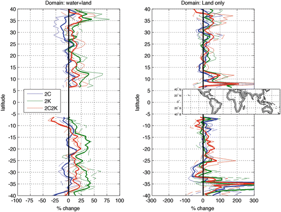
Changes in TC-related precipitation amount (TCPn) in the 2C (blue), 2K (green), and 2C2K (red) experiments as a function of latitude. Results are shown with respect to the CLIM experiment. Solid thin lines represent CMCC results. Dashed thin lines represent GFDL results. The solid thick lines represent the average of the two models. Units are [%]. Left panel refers to the entire TC track. Right panel refers to TC track over land only (the gray region represented in the small map)
-
2C: this is a doubling CO2 experiment. It is obtained by integrating the models with climatological SST (as in CLIM) but with a doubled concentration of atmospheric CO2 with respect to the CLIM experiment for 10 years.
-
2K: this experiment is obtained by integrating the models with climatological SST (as in CLIM) and adding a 2K globally uniform SST anomaly for 10 years.
-
2C2K: this experiment is made by combining the 2K and 2C perturbations.

A more detailed explanation of models and simulations can be found in Scoccimarro et al. (2014), Shaewitz et al. (2014), and Walsh et al. (2015).
The amount of rainfall associated with a TC, both in models and observations, is computed by considering the daily precipitation in a 10 × 10° box around the center of the storm (extending 5° from the center of the TC to the north, south, east, and west). According to previous studies (e.g., Lonfat et al. 2004; Larson et al. 2005; Kunkel et al. 2010), a 10 × 10° window is sufficient to include the majority of TC-related precipitation in most of the cases.
3 Results
The control simulation (CLIM) performed with the two models represent reasonably well the TC count at the global scale for the present climate, with a 9 % underestimation for the CMCC model and a 16 % overestimation for the GFDL model, compared to the reference value of 93.3 TCs/year obtained from the observation for the period 1997–2006. The CMCC model also tends to significantly underestimate the TC count in the Atlantic basin and Eastern Pacific (Fig. 10.1) as found by similar analyses using the coupled version of the ECHAM5 atmospheric model (Scoccimarro et al. 2011). A difficulty in representing TC activity in the Atlantic Basin is common to many climate models, as discussed in Lim et al. (2014).
In this work, we aim to assess the models’ ability in simulating precipitation associated with TCs and quantifying their relative changes for the three different idealized global forcing scenarios. To examine the TCP contribution to total precipitation, we accumulated TCP over the 10-year period, representing the present climate, and we compared it to the total precipitation for the same period. Figure 10.2 shows the composite of rainfall during the top 10 % rainiest TCs for the observations (left panel) and models (middle and right panels). TC rainfall patterns are reasonably well represented by models, as described by Villarini et al. (2014).

Composite mean observed (GPCP, left panel) and modeled (CMCC/GFDL central/right panels) daily rainfall rate patterns associated to the 10 % most intense TCs. The units are mm/day and the x and y axes correspond to degrees from the TC center
In the observations the TC rainfall represents a large contribution to the total rainfall over the Northwest Pacific, the Northeast Pacific, and the northwestern part of the Australian Basin (Fig. 10.3, upper panel). Over these regions, the amount of precipitation contribution due to TCs is as large as 40 %, reaching a maximum of 50 % in the Northwest Pacific. These features are captured by the simulations, despite the tendency of the CMCC model to underestimate the TCP fraction (Fig. 10.3 central panel). Both CMCC and GFDL models are able to represent the basic aspects of the latitudinal distribution of TCP, with the GFDL model showing a better agreement with the observations (Fig. 10.3 lower panel). In terms of absolute values, the modeled TCP zonal average, normalized by TC days (hereafter TCPn), shows maximum values at about 15° in both hemispheres (not shown).

Percentage of precipitation associated with TCs in the control simulation CLIM with respect to the total annual precipitation. The accumulation is performed by taking a 10 × 10° window centered on the center of circulation. The upper panel refers to the observations, while the central and lower panels to the CMCC and GFDL models, respectively. Units are [%]
Changes in TCPn are very similar for the two models and show a global increase in the 2K and 2C2K experiments but not for the 2C one (Fig. 10.4). The meridional distribution of TCPn changes (Fig. 10.4 left panel) in the 2C case shows the less pronounced changes within the three synthetic scenarios, with negative values over most of the latitudes, especially in the Northern Hemisphere. On the other hand, the 2K and 2C2K experiments show positive changes up to 45 % when considering the average of the two models (Fig. 10.4, red and green bold lines). The positive increase is more pronounced in the 2K experiment if compared to the 2C2K one. These results are consistent with Villarini et al. (2014) who found a widespread decrease in rainfall for the most intense TCs for the 2C experiment and a general increase in rainfall when SST was increased by 2K. This statement holds regardless of the distance from the center of circulation and for all the ocean basins.

TC genesis points in CMCC (central panel) and GFDL (lower panel) models, compared to the observations (upper panel) over the period 1981–1990
Focusing on the coastal region (shaded gray area in small map shown in Fig. 10.4), the TCPn increase in 2K and 2C2K is even more pronounced (Fig. 10.4, right panels), up to 200 %. In these areas even the 2C experiment shows positive changes in most latitudes. The resulting changes are spread out almost evenly over the coastal domain prone to TC landfall (not shown).
4 Discussion and Conclusion
It is well known that atmospheric moisture content tends to increase at a rate roughly governed by the Clausius–Clapeyron equation, while the energy available to drive convection increases more slowly (e.g., Knutson and Manabe 1995; Allen and Ingram 2002; Held and Soden 2006; Meehl et al. 2007). Therefore, in a warmer climate, we expect an increase in the water amount associated with phenomena leading to intense precipitation (such as TCs) larger than what it is expected in moderate events (Scoccimarro et al. 2013).
Our results show that the TC-associated precipitation is increased in the experiments with a 2K-SST increase. On the other hand, in the simulation with doubling of atmospheric CO2, the changes in TC rainfall are small and we found that, on average, the simulated TC rainfall tends to decrease compared to the present-day climate (Fig. 10.4). Since environmental humidity was found to correlate with a larger hurricane rain field (Matyas 2010), and because we should expect a strong relationship between changes in available precipitable water and changes in TC precipitation, we investigated changes in the vertically integrated atmospheric water vapor content under the different idealized warming scenarios. All the considered experiments show an increase in the water content over the tropical belt. The water content percentage increase (not shown here, see Scoccimarro et al. (2014), their Fig. 8) is about 1 % in 2C, 18 % in 2K, and 19 % in 2C2K, suggesting that the 1 % increment between 2K and 2C2K is mainly due to the higher atmospheric capability to hold moisture induced by the doubling of CO2, as shown in the 2C experiment. According to the Clausius–Clapeyron relationship, the lower-tropospheric temperature change found in the different experiments (about 0.1 K in the 2C, 2.2 K in the 2K, and 2.4 K in the 2C2K) should lead to a water content increase of about 1 %, 18 %, and 19 %, respectively, which is fully consistent with that obtained from the models.
Despite the increase in water content in all of the three warming experiments, the doubling of CO2 tends to reduce TCP, whereas the increase of 2K in SST tends to increase TCP. The reason should be found in the water balance at the surface: in 2K and 2C2K experiments (2Ks), we found a strong increase of the evaporation rate over the tropics (Fig. 10.5, left panel, green and red lines, respectively) due to the increase in saturated water vapor pressure at the surface. The 2K increase in SST leads to a net increase of the evaporation rate (E). This can be easily explained considering that E is proportional to the difference between saturated water vapor at the surface (es) and water vapor pressure of the lower tropospheric layers (ea) and that es depends on surface temperature following an exponential law, whereas ea follows the same law, scaled by a factor (less than 1) represented by the relative humidity. Therefore, an increase in temperature has different impacts on es and ea. The doubling of CO2, on the other hand, tends to reduce E (Fig. 10.5, blue line) independently of the boundary conditions. The doubling of CO2 in forced experiments (prescribed SST) induces a weakening effect on E, since the increase in the lower tropospheric temperature leads to an increase in ea, associated with no changes in es due to the fixed temperature forcing at the surface. This effect results in an increase of the atmospheric static stability in the 2C experiment.

Changes in evaporation (left panel) and precipitation (right panel) in 2C (blue), 2K (green) and 2C2K (red) experiments as a function of latitude with respect to the CLIM experiment. Solid thin lines represent CMCC results. Dashed thin lines represent GFDL results. Solid thick lines represent averaged values. Northern Hemisphere values are computed over June–November and Southern Hemisphere values are computed over December–May. Units are [%]
The CO2 doubling tends to slow down the global hydrological cycle by about 2 % (see Table 2 in Scoccimarro et al. 2014). This is also evident in the meridional distribution of evaporation and precipitation changes (blue lines in Fig. 10.5 left and right panels, respectively) during the TC season. The 2K SST increase induces an acceleration of the hydrological cycle of the order of 6–7 % that is reduced to 4–5 % if associated with the CO2 doubling (Fig. 10.5). The changes found in the hydrological cycle are strongly influenced by the TC precipitation: a 4 %/6 % (2C2K/2K) increase in the average precipitation corresponds to an increase of about 20 %/30 % in TC-related precipitation.
In summary, bearing in mind the limitation of the considered models in representing tropical convection (Lim et al. 2014), and the difficulty to provide a measure of reliability due to the low number of models involved (just two), the precipitation associated with TCs results in an increase in the experiments with a 2K-SST increase and to a decrease when atmospheric CO2 is doubled. This is consistent with the water balance at the surface, as a 2K increase in SST leads to a net increase of the evaporation rate, while doubling the atmospheric CO2 has the opposite effect.
Unexpectedly, between 7 and 12° in the Southern Hemisphere, the 2C2K experiment shows a reduction of the TC-associated precipitation. This feature will be the object of future work.
As already mentioned, the TCPn increase projected in all of the considered 2K-SST warming scenarios is more pronounced over land than what is expected considering also the TC path over the ocean (Fig. 10.4). It is well known that in some cases, during landfall, the TC precipitation tends to increase (Dong et al. 2010). This is mainly due to the lifting effect induced by orographic features (Huang et al. 2013). In our 2K-SST warming experiment, the more pronounced increase of the precipitation over land might be related to an additional lifting effect on the TC-associated air masses, when landfall occurs. Keeping in mind the possibility of an induced lifting effect source, we examined how humidity of the air is projected to change in the considered 2K-SST experiments. The specific humidity over the coastal regions (Fig. 10.6) in the CLIM experiment is very similar to what is found over the entire domain including its ocean portion, with differences of the order of mg/Kg (not shown). In the 2C experiment, no significant differences are found in the specific humidity over land (Fig. 10.7, upper panel). On the other hand, the two experiments implying 2K-SST warming show substantial changes in the meridional distribution of the specific humidity: in the first levels of the atmospheric column (between the surface and 300 hPa), there are positive changes, over most of the tropical latitudes (Fig. 10.7 central and lower panels): the specific humidity increase is up to 20 % of the CLIM value. The more pronounced increase in TCPn over land in 2K-SST experiments is consistent with such specific humidity increase in the lower levels of the atmospheric column: TCs at landfall are projected to encounter a less stable atmospheric column, since the air at the lower levels is wetter in this experiment due to increased SSTs. A more unstable atmospheric column, induced by the availability of more moist air at low levels, leads to increased updrafts, thus to an increased condensation into droplets.

Meridional distribution of the specific humidity in CLIM experiment during the TC season (June–November for the Northern Hemisphere and December–May for the Southern Hemisphere) considering coastal region only. Ensemble averages are shown. Units are [g/kg]

Meridional distribution of the specific humidity changes during the TC season (June–November for the Northern Hemisphere and December–May for the Southern Hemisphere). Figure shows specific humidity changes in the three different scenarios (2C/2K/2C2K in upper-right/central-right/lover-right panels), compared to the CLIM experiment. Only land regions are considered. Ensemble averages are shown. Units are [g/kg]
References
Allen MR, Ingram WJ (2002) Constraints on future changes in climate and the hydrologic cycle. Nature 419:224–232. doi:10.1038/nature01092
Bolvin DT, Adler RF, Huffman GJ et al (2009) Comparison of GPCP monthly and daily precipitation estimates with high-latitude gauge observations. J Appl Meteorol Climatol 48:1843–1857. doi:10.1175/2009JAMC2147.1
Dong M, Chen L, Li Y, Lu C (2010) Rainfall reinforcement associated with landfalling tropical cyclones. J Atmos Sci 67:3541–3558. doi:10.1175/2010JAS3268.1
Held IM, Soden BJ (2006) Robust responses of the hydrological cycle to global warming. J Climate 19:5686–5699. doi:10.1175/JCLI3990.1
Horn M, Walsh K, Zhao M et al (2014) Tracking scheme dependence of simulated tropical cyclone response to idealized climate simulations. J Climate 27:9197–9213. doi:10.1175/JCLI-D-14-00200.1
Huang H-L, Yang M-J, Sui C-H (2013) Water budget and precipitation efficiency of typhoon Morakot (2009). J Atmos Sci 71:112–129. doi:10.1175/JAS-D-13-053.1
Huffman GJ, Adler RF, Morrissey MM et al (2001) Global precipitation at one-degree daily resolution from multisatellite observations. J Hydrometeorol 2:36–50. doi:10.1175/1525-7541(2001)002<0036:GPAODD>2.0.CO;2
JTWC (2013) Annual tropical cyclone report. Joint Typhoon Warning Center, Pearl Harbor
Knutson TR, Manabe S (1995) Time-mean response over the tropical pacific to increased C02 in a coupled Ocean-Atmosphere Model. J Climate 8:2181–2199. doi:10.1175/1520-0442(1995)008<2181:TMROTT>2.0.CO;2
Knutson TR, McBride JL, Chan J et al (2010) Tropical cyclones and climate change. Nat Geosci 3:157–163. doi:10.1038/ngeo779
Knutson TR, Sirutis JJ, Vecchi GA et al (2013) Dynamical downscaling projections of twenty-first-century Atlantic hurricane activity: CMIP3 and CMIP5 model-based scenarios. J Climate 26:6591–6617. doi:10.1175/JCLI-D-12-00539.1
Kunkel KE, Easterling DR, Kristovich DAR et al (2010) Recent increases in U.S. heavy precipitation associated with tropical cyclones. Geophys Res Lett. doi:10.1029/2010GL045164
Landsea CW, Franklin JL (2013) Atlantic hurricane database uncertainty and presentation of a new database format. Mon Weather Rev 141:3576–3592. doi:10.1175/MWR-D-12-00254.1
Larson J, Zhou Y, Higgins RW (2005) Characteristics of landfalling tropical cyclones in the United States and Mexico: climatology and interannual variability. J Climate 18:1247–1262. doi:10.1175/JCLI3317.1
Lim Y-K, Schubert SD, Reale O et al (2014) Sensitivity of tropical cyclones to parameterized convection in the NASA GEOS-5 model. J Climate 28:551–573. doi:10.1175/JCLI-D-14-00104.1
Lonfat M, Marks FD, Chen SS (2004) Precipitation distribution in tropical cyclones using the Tropical Rainfall Measuring Mission (TRMM) microwave imager: a global perspective. Mon Weather Rev 132:1645–1660. doi:10.1175/1520-0493(2004)132<1645:PDITCU>2.0.CO;2
Matyas CJ (2010) Associations between the size of hurricane rain fields at landfall and their surrounding environments. Meteorol Atmos Phys 106:135–148. doi:10.1007/s00703-009-0056-1
Meehl GA, Stocker TF, Collins WD et al (2007) Global climate projections. In: Solomon S, Qin D, Manning M et al (eds) Climate change 2007: the physical science basis. Cambridge University Press, Cambridge, UK, pp 748–845
Mendelsohn R, Emanuel K, Chonabayashi S, Bakkensen L (2012) The impact of climate change on global tropical cyclone damage. Nat Clim Chang 2:205–209. doi:10.1038/nclimate1357
Pielke RA Jr, Gratz J, Landsea CW et al (2008) Normalized hurricane damage in the United States: 1900–2005. Nat Hazards Rev 9:29–42. doi:10.1061/(ASCE)1527-6988(2008)9:1(29)
Rappaport EN (2000) Loss of life in the United States associated with recent Atlantic Tropical Cyclones. Bull Am Meteorol Soc 81:2065–2073. doi:10.1175/1520-0477(2000)081<2065:LOLITU>2.3.CO;2
Roeckner E, Bäuml G, Bonaventura L et al (2003) The atmospheric general circulation model ECHAMM5. Part 1: model description. Max-Planck-Institut für Meteorologie, Hamburg
Scoccimarro E, Gualdi S, Bellucci A et al (2011) Effects of tropical cyclones on ocean heat transport in a high-resolution coupled general circulation model. J Climate 24:4368–4384. doi:10.1175/2011JCLI4104.1
Scoccimarro E, Gualdi S, Bellucci A et al (2013) Heavy precipitation events in a warmer climate: results from CMIP5 models. J Climate 26:7902–7911. doi:10.1175/JCLI-D-12-00850.1
Scoccimarro E, Gualdi S, Villarini G et al (2014) Intense precipitation events associated with landfalling tropical cyclones in response to a warmer climate and increased CO2. J Climate 27:4642–4654. doi:10.1175/JCLI-D-14-00065.1
Shaevitz DA, Camargo SJ, Sobel AH et al (2014) Characteristics of tropical cyclones in high-resolution models in the present climate. J Adv Model Earth Syst 6:1154–1172. doi:10.1002/2014MS000372
Villarini G, Lavers DA, Scoccimarro E et al (2014) Sensitivity of tropical cyclone rainfall to idealized global-scale forcings. J Climate 27:4622–4641. doi:10.1175/JCLI-D-13-00780.1
Walsh K, Lavender S, Scoccimarro E, Murakami H (2013) Resolution dependence of tropical cyclone formation in CMIP3 and finer resolution models. Clim Dyn 40:585–599. doi:10.1007/s00382-012-1298-z
Walsh KJE, Camargo SJ, Vecchi GA et al (2015) Hurricanes and climate: the U.S. CLIVAR Working Group on hurricanes. Bull Am Meteorol Soc 96:997–1017. doi:10.1175/BAMS-D-13-00242.1
Zhao M, Held IM, Lin S-J, Vecchi GA (2009) Simulations of global hurricane climatology, interannual variability, and response to global warming using a 50-km resolution GCM. J Climate 22:6653–6678. doi:10.1175/2009JCLI3049.1
Acknowledgment
This work was carried out as part of a Hurricane and Climate Working Group activity supported by the US CLIVAR. We acknowledge the support provided by Naomi Henderson, who downloaded and organized the data at the Lamont data library. The research leading to these results has received funding from the Italian Ministry of Education, University and Research and the Italian Ministry of Environment, Land and Sea under the GEMINA project (Enrico Scoccimarro). Moreover this material is based in part upon work supported by the National Science Foundation under Grant No. AGS-1262099 (Gabriele Villarini). The authors also acknowledge the support of their respective institutions and the precious comments received by the reviewers.
Author information
Authors and Affiliations
Corresponding author
Editor information
Editors and Affiliations
Rights and permissions
Copyright information
© 2017 Springer International Publishing AG
About this chapter
Cite this chapter
Scoccimarro, E. et al. (2017). Tropical Cyclone Rainfall Changes in a Warmer Climate. In: Collins, J., Walsh, K. (eds) Hurricanes and Climate Change. Springer, Cham. https://doi.org/10.1007/978-3-319-47594-3_10
Download citation
DOI: https://doi.org/10.1007/978-3-319-47594-3_10
Published:
Publisher Name: Springer, Cham
Print ISBN: 978-3-319-47592-9
Online ISBN: 978-3-319-47594-3
eBook Packages: Earth and Environmental ScienceEarth and Environmental Science (R0)