Carrier Phase Integer Ambiguity Resolution

Zusammenfassung

Global Navigation Satellite System (GlossaryTerm

GNSS

) carrier-phase integer ambiguity resolution is the process of resolving the carrier-phase ambiguities as integers. It is the key to fast and high-precision GNSS parameter estimation and it applies to a great variety of GNSS models that are currently in use in navigation, surveying, geodesy and geophysics. The theory that underpins GNSS carrier-phase ambiguity resolution is the theory of integer inference. This theory and its practical application is the topic of the present chapter.

Carrier-phase integer ambiguity resolution is the key to fast and high-precision GNSS parameter estimation. It is the process of resolving the unknown cycle ambiguities of the carrier-phase data as integers. Once this has been done successfully, the very precise carrier-phase data will act as very precise pseudorange data, thus making very precise positioning and navigation possible.

GNSS ambiguity resolution applies to a great variety of current and future GNSS models, with applications in surveying, navigation, geodesy and geophysics. These models may differ greatly in complexity and diversity. They range from single-receiver or single-baseline models used for kinematic positioning to multibaseline models used as a tool for studying geodynamic phenomena. The models may or may not have the relative receiver-satellite geometry included. They may also be discriminated as to whether the slave receiver(s) is stationary or in motion, or whether or not the differential atmospheric delays (ionosphere and troposphere) are included as unknowns. An overview of these models can be found in textbooks like [23.1, 23.2, 23.3, 23.4, 23.5] and in the Chaps. 21, 25, and 26 of this Handbook.

The theory that underpins ultraprecise GNSS carrier-phase ambiguity resolution is the theory of integer inference [23.6, 23.7]. This theory of integer estimation and validation is the topic of the present chapter. Although the theory was originally developed for Global Positioning System (GlossaryTerm

GPS

) [23.10, 23.11, 23.12, 23.13, 23.14, 23.8, 23.9], the theory has a much wider range of applicability. Next to the regional and global satellite navigation systems, it also applies to other carrier-phase-based interferometric techniques, such as Very Long Baseline Interferometry (GlossaryTerm

VLBI

) [23.15], Interferometric Synthetic Aperture Radar (GlossaryTerm

InSAR

) [23.16], or underwater acoustic carrier-phase positioning [23.17].

This chapter is organized as follows. In Sect. 23.1, the mixed-integer GNSS model is introduced. It forms the basis of all integer ambiguity resolution methods. An overview of the various ambiguity resolution steps is given, together with an evaluation of their contribution to the overall quality.

In Sect. 23.2, the ambiguity resolution methods of integer rounding (GlossaryTerm

IR

) and integer bootstrapping (GlossaryTerm

IB

) are presented, together with practical expressions for evaluating their ambiguity success rates. These methods are the simplest methods available, but their performance depends on the chosen ambiguity parametrization.

In Sect. 23.3 it is shown how the performance of rounding and bootstrapping can be improved by using certain ambiguity parametrizations. This includes a description of the decorrelating Z-transformation by which these improvements can be realized. Various examples that illustrate the concepts involved are also given.

The method of integer least-squares (GlossaryTerm

ILS

s) ambiguity resolution is described in Sect. 23.4. This method is optimal in the sense that it achieves the highest success rate of all ambiguity resolution methods. The method is however also more complex as it requires an integer search over an ambiguity search space. It is shown how to make the method numerically efficient by combining the integer search with ambiguity decorrelation. Methods for computing or bounding the ILS success rate are also given.

The concept of partial ambiguity resolution is presented in Sect. 23.5 . It is an alternative to full ambiguity resolution in case the resolution of all ambiguities cannot be done with a sufficiently high success rate.

As wrongly fixed integer ambiguities can result in unacceptably large positioning errors, it is important to have rigorous testing methods in place for accepting or rejecting the computed integer ambiguity solution. These methods and their theoretical foundation are presented in Sect. 23.6.

1 GNSS Ambiguity Resolution

1.1 The GNSS Model

To formulate the GNSS model for ambiguity resolution, we start with the observation equations for the pseudorange (code) and carrier-phase observables. If we denote the j-frequency pseudorange and carrier-phase for the r-s receiver–satellite combination at epoch t as $p_{r,j}^{s}(t)$ and $\phi_{r,j}^{s}(t)$ respectively, then their observation equations can be formulated as [23.1, 23.2, 23.3, 23.4, 23.5],

$$\begin{aligned}p_{r,j}^{s}(t)&=\rho_{r}^{s}(t)+T_{r}^{s}(t)+I_{r,j}^{s}(t)\\ &\quad\,+cdt_{r,j}^{s}(t)+e_{r,j}^{s}(t)\;,\\ \varphi_{r,j}^{s}(t)&=\rho_{r}^{s}(t)+T_{r}^{s}(t)-I_{r,j}^{s}(t)\\ &\quad\,+c\delta t_{r,j}^{s}(t)+\lambda_{j}N_{r,j}^{s}+\epsilon_{r,j}^{s}(t)\;,\end{aligned}$$

(23.1)

where $\rho_{r}^{s}$ is the receiver–satellite range, $T_{r}^{s}(t)$ and $I_{r}^{s}$ are the tropospheric and ionospheric path delays, $dt_{r,j}^{s}$ and $\delta t_{r,j}^{s}$ are the pseudorange and carrier-phase receiver–satellite clock biases, $N_{r,j}^{s}$ is the time-invariant integer carrier-phase ambiguity, c is the speed of light, λ _j is the j-frequency wavelength, and $e_{r,j}^{s}$, $\epsilon_{r,j}^{s}$ are the remaining error terms respectively.

The receiver–satellite range $\rho_{r}^{s}$ in (23.1) is usually further linearized in the receiver- or satellite-position coordinates. As a result one obtains linear equations that can be used to form a system of linear equations for solving the unknown parameters of position, atmosphere, clock and ambiguities. Hence, if we assume the error terms $e_{r,j}^{s}$ and $\epsilon_{r,j}^{s}$ in (23.1) to be zero-mean random variables, the linear(ized) system of observation equations can be used to set up a linear model in which some of the unknown parameters are reals and others are integer. Such a GNSS model is an example of a mixed-integer linear model.

We now define the general form of the mixed-integer GNSS model .

Definition 23.1 Mixed-integer GNSS model

Let $(\mathbf{A},\mathbf{B})$ be a given $m\times(n+p)$ matrix of full rank and let $\mathbf{Q}_{\boldsymbol{y}\boldsymbol{y}}$ be a given m × m positive definite matrix. Then

$$\boldsymbol{y}\sim\mathrm{N}(\mathbf{A}\boldsymbol{a}+\mathbf{B}\boldsymbol{b},\mathbf{Q}_{\boldsymbol{y}\boldsymbol{y}})\;,\;\boldsymbol{a}\in\mathbb{Z}^{n}\;,\;\boldsymbol{b}\in\mathbb{R}^{p}$$

(23.2)

will be referred to as the mixed-integer GNSS model.

The notation ∼ is used to describe distributed as. The m-vector y contains the pseudorange and carrier-phase observables, the n-vector a the integer ambiguities, and the real-valued p-vector b the remaining unknown parameters, such as, for example, position coordinates, atmospheric delay parameters (troposphere, ionosphere) and clock parameters. As in most GNSS applications, the underlying probability distribution of the data is assumed to be a multivariate normal distribution.

1.2 Ambiguity Resolution Steps

The purpose of ambiguity resolution is to exploit the integer constraints, $\boldsymbol{a}\in\mathbb{Z}^{n}$ in (23.2), so as to get a better estimator of b than otherwise would be the case. The mixed-integer GNSS model (23.2) can be solved in the following steps:

• 1. Float Solution : In the first step, the integer nature of the ambiguities is discarded and a standard least-squares (LS) parameter estimation is performed. As a result, one obtains the so-called float solution, together with its variance-covariance matrix,

  $$\begin{bmatrix}\hat{\boldsymbol{a}}\\ \hat{\boldsymbol{b}}\end{bmatrix}\;\sim\;\mathrm{N}\left(\begin{bmatrix}\boldsymbol{a}\\ \boldsymbol{b}\end{bmatrix},\begin{bmatrix}\mathbf{Q}_{\hat{\boldsymbol{a}}\hat{\boldsymbol{a}}}&\mathbf{Q}_{\hat{\boldsymbol{a}}\hat{\boldsymbol{b}}}\\ \mathbf{Q}_{\hat{\boldsymbol{b}}\hat{\boldsymbol{a}}}&\mathbf{Q}_{\hat{\boldsymbol{b}}\hat{\boldsymbol{b}}}\end{bmatrix}\right).$$

  (23.3)

  Other forms than batch least-squares – such as recursive LS or Kalman filtering – may also be used to come up with a float solution. Such choices will depend on the application and on the structure of the GNSS model.

• 2. Integer Solution: The purpose of this second step is to take the integer constraints $\boldsymbol{a}\in\mathbb{Z}^{n}$ (23.2 ) into account. Hence, a mapping $\mathcal{I}:\mathbb{R}^{n}\mapsto\mathbb{Z}^{n}$ is introduced that maps the float ambiguities to corresponding integer values,

  $$\check{\boldsymbol{a}}=\mathcal{I}(\hat{\boldsymbol{a}})\;.$$

  (23.4)

  Many such integer mappings $\mathcal{I}$ exist. Popular choices are integer rounding (IR), integer bootstrapping (IB) and integer least-squares (ILS), see Sects. 23.2 and 23.4.

• 3. Fixed Solution : In the final step, once $\check{\boldsymbol{a}}$ is accepted, the ambiguity residual $\hat{\boldsymbol{a}}-\check{\boldsymbol{a}}$ is used to readjust the float estimator $\hat{\boldsymbol{b}}$ to obtain the so-called fixed estimator

  $$\check{\boldsymbol{b}}=\hat{\boldsymbol{b}}-\mathbf{Q}_{\hat{\boldsymbol{b}}\hat{\boldsymbol{a}}}\mathbf{Q}_{\hat{\boldsymbol{a}}\hat{\boldsymbol{a}}}^{-1}(\hat{\boldsymbol{a}}-\check{\boldsymbol{a}})\;.$$

  (23.5)

The fixed solution has a quality that is commensurate with the high precision of the phase data, provided the probability of $\check{\boldsymbol{a}}$ being the correct integer is sufficiently high. Figure 23.1 illustrates the high gain in positioning precision that can be achieved with successful ambiguity resolution.

Fig. 23.1a,b

Three-dimensional scatterplot of GPS position errors for short-baseline, dual-frequency instantaneous ambiguity float solutions ((a); $\hat{b}$) and corresponding ambiguity fixed position solutions ((b); $\check{b}$) (after [23.18]). Note the two orders of magnitude difference in scale between the two panels. dE, dN, and dU denote the components of the position errors in north, east and up direction

1.3 Ambiguity Resolution Quality

To determine the quality of the fixed solution $\check{\boldsymbol{b}}$ (23.5), we need to propagate the probabilistic properties of its constituents:

• 1. Quality of float solution: The float solution is defined as the minimizer of the unconstrained LS-problem,

  $$(\hat{\boldsymbol{a}},\hat{\boldsymbol{b}})=\arg\min_{\boldsymbol{a}\in\mathbb{R}^{n},\boldsymbol{b}\in\mathbb{R}^{p}}\|\boldsymbol{y}-\mathbf{A}\boldsymbol{a}-\mathbf{B}\boldsymbol{b}\|^{2}_{\mathbf{Q}_{\boldsymbol{y}\boldsymbol{y}}}$$

  (23.6)

  the solution of which follows from solving the normal equations

  $$\begin{bmatrix}\mathbf{A}^{\top}\mathbf{Q}_{\boldsymbol{y}\boldsymbol{y}}^{-1}\mathbf{A}&\mathbf{A}^{\top}\mathbf{Q}_{\boldsymbol{y}\boldsymbol{y}}^{-1}\mathbf{B}\\ \mathbf{B}^{\top}\mathbf{Q}_{\boldsymbol{y}\boldsymbol{y}}^{-1}\mathbf{A}&\mathbf{B}^{\top}\mathbf{Q}_{\boldsymbol{y}\boldsymbol{y}}^{-1}\mathbf{B}\end{bmatrix}\begin{bmatrix}\hat{\boldsymbol{a}}\\ \hat{\boldsymbol{b}}\end{bmatrix}=\begin{bmatrix}\mathbf{A}^{\top}\mathbf{Q}_{\boldsymbol{y}\boldsymbol{y}}^{-1}\boldsymbol{y}\\ \mathbf{B}^{\top}\mathbf{Q}_{\boldsymbol{y}\boldsymbol{y}}^{-1}\boldsymbol{y}\end{bmatrix}.$$

  (23.7)

  This solution is given as

  $$\begin{aligned}\hat{\boldsymbol{a}}&=(\bar{\mathbf{A}}^{\top}\mathbf{Q}_{\boldsymbol{y}\boldsymbol{y}}^{-1}\bar{\mathbf{A}})^{-1}\bar{\mathbf{A}}^{\top}\mathbf{Q}_{\boldsymbol{y}\boldsymbol{y}}^{-1}\boldsymbol{y}\\ \hat{\boldsymbol{b}}&=(\mathbf{B}^{\top}\mathbf{Q}_{\boldsymbol{y}\boldsymbol{y}}^{-1}\mathbf{B})^{-1}\mathbf{B}^{\top}\mathbf{Q}_{\boldsymbol{y}\boldsymbol{y}}^{-1}(\boldsymbol{y}-\mathbf{A}\hat{\boldsymbol{a}})\;,\end{aligned}$$

  (23.8)

  where $\bar{\mathbf{A}}=\mathbf{P}_{\mathbf{B}}^{\perp}\mathbf{A}$, with orthogonal projector

  $$\mathbf{P}_{\mathbf{B}}^{\perp}=\mathbf{I}_{m}-\mathbf{B}(\mathbf{B}^{\top}\mathbf{Q}_{\boldsymbol{y}\boldsymbol{y}}^{-1}\mathbf{B})^{-1}\mathbf{B}^{\top}\mathbf{Q}_{\boldsymbol{y}\boldsymbol{y}}^{-1}\;.$$

  With the distributional assumptions of (23.2), the distribution of the ambiguity float solution follows as the multivariate normal distribution $\hat{\boldsymbol{a}}\sim\mathrm{N}(\boldsymbol{a},\mathbf{Q}_{\hat{\boldsymbol{a}}\hat{\boldsymbol{a}}})$, with variance matrix

  $$\mathbf{Q}_{\hat{\boldsymbol{a}}\hat{\boldsymbol{a}}}=(\bar{\mathbf{A}}^{\top}\mathbf{Q}_{\boldsymbol{y}\boldsymbol{y}}^{-1}\bar{\mathbf{A}})^{-1}\;.$$

  (23.9)

  The probability density function (GlossaryTerm

  PDF

  ) of $\hat{\boldsymbol{a}}$ is thus given as
  $$\begin{aligned}&f_{\hat{\boldsymbol{a}}}(\boldsymbol{x}|\boldsymbol{a})\\ &\quad=\frac{1}{\sqrt{\mathrm{det}(2\uppi\mathbf{Q}_{\hat{\boldsymbol{a}}\hat{\boldsymbol{a}}})}}\exp\left(-\frac{1}{2}||\boldsymbol{x}-\boldsymbol{a}||_{\mathbf{Q}_{\hat{\boldsymbol{a}}\hat{\boldsymbol{a}}}}^{2}\right).\end{aligned}$$

  (23.10)

  Its shape is completely determined by the ambiguity variance matrix $\mathbf{Q}_{\hat{\boldsymbol{a}}\hat{\boldsymbol{a}}}$, which in its turn is completely determined by the GNSS model’s design matrix, $(\mathbf{A},\mathbf{B})$, and observation variance matrix $\mathbf{Q}_{\boldsymbol{y}\boldsymbol{y}}$. The PDF of $\hat{\boldsymbol{a}}$ is needed to determine the probability mass function (GlossaryTerm

  PMF

  ) of $\check{\boldsymbol{a}}$ in step 2.

• 2. Quality of integer solution: Since the integer map of step 2, $\mathcal{I}:\mathbb{R}^{n}\mapsto\mathbb{Z}^{n}$, is a many-to-one map, different real-valued vectors will be mapped to one and the same integer vector. One can therefore assign a subset, say $\mathcal{P}_{\boldsymbol{z}}\subset\mathbb{R}^{n}$, to each integer vector $\boldsymbol{z}\in\mathbb{Z}^{n}$,

  $$\mathcal{P}_{\boldsymbol{z}}=\{\boldsymbol{x}\in\mathbb{R}^{n}\mid\boldsymbol{z}=\mathcal{I}(\boldsymbol{x})\},\;\;\;\boldsymbol{z}\in\mathbb{Z}^{n}\;.$$

  (23.11)

  This subset is referred to as the pull-in region of z. It is the region in which all vectors are pulled to the same integer vector z. The pull-in regions are translational invariant over the integers and cover the whole space $\mathbb{R}^{n}$ without gaps and overlap [23.19]. Two-dimensional examples of pull-in regions are shown in Fig. 23.2. They are the pull-in regions of integer rounding, integer bootstrapping and integer least-squares.

  Fig. 23.2a–c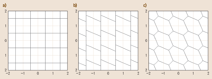

  

  Two-dimensional pull-in regions of integer rounding (a), integer bootstrapping (b), and integer least-squares (c)

  The PMF of $\check{\boldsymbol{a}}$ follows from integrating the PDF of $\hat{\boldsymbol{a}}$ over the pull-in regions. Since $\check{\boldsymbol{a}}=\boldsymbol{z}\in\mathbb{Z}^{n}$ iff $\hat{\boldsymbol{a}}\in\mathcal{P}_{\boldsymbol{z}}$, the PMF of $\check{\boldsymbol{a}}$ follows as

  $$P(\check{\boldsymbol{a}}=\boldsymbol{z})=P(\hat{\boldsymbol{a}}\in\mathcal{P}_{\boldsymbol{z}})=\int\limits_{\mathcal{P}_{\boldsymbol{z}}}f_{\hat{\boldsymbol{a}}}(\boldsymbol{x}|\boldsymbol{a})\mathrm{d}\boldsymbol{x}\;.$$

  (23.12)

  A two-dimensional example of an ambiguity PDF and corresponding PMF is given in Fig. 23.3a,b.

  Fig. 23.3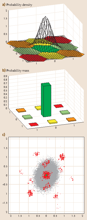

  

  (a) Gaussian probability density function (PDF) $f_{\hat{\boldsymbol{a}}}(\boldsymbol{x}|\boldsymbol{a})$ with (hexagon) ILS pull-in regions. (b) Corresponding probability mass function (PMF) $P(\check{\boldsymbol{a}}_{\mathrm{ILS}}=\boldsymbol{z})$ of ILS estimator. (c) Scatterplot of horizontal position errors for float solution (gray dots) and corresponding fixed solution (green and red dots). In this case, 93 % of the solutions were correctly fixed (green dots), and 7 % were wrongly fixed (red dots) (after [23.18])

  Of all the probabilities of the PMF, the probability of correct integer estimation, $P(\check{\boldsymbol{a}}=\boldsymbol{a})$, is of particular importance for ambiguity resolution. This probability is referred to as the ambiguity success rate and it is given by the integral

  $$\begin{aligned}P_{\text{s}}=P(\check{\boldsymbol{a}}=\boldsymbol{a})&=\int\limits_{\mathcal{P}_{\boldsymbol{a}}}f_{\hat{\boldsymbol{a}}}(\boldsymbol{x}|\boldsymbol{a})\mathrm{d}\boldsymbol{x}\\ &=\int\limits_{\mathcal{P}_{\boldsymbol{0}}}f_{\hat{\boldsymbol{a}}}(\boldsymbol{x}|\boldsymbol{0})\mathrm{d}\boldsymbol{x}\;,\end{aligned}$$

  (23.13)

  where the last line follows from the translational property $f_{\hat{\boldsymbol{a}}}(\boldsymbol{x}+\boldsymbol{a}|\boldsymbol{a})=f_{\hat{\boldsymbol{a}}}(\boldsymbol{x}|\boldsymbol{0})$ of the multivariate normal distribution.

  Note that the success rate P_s depends on the pull-in region $\mathcal{P}_{\boldsymbol{0}}$ and on the PDF $f_{\hat{\boldsymbol{a}}}(\boldsymbol{x}|\boldsymbol{0})$. Hence, the success rate is determined by the mapping $\mathcal{I}:\mathbb{R}^{n}\mapsto\mathbb{Z}^{n}$ and the ambiguity variance matrix $\mathbf{Q}_{\hat{\boldsymbol{a}}\hat{\boldsymbol{a}}}$, i. e., by the choice of integer estimator and the precision of the float ambiguities.

  Due to the shape of the pull-in regions and the nondiagonality of the ambiguity variance matrix, the computation of the ambiguity success rate is nontrivial. The evaluation of the multivariate integral (23.13) can generally be done through Monte Carlo integration [23.20], see also Sect. 23.4.3. For some important integer estimators we also have easy-to-compute expressions and/or sharp (lower and upper) bounds of their success rates available (Sect. 23.2).

• 3. Quality of fixed solution: Once the integer solution is available, the fixed solution is computed as in (23.5 ). This fixed solution has the multimodal PDF [23.21]

  $$f_{\check{\boldsymbol{b}}}(\boldsymbol{x})=\sum_{\boldsymbol{z}\in\mathbb{Z}^{n}}f_{\hat{\boldsymbol{b}}(\boldsymbol{z})}(\boldsymbol{x})P(\check{\boldsymbol{a}}=\boldsymbol{z})$$

  (23.14)

  in which $f_{\hat{\boldsymbol{b}}(\boldsymbol{z})}(\boldsymbol{x})$ denotes the PDF of the conditional LS-estimator

  $$\hat{\boldsymbol{b}}(\boldsymbol{z})=\hat{\boldsymbol{b}}-\mathbf{Q}_{\hat{\boldsymbol{b}}\hat{\boldsymbol{a}}}\mathbf{Q}_{\hat{\boldsymbol{a}}\hat{\boldsymbol{a}}}^{-1}(\hat{\boldsymbol{a}}-\boldsymbol{z}),$$

  normally distributed with mean and variance matrix,

  $$\begin{aligned}\boldsymbol{b}(\boldsymbol{z})&=\boldsymbol{b}-\mathbf{Q}_{\hat{\boldsymbol{b}}\hat{\boldsymbol{a}}}\mathbf{Q}_{\hat{\boldsymbol{a}}\hat{\boldsymbol{a}}}^{-1}(\boldsymbol{a}-\boldsymbol{z})\;,\\ \mathbf{Q}_{\hat{\boldsymbol{b}}(\boldsymbol{z})\hat{\boldsymbol{b}}(\boldsymbol{z})}&=\mathbf{Q}_{\hat{\boldsymbol{b}}\hat{\boldsymbol{b}}}-\mathbf{Q}_{\hat{\boldsymbol{b}}\hat{\boldsymbol{a}}}\mathbf{Q}_{\hat{\boldsymbol{a}}\hat{\boldsymbol{a}}}^{-1}\mathbf{Q}_{\hat{\boldsymbol{a}}\hat{\boldsymbol{b}}}\;.\end{aligned}$$

  (23.15)

  From (23.14) it follows that

  $$f_{\check{\boldsymbol{b}}}(\boldsymbol{x})\approx f_{\hat{\boldsymbol{b}}(\boldsymbol{a})}(\boldsymbol{x})\sim\mathrm{N}(\boldsymbol{b},\mathbf{Q}_{\hat{\boldsymbol{b}}(\boldsymbol{z})\hat{\boldsymbol{b}}(\boldsymbol{z})})$$

  (23.16)

  if

  $$P_{\text{s}}=P(\check{\boldsymbol{a}}=\boldsymbol{a})\approx 1\;.$$

  (23.17)

  Thus if the success rate is sufficiently close to one, the distribution of the fixed solution $\check{\boldsymbol{b}}$ can be approximated by the unimodal normal distribution $\mathrm{N}(\boldsymbol{b},\mathbf{Q}_{\hat{\boldsymbol{b}}(\boldsymbol{z})\hat{\boldsymbol{b}}(\boldsymbol{z})})$ of which the precision is better than that of the float solution $\hat{\boldsymbol{b}}$, $\mathbf{Q}_{\hat{\boldsymbol{b}}(\boldsymbol{z})\hat{\boldsymbol{b}}(\boldsymbol{z})}<\mathbf{Q}_{\hat{\boldsymbol{b}}\hat{\boldsymbol{b}}}$.

The relevance of ambiguity resolution and the need to have sufficiently large success rates is illustrated in Fig. 23.3c. It shows scatterplots of float positions (gray scatter) and corresponding fixed positions (green/red scatter). The small size of the green scatter shows the improvements that can be achieved over the float solution if the ambiguities are correctly fixed. The large red scatter indicates however that in this case the success rate is not large enough ($P_{\text{s}}={\mathrm{93}}\%$) to avoid some of the fixed positions being even poorer than the float positions. This underlines the importance of working with sufficiently high success rates only.

2 Rounding and Bootstrapping

2.1 Integer Rounding

The simplest integer estimator is rounding to the nearest integer. In the scalar case, its pull-in regions (intervals) are given as

$$\mathcal{R}_{z}=\left\{x\in\mathbb{R}\;\left|\vphantom{\sum}\right.\;|x-z|\leq\frac{1}{2}\right\},\;z\in\mathbb{Z}\;.$$

(23.18)

Any outcome of $\hat{a}\sim\mathrm{N}(a\in\mathbb{Z},\sigma_{\hat{a}}^{2})$, that satisfies $|\hat{a}-z|\leq 1/2$, will thus be pulled to the integer z. We denote the rounding estimator as $\check{a}_{\mathrm{R}}$ and the operation of integer rounding as $\lceil.\rfloor$. Thus $\check{a}_{\mathrm{R}}=\lceil\hat{a}\rfloor$ and $\check{a}_{\mathrm{R}}=z$ if $\hat{a}\in\mathcal{R}_{z}$.

The PMF of $\check{a}_{\mathrm{R}}=\lceil\hat{a}\rfloor$ is given as

$$\begin{aligned}&P(\check{a}_{\mathrm{R}}=z)\\ &\quad=\left[\Phi\left(\frac{1-2(a-z)}{2\sigma_{\hat{a}}}\right)+\Phi\left(\frac{1+2(a-z)}{2\sigma_{\hat{a}}}\right)-1\right],\\ &\qquad z\in\mathbb{Z}\;,\end{aligned}$$

(23.19)

where $\Phi(x)$ denotes the normal distribution function,

$$\Phi(x)=\int_{-\infty}^{x}\frac{1}{\sqrt{2\uppi}}\exp\left(-\frac{1}{2}v^{2}\right)\mathrm{d}v\;.$$

The PMF becomes more peaked when $\sigma_{\hat{a}}$ gets smaller. The success rate of scalar rounding follows from (23.19) by setting z equal to a,

$$P(\check{a}_{\mathrm{R}}=a)=2\Phi\left(\frac{1}{2\sigma_{\hat{a}}}\right)-1\;.$$

(23.20)

The behavior of the success rate as function of the ambiguity standard deviation $\sigma_{\hat{a}}$ is shown in Fig. 23.4. It shows that a success rate better than 99 %, requires $\sigma_{\hat{a}}<0.20$ cycle.

Fig. 23.4

Scalar rounding success rate versus ambiguity standard deviation σ in cycles

2.2 Vectorial Rounding

Scalar rounding is easily generalized to the vectorial case. It is defined as the componentwise rounding of $\hat{\boldsymbol{a}}=(\hat{a}_{1},\ldots,\hat{a}_{n})^{\top}$, $\check{\boldsymbol{a}}_{\mathrm{R}}=(\left\lceil\hat{a}_{1}\right\rfloor,\left\lceil\hat{a}_{2}\right\rfloor,\ldots,\left\lceil\hat{a}_{n}\right\rfloor)^{\top}$. The pull-in regions of vectorial rounding are the multivariate versions of the scalar pull-in intervals,

$$\mathcal{R}_{\boldsymbol{z}}=\left\{\boldsymbol{x}\in\mathbb{R}^{n}\;\left|\vphantom{\sum}\right.\;|\boldsymbol{c}_{i}^{\top}(\boldsymbol{x}-\boldsymbol{z})|\;\leq\;\frac{1}{2}\;,\;i=1,\ldots,n\vphantom{\frac{1}{2}}\right\},$$

(23.21)

with $\boldsymbol{z}\in\mathbb{Z}^{n}$ and where c _i denotes the unit vector having a 1 as its ith entry and zeros otherwise. Thus the pull-in regions of rounding are unit-squares in two-dimensional (2-D), unit-cubes in three-dimensional (3-D), and so on (Fig. 23.2).

To determine the joint PMF of the components of $\check{\boldsymbol{a}}_{\mathrm{R}}$, we have to integrate the PDF of $\hat{\boldsymbol{a}}\sim\mathrm{N}(\boldsymbol{a},\mathbf{Q}_{\hat{\boldsymbol{a}}\hat{\boldsymbol{a}}})$ over the pull-in regions $\mathcal{R}_{\boldsymbol{z}}$. These n-fold integrals are difficult to evaluate unless the variance matrix $\mathbf{Q}_{\hat{\boldsymbol{a}}\hat{\boldsymbol{a}}}$ is diagonal, in which case the components of $\check{\boldsymbol{a}}_{\mathrm{R}}$ are independent and their joint PMF follows as the product of the univariate PMFs of the components. The corresponding success rate is then given by the n-fold product of the univariate success rates.

In case of GNSS, the variance matrix $\mathbf{Q}_{\hat{\boldsymbol{a}}\hat{\boldsymbol{a}}}$ will be fully populated, meaning that one will have to resort to methods of Monte Carlo simulation for computing the joint PMF. For the success rate, one can alternatively make use of the following bounds.

Theorem 23.1 Rounding success-rate bounds [23.22]

Let the float ambiguity solution be distributed as $\hat{\boldsymbol{a}}\sim\mathrm{N}(\boldsymbol{a},\mathbf{Q}_{\hat{\boldsymbol{a}}\hat{\boldsymbol{a}}})$, $\boldsymbol{a}\in\mathbb{Z}^{n}$. Then the rounding success rate can be bounded from below and from above as

$$\mathrm{LB}\leq P(\check{\boldsymbol{a}}_{\mathrm{R}}=\boldsymbol{a})\leq\mathrm{UB}\;,$$

(23.22)

where

$$\begin{aligned}\mathrm{LB}&=\prod\limits_{i=1}^{n}\left[2\Phi\left(\frac{1}{2\sigma_{\hat{a}_{i}}}\right)-1\right],\\ \mathrm{UB}&=\left[2\Phi\left(\frac{1}{2\underset{i=1,\ldots,n}{\max}\sigma_{\hat{a}_{i}}}\right)-1\right].\end{aligned}$$

(23.23)

These easy-to-compute bounds are very useful for determining the expected success of GNSS ambiguity rounding. The upper bound is useful to quickly decide against such ambiguity resolution. It shows that ambiguity resolution based on vectorial rounding cannot be expected to be successful if already one of the scalar rounding success rates is too low.

The lower bound is useful to quickly decide in favor of vectorial rounding. If the lower bound is sufficiently close to 1, one can be confident that vectorial rounding will produce the correct integer ambiguity vector. Note that this requires each of the individual probabilities in the product of the lower bound to be sufficiently close to 1.

2.3 Integer Bootstrapping

Integer bootstrapping is a generalization of integer rounding; it combines integer rounding with sequential conditional least-squares estimation and as such takes some of the correlation between the components of the float solution into account. The method goes as follows. If $\hat{\boldsymbol{a}}=(\hat{a}_{1},\ldots,\hat{a}_{n})^{\top}$, one starts with $\hat{a}_{1}$ and as before rounds its value to the nearest integer. Having obtained the integer of the first component, the real-valued estimates of all remaining components are then corrected by virtue of their correlation with $\hat{a}_{1}$. Then the second, but now corrected, real-valued component is rounded to its nearest integer. Having obtained the integer value of this second component, the real-valued estimates of all remaining n − 2 components are then again corrected by virtue of their correlation with the second component. This process is continued until all n components are taken care of. We have the following definition.

Definition 23.2 Integer bootstrapping

Let $\hat{\boldsymbol{a}}=(\hat{a}_{1},\ldots,\hat{a}_{n})^{\top}\in\mathbb{R}^{n}$ be the float solution and let $\check{\boldsymbol{a}}_{\mathrm{B}}=(\check{a}_{\mathrm{B},1},\ldots,\check{a}_{\mathrm{B},n})^{\top}\in\mathbb{Z}^{n}$ denote the corresponding integer bootstrapped solution. Then

$$\begin{aligned}\check{a}_{\mathrm{B},1}&=\lceil\hat{a}_{1}\rfloor\;,\\ \check{a}_{\mathrm{B},2}&=\lceil\hat{a}_{2\mid 1}\rfloor=\lceil\hat{a}_{2}-\sigma_{21}\sigma_{1}^{-2}\left(\hat{a}_{1}-\check{a}_{\mathrm{B},1}\right)\rfloor\;,\\ &\;\vdots\\ \check{a}_{\mathrm{B},n}&=\lceil\hat{a}_{n\mid N}\rfloor=\lceil\hat{a}_{n}-\sum_{j=1}^{n-1}\sigma_{n,j\mid J}\sigma_{j\mid J}^{-2}\left(\hat{a}_{j\mid J}-\check{a}_{\mathrm{B},j}\right)\rfloor\;,\end{aligned}$$

(23.24)

where $\hat{a}_{i|I}$ is the least-squares estimator of a _i conditioned on the values of the previous $I=\{1,\ldots,(i-1)\}$ sequentially rounded components, $\sigma_{i,j\mid J}$ is the covariance between $\hat{a}_{i}$ and $\hat{a}_{j\mid J}$, and $\sigma_{j\mid J}^{2}$ is the variance of $\hat{a}_{j\mid J}$. For i = 1, $\hat{a}_{i\mid I}=\hat{a}_{1}$.

As the definition shows, the bootstrapped estimator can be seen as a generalization of integer rounding. The bootstrapped estimator reduces to integer rounding in the case where correlations are absent, i. e., in the case where the variance matrix $Q_{\hat{a}\hat{a}}$ is diagonal.

In vector-matrix form, the bootstrapped estimator (23.24 ) can shown to be given as [23.23],

$$\check{\boldsymbol{a}}_{\mathrm{B}}=\lceil\hat{\boldsymbol{a}}+(\mathbf{L}^{-1}-\mathbf{I}_{n})(\hat{\boldsymbol{a}}-\check{\boldsymbol{a}}_{\mathrm{B}})\rfloor\;,$$

(23.25)

with L the unit lower triangular matrix of the triangular decomposition $\mathbf{Q}_{\hat{\boldsymbol{a}}\hat{\boldsymbol{a}}}=\mathbf{L}\mathbf{D}\mathbf{L}^{\top}$. As the diagonal matrix

$$\mathbf{D}=\mathrm{diag}\left(\sigma_{a_{1}}^{2},\ldots,\sigma_{a_{n|N}}^{2}\right)$$

is not used in the construction of the bootstrapped estimator, bootstrapping takes only part of the information of the variance matrix into account. Although the diagonal matrix D is not used in (23.25), it is needed to determine the bootstrapped success rate.

2.4 Bootstrapped Success Rate

To determine the bootstrapped PMF , we first need the bootstrapped pull-in regions . They are given as

$$\mathcal{B}_{\boldsymbol{z}}=\left\{\boldsymbol{x}\in\mathbb{R}^{n}\mid\;\mid\boldsymbol{c}_{i}^{\top}\mathbf{L}^{-1}(\boldsymbol{x}-\boldsymbol{z})\mid\;\leq\frac{1}{2},\,i=1,\ldots,n\right\},$$

(23.26)

with $\boldsymbol{z}\in\mathbb{Z}^{n}$ and where c _i denotes the unit vector having a 1 as its ith entry and zeros otherwise. They are parallelograms in 2-D (Fig. 23.2).

The bootstrapped PMF follows from integrating the multivariate normal distribution over the bootstrapped pull-in regions. In contrast to the multivariate integral for integer rounding, the multivariate integral for bootstrapping can be simplified considerably. As shown by the following theorem, the bootstrapped PMF can be expressed as a product of univariate integrals.

Theorem 23.2 Bootstrapped PMF [23.22]

Let $\hat{\boldsymbol{a}}\sim\mathrm{N}(\boldsymbol{a}\in\mathbb{Z}^{n},\mathbf{Q}_{\hat{\boldsymbol{a}}\hat{\boldsymbol{a}}})$ and let $\check{\boldsymbol{a}}_{\mathrm{B}}$ be the bootstrapped estimator of a. Then

$$\begin{aligned}P(\check{\boldsymbol{a}}_{\mathrm{B}}=\boldsymbol{z})&=\prod\limits_{i=1}^{n}\left[\Phi\left(\frac{1-2\boldsymbol{l}_{i}^{\top}(\boldsymbol{a}-\boldsymbol{z})}{2\sigma_{\hat{a}_{i\mid I}}}\right)\right.\\ &\quad\left.+\Phi\left(\frac{1+2\boldsymbol{l}_{i}^{\top}(\boldsymbol{a}-\boldsymbol{z})}{2\sigma_{\hat{a}_{i\mid I}}}\right)-1\right],\end{aligned}$$

(23.27)

with $\boldsymbol{z}\in\mathbb{Z}^{n}$ and where l _i is the ith column vector of the unit upper triangular matrix $(\mathbf{L}^{-1})^{\top}$.

As a direct consequence of the above theorem, we have an exact and easy-to-compute expression for the bootstrapped success rate.

Corollary 23.1 Bootstrapped success rate

Let $\hat{\boldsymbol{a}}\sim\mathrm{N}(\boldsymbol{a}\in\mathbb{Z}^{n},\mathbf{Q}_{\hat{\boldsymbol{a}}\hat{\boldsymbol{a}}})$. Then the bootstrapped success rate is given as

$$P(\check{\boldsymbol{a}}_{\mathrm{B}}=\boldsymbol{a})=\prod_{i=1}^{n}\left[2\Phi\left(\frac{1}{2\sigma_{\hat{a}_{i\mid I}}}\right)-1\right].$$

(23.28)

This is an important result as it provides a simple way for evaluating the bootstrapped success rate.

When comparing the performance of bootstrapping with rounding, it can be shown that the success rate of bootstrapping will never be smaller than that of rounding [23.22],

$$P(\check{\boldsymbol{a}}_{\text{B}}=\boldsymbol{a})\geq P(\check{\boldsymbol{a}}_{\text{R}}=\boldsymbol{a})\;.$$

(23.29)

Thus bootstrapping is a better integer estimator than rounding.

Despite the fact that we have the above exact and easy-to-compute formula for the bootstrapped success rate, an easy-to-compute upper bound of it would still be useful if it would be Z-invariant . Such an upper bound can be constructed when use is made of the Z-invariant GlossaryTerm

ADOP

(ambiguity dilution of precision).

Theorem 23.3 Bootstrapped success-rate invariant upper bound  [23.24]

Let $\hat{\boldsymbol{a}}\sim\mathrm{N}(\boldsymbol{a}$, $\mathbf{Q}_{\hat{\boldsymbol{a}}\hat{\boldsymbol{a}}})$, $\boldsymbol{a}\in\mathbb{Z}^{n}$, $\hat{\boldsymbol{z}}=\mathbf{Z}\hat{\boldsymbol{a}}$ and $\mathrm{ADOP}=\mathrm{det}(\mathbf{Q}_{\hat{\boldsymbol{a}}\hat{\boldsymbol{a}}})^{\frac{1}{2n}}$. Then

$$P(\check{\boldsymbol{z}}_{\mathrm{B}}=\boldsymbol{z})\leq\left[2\Phi\left(\frac{1}{2\mathrm{ADOP}}\right)-1\right]^{n}$$

(23.30)

for any admissible Z-transformation.

Thus if the upper bound is too small, we can immediately conclude, for any ambiguity parametrization, that bootstrapping nor rounding will be successful.

3 Linear Combinations

3.1 Z-transformations

Although the integer estimators $\check{\boldsymbol{a}}_{\mathrm{R}}$ and $\check{\boldsymbol{a}}_{\mathrm{B}}$ are easy to compute, they both suffer from a lack of invariance against integer reparametrizations or so-called Z-transformations.

Definition 23.3 Z-transformations [23.25]

An n × n matrix Z is called a Z-transformation iff $\mathbf{Z},\mathbf{Z}^{-1}\in\mathbb{Z}^{n\times n}$, i. e., if the entries of the matrix and its inverse are all integer.

Z-transformations leave the integer nature of integer vectors invariant. It can be shown that the two conditions, $\mathbf{Z},\mathbf{Z}^{-1}\in\mathbb{Z}^{n\times n}$, are equivalent to the two conditions $\mathbf{Z}\in\mathbb{Z}^{n\times n}$ and $\mathrm{det}(\mathbf{Z})=\pm 1$. Hence, the class of Z-transformations can also be defined as

$$\mathcal{Z}=\{\mathbf{Z}\in\mathbb{Z}^{n\times n}\;|\;|\mathbf{Z}|=\pm 1\}\;.$$

(23.31)

Thus, Z-transformations are volume-preserving transformations. This implies that the determinant of the ambiguity variance matrix is invariant for Z-transformations: $|\mathbf{Q}_{\hat{\boldsymbol{z}}\hat{\boldsymbol{z}}}|=|\mathbf{Z}\mathbf{Q}_{\hat{\boldsymbol{a}}\hat{\boldsymbol{a}}}\mathbf{Z}^{\top}|=|\mathbf{Q}_{\hat{\boldsymbol{a}}\hat{\boldsymbol{a}}}|$.

By saying that an estimator lacks Z-invariance, we mean that if the float solution is Z-transformed, the integer solution does not transform accordingly. That is, rounding/bootstrapping and transforming do generally not commute,

$$\check{\boldsymbol{z}}_{\mathrm{R}}\neq\mathbf{Z}\check{\boldsymbol{a}}_{\mathrm{R}}\;\mathrm{and}\;\check{\boldsymbol{z}}_{\mathrm{B}}\neq\mathbf{Z}\check{\boldsymbol{a}}_{\mathrm{B}}\;\;\mathrm{if}\;\;\hat{\boldsymbol{z}}=\mathbf{Z}\hat{\boldsymbol{a}}\;.$$

(23.32)

This is illustrated in Fig. 23.5a,b for integer rounding and in Fig. 23.6 for integer bootstrapping. Also the success rates of rounding and bootstrapping lack Z-invariance,

$$\begin{aligned}P(\check{\boldsymbol{z}}_{\mathrm{R}}&=\boldsymbol{z})\neq P(\check{\boldsymbol{a}}_{\mathrm{R}}=\boldsymbol{a})\;,\\ P(\check{\boldsymbol{z}}_{\mathrm{B}}&=\boldsymbol{z})\neq P(\check{\boldsymbol{a}}_{\mathrm{B}}=\boldsymbol{a})\;.\end{aligned}$$

(23.33)

Fig. 23.5a,b

2-D IR pull-in regions and 50000 simulated zero-mean float solutions. (a) Original ambiguities $\hat{\boldsymbol{a}}$ [cycles]; (b) Z-transformed ambiguities $\hat{\boldsymbol{z}}=\mathbf{Z}\hat{\boldsymbol{a}}$ [cycles]. Red dots will be pulled to wrong integer solutions, while green dots will be pulled to the correct integer solution (after [23.18])

Fig. 23.6

2-D IB pull-in regions (original and transformed) and 50000 simulated zero-mean float solutions. (a) Original ambiguities $\hat{\boldsymbol{a}}$ [cycles]; (b) Z-transformed ambiguities $\hat{\boldsymbol{z}}=\mathbf{Z}\hat{\boldsymbol{a}}$ [cycles]. Red dots will be pulled to wrong integer solutions, while green dots will be pulled to the correct integer solution (after [23.18])

This is also very clear from Figs. 23.5 and 23.6. Since the scatterplot of $\hat{\boldsymbol{a}}$ is much more elongated than that of $\hat{\boldsymbol{z}}=\mathbf{Z}\hat{\boldsymbol{a}}$, the rounding pull-in region is a much poorer fit of the original scatterplot than of the transformed scatterplot. This is also true for the bootstrapped pull-in regions, even though the shape of the bootstrapped pull-in region changes with the Z-transformation. Note that the two figures also illustrate the workings of inequality (23.29), i. e., that bootstrapping outperforms rounding. The bootstrapped pull-in regions have a better fit of the scatterplot, original as well as transformed, than the pull-in region of rounding.

The question is now whether the above-identified lack of invariance means that rounding and bootstrapping are unfit for GNSS integer ambiguity resolution? The answer is no, by no means. Integer rounding and bootstrapping are valid ambiguity estimators, and they are attractive, because of their computational simplicity. Whether or not they can be successfully applied in any concrete situation, depends solely on the value of their success rates for that particular situation.

3.2 (Extra) Widelaning

Since the performance of rounding and bootstrapping depends on the chosen ambiguity parameterization, it would be helpful to know how to improve their performance by choosing suitable Z-transformations. The simplest such Z-transformations are the so-called widelaning transformations. Examples of widelaning transformations are

$$\begin{bmatrix}z_{1}\\ z_{2}\end{bmatrix}=\begin{bmatrix}1&-1\\ 0&1\end{bmatrix}\begin{bmatrix}a_{1}\\ a_{2}\end{bmatrix}$$

(23.34)

for the dual-frequency case, and

$$\begin{bmatrix}z_{1}\\ z_{2}\\ z_{3}\end{bmatrix}=\begin{bmatrix}0&1&-1\\ 1&-1&0\\ 0&0&1\end{bmatrix}\begin{bmatrix}a_{1}\\ a_{2}\\ a_{3}\end{bmatrix}$$

(23.35)

for the triple-frequency case. These transformations are referred to as widelaning, since they can be interpreted to form carrier-phase observables with long wavelengths. To see this, consider the carrier-phase transformation

$$\bar{\phi}_{i}=\frac{\sum_{j=1}^{f}Z_{ij}\lambda_{j}^{-1}\phi_{j}}{\sum_{j=1}^{f}Z_{ij}\lambda_{j}^{-1}}\;,\quad i=1,\ldots,f\;,$$

(23.36)

in which ϕ _j denotes the double-differenced (GlossaryTerm

DD

) carrier-phase observable on frequency $j=1,\ldots,f$, λ _j its wavelength and Z _ij the ijth-entry of the Z-transformation matrix. With this transformation, the system of f DD carrier-phase observation equations

$$\phi_{i}=\rho-\mu_{i}I+\lambda_{i}a_{i}\;,\quad i=1,\ldots,f$$

(23.37)

transforms to a system with similar structure, namely

$$\bar{\phi}_{i}=\rho-\bar{\mu}_{i}I+\bar{\lambda}_{i}z_{i}\;,\quad i=1,\ldots,f\;,$$

(23.38)

with ρ the DD nondispersive range plus tropospheric delay, I the DD ionospheric delay on the first frequency, μ _i and $\bar{\mu}_{i}$ the original and transformed ionospheric coefficient, λ _i and $\bar{\lambda}_{i}$ the original and transformed wavelength, and a _i and z _i the original and transformed ambiguity.

The relation between the original and transformed wavelengths is given as

$$\bar{\lambda}_{i}=\left(\sum_{j=1}^{f}Z_{ij}\lambda_{j}^{-1}\right)^{-1}\;,\quad i=1,\ldots,f\;.$$

(23.39)

If we now substitute the entries of the above widelaning transformation (23.35), together with the wavelengths of GPS (or Galileo or BeiDou), we obtain the values of the transformed wavelengths ($\bar{\lambda}_{1}=\lambda_{\mathrm{ew}},\bar{\lambda}_{2}=\lambda_{\mathrm{w}},\bar{\lambda}_{3}=\lambda_{3}$) as given in Table 23.1, which indeed are larger than the original wavelengths.

Table 23.1 GPS, Galileo and BeiDou original, widelane (w) and extra widelane (ew) wavelengths (cm)

The rationale for aiming at longer wavelengths is that a larger ambiguity coefficient $\bar{\lambda}_{i}$ improves the precision with which the ambiguity z _i can be estimated. However, this reasoning is only valid of course if all other circumstances remain unchanged under the transformation. This is not really the case with the above carrier-phase transformation (23.36), since the variance matrix of ϕ _i , $i=1,\ldots,f$, will generally differ from that of the transformed $\bar{\phi}_{i}$, $i=1,\ldots,f$. Nevertheless, the above simple widelaning transformations, (23.34) and (23.35), are still useful as they can often be seen as an easy first step in improving the precision of the float ambiguities.

3.3 Decorrelating Transformation

In general the widelaning approach is quite limited in finding suitable Z-transformations. We now describe a general method, due to [23.14], for finding such transformations. The method can be applied to any possible integer GNSS model and it has generally a significantly improved performance over widelaning [23.26, 23.27, 23.28].

Since it is the ambiguity variance matrix that completely determines the ambiguity success rate (23.13 ), the method takes the ambiguity variance matrix $\mathbf{Q}_{\hat{\boldsymbol{a}}\hat{\boldsymbol{a}}}$ as its point of departure. The aim is to find a Z-transformation that decorrelates the ambiguities as much as possible, i. e., that makes the transformed ambiguity variance matrix $\mathbf{Q}_{\hat{\boldsymbol{z}}\hat{\boldsymbol{z}}}=\mathbf{Z}\mathbf{Q}_{\hat{\boldsymbol{a}}\hat{\boldsymbol{a}}}\mathbf{Z}^{\top}$ as diagonal as possible. The rationale of this approach is that an ambiguity parametrization with diagonal variance matrix is optimal in the sense that then no further success-rate improvements of rounding and bootstrapping are possible through reparametrization.

The degree of decorrelation of a variance matrix is measured by its decorrelation number. Let

$$\mathbf{R}_{\hat{\boldsymbol{a}}\hat{\boldsymbol{a}}}=[\mathrm{diag}(\mathbf{Q}_{\hat{\boldsymbol{a}}\hat{\boldsymbol{a}}})]^{-1/2}\mathbf{Q}_{\hat{\boldsymbol{a}}\hat{\boldsymbol{a}}}[\mathrm{diag}(\mathbf{Q}_{\hat{\boldsymbol{a}}\hat{\boldsymbol{a}}})]^{-1/2}$$

be the correlation matrix of $\mathbf{Q}_{\hat{\boldsymbol{a}}\hat{\boldsymbol{a}}}$. Then the decorrelation number is defined as [23.26]

$$r_{\hat{\boldsymbol{a}}}=\sqrt{|\mathbf{R}_{\hat{\boldsymbol{a}}\hat{\boldsymbol{a}}}|}\;\;\;\;(0\leq r_{\hat{\boldsymbol{a}}}\leq 1)\;.$$

(23.40)

In two dimensions it reduces to

$$r_{\hat{\boldsymbol{a}}}=\sqrt{(1-\rho_{\hat{\boldsymbol{a}}}^{2})}\;,$$

with $\rho_{\hat{\boldsymbol{a}}}$ being the ambiguity correlation coefficient. Hence, a two-dimensional ambiguity variance matrix is diagonal if and only if $r_{\hat{\boldsymbol{a}}}=1$. It can be shown that this also holds true for the higher-dimensional case. Since $|\mathbf{R}_{\hat{\boldsymbol{a}}\hat{\boldsymbol{a}}}|=|\mathbf{Q}_{\hat{\boldsymbol{a}}\hat{\boldsymbol{a}}}|/(\prod_{i=1}^{n}\sigma_{\hat{a}_{i}}^{2})|$ and $|\mathbf{Q}_{\hat{\boldsymbol{z}}\hat{\boldsymbol{z}}}|=|\mathbf{Q}_{\hat{\boldsymbol{a}}\hat{\boldsymbol{a}}}|$, we have

$$r_{\hat{\boldsymbol{z}}}\geq r_{\hat{\boldsymbol{a}}}\;\;\Leftrightarrow\;\;\sigma_{\hat{z}_{1}}^{2}\ldots\sigma_{\hat{z}_{n}}^{2}\leq\sigma_{\hat{a}_{1}}^{2}\ldots\sigma_{\hat{a}_{n}}^{2}\;.$$

(23.41)

Hence, the ambiguity decorrelation number increases if the product of ambiguity variances decreases. We now show how to construct such decorrelating Z-transformation for the two-dimensional case. For the higher-dimensional case, see for example [23.27, 23.28].

We minimize the product $\sigma_{\hat{a}_{1}}^{2}\sigma_{\hat{a}_{2}}^{2}$ in an alternating fashion, i. e., we start by keeping the first variance unchanged and reduce the second variance. Then we keep the second, now reduced, variance unchanged and reduce the first variance. This process is continued until no further reduction in the product of variances is possible anymore.

In the sequence of alternating reductions, the following type of transformations are applied

$$\boldsymbol{\Uppi}_{2}\mathbf{G}_{\alpha}=\begin{bmatrix}\alpha&1\\ 1&0\end{bmatrix},$$

(23.42)

where

$$\mathbf{G}_{\alpha}=\begin{bmatrix}1&0\\ \alpha&1\end{bmatrix},\quad\boldsymbol{\Uppi}_{2}=\begin{bmatrix}0&1\\ 1&0\end{bmatrix}.$$

(23.43)

With G_α, the variance of the second ambiguity is reduced, while with $\boldsymbol{\Uppi}_{2}$, the order of the two ambiguities is interchanged. Once the order is interchanged, a transformation like G_α can again be applied to further reduce the product of variances.

The value of α is determined in each step of the sequence as follows. With G_α, the variance of the second ambiguity becomes

$$\begin{aligned}&[\mathbf{G}_{\alpha}\mathbf{Q}_{\hat{\boldsymbol{a}}\hat{\boldsymbol{a}}}\mathbf{G}_{\alpha}^{\top}]_{22}\\ &\quad=\alpha^{2}\sigma_{\hat{a}_{1}}^{2}+2\alpha\sigma_{\hat{a}_{2}\hat{a}_{1}}+\sigma_{\hat{a}_{2}}^{2}\\ &\quad=\sigma_{\hat{a}_{2}}^{2}-\sigma_{\hat{a}_{1}}^{2}\left[(\sigma_{\hat{a}_{2}\hat{a}_{1}}\sigma_{\hat{a}_{1}}^{-2})^{2}-(\alpha+\sigma_{\hat{a}_{2}\hat{a}_{1}}\sigma_{\hat{a}_{1}}^{-2})^{2}\right].\end{aligned}$$

(23.44)

This shows that the variance of the transformed ambiguity is minimal for $\alpha=-\sigma_{\hat{a}_{2}\hat{a}_{1}}\sigma_{\hat{a}_{1}}^{-2}$. As this is not an integer in general, it would not produce an admissible transformation when substituted into G_α of (23.43). Therefore, instead of using the real-valued minimizer $-\sigma_{\hat{a}_{2}\hat{a}_{1}}\sigma_{\hat{a}_{1}}^{-2}$ for α in G_α, its nearest integer is used as approximation, $\alpha=-\lceil\sigma_{\hat{a}_{2}\hat{a}_{1}}\sigma_{\hat{a}_{1}}^{-2}\rfloor$. This still gives a reduction in the variance of the second ambiguity, since

$$(\sigma_{\hat{a}_{2}\hat{a}_{1}}\sigma_{\hat{a}_{1}}^{-2})^{2}> (\alpha+\sigma_{\hat{a}_{2}\hat{a}_{1}}\sigma_{\hat{a}_{1}}^{-2})^{2}$$

if

$$|\sigma_{\hat{a}_{2}\hat{a}_{1}}\sigma_{\hat{a}_{1}}^{-2}|> \frac{1}{2}\;,$$

i. e., if

$$\lceil\sigma_{\hat{a}_{2}\hat{a}_{1}}\sigma_{\hat{a}_{1}}^{-2}\rfloor\neq 0\;.$$

The construction of the decorrelation transformation is summarized in the following definition [23.26, 23.27, 23.28].

Definition 23.4 Decorrelating Z-transformation

Let $\mathbf{Q}^{(1)}=\mathbf{Q}_{\hat{\boldsymbol{a}}\hat{\boldsymbol{a}}}$ and $\mathbf{Q}^{(i+1)}=\mathbf{Z}_{i}\mathbf{Q}^{(i)}\mathbf{Z}_{i}^{\top}$, $i=1,\ldots,k+2$. Then the two-dimensional decorrelating Z-transformation is given as the product

$$\mathbf{Z}=\mathbf{Z}_{k}\mathbf{Z}_{k-1}\ldots\mathbf{Z}_{1}\;,$$

(23.45)

where

$$\mathbf{Z}_{i}=\begin{bmatrix}\alpha_{i}&1\\ 1&0\end{bmatrix},\;\mathbf{Q}^{(i)}=\begin{bmatrix}\sigma_{1}^{2}(i)&\sigma_{12}(i)\\ \sigma_{21}(i)&\sigma_{2}^{2}(i)\end{bmatrix}$$

and

$$\alpha_{i}=-\lceil\sigma_{21}(i)\sigma_{1}^{-2}(i)\rfloor\;,$$

with $\alpha_{k+1}=\alpha_{k+2}=0$.

After the above decorrelating transformation is applied, the correlation coefficient of the transformed ambiguities will never be larger than 0.5 in absolute value. This can be seen as follows. If $\alpha_{k+1}=\alpha_{k+2}=0$, then $\sigma_{21}(k+2)=\sigma_{21}(k+1)$ and $\sigma_{1}^{2}(k+2)=\sigma_{2}^{2}(k+1)$, and therefore

$$\rho_{\hat{\boldsymbol{z}}}^{2}=\frac{\sigma_{21}(k+1)^{2}}{\sigma_{1}^{2}(k+1)\sigma_{2}^{2}(k+1)}\leq\frac{1}{4}\;.$$

(23.46)

Geometrically, the above sequence of transformations in the product of Z (23.45) can be given the following useful interpretation. Consider the confidence ellipse of $\hat{\boldsymbol{a}}$. Its shape and orientation is determined by $\mathbf{Q}_{\hat{\boldsymbol{a}}\hat{\boldsymbol{a}}}$. The part $\mathbf{G}_{\alpha_{1}}$ of Z₁ then pushes the two horizontal tangents of the ellipse inwards, while at the same time keeping fixed the area of the ellipse and the location of the two vertical tangents. Then $\mathbf{G}_{\alpha_{2}}\boldsymbol{\Uppi}_{2}$ of the product $\mathbf{Z}_{2}\mathbf{Z}_{1}$ pushes the two vertical tangents of the ellipse inwards, while at the same time keeping fixed the area of the ellipse and the location of the two horizontal tangents. This process is continued until no further reduction is possible. Since the area of ellipse is kept constant at all times $(|\mathbf{Q}_{\hat{\boldsymbol{a}}\hat{\boldsymbol{a}}}|=|\mathbf{Q}_{\hat{\boldsymbol{z}}\hat{\boldsymbol{z}}}|)$, whereas the area of the enclosing rectangular box is reduced in each step, it follows that not only the diagonality of the ambiguity variance matrix is reduced, but also that the shape of the ellipse is forced to become more circular.

For further computational details on how such Z-transformations can be constructed, we refer to [23.14, 23.27, 23.28, 23.29] and the references cited therein. Also see [23.30, 23.31, 23.32, 23.33, 23.34].

3.4 Numerical Example

The following two-dimensional numerical example compares rounding with bootstrapping and illustrates their dependence on the chosen ambiguity parametrization. The float solution has been computed from a dual-frequency, ionosphere-fixed geometry-free model for two receivers, two satellites, and two epochs, in which an undifferenced phase standard deviation of 3 mm and an undifferenced code standard deviation of 10 cm is assumed.

Hence, the computations are based on the double-differenced (DD) phase- and code-observation equations

$$\begin{aligned}\phi_{i}(t)&=\rho(t)+\lambda_{i}a_{i}+e_{\phi_{i}}(t)\;,\\ p_{i}(t)&=\rho(t)+e_{p_{i}}(t)\;,\end{aligned}$$

(23.47)

with i = 1,2 and $t=t_{1},t_{2}$.

The original and transformed float solution, $\hat{\boldsymbol{a}}$ and $\hat{\boldsymbol{z}}=\mathbf{Z}\hat{\boldsymbol{a}}$, and their variance matrices, $\mathbf{Q}_{\hat{\boldsymbol{a}}\hat{\boldsymbol{a}}}$ and $\mathbf{Q}_{\hat{\boldsymbol{z}}\hat{\boldsymbol{z}}}$, are given in Table 23.2, together with the decorrelating transformation matrix Z. It is constructed as

$$\mathbf{Z}=\begin{bmatrix}-3&1\\ 1&0\end{bmatrix}\begin{bmatrix}-1&1\\ 1&0\end{bmatrix}=\begin{bmatrix}4&-3\\ -1&1\end{bmatrix}.$$

(23.48)

This transformation decorrelates $(\rho_{\hat{\boldsymbol{a}}}=0.96$ versus $\rho_{\hat{\boldsymbol{z}}}=0.31$) and significantly improves the precision of the ambiguities (Table 23.2). Also note that the first step in the construction of Z consists of widelaning.

Table 23.2 2-D example of rounding and bootstrapping on original and Z-transformed ambiguities

Table 23.2 also contains six integer solutions, two based on rounding and four based on bootstrapping. Rounding of $\hat{\boldsymbol{a}}$ gives

$$\check{\boldsymbol{a}}_{\text{R}}=\begin{bmatrix}\lceil 2.23\rfloor\\ \lceil 2.51\rfloor\\ \end{bmatrix}=\begin{bmatrix}2\\ 3\\ \end{bmatrix},$$

while bootstrapping of $\hat{\boldsymbol{a}}$ gives

$$\check{\boldsymbol{a}}_{\text{B}}^{(1)}=\begin{bmatrix}\lceil 2.23\rfloor\\ \lceil 2.51-\frac{0.2152}{0.1680}(2.23-2)\rfloor\end{bmatrix}=\begin{bmatrix}2\\ 2\end{bmatrix},$$

when starting from the first ambiguity, and

$$\check{\boldsymbol{a}}_{\text{B}}^{(2)}=\begin{bmatrix}\lceil 2.23-\frac{0.2152}{0.2767}(2.51-3)\rfloor\\ \lceil 2.51\rfloor\end{bmatrix}=\begin{bmatrix}3\\ 3\end{bmatrix},$$

when starting from the second ambiguity. These solutions together with their counterparts in the transformed domain can be found in Table 23.2.

Note that all three solutions in the original domain, $\check{\boldsymbol{a}}_{\text{R}}$, $\check{\boldsymbol{a}}_{\text{B}}^{(1)}$ and $\check{\boldsymbol{a}}_{\text{B}}^{(2)}$, are different, while their counterparts in the transformed domain are the same and all equal to $[1,0]^{\top}$. Also note that when the solution in the transformed domain is back-transformed to the original domain, again a different solution is obtained, namely,

$$\check{\boldsymbol{a}}_{\text{R}}^{\prime}=\mathbf{Z}^{-1}\check{\boldsymbol{z}}_{\text{R}}=\begin{bmatrix}1\\ 1\end{bmatrix}.$$

(23.49)

In Table 23.3, the success rates of the different solutions are given. Note the big differences between the success rates of the transformed ambiguities and original ambiguities. The success rates of the transformed ambiguities are all very close to 1. This is due to the high precision of the transformed float solution $\hat{\boldsymbol{z}}$ (Table 23.2). Also note that the success rates of $\check{\boldsymbol{a}}_{\text{B}}^{(1)}$ and $\check{\boldsymbol{z}}_{\text{B}}^{(1)}$ are larger than those of their counterparts $\check{\boldsymbol{a}}_{\text{B}}^{(2)}$ and $\check{\boldsymbol{z}}_{\text{B}}^{(2)}$. This is due to the fact that in this example the first ambiguity is more precise than the second ambiguity. Thus bootstrapping should always start with the most precise ambiguity.

Table 23.3 Bootstrapped success rates and rounding success rate lower bound for the ambiguity solutions of Table 23.2

4 Integer Least-Squares

In this section we discuss the integer least-squares (ILS) ambiguity estimator. It has the best performance of all integer estimators. However, in contrast to rounding and bootstrapping, an integer search is needed for its computation.

4.1 Mixed Integer Least-Squares

Application of the least-squares principle to model (23.2), but now with the integer ambiguity constraints included, gives

$$(\check{\boldsymbol{a}}_{\text{LS}},\check{\boldsymbol{b}}_{\text{LS}})=\arg\min_{\boldsymbol{a}\in\mathbb{Z}^{n},\boldsymbol{b}\in\mathbb{R}^{p}}\parallel\boldsymbol{y}-\mathbf{A}\boldsymbol{a}-\mathbf{B}\boldsymbol{b}\parallel^{2}_{\mathbf{Q}_{\boldsymbol{y}\boldsymbol{y}}}\;.$$

(23.50)

This is a nonstandard least-squares problem due to the integer constraints $\boldsymbol{a}\in\mathbb{Z}^{n}$ [23.14].

To solve (23.50), we start from the orthogonal decomposition

$$\begin{aligned}&||\boldsymbol{y}-\mathbf{A}\boldsymbol{a}-\mathbf{B}\boldsymbol{b}||_{\mathbf{Q}_{\boldsymbol{y}\boldsymbol{y}}}^{2}=\\ &\quad||\hat{\boldsymbol{e}}||_{\mathbf{Q}_{\boldsymbol{y}\boldsymbol{y}}}^{2}+||\hat{\boldsymbol{a}}-\boldsymbol{a}||_{\mathbf{Q}_{\hat{\boldsymbol{a}}\hat{\boldsymbol{a}}}}^{2}+||\hat{\boldsymbol{b}}(\boldsymbol{a})-\boldsymbol{b}||_{\mathbf{Q}_{\hat{\boldsymbol{b}}(\boldsymbol{a})\hat{\boldsymbol{b}}(\boldsymbol{a})}}^{2}\;,\end{aligned}$$

(23.51)

where $\hat{\boldsymbol{e}}=\boldsymbol{y}-\mathbf{A}\hat{\boldsymbol{a}}-\mathbf{B}\hat{\boldsymbol{b}}$, with $\hat{\boldsymbol{a}}$ and $\hat{\boldsymbol{b}}$ the float solution, i. e., the unconstrained least-squares estimators of a and b respectively. Furthermore,

$$\hat{\boldsymbol{b}}(\boldsymbol{a})=\hat{\boldsymbol{b}}-\mathbf{Q}_{\hat{\boldsymbol{b}}\hat{\boldsymbol{a}}}\mathbf{Q}_{\hat{\boldsymbol{a}}\hat{\boldsymbol{a}}}^{-1}(\hat{\boldsymbol{a}}-\boldsymbol{a})\;,$$

and

$$\mathbf{Q}_{\hat{\boldsymbol{b}}(\boldsymbol{a})\hat{\boldsymbol{b}}(\boldsymbol{a})}=\mathbf{Q}_{\hat{\boldsymbol{b}}\hat{\boldsymbol{b}}}-\mathbf{Q}_{\hat{\boldsymbol{b}}\hat{\boldsymbol{a}}}\mathbf{Q}_{\hat{\boldsymbol{a}}\hat{\boldsymbol{a}}}^{-1}\mathbf{Q}_{\hat{\boldsymbol{a}}\hat{\boldsymbol{b}}}\;.$$

Note that the first term on the right-hand side of (23.51) is constant and that the third term can be made zero for any a by setting $\boldsymbol{b}=\hat{\boldsymbol{b}}(\boldsymbol{a})$. Hence, the mixed-integer minimizers of (23.50) are given as

$$\begin{aligned}\check{\boldsymbol{a}}_{\mathrm{LS}}&=\arg\min\limits_{\boldsymbol{z}\in\mathbb{Z}^{n}}||\hat{\boldsymbol{a}}-\boldsymbol{z}||_{\mathbf{Q}_{\hat{\boldsymbol{a}}\hat{\boldsymbol{a}}}}^{2}\;,\\ \check{\boldsymbol{b}}_{\mathrm{LS}}&=\hat{\boldsymbol{b}}(\check{\boldsymbol{a}}_{\mathrm{LS}})=\hat{\boldsymbol{b}}-\mathbf{Q}_{\hat{\boldsymbol{b}}\hat{\boldsymbol{a}}}\mathbf{Q}_{\hat{\boldsymbol{a}}\hat{\boldsymbol{a}}}^{-1}(\hat{\boldsymbol{a}}-\check{\boldsymbol{a}}_{\mathrm{LS}})\;.\end{aligned}$$

(23.52)

In contrast to rounding and bootstrapping, the ILS principle is Z-invariant. For $\hat{\boldsymbol{z}}=\mathbf{Z}\hat{\boldsymbol{a}}$, we have

$$\check{\boldsymbol{z}}_{\mathrm{LS}}=\mathbf{Z}\check{\boldsymbol{a}}_{\mathrm{LS}}\;\;\mathrm{and}\;\;\check{\boldsymbol{b}}_{\text{LS}}=\hat{\boldsymbol{b}}-\mathbf{Q}_{\hat{\boldsymbol{b}}\hat{\boldsymbol{z}}}\mathbf{Q}_{\hat{\boldsymbol{z}}\hat{\boldsymbol{z}}}^{-1}(\hat{\boldsymbol{z}}-\check{\boldsymbol{z}}_{\mathrm{LS}})\;.$$

(23.53)

Hence, application of the ILS principle to $\mathbf{Z}\hat{\boldsymbol{a}}$ gives the same result as Z times the ILS estimator of a. Also $\check{\boldsymbol{b}}_{\text{LS}}$ is invariant for the integer reparametrization.

The Z-invariance of the ILS principle also implies that the same success rate is obtained, i. e., $P(\check{\boldsymbol{z}}_{\text{LS}}=\boldsymbol{z})=P(\check{\boldsymbol{a}}_{\text{LS}}=\boldsymbol{a})$. This is illustrated in Fig. 23.7. The number of green dots in the original scatterplot is exactly the same as the number of green dots in the transformed scatterplot.

Fig. 23.7a,b

2-D ILS (original and transformed) pull-in regions and 50000 float solutions. (a) Original ambiguities $\hat{\boldsymbol{a}}$ [cycles]; (b) Z-transformed ambiguities $\hat{\boldsymbol{z}}=\mathbf{Z}\hat{\boldsymbol{a}}$ [cycles]. Red dots will be pulled to wrong integer solutions, while green dots will be pulled to the correct integer solution

When we compare Fig. 23.7 with Figs. 23.5 and 23.6 , we note that the ILS pull-in region gives a better fit to the scatterplot than those of rounding and bootstrapping, thus indicating that ILS has a higher success rate. And indeed we have the following optimality property of the ILS estimator.

Theorem 23.4 ILS Optimality [23.35]

Let $\hat{\boldsymbol{a}}\sim\mathit{N}(\boldsymbol{a},\mathbf{Q}_{\hat{\boldsymbol{a}}\hat{\boldsymbol{a}}})$. Then the integer least-squares estimator

$$\check{\boldsymbol{a}}_{\text{LS}}=\arg\min_{\boldsymbol{z}\in\mathbb{Z}^{n}}||\hat{\boldsymbol{a}}-\boldsymbol{z}||_{\mathbf{Q}_{\hat{\boldsymbol{a}}\hat{\boldsymbol{a}}}}^{2}$$

has the largest success rate of all integer estimators. Furthermore

$$P(\check{\boldsymbol{a}}_{\text{R}}=\boldsymbol{a})\leq P(\check{\boldsymbol{a}}_{\text{B}}=\boldsymbol{a})\leq P(\check{\boldsymbol{a}}_{\text{LS}}=\boldsymbol{a})\;.$$

(23.54)

This result shows that there exists a clear ordering among the three most popular integer estimators. Integer rounding (IR) is the simplest, but it also has the poorest success rate. Integer least-squares (ILS) is the most complex, but also has the highest success rate of all. Integer bootstrapping (IB) sits in between. It does not need an integer search as is the case with ILS, and it does not completely neglect the information content of the ambiguity variance matrix as IR does.

The ordering (23.54) is illustrated by the empirical success rates in Table 23.4 for the cases shown in Figs. 23.5–23.7.

Table 23.4 The percentages of correctly IR-, IB- and ILS-estimated ambiguities in original and transformed domain for the cases shown in Figs 23.5–23.7

4.2 The ILS Computation

In this section the computation of the ILS solution (23.52 ) is presented. The two main parts of its computation are (a) the integer ambiguity search, and (b) the ambiguity decorrelation. Although the ILS solution can in principle be computed on the basis of only (a), the decorrelation step is essential in the case of GNSS for improving the numerical efficiency of (a). This is particularly true in case of short observation time spans. Then the DD ambiguities turn out to be highly correlated due to the small change over time in the relative receiver–satellite geometry.

4.2.1 Integer Ambiguity Search

In contrast to rounding and bootstrapping, an integer search is needed to compute the ILS ambiguity solution

$$\check{\boldsymbol{a}}=\arg\min_{\boldsymbol{z}\in\mathbb{Z}^{n}}||\hat{\boldsymbol{a}}-\boldsymbol{z}||_{\mathbf{Q}_{\hat{\boldsymbol{a}}\hat{\boldsymbol{a}}}}^{2}\;.$$

(23.55)

The search space is defined as

$$\Psi_{\boldsymbol{a}}=\{\boldsymbol{a}\in\mathbb{Z}^{n}\mid\;||\hat{\boldsymbol{a}}-\boldsymbol{a}||_{\mathbf{Q}_{\hat{\boldsymbol{a}}\hat{\boldsymbol{a}}}}^{2}\;\leq\;\chi^{2}\}\;,$$

(23.56)

where χ² is a to-be-chosen positive constant. This ellipsoidal search space is centered at $\hat{\boldsymbol{a}}$, its elongation is governed by $\mathbf{Q}_{\hat{\boldsymbol{a}}\hat{\boldsymbol{a}}}$ and its size is determined by χ². In the case of GNSS, the search space is usually extremely elongated due to the high correlations between the carrier-phase ambiguities. Since this extreme elongation hinders the computational efficiency of the search, the search space is first transformed to a more spherical shape by means of a decorrelating Z-transformation,

$$\Psi_{\boldsymbol{z}}=\left\{\boldsymbol{z}\in\mathbb{Z}^{n}\mid\;||\hat{\boldsymbol{z}}-\boldsymbol{z}||_{\mathbf{Q}_{\hat{\boldsymbol{z}}\hat{\boldsymbol{z}}}}^{2}\;\leq\;\chi^{2}\right\}\;,$$

(23.57)

where $\hat{\boldsymbol{z}}=\mathbf{Z}\hat{\boldsymbol{a}}$ and $\mathbf{Q}_{\hat{\boldsymbol{z}}\hat{\boldsymbol{z}}}=\mathbf{Z}\mathbf{Q}_{\hat{\boldsymbol{a}}\hat{\boldsymbol{a}}}\mathbf{Z}^{\top}$.

In order for the search to be efficient, one would like the search space to be small such that it contains not too many integer vectors. This requires the choice of a small value for χ², but one that still guarantees that the search space contains at least one integer vector. After all, Ψ _z has to be nonempty to guarantee that it contains the ILS solution $\check{\boldsymbol{z}}_{\text{LS}}$. Since the easy-to-compute (decorrelated) bootstrapped estimator gives a good approximation to the ILS estimator, $\check{\boldsymbol{z}}_{\mathrm{B}}$ is a good candidate for setting the size of the search space,

$$\chi^{2}=||\hat{\boldsymbol{z}}-\check{\boldsymbol{z}}_{\mathrm{B}}||_{\mathbf{Q}_{\hat{\boldsymbol{z}}\hat{\boldsymbol{z}}}}^{2}\;.$$

(23.58)

In this way one can work with a very small search space and still guarantee that the sought-for ILS solution is contained in it. If the rounding success rate is sufficiently high, one may also use $\check{\boldsymbol{z}}_{\mathrm{R}}$ instead of $\check{\boldsymbol{z}}_{\mathrm{B}}$.

For the actual search, the quadratic form $||\hat{\boldsymbol{z}}-\boldsymbol{z}||_{\mathbf{Q}_{\hat{\boldsymbol{z}}\hat{\boldsymbol{z}}}}^{2}$ is first written as a sum-of-squares. This is achieved by using the triangular decomposition $\mathbf{Q}_{\hat{\boldsymbol{z}}\hat{\boldsymbol{z}}}=\mathbf{L}\mathbf{D}\mathbf{L}^{\top}$,

$$||\hat{\boldsymbol{z}}-\boldsymbol{z}||_{\mathbf{Q}_{\hat{\boldsymbol{z}}\hat{\boldsymbol{z}}}}^{2}=\sum_{i=1}^{n}\frac{(\hat{z}_{i\mid I}-z_{i})^{2}}{\sigma_{i\mid I}^{2}}\;\leq\;\chi^{2}\;.$$

(23.59)

This sum-of-squares structure can now be used to set up the n intervals that are used for the search. These sequential intervals are given as

$$\begin{aligned}(\hat{z}_{1}-z_{1})^{2}&\leq\sigma_{1}^{2}\chi^{2}\;,\\ \\ (\hat{z}_{2\mid 1}-z_{2})^{2}&\leq\sigma_{2\mid 1}^{2}\left(\chi^{2}-\frac{(\hat{z}_{1}-z_{1})^{2}}{\sigma_{1}^{2}}\right),\\ &\;\vdots\\ (\hat{z}_{n\mid(n-1),\ldots,1}-z_{n})^{2}&\leq\sigma_{n\mid(n-1),\ldots,1}^{2}\\ &\quad\times\left(\chi^{2}-\sum\limits_{i=1}^{n-1}\frac{(\hat{z}_{i\mid I}-z_{i})^{2}}{\sigma_{i\mid I}^{2}}\right).\end{aligned}$$

(23.60)

To search for all integer vectors that are contained in Ψ _z , one can now proceed as follows. First collect all integers z₁ that are contained in the first interval. Then for each of these integers, one computes the corresponding length and center point of the second interval, followed by collecting all integers z₂ that lie inside this second interval. By proceeding in this way to the last interval, one finally ends up with the set of integer vectors that lie inside Ψ _z . From this set one then picks the ILS solution as the integer vector that returns the smallest value for $||\hat{\boldsymbol{z}}-\boldsymbol{z}||_{\mathbf{Q}_{\hat{\boldsymbol{z}}\hat{\boldsymbol{z}}}}^{2}$.

Various refinements on this search, with further efficiency improvements such as search space shrinking, are possible, see for example [23.27, 23.28, 23.29, 23.36, 23.37].

4.2.2 Ambiguity Decorrelation

To understand why the decorrelating Z-transformation is necessary to improve the efficiency of the search, consider the structure of the sequential intervals (23.60) and assume that they are formulated for the original, nontransformed DD ambiguities of a single-baseline GNSS model. The DD ambiguity sequential conditional standard deviations $\sigma_{\hat{a}_{i|I}}$, $i=1,\ldots,n$, will then show a large discontinuity when going from the third to the fourth ambiguity.

As an example consider a single short baseline, with seven GPS satellites tracked, using dual-frequency phase-only data for two epochs separated by two seconds. Figure 23.8 shows its spectrum of sequential conditional standard deviations expressed in cycles, original as well as transformed. Note the logarithmic scale along the vertical axis. Since seven satellites were observed on both frequencies, we have twelve double-differenced ambiguities and therefore also twelve conditional standard deviations. The figure clearly shows the large drop in value when passing from the third to the fourth DD standard deviation, i. e., from $\sigma_{\hat{a}_{3|2,1}}$ to $\sigma_{\hat{a}_{4|3,2,1}}$. With the short time span, the DD ambiguities are namely poorly estimable, i. e., have large standard deviations, unless already three of them are assumed known, since with three DD ambiguities known, the baseline and remaining ambiguities can be estimated with a very high precision. Thus with $\sigma_{\hat{a}_{1}}$, $\sigma_{\hat{a}_{2|1}}$ and $\sigma_{\hat{a}_{3|2,1}}$ large, the first three bounds of (23.60 ), when formulated for the DD ambiguities, will be rather loose, while those of the remaining 9 inequalities will be very tight. As a consequence one will experience search halting. Of many of the collected integer candidates that satisfy the first three inequalities of (23.60), one will not be able to find corresponding integers that satisfy the remaining inequalities.

Fig. 23.8

Original and transformed (flattened) spectra of sequential conditional ambiguity standard deviations, $\sigma_{\hat{a}_{i|I}}$ and $\sigma_{\hat{z}_{i|I}}$, $i=1,\ldots,12$, for a seven-satellite, dual-frequency, short GPS baseline (after [23.27])

This inefficiency in the search is eliminated when using the Z-transformed ambiguities instead of the DD ambiguities. The decorrelating Z-transformation eliminates the discontinuity in the spectrum of sequential conditional standard deviations and, by virtue of the fact that the product of the sequential variances remains invariant (i. e., volume is preserved), also reduces the large values of the first three conditional variances.

In essence, the n-dimensional Z-transformation is constructed from two-dimensional decorrelating transformations as presented in Sect. 23.3.3. In two dimensions, the decorrelation achieves $\rho_{\hat{\boldsymbol{z}}}^{2}\leq 1/4$ (23.46) and therefore

$$\sigma_{\hat{z}_{2|1}}^{2}=\sigma_{\hat{z}_{2}}^{2}(1-\rho_{\hat{\boldsymbol{z}}}^{2})\geq\frac{3}{4}\sigma_{\hat{z}_{2}}^{2}\geq\frac{3}{4}\sigma_{\hat{z}_{1}}^{2}\;,\quad\text{if}\;\sigma_{\hat{z}_{1}}^{2}\leq\sigma_{\hat{z}_{2}}^{2}.$$

Now let $\hat{a}_{i|I}$ and $\hat{a}_{i+1|I}$ play the role of $\hat{a}_{1}$ and $\hat{a}_{2}$ in the two-dimensional case. Then the decorrelation would achieve

$$\sigma_{\hat{z}_{i+1|I+1}}^{2}=\sigma_{\hat{z}_{i+1|I}}^{2}(1-\rho_{\hat{z}}^{2})\geq\frac{3}{4}\sigma_{\hat{z}_{i+1|I}}^{2}$$

and thus

$$\sigma_{\hat{z}_{i+1|I+1}}^{2}\geq\frac{3}{4}\sigma_{\hat{z}_{i|I}}^{2}$$

(23.61)

for $\sigma_{\hat{z}_{i|I}}^{2}\leq\sigma_{\hat{z}_{i+1|I}}^{2}$. This shows that the originally large gap between $\sigma_{\hat{a}_{i|I}}$ and $\sigma_{\hat{a}_{i+1|I+1}}$, for i = 3, gets eliminated to a large extent, since now $\sigma_{\hat{z}_{i+1|I+1}}$ cannot be much smaller than $\sigma_{\hat{z}_{i|I}}$. Through a repeated application of such two-dimensional transformations, the whole spectrum of sequential conditional standard deviations can be flattened. In the case of Fig. 23.8 the transformed spectrum is flattened to a level slightly less than 0.2 cycles, while the original level for the DD standard deviations was more than 100 cycles.

The above described ILS procedure is mechanized in the GNSS GlossaryTerm

LAMBDA

(Least-squares AMBiguity Decorrelation Adjustment) method. For more information on the LAMBDA method, we refer to [23.14, 23.27, 23.28, 23.29, 23.37].

The following are examples for which one can see the LAMBDA method at work in a variety of different applications. Examples of such applications are baseline and network positioning [23.38, 23.39, 23.40, 23.41, 23.42, 23.43], satellite formation flying [23.44, 23.45, 23.46], InSAR and VLBI [23.15, 23.16], GNSS attitude determination [23.47, 23.48, 23.49, 23.50] and next-generation GNSS [23.51, 23.52, 23.53].

4.3 Least-Squares Success Rate

We have seen that the 2-D pull-in regions of rounding and bootstrapping are squares and parallelograms respectively. It follows that those of ILS are hexagons. The ILS pull-in region of $\boldsymbol{z}\in\mathbb{Z}^{n}$ consists by definition of all those points that are closer to z than to any other integer vector in $\mathbb{R}^{n}$,

$$\begin{aligned}\mathcal{L}_{\boldsymbol{z}}&=\{\boldsymbol{x}\in\mathbb{R}^{n}\mid\;||\boldsymbol{x}-\boldsymbol{z}||^{2}_{\mathbf{Q}_{\hat{\boldsymbol{a}}\hat{\boldsymbol{a}}}}\\ &\leq\;||\boldsymbol{x}-\boldsymbol{u}||^{2}_{\mathbf{Q}_{\hat{\boldsymbol{a}}\hat{\boldsymbol{a}}}},\forall\boldsymbol{u}\in\mathbb{Z}^{n}\},\quad\boldsymbol{z}\in\mathbb{Z}^{n}\;.\end{aligned}$$

By rewriting the inequality, we obtain a representation that more closely resembles the ones of rounding $\mathcal{R}_{\boldsymbol{z}}$ and bootstrapping $\mathcal{B}_{\boldsymbol{z}}$ (23.21), (23.26),

$$\mathcal{L}_{\boldsymbol{z}}=\left\{\boldsymbol{x}\in\mathbb{R}^{n}\mid\;\;\mid w\mid\;\leq\frac{1}{2}||\boldsymbol{u}||_{\mathbf{Q}_{\hat{\boldsymbol{a}}\hat{\boldsymbol{a}}}}\;,\quad\forall\boldsymbol{u}\in\mathbb{Z}^{n}\right\},$$

(23.62)

with $\boldsymbol{z}\in Z^{n}$ and

$$w=\frac{\boldsymbol{u}^{\top}\mathbf{Q}_{\hat{\boldsymbol{a}}\hat{\boldsymbol{a}}}^{-1}(\boldsymbol{x}-\boldsymbol{z})}{||\boldsymbol{u}||_{\mathbf{Q}_{\hat{\boldsymbol{a}}\hat{\boldsymbol{a}}}}}$$

(23.63)

the orthogonal projection of $(\boldsymbol{x}-\boldsymbol{z})$ onto the direction vector u. This shows that the ILS pull-in regions are constructed from intersecting banded subsets centered at z and having width $||\boldsymbol{u}||_{\mathbf{Q}_{\hat{\boldsymbol{a}}\hat{\boldsymbol{a}}}}$. One can show that at most $2^{n}-1$ of such subsets are needed for constructing the pull-in region. Note that $\mathcal{L}_{\boldsymbol{z}}=\mathcal{R}_{\boldsymbol{z}}$ when $\mathbf{Q}_{\hat{\boldsymbol{a}}\hat{\boldsymbol{a}}}$ is diagonal.

The ILS PMF is given as

$$P(\check{\boldsymbol{a}}_{\mathrm{LS}}=\boldsymbol{z})=\int_{\mathcal{L}_{\boldsymbol{z}}}f_{\hat{\boldsymbol{a}}}(\boldsymbol{x}|\boldsymbol{a})\mathrm{d}\boldsymbol{x}\;.$$

(23.64)

To obtain the ILS success rate, set z = a.

4.3.1 Simulation

Due to the complicated geometry of the ILS pull-in regions, methods of Monte Carlo simulation are needed to evaluate the multivariate integral (23.64). Note that a is not needed for the computation of the success rate. Thus one may simulate as if $\hat{\boldsymbol{a}}$ has the zero-mean distribution $\mathit{N}(\boldsymbol{0},\mathbf{Q}_{\hat{\boldsymbol{a}}\hat{\boldsymbol{a}}})$. Also recall that the ILS success rate is Z-invariant, $P(\check{\boldsymbol{z}}_{\text{ILS}}=\mathbf{Z}\boldsymbol{a})=P(\check{\boldsymbol{a}}_{\mathrm{ILS}}=\boldsymbol{a})$. This property can be used to one’s advantage when simulating. Since the simulation requires the repeated computation of an ILS solution, one is much better off doing this for a decorrelated $\hat{\boldsymbol{z}}=\mathbf{Z}\hat{\boldsymbol{a}}$, than for the original $\hat{\boldsymbol{a}}$.

The first step of the simulation is to use a random generator to generate n-independent samples from the univariate standard normal distribution $\mathit{N}(0,1)$, and then collect these in an n-vector s. This vector is transformed as $\mathbf{G}\boldsymbol{s}$, with G equal to the Cholesky factor of $\mathbf{Q}_{\hat{\boldsymbol{z}}\hat{\boldsymbol{z}}}=\mathbf{G}\mathbf{G}^{\top}$. The result is a sample $\mathbf{G}\boldsymbol{s}$ from $\mathit{N}(\boldsymbol{0},\mathbf{Q}_{\hat{\boldsymbol{z}}\hat{\boldsymbol{z}}})$, and this sample is used as input for the ILS estimator. If the output of this estimator equals the null vector, then it is correct, otherwise it is incorrect. This simulation process can be repeated N number of times, and one can count how many times the null vector is obtained as a solution, say N_s times, and how often the outcome equals a nonzero integer vector, say N_f times. The approximations of the success rate and fail rate follow then as

$$P_{\text{s}}\approx\frac{N_{\text{s}}}{N}\quad\mathrm{and}\quad P_{\text{f}}\approx\frac{N_{\text{f}}}{N}\;.$$

(23.65)

Further details on the success-rate simulation can be found in [23.18, 23.54, 23.55].

4.3.2 Lower and Upper Bounds

Instead of using simulation, one may also consider using bounds on the success rate. The following theorem gives sharp lower and upper bounds on the ILS success rate.

Theorem 23.5 ILS success-rate bounds

Let $\hat{\boldsymbol{a}}\sim\mathit{N}(\boldsymbol{a},\mathbf{Q}_{\hat{\boldsymbol{a}}\hat{\boldsymbol{a}}})$, $\boldsymbol{a}\in\mathbb{Z}^{n}$, $\hat{\boldsymbol{z}}=\mathbf{Z}\hat{\boldsymbol{a}}$ and $c_{n}=(\frac{n}{2}\Gamma(\frac{n}{2}))^{2/n}/\pi$, with $\Gamma(\boldsymbol{x})$ the gamma function. Then

$$P(\check{\boldsymbol{z}}_{\mathrm{B}}=\boldsymbol{z})\leq P(\check{\boldsymbol{a}}_{\mathrm{ILS}}=\boldsymbol{a})\leq P\left(\chi^{2}_{n,0}\leq\frac{c_{n}}{\mathrm{ADOP}^{2}}\right)$$

(23.66)

for any admissible Z-transformation and where $\chi^{2}_{n,0}$ denotes a random variable having a central chi-square distribution with n degrees of freedom.

The upper bound was first given in [23.56], albeit without proof. A proof is given in [23.24]. The lower bound was first given in [23.22, 23.35]. This lower bound (after decorrelation) is currently the sharpest lower bound available for the ILS success rate. A study on the performances of the various bounds can be found in [23.18, 23.54, 23.57, 23.58].

5 Partial Ambiguity Resolution

When the precision of the float ambiguity solution is poor, reliable integer estimation is not possible, i. e., the success rate will be too low. Instead of relying on the float solution and collecting more data, it might still be possible to reliably fix a subset of ambiguities, referred to as partial ambiguity resolution (GlossaryTerm

PAR

) [23.59].

The key issue is then the selection of the subset such that on the one hand the corresponding success rate will exceed a user-defined threshold, while at the same time it will result in a significant precision improvement of the position estimates. The first condition is important in order to prevent large positioning errors due to wrong fixing occurring. The second condition is optional, although it is obvious that PAR will only be beneficial if indeed the baseline precision is improved. Many options would be possible to select a subset of ambiguities to be fixed in the case of fixing the full set (GlossaryTerm

FAR

, fullset ambiguity resolution) is not possible or needed. Several approaches have been proposed in the literature in which it is first tried to fix only the (extra) widelane ambiguities in the case where two or more frequencies are being used [23.60, 23.61, 23.62, 23.63]. Other ideas are to include only ambiguities with variances below a certain level, or ambiguities from satellites at a minimum elevation, with a minimum required signal-to-noise ratio, or which are visible for a certain time [23.59, 23.64]. Yet another strategy is to fix only (linear combinations of) ambiguities for which the best and second-best solutions are consistent [23.65]. A disadvantage of most of the PAR strategies is that the choice of the subset is not based on the success rate and/or precision improvement of the baseline solution. Moreover, some of the strategies involve an iterative procedure in which many different subsets are evaluated. This may require long search times.

The approach already proposed in [23.59] is easy to implement and does allow for choosing a minimum required success rate P_min. The idea is to fix only the largest possible subset of decorrelated ambiguities, such that this success rate requirement can be met

$$\prod_{i=1}^{k}\left[2\Phi\left(\frac{1}{2\sigma_{\hat{z}_{i|I}}}\right)-1\right]\geq P_{\mathrm{min}}\;.$$

(23.67)

Hence, only the first k entries of z will be fixed, and the corresponding subset will be denoted as z_S. Adding more ambiguities implies multiplication with another probability, which by definition is smaller than or equal to 1. Hence, k will be chosen such that the inequality in (23.67) holds, while a larger k (i. e., larger subset) would result in a too low success rate. The corresponding precision improvement can be evaluated as well with

$$\mathbf{Q}_{\check{\boldsymbol{b}}\check{\boldsymbol{b}}}=\mathbf{Q}_{\hat{\boldsymbol{b}}\hat{\boldsymbol{b}}}-\mathbf{Q}_{\hat{\boldsymbol{b}}\hat{\boldsymbol{z}}_{\text{S}}}\mathbf{Q}_{\hat{\boldsymbol{z}}_{\text{S}}\hat{\boldsymbol{z}}_{\text{S}}}\mathbf{Q}_{\hat{\boldsymbol{z}}_{\text{S}}\hat{\boldsymbol{b}}}\;.$$

(23.68)

The uncertainty in the fixed subset solution can be ignored due to the high success rate requirement. An example of the benefit of PAR is shown in Fig. 23.9. It is an example of a dual-frequency 50 km baseline with eight GPS satellites tracked. The total number of ambiguities is thus equal to 14, and remains constant for the whole timespan. Figure 23.9a,b a shows the number of fixed ambiguities as function of the number of epochs based on recursive estimation. In this case full ambiguity resolution (FAR) is only possible after 36 epochs, but with PAR the number of fixed ambiguities gradually increases. For both PAR and FAR the minimum required success rate is set to 99.9 %. The effect on the baseline precision is shown in the bottom panel. Both the precision of the vertical and horizontal baseline components start to improve with respect to the corresponding float precision as soon as a subset of the ambiguities is fixed.

Fig. 23.9a,b

Example of benefit of PAR for a 50 km baseline with a minimum required success rate of 99.9 %. (a) Number of fixed ambiguities. (b) Baseline precision of float and partially fixed solutions

6 When to Accept the Integer Solution?

So far no explicit description of the decision rule for accepting or rejecting the integer solution was given. In this section a flexible class of such rules is presented.

6.1 Model- and Data-Driven Rules

When do we accept the integer ambiguity solution $\check{\boldsymbol{a}}$? It was shown in Sect. 23.1.3 that working with the integer solution $\check{\boldsymbol{a}}$ only makes sense if the ambiguity success rate $P(\check{\boldsymbol{a}}=\boldsymbol{a})$ is sufficiently large or, equivalently, the fail rate $P(\check{\boldsymbol{a}}\neq\boldsymbol{a})$ is sufficiently small. Otherwise there would exist unacceptable chances of ending up with large errors in the fixed solution $\check{\boldsymbol{b}}$ (Fig. 23.3).

The above suggests the following decision rule for computing an outcome of the ambiguity resolution process,

$$\mathrm{outcome}=\begin{cases}\check{\boldsymbol{a}}\in\mathbb{Z}^{n}\;\;\mathrm{if}\;\;P(\hat{\boldsymbol{a}}\notin\mathcal{P}_{\boldsymbol{a}})\leq P_{\boldsymbol{0}}\;,\\ \hat{\boldsymbol{a}}\in\mathbb{R}^{n}\;\;\;\;\mathrm{otherwise}\;.\end{cases}$$

(23.69)

Thus with this rule the integer solution $\check{\boldsymbol{a}}$ is only accepted if the fail rate is smaller than a user-defined threshold P₀. Otherwise it is rejected in favor of the float solution $\hat{\boldsymbol{a}}$. This is a model-driven rule, as the outcome is solely dependent on the strength of the underlying model. The actual data, i. e., the actual float solution $\hat{\boldsymbol{a}}$ itself, does not play a role in the decision. Only its PDF, through the probability $P(\hat{\boldsymbol{a}}\notin\mathcal{P}_{\boldsymbol{a}})$, affects the decision.

Instead of the model-driven rule (23.69), also a data-driven decision rule can be used. Such rules are of the form

$$\mathrm{outcome}=\begin{cases}\check{\boldsymbol{a}}\in\mathbb{Z}^{n}\;\;\mathrm{if}\;\;\mathcal{T}(\hat{\boldsymbol{a}})\leq\tau_{0}\;,\\ \hat{\boldsymbol{a}}\in\mathbb{R}^{n}\;\;\;\;\mathrm{otherwise}\;,\end{cases}$$

(23.70)

with testing function $\mathcal{T}:\mathbb{R}^{n}\mapsto\mathbb{R}$ and user-selected threshold value $\tau_{0}\geq 0$. Thus in this case the integer solution $\check{\boldsymbol{a}}$ is accepted when $\mathcal{T}(\hat{\boldsymbol{a}})$ is sufficiently small; otherwise, it is rejected in favor of the float solution $\hat{\boldsymbol{a}}$. This rule is data driven, as the actual value of the float solution is used in the evaluation of $\mathcal{T}(\hat{\boldsymbol{a}})$.

In practice one usually uses a data-driven rule. Different choices for the testing function $\mathcal{T}$ are then still possible. Examples include those of the ratio test , the difference test and the projector test . Each of these tests can be shown to be a member of the class of integer aperture (IA) estimators as introduced in [23.66, 23.67, 23.68]. A review and evaluation of these tests can be found in [23.54, 23.69, 23.70, 23.71].

The advantage of the data-driven rules over the model-driven rule (23.69) is the greater flexibility that they provide to the user, in particular with respect to the fail rate. With the data-driven rule, users can be given complete control over the fail rate, irrespective the strength of the underlying GNSS model. This is impossible with the model-driven rule.

6.2 Four Ambiguity Resolution Steps

By including the test (23.70 ) into the ambiguity resolution process, its four steps become:

• 1. Float solution : Compute the float solution $\hat{\boldsymbol{a}}\in\mathbb{R}^{n}$ and $\hat{\boldsymbol{b}}\in\mathbb{R}^{p}$.

• 2. Integer solution: Choose an integer map $\mathcal{I}:\mathbb{R}^{n}\mapsto\mathbb{Z}^{n}$ and compute the integer solution $\check{\boldsymbol{a}}=\mathcal{I}(\hat{\boldsymbol{a}})$. Since the user has no real control over the success rate $P_{\text{s}}=P(\check{\boldsymbol{a}}=\boldsymbol{a})$, confidence cannot be assured if one relies solely on the outcome $\check{\boldsymbol{a}}$ of this second step. This is why the next step is needed. The role of the ambiguity acceptance test is namely to provide confidence in the integer outcomes of ambiguity resolution.

• 3. Accept/reject integer solution: Choose a testing function $\mathcal{T}:\mathbb{R}^{n}\mapsto\mathbb{R}$, with threshold τ₀, and execute the test. Accept $\check{\boldsymbol{a}}$ if $\mathcal{T}(\hat{\boldsymbol{a}})\leq\tau_{0}$, otherwise reject in favor of the float solution $\hat{\boldsymbol{a}}$.

• 4. Fixed solution : Compute the fixed solution $\check{\boldsymbol{b}}$ if the integer solution $\check{\boldsymbol{a}}$ is accepted, otherwise stick with the float solution $\hat{\boldsymbol{b}}$.

Due to the inclusion of the above ambiguity acceptance test, the quality of the outcome of the above four-step procedure will be different from that of the three-step procedure discussed in Sect. 23.1.2. We now determine the quality of the above four-step procedure.

6.3 Quality of Accepted Integer Solution

The integer $\check{\boldsymbol{a}}=\boldsymbol{z}$ is the outcome of the above step 3 (23.70 ) if both the conditions

$$\hat{\boldsymbol{a}}\in\mathcal{P}_{\boldsymbol{z}}\;\;\mathrm{and}\;\;\mathcal{T}(\hat{\boldsymbol{a}})\leq\tau_{0}$$

(23.71)

are satisfied. Thus

$$\check{\boldsymbol{a}}=\boldsymbol{z}\;\;\mathrm{iff}\;\hat{\boldsymbol{a}}\in\Omega_{\boldsymbol{z}}=\mathcal{P}_{\boldsymbol{z}}\cap\Omega\;,$$

(23.72)

with acceptance region

$$\Omega=\{\boldsymbol{x}\in\mathbb{R}^{n}|\;\mathcal{T}(\boldsymbol{x})\leq\tau_{0}\}\;.$$

(23.73)

The intersecting region $\Omega_{\boldsymbol{z}}=\mathcal{P}_{\boldsymbol{z}}\cap\Omega$ is called the aperture pull-in region of z. The aperture pull-in regions are, just like the pull-in regions $\mathcal{P}_{\boldsymbol{z}}$, translational invariant: $\Omega_{\boldsymbol{z}}=\Omega_{\boldsymbol{0}}+\boldsymbol{z}$. The (green and red) ellipse-like regions of Fig. 23.10 are examples of such aperture pull-in regions. This figure also visualizes and summarizes which of the test outcomes are correct and which are not.

Fig. 23.10

Aperture pull-in regions $\Omega_{\boldsymbol{z}}\subset\mathcal{P}_{\boldsymbol{z}}$ and the four types of outcome: success (green), detection (light green), false alarm (orange) and failure (red) (after [23.71])

The outcome of the ambiguity acceptance test is correct if it is either the correct integer or a float solution that otherwise would be pulled to a wrong integer. The first happens when $\hat{\boldsymbol{a}}\in\Omega_{\boldsymbol{a}}$, the second when $\hat{\boldsymbol{a}}\in\Omega^{c}\setminus(\mathcal{P}_{\boldsymbol{a}}\setminus\Omega_{\boldsymbol{a}})$. The outcome is wrong if it is either the wrong integer or a float solution that otherwise would be pulled to the correct integer. The first happens when $\hat{\boldsymbol{a}}\in\Omega\setminus\Omega_{\boldsymbol{a}}$, the second when $\hat{\boldsymbol{a}}\in\mathcal{P}_{\boldsymbol{a}}\setminus\Omega_{\boldsymbol{a}}$.

Once accepted by the test, the distribution of the integer $\check{\boldsymbol{a}}$ becomes a conditional PMF. Hence, instead of (23.12), we now have

$$P(\check{\boldsymbol{a}}=\boldsymbol{z}|\hat{\boldsymbol{a}}\in\Omega)=\frac{P(\hat{\boldsymbol{a}}\in\Omega_{\boldsymbol{z}})}{P(\hat{\boldsymbol{a}}\in\Omega)}\;.$$

(23.74)

Similarly, since the fixed solution is now only computed if $\check{\boldsymbol{a}}$ is accepted, its multimodal PDF is, instead of (23.14), given as

$$f_{\check{\boldsymbol{b}}}(\boldsymbol{x})=\sum_{\boldsymbol{z}\in\mathbb{Z}^{n}}f_{\hat{\boldsymbol{b}}(\boldsymbol{z})}(\boldsymbol{x})P(\check{\boldsymbol{a}}=\boldsymbol{z}|\hat{\boldsymbol{a}}\in\Omega)\;.$$

(23.75)

As a wrong integer outcome, i. e., $\check{\boldsymbol{a}}\neq\boldsymbol{a}$, can result in large position errors (Fig. 23.3 ), it is of importance that sufficient confidence can be provided in the correctness of the integers as determined by the ambiguity acceptance test. This confidence is described by the probability of successful fixing

$$P_{\mathrm{SF}}=P(\check{\boldsymbol{a}}=\boldsymbol{a}|\;\hat{\boldsymbol{a}}\in\Omega)=\frac{P(\hat{\boldsymbol{a}}\in\Omega_{\boldsymbol{a}})}{P(\hat{\boldsymbol{a}}\in\Omega)}\;.$$

(23.76)

This is the conditional version of the unconditional success rate (23.13 ). It can be further expressed in the probability of success, $P_{\text{S}}=P(\hat{\boldsymbol{a}}\in\Omega_{\boldsymbol{a}})$, and the probability of failure, $P_{\text{F}}=P(\hat{\boldsymbol{a}}\in\Omega\setminus\Omega_{\boldsymbol{a}})$, as

$$P_{\mathrm{SF}}=\frac{P_{\text{S}}}{P_{\text{S}}+P_{\text{F}}}\;.$$

(23.77)

From this important relation it follows that the user can now be given control over the probability of successful fixing. If, through an appropriate choice of the tolerance value τ₀ in (23.70), the aperture of Ω₀ is chosen to be sufficiently small, then $P_{\text{F}}\approx 0$ and therefore $P_{\mathrm{SF}}\approx 1$, which, with (23.76) and (23.75), results in the peaked distribution $f_{\check{\boldsymbol{b}}}(\boldsymbol{x})\approx f_{\hat{\boldsymbol{b}}(\boldsymbol{a})}(\boldsymbol{x})$.

Thus with the inclusion of the ambiguity acceptance test, the user is given control over the quality of the integer outcome and thereby over the quality of the fixed solution $\check{\boldsymbol{b}}$. This control is absent when only the three ambiguity resolution steps of Sect. 23.1.2 are used.

6.4 Fixed Failure-Rate Ratio Test

In practice, different testing functions $\mathcal{T}$ are in use. Examples are those of the ratio test, the difference test or the projector test [23.12, 23.38, 23.72, 23.73, 23.74, 23.75, 23.76]. Here we describe the popular ratio test.

With the ratio test the ILS solution $\check{\boldsymbol{a}}$ is accepted iff

$$\mathcal{T}_{\text{R}}(\hat{\boldsymbol{a}})=\frac{||\hat{\boldsymbol{a}}-\check{\boldsymbol{a}}||_{\mathbf{Q}_{\hat{\boldsymbol{a}}\hat{\boldsymbol{a}}}}^{2}}{||\hat{\boldsymbol{a}}-\check{\boldsymbol{a}}^{\prime}||_{\mathbf{Q}_{\hat{\boldsymbol{a}}\hat{\boldsymbol{a}}}}^{2}}\leq\tau_{0}\;,$$

(23.78)

with $0<\tau_{0}\leq 1$ and

$$\begin{aligned}\check{\boldsymbol{a}}&=\arg\min\limits_{\boldsymbol{z}\in\mathbb{Z}^{n}}||\hat{\boldsymbol{a}}-\boldsymbol{z}||_{\mathbf{Q}_{\hat{\boldsymbol{a}}\hat{\boldsymbol{a}}}}^{2}\;,\\ \check{\boldsymbol{a}}^{\prime}&=\arg\min\limits_{\boldsymbol{z}\in\mathbb{Z}^{n},\boldsymbol{z}\neq\check{\boldsymbol{a}}}||\hat{\boldsymbol{a}}-\boldsymbol{z}||_{\mathbf{Q}_{\hat{\boldsymbol{a}}\hat{\boldsymbol{a}}}}^{2}\;.\end{aligned}$$

(23.79)

The ratio test tests the closeness of the float solution to its nearest integer vector. If it is close enough, the test leads to acceptance of $\check{\boldsymbol{a}}$. If it is not close enough, then the test leads to rejection in favor of the float solution $\hat{\boldsymbol{a}}$.

The origin-centered aperture pull-in region of the ratio test is given as [23.70]

$$\begin{aligned}\Omega_{\text{R},\boldsymbol{0}}&=\left\{\boldsymbol{x}\in\mathbb{R}^{n}|\;\;||\boldsymbol{x}||_{\mathbf{Q}_{\hat{\boldsymbol{a}}\hat{\boldsymbol{a}}}}^{2}\leq\tau_{0}||\boldsymbol{x}-\boldsymbol{z}||_{\mathbf{Q}_{\hat{\boldsymbol{a}}\hat{\boldsymbol{a}}}}^{2}\right\}\\ &=\left\{\boldsymbol{x}\in\mathbb{R}^{n}|\;\;||\boldsymbol{x}+\frac{\tau_{0}}{1-\tau_{0}}\boldsymbol{z}||_{\mathbf{Q}_{\hat{\boldsymbol{a}}\hat{\boldsymbol{a}}}}^{2}\right.\\ &\left.\quad\quad\quad\leq\frac{\tau_{0}}{(1-\tau_{0})^{2}}||\boldsymbol{z}||_{\mathbf{Q}_{\hat{\boldsymbol{a}}\hat{\boldsymbol{a}}}}^{2}\right\}\end{aligned}$$

(23.80)

for all $\boldsymbol{z}\in\mathbb{Z}^{n}\setminus\{\boldsymbol{0}\}$. This shows that the aperture pull-in region is equal to the intersection of all ellipsoids with centers $-[\tau_{0}/(1-\tau_{0})]\boldsymbol{z}$ and radius $[\sqrt{\tau_{0}}/(1-\tau_{0})]||\boldsymbol{z}||_{\mathbf{Q}_{\hat{\boldsymbol{a}}\hat{\boldsymbol{a}}}}$. Figure 23.11 shows two two-dimensional examples of the geometry of such aperture pull-in regions.

Fig. 23.11a,b

Geometry of two-dimensional aperture pull-in region (brown) of the ratio test as constructed from intersecting circles (a) and ellipses (b) (after [23.70])

It is clear that the size or aperture of the pull-in region $\Omega_{\text{R},\boldsymbol{0}}$ determines the largest ratio $\mathcal{T}_{\text{R}}$ one is willing to accept. The threshold value τ₀ can be used to tune this aperture. Smaller values corresponds to smaller apertures and thus smaller failure rates P_F. In the case where the threshold is taken equal to its maximal value $\tau_{0}=1$, the aperture pull-in regions become equal to the ILS pull-in regions, in which case the integer solution is always accepted. In such a case, the ratio test would be obsolete and can be discarded.

6.4.1 On the Choice of the Critical Value

The question is now how to choose the critical value τ₀. Different values have been proposed in the literature, all based on empirical results. Typical values reported for τ₀ are $\frac{1}{3}$, $\frac{1}{2}$, and $\frac{2}{3}$ [23.3, 23.72, 23.75, 23.77]. The different values are already an indication that there is not one specific value that will always give the best performance. Care should therefore be exercised to consider these values generally applicable.

In [23.71, 23.78] it has been shown that the traditional usage of the ratio test, that is, with a fixed critical τ₀-value, often results in either unacceptably high failure rates or is overly conservative. In the case of the next generation multifrequency, multi-GNSS models, for instance, the increase in strength of the models, due to, for example, more frequencies and more satellites, implies that the τ₀-values can be chosen larger than the currently used fixed values. Thus for strong models, the fixed τ₀-values currently in use are often too conservative, so that the false alarm rates are unnecessarily high, while the failure rates are very close to zero. For weak models, on the other hand, the currently used fixed τ₀-values are often too large, so that the fixed solution is often wrongly accepted, thus resulting in high failure rates. These problems can be overcome if the ratio test is made adaptive to the strength of the underlying GNSS model.

It was therefore proposed in [23.67, 23.70, 23.71] to replace the fixed critical-value approach by the more flexible fixed failure-rate approach. With this approach, the user is given control over the failure rate for their particular application. Hence, depending on the requirements of the application (e. g., high, medium or low integrity), the user chooses a fixed value for the failure rate, say $P_{\text{F}}={\mathrm{0.1}}\%$, and then computes the corresponding critical value τ₀. The value of τ₀ will then adapt itself, in dependence on the underlying model strength, to ensure that the specified failure rate is indeed achieved (Fig. 23.12). In this way each project or experiment can be executed with an a priori specified and guaranteed failure rate. The numerical procedure for computing τ₀ from P_F is described in [23.71] and is implemented in the LAMBDA-package (version 3).

Fig. 23.12a–c

A two-dimensional illustration of three different cases of integer ambiguity ratio-test validation. The green and red dots result in correct and incorrect integer outcomes respectively, while the blue dots result in the float solution as outcome. The first case (a) has poor performance, while the other two (b,c) have good performance. In the first case, due to an inappropriately chosen critical value τ₀, the aperture pull-in region is too large thus producing too many wrong integer solutions. In the other two cases, the fixed failure-rate approach ($P_{\text{F}}={\mathrm{0.1}}\%$) was used, thus resulting in critical values that adapt to the strength of the underlying model. As the second case (b) corresponds to a weaker model than the third case (c), its aperture pull-in region is smaller thus producing more float solutions than in the third case. Both however have the same guaranteed small failure rate (after [23.79])

6.5 Optimal Integer Ambiguity Test

As mentioned, the ratio test is not the only test with which the integer ambiguities can be validated. Hence, the fixed failure-rate approach can be applied to these other tests as well. Such work would then also be able to compare the performance of these tests and answer the question of which of the traditional tests, such as ratio test, difference test or projector test, performs best.

Instead of restricting attention to current tests, one can also take a more fundamental approach and try to determine an optimal test from first principles. This is the approach taken in [23.67, 23.68]. It resulted in the constrained maximum success-rate (GlossaryTerm

CMS

) test and the minimum mean penalty (GlossaryTerm

MMP

) test.

6.5.1 Constrained Maximum Success-Rate (CMS) Test

So far we considered fixed failure-rate ambiguity validation with an a priori given testing function $\mathcal{T}$ or an a priori given aperture pull-in region Ω₀. Instead of working with a predefined $\mathcal{T}$ or Ω₀, we now relax the situation and ask for which $\mathcal{T}$ or Ω₀ the success rate P_S is maximized, given a user-defined failure rate P_F. The answer is given by the following theorem.

Theorem 23.6 Optimal integer ambiguity test [23.68]

Let $f_{\check{\boldsymbol{\epsilon}}}(\boldsymbol{x})$ and $f_{\hat{\boldsymbol{\epsilon}}}(\boldsymbol{x})$ be the PDFs of the ambiguity residual vectors $\check{\boldsymbol{\epsilon}}=\hat{\boldsymbol{a}}-\check{\boldsymbol{a}}$ and $\hat{\boldsymbol{\epsilon}}=\hat{\boldsymbol{a}}-\boldsymbol{a}$ respectively. Then the solution to

$$\max_{\Omega_{\boldsymbol{0}}}P_{\text{S}}\;\;\mathrm{subject}\;\mathrm{to}\;\mathrm{given}\;P_{\text{F}}$$

(23.81)

is given by the aperture pull-in region

$$\hat{\Omega}_{\boldsymbol{0}}=\left\{\boldsymbol{x}\in\mathcal{P}_{\boldsymbol{0}}\mid\;\frac{f_{\hat{\boldsymbol{\epsilon}}}(\boldsymbol{x})}{f_{\check{\boldsymbol{\epsilon}}}(\boldsymbol{x})}\geq\lambda\right\},$$

(23.82)

with $\mathcal{P}_{\boldsymbol{0}}$ the ILS pull-in region of the origin and λ (0 < λ < 1) the aperture parameter chosen so as to satisfy the a priori fixed failure rate P_F.

The PDFs of the ambiguity residuals are given as [23.80, 23.81],

$$\begin{aligned}f_{\check{\boldsymbol{\epsilon}}}(\boldsymbol{x})&=\sum\limits_{\boldsymbol{z}\in\mathbb{Z}^{n}}f_{\hat{\boldsymbol{\epsilon}}}(\boldsymbol{x}+\boldsymbol{z})p_{\boldsymbol{0}}(\boldsymbol{x})\;,\\ f_{\hat{\boldsymbol{\epsilon}}}(\boldsymbol{x})&\propto\exp\left(-\frac{1}{2}||\boldsymbol{x}||_{\mathbf{Q}_{\hat{\boldsymbol{a}}\hat{\boldsymbol{a}}}}^{2}\right),\end{aligned}$$

(23.83)

with $p_{\boldsymbol{0}}(\boldsymbol{x})$ the indicator function of $\mathcal{P}_{\boldsymbol{0}}$, i. e., $p_{\boldsymbol{0}}(\boldsymbol{x})=1$ if $\boldsymbol{x}\in\mathcal{P}_{\boldsymbol{0}}$ and $p_{\boldsymbol{0}}(\boldsymbol{x})=0$ otherwise.

Note, since the PDFs $f_{\hat{\boldsymbol{\epsilon}}}(\boldsymbol{x})$ and $f_{\check{\boldsymbol{\epsilon}}}(\boldsymbol{x})$ differ less, when $P(\check{\boldsymbol{a}}=\boldsymbol{a})\uparrow 1$, then the difference between the optimal aperture pull-in region $\hat{\Omega}_{\boldsymbol{0}}$ and the ILS pull-in region $\mathcal{P}_{\boldsymbol{0}}$ will also differ less when the ILS success rate increases. In the limit, all integer solutions will be accepted, since then $\hat{\Omega}_{\boldsymbol{0}}=\mathcal{P}_{\boldsymbol{0}}$.

6.5.2 Minimum Mean Penalty (MMP) Test

This is also an optimal integer ambiguity acceptance test. The MMP test is based on the idea of penalizing certain outcomes of the test. The penalties, for example costs, are chosen by the user and can be made dependent on the application at hand. Different penalties are assigned to different outcomes: a success penalty p_S if $\hat{\boldsymbol{a}}\in\Omega_{\boldsymbol{a}}$ (green area in Fig. 23.10), a failure penalty p_F if $\hat{\boldsymbol{a}}\in\Omega\setminus\Omega_{\boldsymbol{a}}$ (red area in Fig. 23.10), and a detection penalty p_D if $\hat{\boldsymbol{a}}\in\Omega^{c}\setminus(\mathcal{P}_{\boldsymbol{a}}\setminus\Omega_{\boldsymbol{a}})$ (light green area in Fig. 23.10).

With this assignment, a discrete random variable, the penalty p, is constructed. It has three possible outcomes, $p=\{p_{\text{S}},p_{\text{F}},p_{\text{D}}\}$. We may now consider the average of the discrete random variable p, the average penalty $\textnormal{E}(p)$, which is a weighted sum of the individual penalties, with the weights being equal to the three probabilities P_S, P_F, and P_D

$$\textnormal{E}(p)=p_{\text{S}}P_{\text{S}}+p_{\text{F}}P_{\text{F}}+p_{\text{D}}P_{\text{D}}\;.$$

(23.84)

The MMP test is defined as the one having the smallest mean penalty. It follows from solving the minimization problem $\min_{\Omega_{\boldsymbol{0}}}\textnormal{E}(p)$ [23.67]. The solution is again given by (23.82), but now with the aperture parameter given as

$$\lambda=\frac{p_{\text{F}}-p_{\text{D}}}{p_{\text{F}}-p_{\text{S}}}\;.$$

(23.85)

Note that increasing the failure penalty p_F increases λ and contracts the aperture pull-in region $\hat{\Omega}_{\boldsymbol{0}}$. This is as it should be, since a contracting $\hat{\Omega}_{\boldsymbol{0}}$ reduces the occurrences of wrong integer solutions.

6.5.3 The Computational Steps

It is gratifying to see that the above two optimization principles provide the same structure for the optimal ambiguity test. It implies, somewhat in analogy with the pairing of least-squares estimation and best linear unbiased estimation, that the same procedure can be given two different interpretations of optimality.

The steps for computing the CMS and MMP test are:

• 1. Compute the ILS ambiguity solution

  $$\check{\boldsymbol{a}}=\arg\min_{\boldsymbol{z}\in\mathbb{Z}^{n}}||\hat{\boldsymbol{a}}-\boldsymbol{z}||_{\mathbf{Q}_{\hat{\boldsymbol{a}}\hat{\boldsymbol{a}}}}^{2}\;.$$

  (23.86)

• 2. Construct the ambiguity residual $\check{\boldsymbol{\epsilon}}=\hat{\boldsymbol{a}}-\check{\boldsymbol{a}}$ and compute the PDF ratio

  $$R(\check{\boldsymbol{\epsilon}})=\frac{f_{\hat{\boldsymbol{\epsilon}}}(\check{\boldsymbol{\epsilon}})}{f_{\check{\boldsymbol{\boldsymbol{\epsilon}}}}(\check{\boldsymbol{\epsilon}})}\;.$$

  (23.87)

  This outcome provides a measure of confidence in the solution. The larger the ratio, the more confidence one has. Note that the ratio can be seen as an approximation to the success fix-rate P_SF.

• 3. Determine the aperture parameter λ, either from the user-defined fail rate in the case of CMS, or from (23.85) in the case of MMP. Output the integer solution $\check{\boldsymbol{a}}$ if $R(\check{\boldsymbol{\epsilon}})\geq\lambda$, otherwise the outcome is the float solution $\hat{\boldsymbol{a}}$. Both $\check{\boldsymbol{a}}$ and $R(\check{\boldsymbol{\epsilon}})$ can be computed efficiently with the LAMBDA method.

References

G. Strang, K. Borre: Linear Algebra, Geodesy, and GPS (Wellesley Cambridge Press, Wellesley 1997)
P.J.G. Teunissen, A. Kleusberg (Eds.): GPS for Geodesy, 2nd edn. (Springer, Berlin 1998)
A. Leick, L. Rapoport, D. Tatarnikov: GPS Satellite Surveying, 4th edn. (Wiley, Hoboken 2015)
B. Hofmann-Wellenhof, H. Lichtenegger, E. Wasle: GNSS Global Navigation Satellite Systems: GPS, GLONASS, Galileo & More (Springer, Berlin 2007)
P. Misra, P. Enge: Global Positioning System: Signals, Measurements, and Performance, 2nd edn. (Ganga-Jamuna Press, Lincoln 2011)
P.J.G. Teunissen: Towards a unified theory of GNSS ambiguity resolution, J. Global Position. Syst. 2(1), 1–12 (2003)
P.J.G. Teunissen: Mixed Integer Estimation and Validation for Next Generation GNSS. In: Handbook of Geomathematics, Vol. 2, ed. by W. Freeden, M.Z. Nashed, T. Sonar (Springer, Heidelberg 2010) pp. 1101–1127
C.C. Counselman, S.A. Gourevitch: Miniature interferometer terminals for earth surveying: ambiguity and multipath with Global Positioning System, IEEE Trans. Geosci. Remote Sens. GE-19(4), 244–252 (1981)
B.W. Remondi: Global Positioning System carrier phase: description and use, J. Geodesy 59(4), 361–377 (1985)
R. Hatch: Dynamic differential GPS at the centimeter level, 4th Int. Geod. Symp. Satell. Position., Austin (Defense Mapping Agency / National Geodetic Survey, Silver Spring 1986) pp. 1287–1298
G. Blewitt: Carrier phase ambiguity resolution for the Global Positioning System applied to geodetic baselines up to 2000 km, J. Geophys. Res. 94(B8), 10187–10203 (1989)
E. Frei, G. Beutler: Rapid static positioning based on the fast ambiguity resolution approach FARA: Theory and first results, Manuscr. Geod. 15(6), 325–356 (1990)
J. Euler, H. Landau: Fast GPS ambiguity resolution on-the-fly for real-time applications, 6-th Int. Geodetic Symp. Satell. Posit., Columbus (Defense Mapping Agency, Springfield 1992) pp. 650–659
P.J.G. Teunissen: Least-squares estimation of the integer GPS ambiguities, Invited Lecture, Section IV Theory and Methodology, IAG General Meeting, Beijing (IAG, Budapest 1993)
T. Hobiger, M. Sekido, Y. Koyama, T. Kondo: Integer phase ambiguity estimation in next generation geodetic very long baseline interferometry, Adv. Space Res. 43(1), 187–192 (2009)
B.M. Kampes, R.F. Hanssen: Ambiguity resolution for permanent scatterer interferometry, IEEE Trans. Geosci. Remote Sens. 42(11), 2446–2453 (2004)
D. Catarino das Neves Viegas, S.R. Cunha: Precise positioning by phase processing of sound waves, IEEE Trans. Signal Process 55(12), 5731–5738 (2007)
S. Verhagen, B. Li, P.J.G. Teunissen: Ps-LAMBDA: Ambiguity success rate evaluation software for interferometric applications, Comput. Geosci. 54, 361–376 (2013)
P.J.G. Teunissen: On the integer normal distribution of the GPS ambiguities, Artif. Satell. 33(2), 49–64 (1998)
C.P. Robert, G. Casella: Monte Carlo Statistical Methods, Vol. 2 (Springer, New York 1999)
P.J.G. Teunissen: The probability distribution of the GPS baseline for a class of integer ambiguity estimators, J. Geod. 73(5), 275–284 (1999)
P.J.G. Teunissen: Success probability of integer GPS ambiguity rounding and bootstrapping, J. Geod. 72(10), 606–612 (1998)
P.J.G. Teunissen: Influence of ambiguity precision on the success rate of GNSS integer ambiguity bootstrapping, J. Geod. 81(5), 351–358 (2007)
P.J.G. Teunissen: ADOP based upper bounds for the bootstrapped and the least-squares ambiguity success-rates, Artif. Satell. 35(4), 171–179 (2000)
P.J.G. Teunissen: The invertible GPS ambiguity transformations, Manuscripta Geodaetica 20(6), 489–497 (1995)
P.J.G. Teunissen: A new method for fast carrier phase ambiguity estimation, IEEE PLANS’94, Las Vegas (IEEE, Piscataway 1994) pp. 562–573, doi:10.1109/PLANS.1994.303362
P.J.G. Teunissen: The least-squares ambiguity decorrelation adjustment: A method for fast GPS integer ambiguity estimation, J. Geod. 70(1), 65–82 (1995)
P. De Jonge, C.C.J.M. Tiberius: The LAMBDA method for integer ambiguity estimation: Implementation aspects, Publ. Delft Comput. Centre LGR-Ser. 12, 1–47 (1996)
P.J. De Jonge, C.C.J.M. Tibernius, P.J.G. Teunissen: Computational aspects of the LAMBDA method for GPS ambiguity resolution, Proc. ION GPS 1996, Kansas (ION, Virginia 1996) pp. 935–944
L.T. Liu, H.T. Hsu, Y.Z. Zhu, J.K. Ou: A new approach to GPS ambiguity decorrelation, J. Geod. 73(9), 478–490 (1999)
E.W. Grafarend: Mixed integer-real valued adjustment (IRA) problems: GPS initial cycle ambiguity resolution by means of the LLL algorithm, GPS Solut. 4(2), 31–44 (2000)
P. Xu: Random simulation and GPS decorrelation, J. Geod. 75(7), 408–423 (2001)
P. Joosten, C. Tiberius: LAMBDA: FAQs, GPS Solut. 6(1), 109–114 (2002)
J.G.G. Svendsen: Some properties of decorrelation techniques in the ambiguity space, GPS Solut. 10(1), 40–44 (2006)
P.J.G. Teunissen: An optimality property of the integer least-squares estimator, J. Geod. 73(11), 587–593 (1999)
P.J. de Jonge: A Processing Strategy for the Application of the GPS in Networks, Ph.D. Thesis (Delft University of Technology, Delft 1998)
X.W. Chang, X. Yang, T. Zhou: MLAMBDA: A modified LAMBDA method for integer least-squares estimation, J. Geod. 79(9), 552–565 (2005)
C.C.J.M. Tiberius, P.J. De Jonge: Fast positioning using the LAMBDA method, 4th Int. Symp. on Differ. Satell. Navig. Syst. (DSNS’95), Bergen (1995) pp. 1–8
P.J. de Jonge, C.C.J.M. Tiberius: Integer estimation with the LAMBDA method, IAG Symp. No. 115, GPS Trends Terr. Airborne Spaceborne appl., Boulder, ed. by G. Beutler (Springer Verlag, Berlin 1996) pp. 280–284
F. Boon, B. Ambrosius: Results of real-time applications of the LAMBDA method in GPS based aircraft landings, Int. Symp. on Kinemat. Syst. Geod., Geomat. Navig. (KIS’97), Banff (Dept. of Geomatics Engineering, Univ. of Calgary, Banff 1997) pp. 339–345
D. Odijk: Fast Precise GPS Positioning in the Presence of Ionospheric Delays, Ph.D. Thesis (Delft University of Technology, Delft 2002)
P.J.G. Teunissen, P.J. de Jonge, C.C.J.M. Tiberius: The least-squares ambiguity decorrelation adjustment: Its performance on short GPS baselines and short observation spans, J. Geod. 71(10), 589–602 (1997)
Y.F. Tsai, J.C. Juang: Ambiguity resolution validation based on LAMBDA and eigen-decomposition, Proc. ION AM 2007, Cambridge (ION, Virginia 2001) pp. 299–304
D.B. Cox, J.D.W. Brading: Integration of LAMBDA ambiguity resolution with Kalman filter for relative navigation of spacecraft, Navigation 47(3), 205–210 (2000)
S.C. Wu, Y.E. Bar-Sever: Real-time sub-cm differential orbit determination of two low-Earth orbiters with GPS bias-fixing, Proc. ION GNSS 2006, Fort Worth (ION, Virginia 2006) pp. 2515–2522
P.J. Buist, P.J.G. Teunissen, G. Giorgi, S. Verhagen: Instantaneous multi-baseline ambiguity resolution with constraints, Int. Symp. on GPS/GNSS, Tokyo, ed. by A. Yasuda (Japan Institute of Navigation, Tokyo 2008) pp. 862–871
C. Park, P.J.G. Teunissen: A new carrier phase ambiguity estimation for GNSS attitude determination systems, Int. Symp. on GPS/GNSS, Tokyo (2003) pp. 1–8
L. Dai, K.V. Ling, N. Nagarajan: Real-time attitude determination for microsatellite by LAMBDA method combined with Kalman filtering, 22nd AIAA Int. Commun. Satell. Syst. Conf. Exhib., Monterey (AIAA, Reston 2004) pp. 136–143
R. Monikes, J. Wendel, G.F. Trommer: A modified LAMBDA method for ambiguity resolution in the presence of position domain constraints, Proc. ION GNSS 2005, Long Beach (ION, Virginia 2005) pp. 81–87
G. Giorgi, P.J.G. Teunissen, P. Buist: A search and shrink approach for the baseline constrained LAMBDA method: Experimental results, Int. Symp. on GPS/GNSS, Tokyo, ed. by A. Yasuda (Japan Institute of Navigation, Tokyo 2008) pp. 797–806
B. Eissfeller, C.C.J.M. Tiberius, T. Pany, R. Biberger, T. Schueler, G. Heinrichs: Instantaneous ambiguity resolution for GPS/Galileo RTK positioning, J. Gyrosc. Navig. 38(3), 71–91 (2002)
F. Wu, N. Kubo, A. Yasuda: Performance evaluation of GPS augmentation using quasi-zenith satellite system, IEEE Trans. Aerosp. Electron. Syst. 40(4), 1249–1260 (2004)
S. Ji, W. Chen, C. Zhao, X. Ding, Y. Chen: Single epoch ambiguity resolution for Galileo with the CAR and LAMBDA methods, GPS Solut. 11(4), 259–268 (2007)
S. Verhagen: The GNSS Integer Ambiguities: Estimation and Validation, Ph.D. Thesis (Delft University of Technology, Delft 2005)
S. Verhagen: On the reliability of integer ambiguity resolution, Navigation 52(2), 99–110 (2005)
A. Hassibi, S. Boyd: Integer parameter estimation in linear models with applications to GPS, IEEE Trans. Signal Process. 46(11), 2938–2952 (1998)
H.E. Thomsen: Evaluation of Upper and Lower Bounds on the Success Probability, Proc. ION GPS 2000, Salt Lake City (ION, Virginia 2000) pp. 183–188
S. Verhagen: On the approximation of the integer least-squares success rate: Which lower or upper bound to use?, J. Global Position. Syst. 2(2), 117–124 (2003)
P.J.G. Teunissen, P. Joosten, C.C.J.M. Tiberius: Geometry-free ambiguity success rates in case of partial fixing, Proc. ION NTM 1999, San Diego (ION, Virginia 1999) pp. 201–207
B. Forsell, M. Martin Neira, R. Harris: Carrier phase ambiguity resolution in GNSS-2, Proc. ION GPS 1997, Kansas City (ION, Virginia 1997) pp. 1727–1736
R. Hatch, J. Jung, P. Enge, B. Pervan: Civilian GPS: the benefits of three frequencies, GPS Solut. 3(4), 1–9 (2000)
P.J.G. Teunissen, P. Joosten, C.C.J.M. Tiberius: A comparison of TCAR, CIR and LAMBDA GNSS ambiguity resolution, Proc. ION GPS 2002, Portland (ION, Virginia 2002) pp. 2799–2808
B. Li, Y. Feng, Y. Shen: Three carrier ambiguity resolution: Distance-independent performance demonstrated using semi-generated triple frequency GPS signals, GPS Solut. 14(2), 177–184 (2010)
A. Parkins: Increasing GNSS RTK availability with a new single-epoch batch partial ambiguity resolution algorithm, GPS Solut. 15(4), 391–402 (2011)
D.G. Lawrence: A new method for partial ambiguity resolution, Proc. ION ITM 2009, Anaheim (ION, Virginia 2009) pp. 652–663
P.J.G. Teunissen: Integer aperture GNSS ambiguity resolution, Artif. Satell. 38(3), 79–88 (2003)
P.J.G. Teunissen: Penalized GNSS Ambiguity Resolution, J. Geodesy 78(4), 235–244 (2004)
P.J.G. Teunissen: GNSS ambiguity resolution with optimally controlled failure-rate, Artif. Satell. 40(4), 219–227 (2005)
S. Verhagen: Integer ambiguity validation: An open problem?, GPS Solut. 8(1), 36–43 (2004)
S. Verhagen, P.J.G. Teunissen: New global navigation satellite system ambiguity resolution method compared to existing approaches, J. Guid. Control Dyn. 29(4), 981–991 (2006)
S. Verhagen, P.J.G. Teunissen: The ratio test for future GNSS ambiguity resolution, GPS Solut. 17(4), 535–548 (2013)
H.J. Euler, B. Schaffrin: On a measure for the dicernibility between different ambiguity solutions in the static kinematic GPS-mode, IAG Symp. No. 107 Kinemat. Syst. Geodesy Surv. Remote Sens., Tokyo, ed. by I.I. Mueller (Springer Verlag, New York, Berlin, Heidelberg 1991) pp. 285–295
H. Landau, H.J. Euler: On-the-fly ambiguity resolution for precise differential positioning, Proc. ION GPS 1992, Albuquerque (ION, Virginia 1992) pp. 607–613
H.Z. Abidin: Computational and Geometrical Aspects of On-The-Fly Ambiguity Resolution, Ph.D. Thesis (University of New Brunswick, New Brunswick 1993)
S. Han: Quality-control issues relating to instantaneous ambiguity resolution for real-time GPS kinematic positioning, J. Geodesy 71(6), 351–361 (1997)
J. Wang, M.P. Stewart, M. Tsakiri: A discrimination test procedure for ambiguity resolution on-the-fly, J. Geodesy 72(11), 644–653 (1998)
M. Wei, K.P. Schwarz: Fast ambiguity resolution using an integer nonlinear programming method, Proc. ION GPS 1995, Palm Springs (ION, Virginia 1995) pp. 1101–1110
P.J.G. Teunissen, S. Verhagen: The GNSS ambiguity ratio-test revisited: A better way of using it, Surv. Rev. 41(312), 138–151 (2009)
P.J.G. Teunissen, S. Verhagen: Integer aperture estimation: A framework for GNSS ambiguity acceptance testing, Inside GNSS 6(2), 66–73 (2011)
P.J.G. Teunissen: The parameter distributions of the integer GPS model, J. Geodesy 76(1), 41–48 (2002)
S. Verhagen, P.J.G. Teunissen: On the probability density function of the GNSS ambiguity residuals, GPS Solut. 10(1), 21–28 (2006)
Acknowledgements
The author is the recipient of an Australian Research Council Federation Fellowship (project number FF0883188). This support is gratefully acknowledged.
Author information
Authors and Affiliations
Corresponding author
Editor information
Editors and Affiliations
Rights and permissions
Copyright information
© 2017 Springer-Verlag Berlin Heidelberg
About this chapter
Cite this chapter
Teunissen, P.J. (2017). Carrier Phase Integer Ambiguity Resolution. In: Teunissen, P.J., Montenbruck, O. (eds) Springer Handbook of Global Navigation Satellite Systems. Springer Handbooks. Springer, Cham. https://doi.org/10.1007/978-3-319-42928-1_23
Download citation
DOI: https://doi.org/10.1007/978-3-319-42928-1_23
Publisher Name: Springer, Cham
Print ISBN: 978-3-319-42926-7
Online ISBN: 978-3-319-42928-1
eBook Packages: Earth and Environmental ScienceEarth and Environmental Science (R0)