Bioinformatics Tools for Proteomics Data Interpretation

Calderón-González, Karla Grisel; Hernández-Monge, Jesús; Herrera-Aguirre, María Esther; Luna-Arias, Juan Pedro

doi:10.1007/978-3-319-41448-5_16

Karla Grisel Calderón-González³,
Jesús Hernández-Monge⁴,
María Esther Herrera-Aguirre³ &
…
Juan Pedro Luna-Arias³

Part of the book series: Advances in Experimental Medicine and Biology ((AEMB,volume 919))

7281 Accesses
18 Citations
1 Altmetric

Abstract

Biological systems function via intricate cellular processes and networks in which RNAs, metabolites, proteins and other cellular compounds have a precise role and are exquisitely regulated (Kumar and Mann, FEBS Lett 583(11):1703–1712, 2009). The development of high-throughput technologies, such as the Next Generation DNA Sequencing (NGS) and DNA microarrays for sequencing genomes or metagenomes, have triggered a dramatic increase in the last few years in the amount of information stored in the GenBank and UniProt Knowledgebase (UniProtKB). GenBank release 210, reported in October 2015, contains 202,237,081,559 nucleotides corresponding to 188,372,017 sequences, whilst there are only 1,222,635,267,498 nucleotides corresponding to 309,198,943 sequences from Whole Genome Shotgun (WGS) projects. In the case of UniProKB/Swiss-Prot, release 2015_12 (December 9, 2015) contains 196,219,159 amino acids that correspond to 550,116 entries. Meanwhile, UniProtKB/TrEMBL (release 2015_12 of December 9 2015) contains 1,838,851,8871 amino acids corresponding to 555,270,679 entries. Proteomics has also improved our knowledge of proteins that are being expressed in cells at a certain time of the cell cycle. It has also allowed the identification of molecules forming part of multiprotein complexes and an increasing number of posttranslational modifications (PTMs) that are present in proteins, as well as the variants of proteins expressed.

Access provided by Autonomous University of Puebla. Download chapter PDF

Bioinformatics Resources

Proteogenomics: concepts, applications and computational strategies

Article 30 October 2014

Omics: Data Processing and Analysis

Keywords

Biological systems function via intricate cellular processes and networks in which RNAs, metabolites, proteins and other cellular compounds have a precise role and are exquisitely regulated [1]. The development of high-throughput technologies, such as the Next Generation DNA Sequencing (NGS) and DNA microarrays for sequencing genomes or metagenomes, have triggered a dramatic increase in the last few years in the amount of information stored in the GenBank and UniProt Knowledgebase (UniProtKB). GenBank release 210, reported in October 2015, contains 202,237,081,559 nucleotides corresponding to 188,372,017 sequences, whilst there are only 1,222,635,267,498 nucleotides corresponding to 309,198,943 sequences from Whole Genome Shotgun (WGS) projects. In the case of UniProKB/Swiss-Prot, release 2015_12 (December 9, 2015) contains 196,219,159 amino acids that correspond to 550,116 entries. Meanwhile, UniProtKB/TrEMBL (release 2015_12 of December 9 2015) contains 1,838,851,8871 amino acids corresponding to 555,270,679 entries. Proteomics has also improved our knowledge of proteins that are being expressed in cells at a certain time of the cell cycle. It has also allowed the identification of molecules forming part of multiprotein complexes and an increasing number of posttranslational modifications (PTMs) that are present in proteins, as well as the variants of proteins expressed.

Considering that human cells contain between 20,000 and 30,000 protein-encoding genes and possibility that there could be approximately four alternative splice variants for each gene [2], the total number of proteins that could be expressed at a certain time would range between 80,000 and 120,000. Moreover, guessing four PTMs in each protein, then, the total number of proteins in a cell would range between 320,000 and 480,000. However, when we consider the more than 400 different PTMs that have been found [3] the number of proteins in a cell would easily grow to more than one million.

Proteins do not function alone; they usually carry their function by interacting with one or more partners. The main goal of the protein- protein interaction map is to catalogue interactions and to define the interactome. These interactions are currently determined using a vast array of technologies, including yeast two hybrid systems, tag-fusion proteins for the identification of interacting proteins, co-immunoprecipitation, chemical crosslinking, phage display, FRET (Fluorescence Resonance Energy Transfer), SPR (Surface Plasmon Resonance), tandem affinity purification, protein microarrays, protein domains, etc. Many of these techniques, if not all, use mass spectrometry and non-redundant gene and protein databases as the main tools for the identification of peptides and proteins. Many of the cellular protein-protein interaction networks have been catalogued and a number of interactome databases have been established. There are several protein-protein interaction databases freely available via World Wide Web that can be used to determine the putative functions of a protein based on its direct or indirect interactions. Protein-protein interaction maps in these databases are, in general, based on the information published, mostly in PubMed. In this section, we describe some of the most important databases available, including STRING, MINT, IntAct, HPRD, BioGRID, PIPs, MPIDB and TAIR. Furthermore, additional tools such as Gene Ontology, PANTHER, DAVID, KEGG, and IPA, among others, have been developed to facilitate data mapping into these databases. We are certain that these tools will be useful in understanding the intricate interactions and functions of proteins in cells.

1 Gene Ontology

Many proteins are conserved through evolution and consequently share the same functions. However, the systems of nomenclature for genes and proteins stay divergent despite repeated evaluation of gene similarities by experts [4]. In order to tackle this challenge, the Gene Ontology (GO) consortium was created. The aim of the GO project is to provide a structured vocabulary to define specific biological domains that describe gene products in different organisms [5]. GO project began in 1998 as a collaborative effort between three organism databases: FlyBase (Drosophila), the Mouse Genome Informatics (MIG) project and the Saccharomyces Genome Database (SGD). The GO Consortium has been continuously growing due to the deposition of several animal, microbial and plant genome databases [6], as well as the recent addition of ontology areas, such as cell cycle and cilia-related terms, as well as multicellular organism processes [7]. By using these ontologies, it is possible to graph structures that comprise cellular components, molecular functions, biological processes, and the relationships between them in a species-independent manner [7]. In other words, GO is divided in two modules, the ontologies, called GO ontology, which includes defined terms and their relationships, and the GO annotations, which covers gene products and defined terms [8]. The GO annotation is generated either by a curator or automatically through predictive methods (95 % by this method).

The gene ontology relationships are developed like a tree, depicting a hierarchy from more general terms to more specific ones. Terms are linked by three possible relationships: “is_a”, “part_of”, and “positively regulates/negatively regulates”. The “is_a” is a simple relationship between a class and a subclass. The “part_of” relationship is more complex than the former. C is part of D means that whenever C is present, it always belongs to D; for instance, an organelle (C) is always part of a cell (D), but not all cells have the same organelles. In the GO website (http://geneontology.org), a variety of browsers provide visualization and query capabilities for GO. For example, the AMIGO browser provides a web interface for searching and displaying ontologies, term definitions and associated annotated gene products for diverse organism databases [6]. The GO Online SQL (Structured Query Language) Environment (GOOSE) for AmiGO 2, allows users to freely enter SQL queries in the GO database. On the other hand, the PANTHER Classification System, that is further described next, provides enrichment analysis tools for GO.

2 PANTHER

PANTHER (Protein ANalysis THrough Evolutionary Relationships) is a classification system that combines ontology, gene function, pathways and statistical tools. This classification system can analyze sequencing, gene expression, and proteomics data [9]. PANTHER is a large database of gene families developed as a resource for family and subfamily classification of proteins [10]. PANTHER has two main components: PANTHER library (PANTHER/LIB) and PANTHER index (PANTHER/X). PANTHER library is a collection of protein families and subfamilies represented as phylogenetic trees assembled using Hidden Markov statistical models (HMMs) and a multiple sequence alignment algorithm (MSA) (Fig. 16.1a) [9–12]. PANTHER index is a set of ontological abbreviated terms that describe the function of proteins in biological processes or molecular functions [10–12]. In addition, PANTHER has a Pathway module, in which the pathways are represented as a diagram generated with CellDesigner software (Fig. 16.1b) [13]. This module uses a defined vocabulary to describe pathways and their components, including pathway class and components, molecular class, reaction class, reaction relationships, cell type, and cellular components [14, 15]. PANTHER pathways are related to protein sequences in the PANTHER/LIB and, therefore, are also connected with families/subfamilies and HMM analysis (Fig. 16.1) [9, 10, 12]. Pathways are created and annotated by expert curators, according to evidence found in the literature. Moreover, pathways can be curated with the Pathway curation software (http://curation.pantherdb.org/) [14, 15]. Some of the pathways included in the PANTHER database are Cell cycle, DNA replication, General transcription regulation, Glycolysis, Tricarboxylic acid cycle, among others (http://www.pantherdb.org/pathway/pathwayList.jsp). The PANTHER database contains the following information:

1.
Genes (104 genomes; 1,424,953 total genes; 1,026,421 genes in PANTHER families with phylogenetic trees, MSA and HMMs)
2.
Families (11,928 families and 83,190 subfamilies)
3.
Pathways (177 pathways, 3092 pathway components, 2447 sequences related to pathways, and 2447 references captured for the pathways)
4.
Ontologies (550 terms in PANTHER GO slim, 257 terms corresponding to biological process, 70 cellular components, and 223 molecular functions; 243 terms of protein class; 41,603 terms used in GO database annotations, including 9942 molecular functions, 27,852 biological processes, and 3809 cellular component terms (http://www.pantherdb.org/data).

The main window in PANTHER is composed of two main toolbars. The first one contains different links to individual topics (Fig. 16.2, items 1–5), as well as an option for registration, login and contact (Fig. 16.2, items 6–8). The second toolbar contains different options for data analysis, including gene list analysis, browse, sequence search, cSNP scoring, and keyword search (Fig. 16.2, items 9–13). In addition, PANTHER has a panel for keyword search and quick links (Fig. 16.2, items 14–18) [16]. In the analysis of list of genes or proteins, different functional classification views can be obtained, including gene list, bar or pie charts. Also, genes or proteins can be statistically analyzed through an enrichment test or a statistical overrepresentation test [17]. The PANTHER Ontology Browser also called PANTHER Prowler, browses and retrieves results (e.g. molecular functions, biological process, cellular component, protein class, pathway, and species) for input data related to ontology terms, such as genes and families [11, 17]. The PANTHER HMM sequence-scoring (sequence search) tool, can be used to search and compare protein sequences with the HMMs of PANTHER library. The top hit HMM can be observed in the results page, which also contains a statistical value for significance [17]. The Evolutionary Analysis of Coding SNPS (cSNP scoring) tool estimates the probability of a specific amino-acid change [17]. The keyword search tool can be used to obtain a variety of information, such as genes, families, pathways, and ontology terms for the protein of interest. However, we will focus on the generation of graphs for proteins classified in different categories.

3 PANTHER Gene List Analysis

To perform a gene list analysis using the PANTHER website (http://pantherdb.org), go to the toolbar gene list analysis (Fig. 16.3) and enter the IDs of the genes or proteins in your list (Ensembl, Ensembl_PRO, Ensembl_TRS, Gene ID, Gene symbol, GI, HGNC, IPI, UniGene, UniProtKB ID) into the window, separating IDs by a space or comma. IDs can also be uploaded as a txt file. Then select the list type for query data (i.e. ID List, Previously exported gene list, Workspace list or PANTHER Generic Mapping File) and the organism of interest for analysis. In our example, we selected “ID list” and “Homo sapiens”. Afterward, choose the type of analysis you like to perform. For example, we selected the “functional classification” viewed as a pie chart. Finally, click on the submit key (Fig. 16.3). In the results webpage, genes can be classified according to Molecular Function, Biological Process, Cellular Component, Protein Class, and Pathway (Fig. 16.4a). The chart obtained for a certain process can change for other processes. In addition, pie charts can be changed to bar charts and vice versa (Fig. 16.4b). The list of genes obtained in each ontological classification can be exported as a txt file. Classification categories may also contain different subcategories. When the cursor is located over a category in a chart, a message containing the following information will be displayed: Category name and its corresponding identifier, number of genes included from your list, the corresponding percentage of gene hits against the total number of identified genes, and the percentage of gene hits against the total number function hits (Fig. 16.4a). When a subcategory is selected, the corresponding gene list will be displayed (Fig. 16.5). As an example, we classified a list of overexpressed proteins in common between Luminal A (MCF7 and T47D) and Claudin-low (MDA-MB-231) breast cancer cells lines, which were recently described by Calderón-González et al. [18]. These proteins were categorized into Molecular functions and Cellular components (Fig. 16.4). In the first category, the most representative processes were: Binding and Catalytic activity with 25 and 21 genes, respectively (Figs. 16.4a and 16.5a). For Cellular component classification, categories with the higher number of genes were: Cell part (14 genes) and Macromolecular complex (10 genes) (Fig. 16.4b).

4 DAVID

The Database for Annotation, Visualization, and Integrated Discovery (DAVID) was developed in 2003 to address the emerging challenges posed by the post-genomic era [19]. DAVID, as well as other tools for the analysis of large gene lists, is based on the principle of gene enrichment that are functionally related to an altered gene/protein (generated by high throughput technologies). These enriched genes might potentially cooperate within a determined group and/or biological process [20]. DAVID is composed of the DAVID knowledgebase and five annotation tools:

1.
DAVID Functional Annotation
2.
DAVID Gene Functional Classification
3.
DAVID Gene ID Conversion
4.
DAVID Gene Name Viewer
5.
NIAID Pathogen Annotation Browser.

The DAVID Knowledgebase is constructed around the “DAVID Gene Concept”, which include tens of millions of gene/protein identifiers from several major public databases. This data concentration eliminates annotation redundancy among different resources and allows the organization of gene identifiers into more than 40 functional classification categories, e.g. Ontology (more than 40 million records), Protein-protein interactions (more than four millions), Disease gene associations (9000), Pathways (above 50,000), Functional categories (more than 6.9 millions), etc. [21].

DAVID Gene Functional Classification: This tool is useful for the exploration of large lists of genes into more feasible modules ordered according to their functional relationships. These functionally organized modules are very useful in processing large amounts of information, switching from a gene centric analysis to a module-centric analysis [21].

DAVID Functional Annotation Tool Suite: The Functional Annotation Tool Suite displays three ways for combining results: Functional Annotation Clustering, Functional Annotation Chart and Functional Annotation Table. The Functional Annotation Clustering tool allows the user to group genes depending on the degree of their functional association. It is performed with a novel algorithm that measures relationships among annotation terms. This process is useful to eliminate the redundant relationships that exist in many-genes-to-many-terms cases (i.e. when one gene is associated with many different redundant terms and one term is associated with many genes) [21]. Additional features of this clustering tool is the ability to rank the importance of annotation groups with an enrichment score (EASE scores) that uses the geometric mean of all the enrichment p-values of each annotation term in the group; the annotation clustering tool provides a link to a 2-D viewer for related gene-term relationships, allowing a fast way to focus on the genes that have common annotation terms [22]. On the other hand, The Functional Annotation Chart tool can be used to get the typical gene-GO term enrichment analysis (similar to other tools) to identify the most relevant (overrepresented) biological terms associated with a given gene list. However, DAVID offers extended annotation coverage in comparison to other enrichment analysis tools. The enhanced annotation coverage includes not only the GO terms but more than 40 annotation categories, such as protein-protein interactions, protein functional domains, disease associations, bio-pathways, sequence features, gene tissue expression, etc. This tool is helpful to identify enriched annotation terms associated with the gene list of interest in a linear tabular text format. Similar to the Annotation Clustering Tool, the Functional Annotation Chart also provides links to further explore the list of interacting proteins, link gene-disease associations and visualize genes on BioCarta and KEGG pathway maps [21]. Finally, the Functional Annotation Table tool is a query engine for DAVID Knowledgebase without statistical probes. It delivers annotation information in a table format for every gene from the users’ gene list. This is a particularly useful tool when users want to have a closer look of some specific interesting genes and explore its annotation information.

DAVID’s Gene ID Conversion tool allows conversion of user’s input gene or gene product identifiers from any type to another in a more comprehensive and high throughput manner with a uniquely enhanced ID-ID mapping database leveraging heterogeneous annotations [23].

DAVID’s Gene Name Viewer is another tool useful to quickly attach meaning to a list of gene IDs, translating them into their corresponding gene names. Thus, before proceeding to an in-depth analysis, researchers can quickly have an overview of gene names to gain insight into their biological system and have a priori general idea of interesting processes that might be involved.

DAVID’s NIAID Pathogen Browser: The National Institute of Allergy and Infectious Diseases (NIAID) has defined three categories of priority pathogens, A, B and C. These pathogens are important for biodefense purposes and have become attractive study subjects because of the increasing research funding available to study them. The DAVID NIAID Pathogen Browser is provided as a support tool for researchers that would like to explore the biology of the priority pathogens types. For example, one may choose the word “anthrax” and type the key word “toxin”, the result is a list of genes from Bacillus anthracis that matches to the typed key word. This tool may assist researchers in understanding the biology of a priority pathogen if the gene list retrieved from the DAVID NIAID Pathogen Browser is further analyzed by one of DAVID’s Bioinformatics Resources [21].

Analysis of gene lists: To carry out an optimal gene list analysis, the list should; (1) have enough number of genes/proteins ranging from hundreds to thousands (e.g. 100–2000), (2) only include genes with statistical significance that show a notable up or down regulation, (3) show reproducibility between experimental replicas [22].

DAVID bioinformatics resources website is organized in two main toolbars (Fig. 16.6). There are different links, like Start Analysis, Shortcut to DAVID Tools, Technical Center, among others on top. On the left side, there are other shortcuts to DAVID Tools that also offers a brief explanation for each tool. Recently added DAVID NIAID Pathogen Annotation Browser tool can be found on the top menu in shortcut to DAVID Tools.

It is straightforward to upload a gene list for DAVID bioinformatics analysis (Fig. 16.7a). Firstly, go to https://david.ncifcrf.gov/gene2gene.jsp and select Start analysis. On the left side choose upload in the list manager, then: (1) Copy/paste the gene lists to be analyzed into box A; a text file or a gene IDs list can also be uploaded in box B, (2) Choose the corresponding gene identifier type for your input gene IDs; alternatively use the ID conversion tool to seek (or convert) the correct gene identifier, (3) Select the type of list you are submitting, either gene list or gene background. The general guideline is to set up a pool of genes as population background. This usually includes all the genes that could be possibly detected (e.g. all the probes included in a particular DNA microarray). Since most of the studies are done in a genome-wide scale, there is no need to set a background (default background is the entire genome), (4) Submit the List. The different analysis suites are displayed (Fig. 16.7b) that will be applied to the submitted gene list shown on the left (highlighted in the Gene List Manager) (Fig. 16.7b). By clicking Start Analysis, users can go back at any time to upload another gene list or to access any analytical tool suite of interest.

In this section, a couple of examples are presented to showcase a few of the tools from David’s toolbox that are most widely used using gene lists corresponding to proteins down regulated in both Luminal A (MCF7 and T47D) and Claudin-low (MDA-MB-231) breast cancer cell lines studied by Calderón-González et al. [18]. Selecting Functional Annotation Tool (Fig. 16.7b), results in Annotation Summary Results, which displays the number and percentage of genes (from the submitted gene list) involved in different GO categories (Fig. 16.8). In each category, users can click on Chart to obtain an individual chart report for the selected category. Users can choose a number of categories for further analysis in the Combined Annotation Tools (Fig. 16.8). A table divided in several annotation clusters will be obtained by clicking on Annotation Clustering Tool. Every annotation cluster is formed by a group of terms from functionally related genes. Taken all together, the chance to identify a biological significance increases (Fig. 16.9). The degree of similarity between annotations is measured by Kappa statistics. This tool also provides a link to generate a 2D-view map that allows a fast way to associate genes that have common annotation terms.

From this very specific gene list, we observed an enriched group of genes involved in mitochondrial function. Noteworthy, the high correlation of this result in comparison with other tools previously explored. Since the submitted gene list corresponds to down-regulated genes in a proteomic approach, this result suggests that MCF7, T47D and MDA-MB231 breast cancer cell lines have an impaired mitochondrial function in comparison to the MCF10A control cell line.

For instance, NADH-coenzyme Q reductase, 3,2 trans-enoyl-Coenzyme A isomerase, cytochrome c oxidase, and malate dehydrogenase are some of the encoding genes that had a high EASE SCORE and are involved in the mitochondrial inner membrane function.

5 KEGG

The Kyoto Encyclopedia of Genes and Genomes (KEGG) is a database resource designed for understanding and interpreting biological systems using high-throughput data [24–26]. KEGG is composed of 17 databases organized into four categories:

1.
Systems information: KEGG PATHWAY (pathway maps), KEGG BRITE (functional hierarchies and table files) and KEGG MODULE (Pathway, structural complex, functional set and signature modules). These databases are manually created using published literature
2.
Genomic information: KEGG ORTHOLOGY (orthology (KO) groups), KEGG GENOME (complete genomes), KEGG GENES (gene catalogs) KEGG SSDB (sequence similarity database for genes), DGENES (draft genomes) and MGENES (metagenomes). The information about genes and genomes is obtained from different databases, such as RefSeq (prokaryotes, eukaryotes, plasmids and viruses), GenBank (prokaryotes), and PubMed (addendum: collection of manually created protein sequences entry)
3.
Chemical information, also called KEGG LIGAND: KEGG COMPOUND (metabolites and other small molecules), KEGG GLYCAN (glycans), KEGG REACTION (biochemical reactions), KEGG RPAIR (reactant pairs), KEGG RCLASS (reaction class), and KEGG ENZYME (enzyme nomenclature)
4.
Health information commonly called KEGG MEDICUS: KEGG DISEASE (human diseases), KEGG DRUG (drugs), KEGG DGROUP (drug groups), KEGG ENVIRON (crude drugs and health related substances), JAPIC (drug labels in Japan) and DailyMed (links to drug labels in USA) [26].

The annotation system in KEGG is based on the correlation between functional information and orthologous groups (KEGG Orthology or KO) through the assignment of KO identifiers (K number). This information is stored in the KO database and is independent of the KEGG GENE database that contains completely sequenced genomes [26]. The KO system is essential for connecting the genomic information with systemic functional information resulting in the conversion of genes to K numbers, leading to an automatic reconstruction of KEGG PATHWAYS and other networks [26, 27]. Currently, KEGG has more than 4000 complete genomes annotated with the KO system [26].

KEGG has several analysis tools:

1.
KEGG Mapper which is the interface used for KEGG Mapping. This is composed of KEGG BRITE, MODULE, and PATHWAY mapping tools, which map genes, proteins, small molecules, etc. (also called objects) into all brite functional hierarchies, modules and pathways maps, respectively [28]
2.
KEGG Atlas is a graphical interface to navigate the global integrated maps in KEGG. Maps available are Metabolism (Biosynthesis of amino acids, Biosynthesis of secondary metabolites, Carbon metabolism, Degradation of aromatic compounds, Fatty acid metabolism, Microbial metabolism in diverse environments, and 2-Oxocarboxylic acid metabolism) and Cancer pathway [29]
3.
BlastKOALA: KOALA is defined as KEGG Orthology And Links Annotation. BlastKOALA is used for the annotation of completely sequenced genomes. This tool utilizes the Pangenomes database
4.
GhostKOALA: this tool is designed by the metagenome annotation and it uses the Pangenomes and Viruses databases [26, 27], (5) BLAST/FASTA performs searches of similar sequences
5.
SIMCOMP searches for similar chemical structures

Pathway Maps Analysis

To map proteins of interest into Pathways, go to the KEGG website (http://www.genome.jp/kegg/) and on the Data-oriented entry points, click on the KEGG PATHWAY key (Fig. 16.10). In the Pathway Mapping menu, select the mapping tool of interest: Search Pathway, Search&Color Pathway or Color Pathway. As an example, the up and down-regulated proteins found common between Luminal A (MCF7 and T47D) and Claudin-low (MDA-MB-231) breast cancer cells lines from Calderón-González et al. were analyzed with the Search&Color Pathway tool [18]. Up-regulated proteins were colored in red, whilst down-regulated polypeptides were presented in green (Fig. 16.11). To perform this analysis, an organism must be selected first by clicking on the org key, after which a new window is displayed to find the three to four KEGG organism code. Type the desired organism in the window and then click on select. In this example, H. sapiens has the hsa code. The next step is to introduce IDs in UniProtKB format, followed by the word red or green as mentioned before. Other compatible ID formats are KEGG-Identifiers, NCBI-GeneID and NCBI-ProteinID. Alternatively, a file containing IDs can be uploaded. To perform the search, the following options were selected; (1) to include aliases and (2) to display objects not found in the search (Fig. 16.12a). The result window shows a list of pathways where proteins were mapped, as well as a list of protein IDs that were not found (Fig. 16.12a). A list of proteins found in each pathway, including their UniProtKB IDs and KEGG H. sapiens database codes is also displayed (Fig. 16.12b). Clicking a particular UniProtKB ID will display the information for the selected ID (Fig. 16.13a). On the other hand, if the code of the H. sapiens organism in KEGG is selected, a new window containing KEGG information about that protein, including Gene name, Disease, KEGG Orthology, Structure, Motifs in the protein, and Pathways, among other information will be displayed (Fig. 16.13b). Finally, when a certain pathway is selected, an image is generated where up- or down-regulated proteins are highlighted in red or green respectively (Fig. 16.14). In the case of the breast cancer cell line, most quantified proteins mapped to metabolic processes, with 22 polypeptides [5 up-regulated (↑) and 17 down-regulated (↓)]: ↓3HIDH, ↑ SAHH3, ↓ IVD (Amino acid metabolism), ↑ CMBL (Hydrolase), ↓ CISY (Carbon metabolism, 2-Oxocarboxylic acid metabolism, biosynthesis of amino acids, carbohydrate metabolism), ↓ AL1A3 (Carbohydrate metabolism, amino acid metabolism, metabolism of other amino acids, xenobiotics biodegradation and metabolism, chemical carcinogenesis), ↓ AATM (Carbon metabolism, 2-Oxocarboxylic acid metabolism, biosynthesis of amino acids, amino acid metabolism, fat digestion and absorption), ↓ HCDH (Fatty acid metabolism, carbohydrate metabolism, lipid metabolism, amino acid metabolism), ↓ HXK1 (Carbon metabolism, carbohydrate metabolism, biosynthesis of other secondary metabolites, HIF-1 signaling pathway, insulin signaling pathway, carbohydrate digestion and absorption, central carbon metabolism in cancer, endocrine and metabolic diseases), ↓ ACADM (Carbon metabolism, fatty acid metabolism, carbohydrate metabolism, lipid metabolism, amino acid metabolism, metabolism of other amino acids, PPAR signaling pathway), ↑ METK2 (Biosynthesis of amino acids, amino acid metabolism), ↓ MDHM (Carbon metabolism, carbohydrate metabolism, amino acid metabolism), ↓ NDUBA, ↓ NDUS3 (Energy metabolism, neurodegenerative diseases, endocrine and metabolic diseases), ↓ DHB12 (Fatty acid metabolism, lipid metabolism), ↓ ODPB (Carbon metabolism, carbohydrate metabolism, HIF-1 signaling pathway, glucagon signaling pathway, central carbon metabolism in cancer), ↑ PGAM1 (Carbon metabolism, biosynthesis of amino acids, carbohydrate metabolism, amino acid metabolism, glucagon signaling pathway, central carbon metabolism in cancer), ↓ CYC (Energy metabolism, cellular processes, pathways in cancer, neurodegenerative diseases, cardiovascular diseases, endocrine and metabolic diseases, infectious diseases), ↓ RPN1 (Glycan biosynthesis and metabolism, folding, sorting and degradation), ↓ NLTP (Lipid metabolism, cellular processes, PPAR signaling pathway), ↓ SPEE (Amino acid metabolism, metabolism of other amino acids), ↑ PYR1(Nucleotide metabolism, amino acid metabolism). Others mapped pathways were: RNA transport with 5 proteins ↑ IMB1, ↑ RAN, ↑ EIF3B, ↑ EIF3F, ↑ EIF3I) (Fig. 16.14a) and DNA replication with 4 polypeptides involved (↑MCM3, ↑ MCM4, ↑ MCM6, ↑ PCNA) (Fig. 16.14b).

6 Ingenuity Pathway Analysis (IPA)

Ingenuity Pathway Analysis (IPA, QIAGENs Redwood City, www.qiagen.com/ingenuity) is a software application platform developed for analysis, understanding, integration and interpretation of biological data [30]. Ingenuity can analyze data acquired using platforms such as microarrays, proteomics, metabolomics, etc. IPA uses the QIAGEN’s Ingenuity Knowledge Base in which contents extracted from articles, biomedical literature, reviews, internally curated knowledge, and other sources are structured into Ontology terms. The information in this platform are categorized into several knowledgebases:

1.
Ingenuity expert information, including Ingenuity expert findings and Ingenuity expert assist findings
2.
Ingenuity supported third party information including MicroRNA-mRNA interactions (miRecords, TarBase, TargetScan)
3.
Protein-Protein Interactions including BIND, cognia, DIP, Interactome studies, MINT, and MIPS
4.
Additional sources: An open access database of genome-wide association results, BIOGRID, Breast cancer information core (BIC), Catalogue of somatic mutations in cancer (COSMIC), Chemical Carcinogenesis Research Information System (CCRIS), ClinicalTrials.gov, ClinVar, DrugBank, GO, GVK Biosciences, Hazardous Substances Data Bank (HSDB), HumanCyc, IntAct, miRBase, Mouse Genome Database (MGD), Obesity Gene Map Database, and Online Mendelian Inheritance in Man (OMIM).

The principal components of IPA suite are

1.
Core Analyze
2.
IPA-Tox
3.
IPA-Biomarker
4.
IPA-Metabolomics (Fig. 16.15)
Fig. 16.15
The main page of Ingenuity Pathway Analysis suit. All functions are listed via in two main tabs, Learning IPA, and shortcuts. The shortcut tab contains the dataset- and pathway options, as well as different analysis options, including Core, IPA-Tox, IPA-Biomarker and IPA-Metabolomics
Full size image

Core Analyze consists of classified data sets mapped into biological processes, networks and pathways. IPA-Tox module includes data classified in the context of toxicological processes. In this tool the toxicity and safety of compounds is evaluated. IPA-Tox keeps track of the biological processes that are related to compound toxicity at various biochemical and molecular levels. IPA-Biomarker tool is used to identify and prioritize potential biomarker candidates. The selection of these putative biomarkers is based on their biological characteristics. Finally, the fourth application IPA-Metabolomics, is able to analyze metabolomics data, which are then contextualized into biological insights (metabolism and cell physiology).

IPA supports several types of identifiers including Affymetrix, Affymetrix SNP ID, Agilent, CAS registry number, CodeLink, dbSNP, Ensembl, GenBank, Entrez gene, Gene Symbol-mouse, Gene Symbol-rat and Gene symbol—Human (Hugo/HGNC), GenPept, GI number, Human Metabolome Database (HMDB), Illumina, Ingenuity, International Protein Index, KEGG, Life Technologies (Applied Biosystems), miRBase (mature), miRBase (stemloop), PubChem CID, RefSeq, UCSC hg18 and 19, UniGene and UniProtKB/Swiss-Prot accession number. The confidence reported by IPA are either experimentally determined or theoretically predicted. Some tissues and cell lines covered by IPA include tissue and primary cells from nervous and other organ systems and cell lines from breast cancer, cervical, central nervous system (CNS), colon, hepatoma, immune, kidney, leukemia, lung, lymphoma, macrophage, melanoma, myeloma, neuroblastoma, osteosarcoma, ovarian, pancreatic, prostate and teratocarcinoma model systems. Mutations covered include functional effect, inheritance mode, translation impact, unclassified mutation, zygosity and wild type.

IPA analysis core protocol: To use IPA, a license needs to be purchased but one can use a trial version for a limited period of time. To perform an analysis in IPA, first an analysis dataset need to be created (Fig. 16.16). To create an analysis dataset, go to Annotate datasets option in the IPA window (Fig. 16.15), select the file you wish to analyze and save the file. For illustration purposes, we analyzed proteins differentially expressed in common in Luminal A (MCF7 and T47D) and Claudin-low (MDA-MB-231) breast cancer cell lines from Calderón-González et al. [18]. It is necessary to specify the following information for the data that you wish to analyze:

1.
File format: Flexible format
2.
Column header: Yes
3.
Identifier type: UniProt/Swiss-Prot accession
4.
Array platform: In this case, it does not apply

Then the observation names must be edited, specifying the ID of proteins; in our case, the observation option 1 was selected (114:113.MCF7/MCF 10A), 2 (117:113. T47D/MCF 10A), 3 (115:113 MDA-MB-231/MCF10A), according to data number. Finally, the quantitative data format must be specified, which in our case we chose Exp Ratio (Fig. 16.16).

To carry out IPA Core analyses, we first uploaded the dataset previously created and then specified the parameters according to the goals of our study. The IPA platform gives different options to filter the data. We filtered the parameters for breast cancer disease as follows:

1.
General settings: Ingenuity knowledge base (genes only). Considering direct and indirect relationships
2.
Networks: 25 interaction networks with 35 molecules per interactome. Include endogenous chemicals (default parameters)
3.
Data sources: All
4.
Confidence: All
5.
Species: Human with stringent filter
6.
Tissues and cell lines: Mammary gland as organ and all breast cancer cell lines of database
7.
Mutations: All.

At the end of the page, cutoff values are selected. We focused on up- and down-regulated proteins (Fig. 16.17). The statistical significance was determined by Fisher´s Exact Test, for which the p-value cutoff was set at 0.05. As a result of this analysis, we obtained three summary results, one for each observation. Then, we performed a Core Comparison Analysis. This analysis was performed using the following option (Core: Compare analysis). The procedure also requires selecting files for comparison. The summary results for all observation are reported in a single file. The Core Analysis result window shows different tool bars:

1.
Canonical Pathways (Chart and HeatMap)
2.
Upstream Analysis (Table and HeatMap)
3.
Diseases & Functions (Chart and HeatMap)
4.
Regulator effects (Table)
5.
Networks (Networks for each observation or overlapping networks)
6.
Molecules (Tables).

We focused our analysis on canonical pathway result obtained as a chart (Fig. 16.18a) or a HeatMap (Fig. 16.18b). In both cases, the number of up- and down-regulated proteins and their statistical probability were reported. Some of the processes affected were: Fatty acid oxidation I (↓ACADM, ↓ECI1, ↓HADH, ↓IVD, ↓SCP2, ↓SLC27A4 with a p-value 3.57 × 10⁻⁸), aspartate degradation II (↓GOT2 and ↓MDH2, p-value of 3.78 × 10⁻⁴), cell cycle control of chromosomal replication (↑MCM3, ↑MCM4 and ↑MCM6, p-value 1.01 × 10⁻³), telomere extension by telomerase (↑XRCC5 and ↑XRCC6, p-value 5.44 × 10⁻³), and protein and ubiquitination pathway (HSP90AB1, ↑PSMA3, ↑PSMC1, ↑PSMD2, ↓PSMD3, and ↑PSMD7, p- value 8.65 × 10⁻³).

Diseases functions are divided into two categories, Diseases and Bio Functions and Tox Functions. We only obtained the first category. We found the affected processes to be:

1.
Cell-to-cell signaling and interaction: Formation of focal adhesions (↓CTNND1 and ↑STMN1, p-value 1.30 × 10⁻³)
2.
Cellular assembly and organization: Formation of focal adhesions (↓CTNND1 and ↑STMN1, p- value 2.39 × 10⁻²) and polymerization of microtubules (↑STMN1, p-value 2.39 × 10⁻²)
3.
Cellular function and maintenance: Formation of focal adhesions (↓CTNND1 and ↑STMN1, p-value 1.30 × 10⁻³) and polymerization of microtubules (↑STMN1, p-value 2.39 × 10⁻²)
4.
Cell death and survival: Anoikis (↓CTNND1 and ↑ILK, p-value 3.99 × 10⁻³) and cytotoxicity of breast cancer cell lines (↓RELA, p-value 3.17 × 10⁻²)
5.
Drug metabolism: Synthesis and oxidation of tretinoin (↓ALDH1A3, p-value 8.02 × 10⁻³)
6.
Cellular development: Epithelial-mesenchymal transition of breast cancer cell lines (↑ILK and ↑STMN1, p-value 4.45 × 10⁻²) among other processes

The interactome data obtained in three separate experiments were processed resulting in identification of two principal networks related to: (1) Cellular development, cellular growth and proliferation, cellular movement, cell death and survival, and cancer, with a score of 19 and 14 molecules involved (↓ALDH1A3, ↓CTSD, ↓DLG1, ↓EZR, ↑FUS, ↑ILK, ↑KPNB1, ↓MVP, ↓RELA, ↓S100A8, ↑SET, ↓SLC25A5, ↑XRCC5 and ↑XRCC6) (Fig. 16.19a). (2) Cell death and survival, cellular development, DNA replication, recombination and repair, cancer and hereditary disorder obtained 12 proteins (↑ABCF2, ↑CAD, ↓CTNND1, ↓CYCS, ↑HSP90AB1, ↓LGALS3BP, ↑MAT2A, ↑MCM6, ↑MSH6, ↑NUMA1, ↑PCNA, ↑SNRPG) with a score of 15 (Fig. 16.19b). Proteins in red and green represent the up- and down- regulated proteins, respectively. Small molecules are shown in gray color to highlight their relationship with our proteins. Created Networks can be exported to IPA pathway for subcellular localization and decoration of network with organelles and backgrounds.

7 Biomarkers Module

To perform biomarker filtration, we used the Biomarkers module. As a first step in using the Biomarker module, we selected the analysis dataset function and choose a dataset created previously. Next we chose the following parameters:

1.
Species: Human
2.
Tissues and cell lines: mammary gland as organ and breast cancer cell lines
3.
Molecules: All
4.
Diseases: Cancer
5.
Biofluids: All
6.
Biomarkers: All biomarkers application (diagnosis, disease progression, efficacy, not applicable, prognosis, response to therapy, safety and unspecified application) and breast disease (breast cancer, breast carcinoma, ductal carcinoma, ductal carcinoma in situ, infiltrating ductal breast carcinoma, infiltrating lobular breast carcinoma, invasive ductal breast cancer, lobular breast cancer, mammary neoplasm, metastasic breast cancer) (Fig. 16.20a).
Fig. 16.20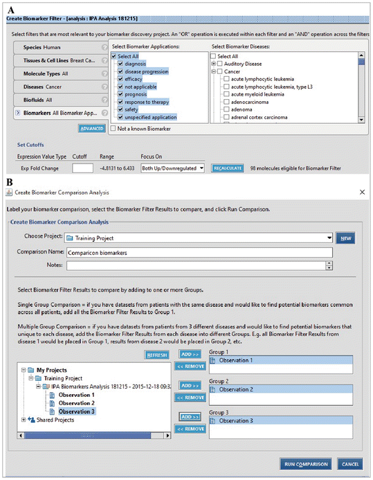
Filter parameters for biomarker analysis in IPA software. (a) Creating a filter for putative biomarkers. (b) Comparison analysis between all observations (MCF7, T47D and MDA-MB-231)
Full size image

We then ran the analysis, saved the results, and performed a comparative analysis on our datasets. In this analysis, we had three datasets to compare (Fig. 16.20b) and only considered proteins found in all three datasets. We found four candidate biomarkers common between the luminal A and Claudin-low cells falling into different biomarker application categories: unspecified application (↑KHSRP protein found in nucleus and ↓S100A8 with cytoplasmic localization), diagnosis, efficacy (↓RELA localized in nucleus and ↑STMN1 found in cytoplasm) RELA was also found related to the drug NF-kappa B decoy (Fig. 16.21). All proteins were found in blood and all are related to cancer; however, they are not unique to this disease, as they are found in other diseases.

8 Protein-Protein Interactions Databases

8.1 STRING

STRING (Search Tool for the Retrieval of Interacting Genes/Proteins) is a database of known and predicted protein interactions [31]. This database was developed by the Center for Protein Research (CPR), The European Molecular Biology Laboratory (EMBL), The Swiss Institute of Bioinformatics (SIB), The University of Copenhagen (KU), The Technische Universität Dresden (TUD), and The Universität Zürich (UZH). STRING version 10.0 has 9,643,763 proteins from 2031 organisms. The main objective of this database is to integrate, predict and unify several protein-protein interactions [31, 32]. Associations between proteins can be physical (direct) or functional (indirect). The functional associations are defined as the interaction between two proteins that participate or contribute in the same cellular process or metabolic pathway, as well as other functional processes [32–34].

STRING database uses the following type of information to predict possible interaction:

1.
Genomic data
2.
High throughput experiments
3.
Co-expression
4.
Data extracted from literature

STRING import knowledge about protein-protein interactions from other databases such as IntAct, MINT, BioGRID, Reactome, KEGG, BIND, HPRD, DIP, NCI-Nature Pathway Interaction, GO, and EcoCyc [33]. In addition, STRING has a large collection of predicted interactions that are produced de novo using prediction algorithms [33, 35]. De novo predictions are made using genomic context such as conserved genomic neighborhood, gene fusion events, and co-occurrence of genes across the genome [34]. STRING also performs searches for genes with similar transcriptional response through a variety of conditions (co-expression) [33]. Information extracted from literature is another source used to extract protein association information from. In this case, STRING obtains information from all abstracts in PubMed database directly [36]. Finally, STRING assigns a probabilistic confidence score to all associations obtained through comparison of the association predictions against a reference database. STRING uses the KEGG database because this is manually curated [32, 37].

STRING website is composed of two components, the first component deals with protein analysis and the second covers the platforms (Fig. 16.22). The window of results displays the networks of protein-protein associations. The resulting interactome is represented by connecting lines. Each one of these lines represents different types of evidence. Networks can be viewed in three forms:

1.
Evidence view in which connections are color coded as follows, neighborhood (green), gene fusion (red), co-occurrence (blue), co-expression (black), experiments (purple), database (light blue), text mining (yellow), and homology (gray)
2.
Confidence view in which the thickness of connecting lines correlates with the strength of the associations
3.
Interaction view in which the type of interactions is color coded as follows; activation (brilliant green), inhibition (red), binding (blue), phenotype (brilliant blue), catalysis (purple), posttranslational modifications (lilac), reaction (black) and expression (olive green)

STRING has also an interactive view. In this option the network can by reordered by moving the proteins in the network. In advanced option, the network can be enriched into a GO Biological Processes, GO Molecular functions, GO Cellular components, KEGG Pathways, PFAM domains, INTERPRO domains, and Protein- Protein interactions. In each enrichment category, a new window is displayed containing a list of interactors, which contains different processes, the number of proteins involved as well as a p- value.

8.2 Protein-Protein Interaction Networks

To determine the protein-protein interaction of overexpressed NUDC protein exclusively found in Claudin-low breast cancer cell line [18], we accessed the STRING website http://string-db.org/.

To generate a network of protein interactions, a list (one or more) of protein names, accession number, or sequence, as well as the organism or species they originated from, need to be specified (Fig. 16.22). At the bottom of the result window there is a parameter box. The options in the parameter box are used to select the active prediction algorithm. The confidence score as well as the number of interactors can be adjusted as well (Fig. 16.23). The interactome can be seen according to evidence (Fig. 16.24a), confidence (Fig. 16.24b) and action (Fig. 16.24c). In each network, a score is generated according to each protein’s interaction evidence. In addition, a brief description for each protein is also displayed (Fig. 16.24). NUDC protein is associated with PAFAH1B1 (platelet-activating factor acetylhydrolase 1b), PLK1 (polo-like kinase 1), NDEL1 (nudE nuclear distribution E homolog (A. nidulans)-like 1), HSP90AA1 (heat shock protein 90 kDa alpha), BTRC (beta-transducin repeat containing E3 ubiquitin protein ligase), NDE1 (nudE nuclear distribution E homolog 1 (A. nidulans)), ZW10 (ZW10, kinetochore associated, homolog (Drosophila), FBXW11 (F-box and WD repeat domain containing 11), CLIP1 (CAP-GLY domain containing linker protein 1) and ZWILCH (Zwilch, kinetochore associated, homolog (Drosophila)). All interactions have more than 0.90 score. In addition, the network was enriched into GO Biological Processes. Processes showed Enrichment with statistical significance were:

1.
Mitotic prometaphase (4.940 × 10⁻¹³)
2.
Mitotic anaphase (8.089 × 10⁻¹²)
3.
Mitotic M phase (6.309 × 10⁻¹¹)
4.
M phase (6.309 × 10⁻¹¹)
5.
Mitotic cell cycle phase (4.300 × 10⁻¹⁰)
6.
Cell cycle phase (4.300 × 10⁻¹⁰)

All processes mentioned above have at least eight proteins involved. We selected the cell cycle phase process as an example. The proteins enriched in this process are shown in color red (Fig. 16.25a). We selected the interacting proteins NUDC and ZW10 as examples to extract interaction information. ZW10 was selected because it is an essential component of the mitotic checkpoint that prevents cells from prematurely exiting mitosis. The evidence supporting the functional link between these two proteins are the following:

1.
Co-expression (putative homologs are co-expressed in other species, score 0.065)
2.
Association in curated database (score 0.900)
3.
Co-mentioned in PubMed abstracts (score 0.285)

Also putative homologs are mentioned together in other species (score 0.192). The combined score is 0.938. There is also activity evidence, such as catalysis (score 0.900), binding (score 0.900) and reaction (score of 0.900) that support the interaction between these two proteins (Fig. 16.25b). For proteins selected in a network, STRING displays a window with information about their 3D structure, as well as links to Ensembl, GeneCards, KEGG, Nextprot and UniProt. Also, STRING can show the protein sequence and the sequence of its homologs in organisms stored in STRING. NUDC has three 3D structures obtained from Protein DataBase (PDB) (Fig. 16.25c). As mentioned above, STRING can perform network analysis for multiple proteins as well. We performed an interactome analysis for the up- and down-regulated proteins common in Luminal A (MCF7 and T47D) and Claudin-low (MDA-MB-231) breast cancer cells lines [18]. In this case, we used the highest confidence (0.900) possible to generate our interaction network. The network has several interaction nodes related to:

1.
Energy metabolism
2.
Translation
3.
Proteasome
4.
Replication and repair
5.
Transcription

Red and green arrows indicate up- and down-regulated proteins, respectively (Fig. 16.26).

8.3 MINT

The Molecular INTeraction database or MINT is an open source protein-protein interaction database developed at the Università degli Studi di Roma Tor Vergata that has been experimentally verified [38, 39]. The webpage can be found at http://mint.bio.uniroma2.it/mint/Welcome.do (Fig. 16.27). The current version of MINT database (November 2015) contains 241,458 interactions, corresponding to 35,553 proteins and 5554 PMIDS (PubMed unique identifiers). Species included are Drosophila melanogaster, Saccharomyces cerevisiae, Caenorhabditis elegans, mammals and viruses, with mammal databases being the main datasets. Evidences for protein-protein interactions include association studies, co-localization, direct interactions, interactions in form of complexes, enzymatic reactions, and high throughput studies. Protein-protein interactions have been identified by a number of methods including co-immunoprecipitation with either anti-bait or anti-tag antibodies, fluorescence microscopy, peptide arrays, protein arrays, pull down experiments, SPR, tandem affinity isolation, two hybrid arrays, two hybrid pooling, and two hybrid systems, etc. Additionally, the MINT database is freely available for academic and commercial users.

There are three additional databases available via MINT website including HomoMINT, Domino, and VirusMINT. The first one is an inferred network for human; the second is specialized in domain-peptide interactions, and the last is a protein-protein interaction database specialized on viruses.

Protein interaction searches in MINT database (Fig. 16.28a) can be carried out using PubMed ID, D.O.I, or author’s name. Alternatively, this database can be searched against protein or gene name, protein accession number (Protein AN) or keywords. Protein accession numbers recognized by MINT search engine are FlyBase, Ensembl, Human Identified Gene Encoded Large Protein Analyzed database (HUGE), Nematode database (WormBase), OMIM, REACTOME pathway database, the Saccharomyces Genome Database (SGD), and Universal Protein Resource Knowledgebase (UniProtKB).

To demonstrate how MINT database works, we selected the vesicle-fusing ATPase NSF (P46459) for analysis. This protein is part of a set of proteins that were found overexpressed in several breast cancer cell lines [18]. To follow our analysis, click on the Search tab and type P46459 (Fig. 16.28, arrow 1) and then select the organism (Fig. 16.28, arrow 2) and then press the Search key (Fig. 16.28, arrow 3). Results show certain information for the queried protein including its ID, species, synonyms, domains found in query, a link to its role in diseases, its gene ontology, references covering the target protein, prediction of its modular domain interactions (ADAN), and its orthologs in MINT database (Fig. 16.28). Results also display a window containing a list of molecules interacting with the target according to MINT database, evidence for each interaction and a global score for each interaction (Fig. 16.28). Clicking on the MINT viewer will generate a list of interactions that are displayed as a function of score threshold. For each partner, a number showing evidence for interaction is shown (Fig. 16.29). As an example, we clicked on number 4 and a new window appeared showing the partner name, ID, and techniques used to determine the interaction, as well as a PubMed identifier containing this information (Fig. 16.29).

8.4 IntAct

IntAct is a database of protein-protein interactions, as well as a suite of analytical tools at The European Bioinformatics Institute (EBI), which is part of the European Molecular Biology Laboratory (EMBL) [40, 41]. All information has been curated by experts at the IntAct team.

This freely available database can be accessed through its webpage http://www.ebi.ac.uk/intact/.

As of November 26th, 2015 this database had registered 355,819 interactions, which included 89,340 interactors (proteins) described in 36,864 experiments, 13,892 PMIDs, and 564,831 binary interactions. Methods used for the determination of protein-protein interactions include tandem affinity purification, anti-tag co-immunoprecipitation, two hybrid systems, pull down experiments, two hybrid arrays, anti-bait co-immunoprecipitation, two hybrid pooling approach, and co-sedimentation, among others. The source of information mainly comes from human (42.5 %), various S. cerevisiae strains (22.8 %), Mus musculus (11.3 %), and D. melanogaster (8.1 %). Other species included are Escherichia coli, C. elegans, A. thaliana, Campylobacter jejuni, etc. MINT and IntAct databases have recently joined their individual efforts to optimize resources as the MIntAct project, thus avoiding duplication of activities [42].

IntAct model has three main components, interactions, interactors, and experiments used to determine interactions. Protein interactions are inferred using scientific publications, including binary interactions or complexes. An interactor can be defined as a biological molecule (mainly a protein) involved in a specific interaction. An interaction is not circumscribed to binary interactions only; it also includes interactions with more partners identified in the experiment performed, e.g. precipitation of multi-protein complexes. Search in IntAct database can be performed in different ways, including name of gene, protein, RNA or chemical compound, or UniProtKB, ChEBI (Chemical Entities of Biological Interest), RNA Central, PMID or IMEx (International Molecular Exchange) IDs. The principal page of IntAct (Fig. 16.30) contains links to other websites the might be of interest. These sites include MINT, UniProtKB, The Swiss Institute of Bioinformatics (SIB), The Interologous Interaction Database (I2D), The Innate Immune Response Database (Innate Database), Molecular Connections, The Extracellular Matrix Interactions Database (MatrixDB), The Modular Approach to Cellular Functions Resource (MB Info), a curated resource for functional analysis of agricultural plant and animal gene products (AgBase), and The cardiovascular Gene Annotation database at the London’s Global University (UCL).

As an example of the function of IntAct, we selected the protein XRCC6 (X-ray repair cross- complementing protein 6, UniProtKB ID P12956), which was found overexpressed in both Luminal A and MDA-MB-231 breast cancer cell lines [18]. This protein is a single-stranded DNA-dependent and ATP-dependent 3′–5′ DNA helicase involved in DNA non-homologous end joining (NHEJ) required for double-strand break repair and V(D)J recombination. To reproduce our analysis, in the search window (Fig. 16.30) type XRCC6 or P12956 ID and push the search key. A new window will appear on screen with the results for your query (Fig. 16.31). There are 324 binary interaction found for XRCC6 protein up to date. These interactions are displayed as a table, where molecule A is your query or bait, and B molecules are proteins interacting with your query. For each interaction, a list of interaction methods used for the determination of such interactions is shown, their corresponding IDs, and the source database as well. When you click on the interactors tab, a new page will be shown containing a list of all interactors, showing the type of interactor, the number of interactions described, a link to access the description in UniProtKB, and a description of the interaction (Fig. 16.32). More information, including interactions described, the chromosome location in Ensembl webpage, the mRNA expression for interactor in the Expression Atlas webpage, and pathways is displayed when interactors are searched separately. The map of interactions for your query can be displayed in three layouts, force directed (Fig. 16.33), radial (Fig. 16.34) or circle (Fig. 16.35). In all cases, you can zoom in the graph with the tool window at the bottom.

Search can also be performed for a list of identifiers. The result will be more complex as all interactions for each member of your list will be shown. As an example, we only show the graph for ten proteins overexpressed in Luminal A and MDA-MB-231 breast cancer cell lines [18], where a total of 1101 binary interactions were found in database (Figs. 16.36, 16.37 and 16.38).

8.5 HPRD

The Human Protein Reference Database (HPRD) is a free web resource containing information of human proteins, including an information summary for each protein, their PTMs, protein-protein interactions, expression levels in tissues, mRNA and protein sequences, non-protein interactions, alternate names, participation in diseases, and domains found in proteins. All the information stored in this database is curated by a group of expert biologists from the Pandey Lab at Johns Hopkins University and the Institute of Bioinformatics in Bangalore, India [43]. The current version of HPRD is 9. It contains information for 30,047 proteins, 41,327 protein-protein interactions, 93,710 PTMs, 112,158 sites of protein expression, 22,490 sites of intracellular localization, 470 domains, and 453,521 PMIDs. In addition, two other applications have been recently added, the PhosphoMotif Finder and NetPath resources, which allow the identification of phosphorylation motifs for known kinases/phosphatases and binding motifs for phospho serine/threonine or phospho tyrosine in a compendium of signaling pathways in humans [43].

To perform a search, click on the Query key, type your query and push the Search button on the upper left part on screen (Fig. 16.39, arrow). There are several options for a query, including Protein Name, Accession Number (RefSeq, GenBank, OMIM, UniProtKB and Entrez Gene Name), HPRD identifier, Gene Symbol, Chromosome locus, Molecular Class (e.g. Nuclease, Serine Proteinase, Translation Regulatory protein, Glycosylase, etc.), PTMs (e.g. ADP Ribosylation, Glycation, Nitration, Sumoylation. Ubiquitination), Cellular Component, Domain Name, Motif, Expression Site, Length of Protein sequence, Molecular Mass, and Diseases (Fig. 16.40). To present an example, we searched NUMA1. Results are shown in Fig. 16.41. Information retrieved includes the name of protein (NUMA1 corresponds to the Nuclear mitotic apparatus protein 1, isoform 1), Molecular Class (Structural protein), Molecular Function (Structural molecule activity), and Biological Process (Cell growth and/or maintenance). Seven additional tabs are provided, which are Summary, Sequence, Interactions, External Links, Alternate Names, Diseases, PTMs, and Substrates. The General tab contains the corresponding HPRD ID 01236, Gene symbol NUMA1, Molecular Weight 238259 Da, Chromosome location 11q13, intracellular localization, domains and motifs, and sites of tissue gene expression (Fig. 16.41). The sequence of NUMA1 and its corresponding mRNA are obtained by clicking on Sequence tab (Fig. 16.42). A list of proteins that interact with NUMA1, and types of experiment and interactions (direct or in a complex) are shown in Fig. 16.43.

Alternatively, it is possible to search HPRD by browsing Molecule Class, Domains, Motifs, PTMs, and Localization by pushing the Browse key on the right of the main webpage (Fig. 16.39). Furthermore, access to Human Proteinpedia, Pathways, PhosphoMotif Finder, or downloading the complete HPRD are possible using the main menu.

8.6 BioGRID

The Biological General Repository for Interaction Datasets (BioGRID, http://thebiogrid.org), as many other protein-protein interactions databases, has as main goals to curate, organize and make it freely available. The funding partners of this important database are the National Institutes of Health (NIH), the Canadian Institutes of Health Research (CIHR), the Genome Canada, and GenomeQuébec. Many other institutions have joined efforts to BioGRID, including the Université de Montréal, Princeton University, Mount Sinai Hospital, University of Edinburgh, SGD, FlyBase, GeneDB, NCBI, WormBase, MaizeGDB, MINT, IntAct, String, MatrixDB, SIB, GO, UniProt, Reactome, Cytoscape, and many others that can be found in the BioGRID webpage. The current version of BioGRID database (3.4.131, December 2015) has information for several model organisms, including A. thaliana, C. elegans, Candida albicans, Danio rerio, Dictyostellium discoideum, D. melanogaster, H. sapiens, Mus musculus, Neurospora crassa, Plasmodium falciparum, S. cerevisiae, Schizosaccharomyces pombe, Xenopus laevis, among other eukaryotic organisms. Furthermore, it has information of prokaryotic cells, such as B. subtilis, E. coli, Mycobacterium tuberculosis, and Streptococcus pneumoniae. Some viruses are included as well, e.g. Hepatitis C virus, Human Herpesvirus, Human Immunodeficiency virus, and Human Papillomavirus type 16 [44–46]. In its current version, the BioGRID database contains 749,213 non- redundant interactions, corresponding to 63,026 gene products and 45,623 unique publications. BioGRID database also includes 11,329 non-redundant interactions between 4851 unique chemical compounds and 2464 gene products accumulated from 8875 scientific publications. BioGRID also contains PTMs information. A total of 19,981 PTMs corresponding to 18,578 unassigned sites, 3165 unique proteins, 14,999 genes retrieved from 4317 publications are stored in this database.

To perform a search in BioGRID database, type your query (gene name, identifier or keywords) in the gene search window and select the species (Fig. 16.44). It is important to note that only one protein at a time can be searched. Alternatively, searches can be done by PubMed publication. However, searching of Multiple Genes or Publications will be available soon. As an example of a search, we selected the MCM6 protein, which was found overexpressed in both Luminal A and MDA-MB-231 breast cancer cell lines [18]. Results indicates that MCM6, the Minichromosome maintenance complex component 6, is involved in four GO Biological Processes:

1.
DNA replication
2.
DNA strand elongation involved in DNA replication
3.
G1/S transition of mitotic cell cycle
4.
Mitotic cell cycle

This protein is also involved in four GO Functions:

1.
ATP binding
2.
ATP-dependent DNA helicase activity
3.
Identical protein binding
4.
Protein binding

MCM6 is also part of three GO Components:

1.
MCM complex
2.
Nucleoplasm
3.
Nucleus (Fig. 16.45, arrows 1–3)

In order of significance according to the number of physical interactions, MCM6 has 82 interactors which are MCM2, MCM4, MCM7, MCM10, MCMBP, MCM3, CDT1, TONSL, MCM5, HIST1H4A, SSRP1, ASF1B, CDKN2A, ASF1A, MMS22L, and ING5 (Fig. 16.45). When the interactions option is selected, a list of 142 interactions are displayed on screen, indicating the name of interactor, its role in the interaction, name of the species, code for the experimental evidence, source of the dataset, whether interaction is from high or low high throughput screening experiments, a score for each interaction, the name of the person who curated the information, and additional notes (Fig. 16.46). When the Network tab is selected, three different layouts can be obtained: Concentric circles (Fig. 16.47), Single circle (Fig. 16.48), and Grid (Fig. 16.49). If the number of minimum evidence is changed to five for example, the number of interactions will drop (Fig. 16.50), thus reducing the complexity of the interaction map. When the PTM sites tab is selected, the amino acid sequence of the query is displayed and those residues with an identified PTM are highlighted in blue. Additional information such as the type of modification indicated as well as the source of information are also provided if PTM option is selected (Fig. 16.51). In the case of MCM6, there are 35 Lysine residues marked as ubiquitinated and two additional non-assigned PTMs (neddylation and sumoylation) (Fig. 16.52).

8.7 PIPs

The Human Protein-Protein Interaction Prediction (PIPs) is a specialized database containing a catalogue of predicted human protein-protein interactions that have been probabilistically determined using a Bayesian model, which takes into account several modules: Expression, Orthology, Localization, Domain co-occurrence, PTMs co-occurrence, Disorder, and Transitive. Expression considers information from a number of gene expression profiles. Orthology uses the interactions that have been determined for orthologues from fly, human, worm and yeast. Localization is determined by using a human subcellular localization predictor (PSLT) in different subcellular compartments. Domain co-occurrence uses the information stored in InterPro (Protein sequence analysis and classification, http://www.ebi.ac.uk/interpro) and Pfam (Protein families, http://pfam.xfam.org) protein domain databases. PTM co-occurrence uses the information contained in HPRD and UniProtKB. Disorder refers to the prediction of intrinsic disorder of protein found in VLS2 prediction. Finally, Transitive is a module which involves the local topology of networks, considering all modules described above [47].

PIPs database is located at the University of Dundee and the current version (December 2015) contains 37,606 interactions with a score > 1.0, indicating a high probability of occurrence. To perform a search, an ID in IPI, RefSeq or UniProtKB format must be entered in the search window. As an example, when TBP was used to initiate a query, results were displayed in several boxes each containing a number of interactions with a certain score. In this case, there are 65 interactions when a score value ≥ 1.0 was selected. For score values equal or larger than 2.5, 12.5, 25, 250, and 2500, there were 33, 15, 13, 7, and 3 interactions, respectively. When the number of interactions for a score ≥ 1.0 is selected, a list of interactors and the scores for each module used will be displayed on the screen.

8.8 MPIDB

The Microbial Protein Interaction Database (MPIDB) at the Craig Venter Institute (http://jcvi.org/mpidb/about.php) is a database whose main goal is to gather information for all known protein interactions from microbial organisms [48]. The current version of MPIDB is 2009-11-18 and contains 24,295 interactions that have been experimentally determined for 250 species of bacteria. This number of interactions corresponds to 7810 proteins and 24,295 interactors. Like many other databases, MPIDB also imports information from other databases, including IntAct, Database of Interacting Proteins (DIP), The Biomolecular Interaction Network Database (BIND) and MINT. Search can be performed using the name of a protein (UniProtKB ID or locus name) or by selecting species name. Results will be displayed as a table containing the UniProtKB ID, name of protein, interactor, loci of query and interactor, species for query and interactor and the number of evidences for such interaction.

8.9 TAIR

The Arabidopsis Information Resource (TAIR) at Phoenix Bioinformatics (https://www.arabidopsis.org) is a database of information for plant research model A. thaliana.

This database contains the whole A. thaliana genome sequence, analysis, structure and annotation of genes, information for all proteins encoded in its genome, data from gene expression experiments, genome maps, pathways, and other information useful to the scientific community [49]. Like other databases, experts from TAIR curate information using published experiments before entering them in this database. Search in TAIR can be performed in several ways: DNA/Clones, Ecotypes, Genes, Gene Ontology, Plant Ontology, Keywords, Locus, Markers, Microarray element, Microarray expression, People/Labs, Polymorphism/Alleles, Protein, Protocols, PMIDS, Seed/Germplasm, and Text. TAIR webpage also contains tools for analysis of sequences, as well as viewers for maps and sequences. It is recommended to register in TAIR to download the whole genome sequence.

8.10 GeneCards

The Human Gene Database (GeneCards, http://www.genecards.org) is another useful database covering the human genome [50–53]. This database was created by scientists at the Weizmann Institute of Science and LifeMap Sciences. Search can be done using keywords, symbols, aliases, or identifiers. Information that can be retrieved from this database include:

1.
Aliases for query
2.
Links to HGNC (HUGO Gene Nomenclature Committee, http://www.genenames.org), Entrez Gene at NCBI, Ensembl (genome databases for vertebrates and other eukaryotic species, http://www.ensembl.org/index.html), OMIM http://www.omim.org), and UniProtKB
3.
Summaries of queries retrieved from different sources
4.
Genomics data for query, including Regulatory Elements, Genomic location, Genomic region view, and RefSeq DNA sequence
5.
Protein information such as Protein ID, Length in amino acids, Molecular Mass, Quaternary structure, Three dimensional structure from OCA (Brower-database for protein structure/function, http://oca. weizmann.ac.il/oca-docs/oca-home.html) , Proteopedia (The free, collaborative D-encyclopedia of proteins & other molecules, http://proteopedia.org/wiki/index.php/Main_Page), Alternative splice forms, Data of protein expression in Proteomics DB (https://www.proteomicsdb.org/proteomicsdb/#overview), PaxDB (Protein Abundance Across Organisms, http://pax-db.org/#!home), MOPED (Multi-Omics Profiling Expression Database, https:// www.proteinspire.org/MOPED/mopedviews/ proteinExpressionDatabase.jsf), MaxQB (The MaxQuant DataBase, http://maxqb.biochem.mpg.de/mxdb/), and PTMs, (6) Domains in InterPro (Protein sequence, analysis and classification, http://www.ebi.ac.uk/interpro), ProtoNet (Automatic Hierarchical Classification of Proteins, http://www.protonet.cs.huji.ac.il/requested/cluster_card.php?global=protonet|no|6|61|lifetime|1|2|2&cluster=4023630&releaseid=6&firstEnterTimeClient=&blast=11053692|274977&clusteringNum=61)
6.
Functions retrieved from UniProtKB, Enzyme Number; Gene Ontology; Phenotypes; Animal models for query; links to CRISPR products, miRNAs, siRNAs, shRNAs, clone products, etc.
7.
Localization of genes in chromosomes and subcellular location of proteins
8.
Pathways
9.
Drugs for query
10.
Transcripts: Reference sequence (RefSeq), Enseml, Unigene Clusters
11.
Expression in tissues: GeneAnalytics (http://geneanalytics.genecards.org/?utm_source= genecards&utm_medium=banner&utm_ campaign=genecards&utm_content=banner_expression)
12.
Orthologs
13.
Paralogs
14.
Variants
15.
Disorders in MalaCards (The Humans Disease Database, http://www.malacards.org)
16.
Publications

In addition, there are a lot of links to companies that might have products for the protein of interests, such as antibodies, immunofluorescence, animal models, silencing, etc.

References

Kumar C, Mann M (2009) Bioinformatics analysis of mass spectrometry-based proteomics data sets. FEBS Lett 583(11):1703–1712
Article CAS PubMed Google Scholar
Su Z, Wang J, Yu J, Huang X, Gu X (2006) Evolution of alternative splicing after gene duplication. Genome Res 16(2):182–189
Article CAS PubMed PubMed Central Google Scholar
Twyman RM (2004) Principles of proteomics. Garland Biosciences/BIOS Scientific Publishers, Hampshire
Google Scholar
Ashburner M, Ball CA, Blake JA, Botstein D, Butler H, Cherry JM, Davis AP, Dolinski K, Dwight SS, Eppig JT et al (2000) Gene ontology: tool for the unification of biology. The gene ontology consortium. Nat Genet 25(1):25–29
Article CAS PubMed PubMed Central Google Scholar
Gene Ontology Consortium (2001) Creating the gene ontology resource: design and implementation. Genome Res 11(8):1425–1433
Article Google Scholar
Harris MA, Clark J, Ireland A, Lomax J, Ashburner M, Foulger R, Eilbeck K, Lewis S, Marshall B, Mungall C et al (2004) The Gene Ontology (GO) database and informatics resource. Nucleic Acids Res 32(Database issue):D258–D261
CAS PubMed Google Scholar
Gene Ontology C (2015) Gene ontology consortium: going forward. Nucleic Acids Res 43(Database issue):D1049–D1056
Article Google Scholar
Rhee SY, Wood V, Dolinski K, Draghici S (2008) Use and misuse of the gene ontology annotations. Nat Rev Genet 9(7):509–515
Article CAS PubMed Google Scholar
Mi H, Muruganujan A, Casagrande JT, Thomas PD (2013) Large-scale gene function analysis with the PANTHER classification system. Nat Protoc 8(8):1551–1566
Article PubMed Google Scholar
Thomas PD, Campbell MJ, Kejariwal A, Mi H, Karlak B, Daverman R, Diemer K, Muruganujan A, Narechania A (2003) PANTHER: a library of protein families and subfamilies indexed by function. Genome Res 13(9):2129–2141
Article CAS PubMed PubMed Central Google Scholar
Thomas PD, Kejariwal A, Campbell MJ, Mi H, Diemer K, Guo N, Ladunga I, Ulitsky- Lazareva B, Muruganujan A, Rabkin S et al (2003) PANTHER: a browsable database of gene products organized by biological function, using curated protein family and subfamily classification. Nucleic Acids Res 31(1):334–341
Article CAS PubMed PubMed Central Google Scholar
Mi H, Lazareva-Ulitsky B, Loo R, Kejariwal A, Vandergriff J, Rabkin S, Guo N, Muruganujan A, Doremieux O, Campbell MJ et al (2005) The PANTHER database of protein families, subfamilies, functions and pathways. Nucleic Acids Res 33(Database issue):D284–D288
Article CAS PubMed Google Scholar
Funahashi A, Jouraku A, Matsuoka Y, Morohashi M, Kikuchi N, Kitano H (2008) CellDesigner 3.5: a versatile modeling tool for biochemical networks. Proc IEEE 96(8):1254
Article Google Scholar
Mi H, Guo N, Kejariwal A, Thomas PD (2007) PANTHER version 6: protein sequence and function evolution data with expanded representation of biological pathways. Nucleic Acids Res 35(Database issue):D247–D252
Article CAS PubMed Google Scholar
Mi H, Thomas P (2009) PANTHER pathway: an ontology-based pathway database coupled with data analysis tools. Methods Mol Biol 563:123–140
Article CAS PubMed Google Scholar
PANTHER User Manual (2015). http://pantherdb.org/help/PANTHER_user_manual.pdf
Mi H, Muruganujan A, Thomas PD (2013) PANTHER in 2013: modeling the evolution of gene function, and other gene attributes, in the context of phylogenetic trees. Nucleic Acids Res 41(Database issue):D377–D386
Article CAS PubMed Google Scholar
Calderon-Gonzalez KG, Valero Rustarazo ML, Labra-Barrios ML, Bazan-Mendez CI, Tavera-Tapia A, Herrera-Aguirre M, Sanchez Del Pino MM, Gallegos-Perez JL, Gonzalez- Marquez H, Hernandez-Hernandez JM et al (2015) Data set of the protein expression profiles of Luminal A, Claudin-low and overexpressing HER2(+) breast cancer cell lines by iTRAQ labelling and tandem mass spectrometry. Data Brief 4:292–301
Article PubMed PubMed Central Google Scholar
Dennis G Jr, Sherman BT, Hosack DA, Yang J, Gao W, Lane HC, Lempicki RA (2003) DAVID: database for annotation, visualization, and integrated discovery. Genome Biol 4(5):P3
Article PubMed Google Scholar
da Huang W, Sherman BT, Lempicki RA (2009) Bioinformatics enrichment tools: paths toward the comprehensive functional analysis of large gene lists. Nucleic Acids Res 37(1):1–13
Article Google Scholar
Huang DW, Sherman BT, Tan Q, Kir J, Liu D, Bryant D, Guo Y, Stephens R, Baseler MW, Lane HC et al (2007) DAVID bioinformatics resources: expanded annotation database and novel algorithms to better extract biology from large gene lists. Nucleic Acids Res 35(Web Server issue):W169–W175
Article PubMed PubMed Central Google Scholar
da Huang W, Sherman BT, Lempicki RA (2009) Systematic and integrative analysis of large gene lists using DAVID bioinformatics resources. Nat Protoc 4(1):44–57
Article CAS Google Scholar
da Huang W, Sherman BT, Stephens R, Baseler MW, Lane HC, Lempicki RA (2008) DAVID gene ID conversion tool. Bioinformation 2(10):428–430
Article PubMed Central Google Scholar
Kanehisa M, Goto S, Kawashima S, Okuno Y, Hattori M (2004) The KEGG resource for deciphering the genome. Nucleic Acids Res 32(Database issue):D277–D280
Article CAS PubMed PubMed Central Google Scholar
Kanehisa M, Goto S, Hattori M, Aoki-Kinoshita KF, Itoh M, Kawashima S, Katayama T, Araki M, Hirakawa M (2006) From genomics to chemical genomics: new developments in KEGG. Nucleic Acids Res 34(Database issue):D354–D357
Article CAS PubMed Google Scholar
Kanehisa M, Sato Y, Kawashima M, Furumichi M, Tanabe M (2015) KEGG as a reference resource for gene and protein annotation. Nucleic Acids Res 44:457
Article Google Scholar
Kanehisa M, Sato Y, Morishima K (2015) BlastKOALA and GhostKOALA: KEGG tools for functional characterization of genome and metagenome sequences. J Mol Biol 428:726
Article PubMed Google Scholar
Kanehisa M, Goto S, Sato Y, Furumichi M, Tanabe M (2012) KEGG for integration and interpretation of large-scale molecular data sets. Nucleic Acids Res 40(Database issue):D109–D114
Article CAS PubMed Google Scholar
Okuda S, Yamada T, Hamajima M, Itoh M, Katayama T, Bork P, Goto S, Kanehisa M (2008) KEGG Atlas mapping for global analysis of metabolic pathways. Nucleic Acids Res 36(Web Server issue):W423–W426
Article CAS PubMed PubMed Central Google Scholar
Chaiboonchoe A, Samarasinghe S, Kulasiri D, Salehi-Ashtiani K (2014) Integrated analysis of gene network in childhood leukemia from microarray and pathway databases. BioMed Res Int 2014:278748
Article PubMed PubMed Central Google Scholar
von Mering C, Jensen LJ, Kuhn M, Chaffron S, Doerks T, Kruger B, Snel B, Bork P (2007) STRING 7--recent developments in the integration and prediction of protein interactions. Nucleic Acids Res 35(Database issue):D358–D362
Article Google Scholar
von Mering C, Jensen LJ, Snel B, Hooper SD, Krupp M, Foglierini M, Jouffre N, Huynen MA, Bork P (2005) STRING: known and predicted protein-protein associations, integrated and transferred across organisms. Nucleic Acids Res 33(Database issue):D433–D437
Article Google Scholar
Jensen LJ, Kuhn M, Stark M, Chaffron S, Creevey C, Muller J, Doerks T, Julien P, Roth A, Simonovic M et al (2009) STRING 8--a global view on proteins and their functional interactions in 630 organisms. Nucleic Acids Res 37(Database issue):D412–D416
Article CAS PubMed Google Scholar
von Mering C, Huynen M, Jaeggi D, Schmidt S, Bork P, Snel B (2003) STRING: a database of predicted functional associations between proteins. Nucleic Acids Res 31(1):258–261
Article Google Scholar
Harrington ED, Jensen LJ, Bork P (2008) Predicting biological networks from genomic data. FEBS Lett 582(8):1251–1258
Article CAS PubMed Google Scholar
Marcotte EM, Xenarios I, Eisenberg D (2001) Mining literature for protein-protein interactions. Bioinformatics 17(4):359–363
Article CAS PubMed Google Scholar
Szklarczyk D, Franceschini A, Kuhn M, Simonovic M, Roth A, Minguez P, Doerks T, Stark M, Muller J, Bork P et al (2011) The STRING database in 2011: functional interaction networks of proteins, globally integrated and scored. Nucleic Acids Res 39(Database issue):D561–D568
Article CAS PubMed Google Scholar
Zanzoni A, Montecchi-Palazzi L, Quondam M, Ausiello G, Helmer-Citterich M, Cesareni G (2002) MINT: a molecular INTeraction database. FEBS Lett 513(1):135–140
Article CAS PubMed Google Scholar
Licata L, Briganti L, Peluso D, Perfetto L, Iannuccelli M, Galeota E, Sacco F, Palma A, Nardozza AP, Santonico E et al (2012) MINT, the molecular interaction database: 2012 update. Nucleic Acids Res 40(Database issue):D857–D861
Article CAS PubMed Google Scholar
Hermjakob H, Montecchi-Palazzi L, Lewington C, Mudali S, Kerrien S, Orchard S, Vingron M, Roechert B, Roepstorff P, Valencia A et al (2004) IntAct: an open source molecular interaction database. Nucleic Acids Res 32(Database issue):D452–D455
Article CAS PubMed PubMed Central Google Scholar
Kerrien S, Alam-Faruque Y, Aranda B, Bancarz I, Bridge A, Derow C, Dimmer E, Feuermann M, Friedrichsen A, Huntley R et al (2007) IntAct--open source resource for molecular interaction data. Nucleic Acids Res 35(Database issue):D561–D565
Article CAS PubMed Google Scholar
Orchard S, Ammari M, Aranda B, Breuza L, Briganti L, Broackes-Carter F, Campbell NH, Chavali G, Chen C, del-Toro N et al (2014) The MIntAct project--IntAct as a common curation platform for 11 molecular interaction databases. Nucleic Acids Res 42(Database issue):D358–D363
Article CAS PubMed Google Scholar
Keshava Prasad TS, Goel R, Kandasamy K, Keerthikumar S, Kumar S, Mathivanan S, Telikicherla D, Raju R, Shafreen B, Venugopal A et al (2009) Human protein reference database--2009 update. Nucleic Acids Res 37(Database issue):D767–D772
Article CAS PubMed Google Scholar
Breitkreutz BJ, Stark C, Tyers M (2003) The GRID: the general repository for interaction datasets. Genome Biol 4(3):R23
Article PubMed PubMed Central Google Scholar
Stark C, Breitkreutz BJ, Reguly T, Boucher L, Breitkreutz A, Tyers M (2006) BioGRID: a general repository for interaction datasets. Nucleic Acids Res 34(Database issue):D535–D539
Article CAS PubMed Google Scholar
Chatr-Aryamontri A, Breitkreutz BJ, Oughtred R, Boucher L, Heinicke S, Chen D, Stark C, Breitkreutz A, Kolas N, O’Donnell L et al (2015) The BioGRID interaction database: 2015 update. Nucleic Acids Res 43(Database issue):D470–D478
Article PubMed Google Scholar
Scott MS, Barton GJ (2007) Probabilistic prediction and ranking of human protein-protein interactions. BMC Bioinf 8:239
Article Google Scholar
Goll J, Rajagopala SV, Shiau SC, Wu H, Lamb BT, Uetz P (2008) MPIDB: the microbial protein interaction database. Bioinformatics 24(15):1743–1744
Article CAS PubMed PubMed Central Google Scholar
Lamesch P, Berardini TZ, Li D, Swarbreck D, Wilks C, Sasidharan R, Muller R, Dreher K, Alexander DL, Garcia-Hernandez M et al (2012) The Arabidopsis Information Resource (TAIR): improved gene annotation and new tools. Nucleic Acids Res 40(Database issue):D1202–D1210
Article CAS PubMed Google Scholar
Rebhan M, Chalifa-Caspi V, Prilusky J, Lancet D (1997) GeneCards: integrating information about genes, proteins and diseases. Trends Genet 13(4):163
Article CAS PubMed Google Scholar
Safran MC-CV, Shmueli O, Rosen N, Benjamin-Rodrig H, Ophir R, Yanai I, Shmoish M, Lancet D (2003) The GeneCards family of databases: GeneCards, GeneLoc, GeneNote and GeneAnnot. In: Proceedings of the IEEE Computer Science Bioinformatics Conference CSB2003
Google Scholar
Stelzer GHA, Dalah A, Rosen N, Shmoish M, Iny Stein T, Sirota A, Madi A, Safran M, Lancet D (2008) GeneCards: one stop site for human gene research. FISEB (ILANIT)
Google Scholar
Harel A, Inger A, Stelzer G, Strichman-Almashanu L, Dalah I, Safran M, Lancet D (2009) GIFtS: annotation landscape analysis with GeneCards. BMC Bioinf 10:348
Article Google Scholar

Download references

Acknowledgements

We thank the Instituto de Ciencia y Tecnología del Distrito Federal (ICyTDF), now renamed Secretaría de Ciencia, Tecnología e Innovación de la Ciudad de México (SECITI), for its support with the project ICyTDF-J.LA (CM-272/12-SECITI/033/2012), and Consejo Nacional de Ciencia y Tecnología (Conacyt) from Mexico, with the project number SALUD-2009-01-113674, both granted to Dr. Juan Pedro Luna Arias.

Author information

Authors and Affiliations

Departamento de Biología Celular, Centro de Investigación y de Estudios Avanzados del Instituto Politécnico Nacional (Cinvestav-IPN), Av. Instituto Politécnico Nacional 2508, Col. San Pedro Zacatenco, Gustavo A. Madero, C.P. 07360, Ciudad de México, Mexico
Karla Grisel Calderón-González, María Esther Herrera-Aguirre & Juan Pedro Luna-Arias
Instituto de Física, Universidad Autónoma de San Luis Potosí, Av. Manuel Nava 6, Zona Universitaria, C.P. 78290, San Luis Potosí, S.L.P., Mexico
Jesús Hernández-Monge

Authors

Karla Grisel Calderón-González
View author publications
You can also search for this author in PubMed Google Scholar
Jesús Hernández-Monge
View author publications
You can also search for this author in PubMed Google Scholar
María Esther Herrera-Aguirre
View author publications
You can also search for this author in PubMed Google Scholar
Juan Pedro Luna-Arias
View author publications
You can also search for this author in PubMed Google Scholar

Corresponding author

Correspondence to Juan Pedro Luna-Arias .

Editor information

Editors and Affiliations

UT Southwestern Medical Center, Dallas, Texas, USA
Hamid Mirzaei
Biotech Division, Neurophagy Therapeutics, INC, Odessa, Texas, USA
Martin Carrasco

Rights and permissions

Reprints and permissions

Copyright information

About this chapter

Cite this chapter

Calderón-González, K.G., Hernández-Monge, J., Herrera-Aguirre, M.E., Luna-Arias, J.P. (2016). Bioinformatics Tools for Proteomics Data Interpretation. In: Mirzaei, H., Carrasco, M. (eds) Modern Proteomics – Sample Preparation, Analysis and Practical Applications. Advances in Experimental Medicine and Biology, vol 919. Springer, Cham. https://doi.org/10.1007/978-3-319-41448-5_16

Download citation

DOI: https://doi.org/10.1007/978-3-319-41448-5_16
Published: 15 December 2016
Publisher Name: Springer, Cham
Print ISBN: 978-3-319-41446-1
Online ISBN: 978-3-319-41448-5
eBook Packages: Biomedical and Life SciencesBiomedical and Life Sciences (R0)

Publish with us

Policies and ethics

Bioinformatics Tools for Proteomics Data Interpretation

Abstract

Similar content being viewed by others

Bioinformatics Resources

Proteogenomics: concepts, applications and computational strategies

Omics: Data Processing and Analysis

Keywords

1 Gene Ontology

2 PANTHER

3 PANTHER Gene List Analysis

4 DAVID

5 KEGG

Pathway Maps Analysis

6 Ingenuity Pathway Analysis (IPA)

7 Biomarkers Module

8 Protein-Protein Interactions Databases

8.1 STRING

8.2 Protein-Protein Interaction Networks

8.3 MINT

8.4 IntAct

8.5 HPRD

8.6 BioGRID

8.7 PIPs

8.8 MPIDB

8.9 TAIR

8.10 GeneCards

References

Acknowledgements

Author information

Authors and Affiliations

Corresponding author

Editor information

Editors and Affiliations

Rights and permissions

Copyright information

About this chapter

Cite this chapter

Download citation

Publish with us

Navigation

Bioinformatics Tools for Proteomics Data Interpretation

Abstract

Similar content being viewed by others

Bioinformatics Resources

Proteogenomics: concepts, applications and computational strategies

Omics: Data Processing and Analysis

Keywords

1 Gene Ontology

2 PANTHER

3 PANTHER Gene List Analysis

4 DAVID

5 KEGG

Pathway Maps Analysis

6 Ingenuity Pathway Analysis (IPA)

7 Biomarkers Module

8 Protein-Protein Interactions Databases

8.1 STRING

8.2 Protein-Protein Interaction Networks

8.3 MINT

8.4 IntAct

8.5 HPRD

8.6 BioGRID

8.7 PIPs

8.8 MPIDB

8.9 TAIR

8.10 GeneCards

References

Acknowledgements

Author information

Authors and Affiliations

Corresponding author

Editor information

Editors and Affiliations

Rights and permissions

Copyright information

About this chapter

Cite this chapter

Download citation

Share this chapter

Publish with us

Search

Navigation