Modelling of Floating Offshore Wind Technologies

Matha, Denis; Cruz, Joao; Masciola, Marco; Bachynski, Erin E.; Atcheson, Mairéad; Goupee, Andrew J.; Gueydon, Sébastien M. H.; Robertson, Amy N.

doi:10.1007/978-3-319-29398-1_4

Denis Matha³,
Joao Cruz⁴,
Marco Masciola⁵,
Erin E. Bachynski⁶,
Mairéad Atcheson⁴,
Andrew J. Goupee⁷,
Sébastien M. H. Gueydon⁸ &
…
Amy N. Robertson⁹

Part of the book series: Green Energy and Technology ((GREEN))

3204 Accesses
1 Citations

Abstract

The modelling of FOWT forms a critical stage of the design process, as it allows a fully coupled dynamic assessment of the response of the concept while accounting for blade-rotor dynamics, support structure motions and mooring dynamics. For both new and for existing concepts, modelling offers the potential to test, in controlled environments, a series of assumptions and scenarios at a relatively minor cost. Two fundamental modelling approaches can be followed: numerical and experimental.

Access provided by Autonomous University of Puebla. Download chapter PDF

Multibody modeling for concept-level floating offshore wind turbine design

Article Open access 27 February 2020

Hydro- and aero-elastic response of floating offshore wind turbines to combined waves and wind in frequency domain

Article Open access 16 March 2024

Development of a fully coupled aero-hydro-mooring-elastic tool for floating offshore wind turbines

Article 21 January 2019

Keywords

These keywords were added by machine and not by the authors. This process is experimental and the keywords may be updated as the learning algorithm improves.

The modelling of FOWT forms a critical stage of the design process, as it allows a fully coupled dynamic assessment of the response of the concept while accounting for blade-rotor dynamics, support structure motions and mooring dynamics. For both new and for existing concepts, modelling offers the potential to test, in controlled environments, a series of assumptions and scenarios at a relatively minor cost. Two fundamental modelling approaches can be followed: numerical and experimental. The former carries the potential to allow a wider range of design iterations and design situations to be tested at a low cost and under a potentially shorter timeframe, while the latter may prove useful for specific physical tests outside the remit of existing numerical tools and/or to validate early numerical estimates. In this chapter the main physical aspects to be modelled are described in detail: firstly, the key considerations regarding aerodynamics (Sect. 1) and hydrodynamics (Sect. 2) are described, in an effort to overview the main options that a design engineer may wish follow when considering the modelling of FOWT. In addition, specific aspects related to the assessment of the mooring dynamics and the structural design of FOWTs are also detailed in Sects. 3 and 4, respectively. Finally, the chapter is concluded with a brief overview of the available numerical tools that specifically address FOWT modelling (Sect. 5), and with a detailed case study related to the experimental testing of a FOWT (Sect. 6).

1 Aerodynamics

Denis Matha

1.1 Introduction

The primary purpose of a wind turbine on a floating support structure is to extract kinetic energy from the incoming wind by the rotor to generate electricity, as it is the case for bottom-fixed and onshore wind turbines. While the aerodynamic principles and mechanisms are the same, the additional degrees of freedom of a FOWT may influence the aerodynamics of the rotor and of the airfoil sections along the blade. This section will provide an introduction into wind turbine aerodynamics and common methodologies to calculate the aerodynamic forces on rotor blades in general and will be concluded by a summary of the particular challenges in aerodynamics of FOWTs.

1.2 Wind Turbine Rotor Aerodynamics Basics

The energy $ P_{max} $ that can be extracted by a wind turbine rotor is given by the expression:

$$ P_{max} = \frac{1}{2}C_{p} \rho AU_{{\infty }}^{3} $$

(1)

where $ \rho $ is the air density, A the rotor swept area, $ U_{{\infty }} $ the wind speed perpendicular to the rotor plane far in front of the rotor and $ C_{p} $ the power coefficient, which is limited by the Betz limit $ C_{{P_{max} }} = \frac{16}{27} \approx 0.593. $ The Betz limit can be derived by application of classical momentum theory applied on a 1D control volume as depicted in Fig. 1:

$$ \frac{\partial }{\partial t}\mathop{{\int\!\!\!\!\!\int\!\!\!\!\!\int}\mkern-31.2mu \bigodot}\limits_{CV} {\rho \vec{v}dV} + \mathop{{\int\!\!\!\!\!\int}\mkern-21mu \bigcirc}\limits_{S} {\rho \vec{v}\left( {\vec{v} \cdot \vec{n}} \right)dS = \vec{F}} $$

(2)

Assuming stationary flow $ \frac{{\partial }}{{{\partial }t}} = 0 $ and considering that net external pressure force on the control volume is zero because the control volume is surrounded by ambient pressure $ p_{{\infty }} $, the equation simplifies to:

$$ - \rho U_{{\infty }}^{2} A_{1} + \rho U_{w}^{2} A_{2} = - T $$

(3)

By application of the Bernoulli equation in front of and after the pressure drop $ \Delta p $ at the rotor disc (Eq. 4) and utilizing the law of conservation of mass (Eq. 5), one can derive the thrust (Eq. 6) and power output (Eq. 7) (from the integral energy balance of the control volume) of the turbine as:

$$ \Delta p = \frac{1}{2}\rho \left( {U_{{\infty }}^{2} - U_{w}^{2} } \right) $$

(4)

$$ \dot{m} = \rho UA = \rho U_{{\infty }} A_{1} = \rho U_{w} A_{2} $$

(5)

$$ T = \rho UA\left( {U_{{\infty }} - U_{w} } \right) $$

(6)

$$ P = T \cdot U = \frac{1}{2}\rho UA\left( {U_{\infty }^{2} - U_{w}^{2} } \right) $$

(7)

In wind energy the axial induction factor a is introduced to describe the velocity deficit caused by the flow deceleration in the rotor plane:

$$ u_{i} = aU_{{\infty }} $$

(8)

with $ u_{i} $ denominated as the induced velocity. Using the induction factor relationships from Eqs. (9) and (10) below, Eq. (7) can be rewritten as Eq. (11):

$$ {\text{U}} = \left( {1 - {\text{a}}} \right){\text{U}}_{{\infty }} $$

(9)

$$ {\text{U}}_{\text{w}} = \left( {1 - 2{\text{a}}} \right){\text{U}}_{{\infty }} $$

(10)

$$ P = T \cdot U = 2\rho U_{{\infty }}^{3} {\text{A}} \cdot {\text{a}}\left( {1 - {\text{a}}} \right)^{2} $$

(11)

It is important to note in particular with regard to floating wind turbines as described in the next section, that Eq. (11) assumes momentum balance, which is only valid up to an induction factor, an induced velocity of

$$ {\text{a}} \le 0.5,\quad {\text{respectively}}\;\;U_{{\infty }} \ge 2\left| {u_{i} } \right| $$

(12)

If $ a > 0.5 $, then Eq. (10) predicts $ U_{w} < 0 $ which would mean an unphysical flow reversal in the wake. In reality, additional air is sucked into the wake from the surrounding flow by developing eddies; i.e. momentum is transported from the outer flow into the control volume rendering the momentum balance assumption invalid.

When the air passes through the rotor and part of its kinetic energy is transformed into the electricity-producing shaft torque, the basic laws of Newtonian Mechanics imply that an opposite and equal reaction torque must be imposed on the wake. This wake rotation velocity component $ V_{\Omega } $ at a radial rotor distance r, which is directed tangential to the rotor rotation, is expressed in terms of a tangential induction factor $ a^{{\prime }} $:

$$ V_{\Omega } = 2r\Omega a^{{\prime }} $$

(13)

The torque $ \Delta Q $ on a rotor annulus (annular ring) at radius r and width $ \Delta r $ generated by the change of the angular momentum in the wake can be expressed as:

$$ \Delta Q = \rho 2\pi r^{2} U_{{\infty }} \left( {1 - a} \right)V_{\Omega }\Delta r $$

(14)

Equating the resulting rotor shaft power (Eq. 14) with the power derived from the axial momentum analysis (Eq. 11) yields a relationship between axial and tangential induction factor with the so-called dimensionless local tip-speed ratio $ TSR_{local} $ (for completeness, the often used global tip-speed ratio TSR, computed for the outer rotor radius R is also given here):

$$ \Delta P =\Delta Q \cdot\Omega $$

(15)

$$ TSR_{local} = \frac{{r\Omega }}{{U_{{\infty }} }},\quad TSR = \frac{{R\Omega }}{{U_{{\infty }} }} $$

(16)

$$ a\left( {1 - a} \right) = TSR_{local}^{2} a^{{\prime }} $$

(17)

1.3 Blade Element Momentum Method

The most widely used technique to compute the aerodynamic power of a wind turbine rotor is the blade element momentum method, commonly abbreviated by BEM. It combines the previously outlined momentum analysis in axial and tangential direction with the local blade element theory, which relates the aerodynamic lift $ \vec{L} $ and drag $ \vec{D} $ forces acting on a blade element of width $ \Delta r $ and chord length c to the incoming flow velocity $ \vec{V} $:

$$ \Delta \vec{L} = \frac{1}{2}C_{l} \rho \vec{V}^{2} c\Delta r,\quad \vec{L}\parallel \vec{V} $$

(18)

$$ \Delta \vec{D} = \frac{1}{2}C_{d} \rho \vec{V}^{2} c\Delta r,\quad \vec{D} \bot \vec{V} $$

(19)

The lift coefficient $ C_{l} $ and drag coefficient $ C_{d} $ are functions of the angle of attack $ \alpha $ and the Reynolds number Re and are also sensitive to surface roughness, i.e. pollution and deterioration of the blade surface e.g. by salt water. They are typically known from wind tunnel measurements or computations for 2D airfoils.

$$ C_{l} , C_{d} = f\left( {\alpha ,Re} \right) $$

(20)

Figure 2 depicts the geometric relationships at a blade element, with the angle of attack $ \alpha = \varphi - \beta $, blade chord angle $ \beta $ (typically the of sum built-in blade twist and current pitch angle) and the inflow angle $ \varphi $.

From Fig. 1 it follows, that for a blade element at radius r, the inflow angle can be computed as:

$$ \tan {\upvarphi } = \frac{{U_{{\infty }} \left( {1 - a} \right)}}{{\Omega r\left( {1 + a^{{\prime }} } \right)}} $$

(21)

Dividing the rotor into multiple annuli of width $ \Delta r $, i.e. discretising the blade into multiple elements, the basic BEM algorithm can be derived by balancing the following thrust and torque equations on each annulus derived from the blade element method (BE) and from the momentum analysis (MA):

$$ \Delta T_{MA} = 4\pi r\rho U_{\infty }^{2} a\left( {1 - a} \right)\Delta r $$

(22)

$$ \Delta Q_{MA} = 4\pi r^{3} \rho U_{\infty }\Omega a^{{\prime }} \left( {1 - a} \right)\Delta r $$

(23)

$$ \Delta T_{BE} = n\left( {L\left( {C_{l} } \right)\cos \varphi + D\left( {C_{d} } \right)\sin \varphi } \right)\Delta r $$

(24)

$$ \Delta Q_{BE} = n\left( {L\left( {C_{l} } \right)\sin \varphi - D\left( {C_{d} } \right)\cos \varphi } \right)r\Delta r $$

(25)

With these equations, the classical BEM algorithm can be established. In Table 1, a scheme for a typical BEM algorithm is described (steps 1–6 without the steps marked with superscript *). In addition to the previously described basic relations, most modern BEM implementations account for aerodynamic effects that are not captured with the outlined underlying basic theory by applying engineering correction models. These empirical or semi-empirical models are also included in Table 1. Further details on these correction models, as well as the BEM method in general is found e.g. in Sant (2007) and Moriarty and Hansen (2005).

Table 1 BEM algorithm with correction models (note that the position of the correction models in the stepwise algorithm may be different than shown here depending on the specific software implementation and correction model used)

Full size table

1.4 Potential Flow and CFD Methods

So far the focus was on BEM theory, because it is by far the most widely used aerodynamic method to compute aerodynamic loads on wind turbine rotors. Nevertheless, there are certain limitation in BEM theory that can only be addressed by application of engineering correction models, as presented in Table 1. With increasing computational power available, more computationally expensive aerodynamic models are developed and applied to overcome BEM limitations. The most important two methods are:

Potential flow, and
Computational fluid dynamics (CFD) based methods.

Potential flow methods are based on the assumptions of incompressible, irrotational, inviscid flow. The most fundamental equations for potential flow methods are the Laplace equation (Eq. 26) for the velocity potential $ \varphi $; the Biot Savart law (Eq. 27) establishing a relation for the induced velocity from a vortex filament dl with circulation strength $ \Gamma $ to an arbitrary point at distance r; the Kutta-Joukowski theorem (Eq. 28), linking the lift force from blade element theory to the circulation strength and Kelvin’s circulation theorem (Eq. 29) stating that the circulation in the domain must remain constant in time. In addition, the Helmholtz theorem needs to be fulfilled which demands that a bound vortex filament cannot start or end abruptly in the domain, resulting in the typical horseshoe shaped lattice structure.

$$ {\nabla }^{2} \varphi = 0 $$

(26)

$$ {\text{dU}} = - \frac{\Gamma }{{4\uppi}}\frac{r \times dl}{{\left| r \right|^{3} }} $$

(27)

$$ \Delta \vec{L}\left( r \right) = \frac{1}{2}C_{l} \rho \vec{V}^{2} c\Delta r = \rho V\Gamma \left( r \right) $$

(28)

$$ \frac{{D\Gamma }}{DT} = 0 $$

(29)

In the most widely applied potential flow method for wind turbine applications based on the lifting line free vortex wake theory, the rotor blade is discretised into several segments, each with its individual bound circulation strength. From these nodes at the blade, over time vortex filaments are evolving into a vortex lattice representing the complex wake structure, with trailing filaments (directed in the local velocity direction) related to the spanwise spatial bound circulation gradients $ \partial\Gamma /\partial x $ and shed filaments (parallel to the bound filaments) related to temporal variation of bound circulation strength $ \partial\Gamma /\partial t $. The Biot-Savart law is used to compute the velocity induced by the wake on each node, while the Kutta-Joukowski theorem is applied to compute the bound vorticity strength along the blade span depending on the current inflow velocity and direction at each blade segment. In Leishman (2006), Sebastian (2012) detailed information on the approach can be found. The advantage of this method compared to BEM is that the rotor wake is physically modeled in space and time and phenomena like tip roll-up, the dynamic inflow effect and rotor motions into and out of the wake as potentially present for FOWTs are represented without additional engineering correction models.

Computational fluid dynamics (CFD) models are based on the Navier Stokes Equations (NSE) for which no analytical solution has been found yet and which therefore need to be solved numerically (for brevity the NSE are not presented here, see e.g. Anderson (2007) for further details). The most widely used approximation of the NSE for wind turbine rotor aerodynamic load calculations is based on the Reynolds averaged NSE (RANS) for modelling of turbulent flows. By decomposing the NSE into time-averaged and fluctuating quantities, a nonlinear Reynolds stress term is generated that requires additional turbulence models to close the RANS equation for solving. The RANS equations are typically discretised by either finite differences, finite volumes or finite elements methods, with the computational domain spatially discretised by structured or unstructured meshes. Another approach that is also applied for wind turbine rotors is to use detached eddy simulations, where the regions near to the boundary layers at the turbine and ground surface with small turbulent length scales are resolved using RANS while the regions in the flowfield with larger turbulent length scales are solved with large eddy simulation (LES). LES is a method to directly resolve the turbulence at large scales while low-pass filtering the NSE to eliminate small scales of the solution and thus reduce computational effort. The advantage of CFD is that the entire flowfield with the turbulent wind inflow, the boundary layer at the blades and the turbine wake is physically resolved. Nevertheless, CFD is less robust than BEM and potential flow methods because the quality of the solution is significantly depending on the selection of the applied turbulence models (common is e.g. the k-ω-SST model), the discretisation of the blade boundary layer (y+ values below 1 are recommended) and resolution of the rotor wake (particular the tip vortex wake should be discretised with an appropriately fine mesh). Currently CFD is primarily applied for detailed rotor blade design and for isolated single load case simulation of limited time (Bekiropoulos et al. 2012; Quallen et al. 2013) and is not used within coupled aero-servo-hydro-elastic load simulation codes for typical load simulations due to its high computational cost. Nevertheless, some studies on FOWTs have been performed using CFD that provide some indication to the shortcomings of the simpler methods such as BEM and potential flow approaches ( Matha et al. 2013).

1.5 Aerodynamic Considerations for Floating Wind Turbines

The primary differences in terms of aerodynamics of FOWTs with its fixed counterparts are caused by the floating platform motions. Before elaborating on possible special aerodynamic effects for FOWTs, it must be noted that there is a wide variety of different floating platform concepts and some types of substructure concepts proposed exhibit only very small motions, with some TLP concepts even designed in such a manner that the motion is comparable to fixed-bottom offshore structures. Therefore, the following aerodynamic considerations may not be valid for all platform concepts but only to concepts such as spars or semi-submersibles that are usually designed to allow motions in extreme cases with amplitudes in the range of 5°–10° in platform pitch and surge excursions in the range of 20–40 m. The trend to large offshore wind turbines up to 10 MW also leads to increased hub heights and rotor diameters. The demand to lower the cost of energy requires economic floating support structure designs, which may lead to lighter, smaller platform concepts with potentially more dynamic motion. Additionally, modern large blades are of increased flexibility allowing for larger tip deflections. Advanced turbine controls can reduce these increased dynamics by a certain degree, but overall these developments lead to increased velocities and accelerations at the rotor blade sections during floating platform operation compared to fixed-bottom systems, especially for platform pitch and surge motions. Additionally, far offshore the environmental conditions are different in the atmospheric boundary layer, with higher average wind speeds, lower turbulence levels and the blades may exhibit increased roughness due to sea salt and erosion combined with less maintenance than onshore.

The additional motions of FOWTs affect the aerodynamics in terms of:

additional mean rotor tilt angle,
time-varying geometric angle of attack along the blade sections,
possibility of occurrence of vortex ring state,
time-varying rotor induction (dynamic inflow),
other effects, such as increased occurrence of rotor misalignment (skewed inflow), and blade-vortex interactions.

Additional Mean Rotor Tilt Angle

On FOWTs the aerodynamic thrust force acting at the rotor is balanced by the restoring stiffness in pitch from the platform itself and the mooring system. Depending on the concept this can cause a significant additional mean platform tilt angle of several degrees. In some platform concepts there are countermeasures implemented such as dynamic ballasting to decrease the mean rotor tilt angle. Figure 3 shows the percentages of annual energy production (AEP) losses (computed according to the IEC 61400-12 (2005) Standard) for a 5 MW wind turbine for different static mean platform pitch angles, where until about $ \theta_{pitch} \approx 4.5^\circ $ the losses are below 1 %.

An approximation describing the effect of the additional tilt on the generated power output can be derived from Eq. (1), assuming that the inflow velocity is reduced by the platform pitch angle $ \theta_{pitch} $ (note that here it is implied that $ C_{p,onshore} $ already accounts for any built-in tilt angle of the rotor shaft of the onshore wind turbine):

$$ P_{FOWT} = \frac{1}{2}C_{p,onshore} \rho A\left( {{\text{U}}_{{\infty }} \cdot \cos \theta_{pitch} } \right)^{3} $$

(30)

Time Varying Geometric Angle of Attack

The 6-DOF platform translational and rotational motions introduce changes in the incoming velocity and its direction at the blade sections, leading to variations in the geometric angle of attack $ \alpha_{geo} $. These variations occur at the platform motion frequencies. A useful analysis to identify the relevance of this additional variation of FOWTs is reduced frequency approach. The reduced frequency k is a dimensionless parameter used in aerodynamics for an airfoil with chord length c to identify the unsteadiness of a flow due to a variation of the inflow velocity $ \vec{V} $ at some frequency $ \omega $. According to Theodorsen’s theory the flow can be categorised as unsteady if $ k > 0.05 $. For a FOWT rotor blade segment i, a first-order approximation for steady inflow (without accounting of the induction factors) and with the platform oscillating at frequency $ \omega_{ptfm} $ yields:

$$ k_{i} = \frac{\omega c}{{2\left| {\vec{V} } \right|}} = \frac{{\omega_{ptfm} c_{i} }}{{2\sqrt {U_{\infty }^{2} + \left( {r_{i}\Omega } \right)^{2} } }} $$

(31)

Applying the criteria of $ k > 0.05 $ to Eq. (31), the platform periods where flow unsteadiness is likely to occur can be identified in Fig. 4 along a rotor blade for the example of a 5 MW wind turbine. The grey areas indicate the regions where $ k > 0.05 $. That means that flow unsteadiness is more likely to occur in the inboard sections of a blade and at lower wind speeds. The hatched areas indicate the regions where typically natural periods of TLP and semi-submersible or spar designs are placed, with the area in-between from 3 to 30 s being the region where typical sea states have their peak spectral periods.

From Fig. 4, for a platform operating at rated wind speed in a sea state with a period of 15 s, one would expect additional unsteady aerodynamic flow effects due to platform motion at the wave period for the first 20 % of the inboard blade. The platform degree of freedom that is most relevant for the unsteady flow effects is primarily pitch, but yaw and surge may also be relevant. It shall be noted that the importance of these additional unsteady effects due to platform motion depend also on the amplitude of the oscillation and if and to what extent unsteadiness e.g. due to turbulence, effective shear is also present.

Turbulent Wake State

In the previous section it was introduced that the momentum balance assumption used in BEM breaks down for high induction factors. When accounting for the additional axial velocity $ U_{ptfm} $ from platform motion Eq. (12) becomes:

$$ U_{{\infty }} - U_{ptfm} \ge 2\left| {u_{i} } \right| $$

(32)

During platform pitch motions at lower wind speeds that are in the same direction as the incoming wind inflow, i.e. downwind, Eq. (32) may become violated and the rotor may enter a transient condition called vortex ring state (VRS). The VRS leads to recirculation in the blade tip region and generate highly unsteady loads; eventually the rotor may act as a propeller. Analyses (Sebastian 2012) have shown that particularly at lower wind speeds the outer regions of the rotor blade are prone to operate in a condition that violates the momentum balance assumption and leads to differences in load predictions between BEM and potential flow or CFD codes.

Time-Varying Rotor Induction (Dynamic Inflow)

Dynamic inflow is an aerodynamic effect that occurs if the rotor loading condition (i.e. thrust) is quickly changed e.g. due to pitching of the blades, wind gusts and floating platform motion. The rotor does not reach the new equilibrium state corresponding to the new load condition immediately but gradually, resulting in an overshoot of instantaneous angle of attack which results in an overshoot of thrust loading. Engineering models for BEM exist to model that delay in load response, but they often assume momentum balance in their derivation and therefore may lead to deviations in load predictions for FOWTs.

Comparisons (Sebastian 2012 ; Matha et al. 2013) of potential flow and CFD results with BEM models indicate that BEM is unable to accurately model the lag response. Particularly for platform pitch motions. The engineering models appear to react at a higher rate leading to lower load amplitudes during larger platform pitch motions. The reason for that underestimation is likely the omission of circulatory contributions in the estimation of flow acceleration. De Vaal et al. (2012) investigated the applicability of BEM dynamic inflow models for FOWT surge motions with an actuator disc model. Differences in local induced velocity were identified leading to a wake geometry not resembling exactly the momentum theory idealised stream tube model, but according to de Vaal, the frequency of the surge motions are typically well above the dynamic inflow model time constants. This indicates that the platform pitch motion may be of greater importance regarding the dynamic inflow effect than surge motion, but de Vaal’s actuator disc approach did not investigate local effects on the blades and was limited to one specific wind turbine rotor, which renders it difficult to come to a general conclusion regarding surge.

Other Effects

In addition to the previous effects, FOWTs are also more likely to operate in oblique inflow conditions with high angles of misalignment, rendering the BEM engineering models accounting for that effect more important.

Another effect that may occur due to platform motion is blade-vortex interaction (BVI) that is typically a problem for helicopters. BVI may occur if the airfoil is passing a vortex during a platform motion which then may lead to rapidly changing angle of attack at the airfoil due to the change of directions of induced velocity from the vortex during the blade passage. This effect can only be represented by potential flow or CFD models physically resolving the wake vortex structure.

1.6 Discussion

The FOWT platform motions lead to more dynamic inflow conditions and influence the aerodynamics of the rotor. The additional mean rotor tilt angle leads to losses in AEP, while unsteady aerodynamic effects such as the time-varying geometric angle of attack along the blade sections, the possibility of occurrence of vortex ring state conditions, time-varying rotor induction (dynamic inflow), and other effects, such as increased occurrence of rotor misalignment (skewed inflow), and blade-vortex interactions may lead to different loads and load fluctuations at the rotor. Currently primarily blade-element/momentum theory based methods are used in design codes capable of simulating FOWTs, which model the mentioned aerodynamic effects by usage of engineering correction models, since BEM inherently is not capable of representing these. The correction models are originally not designed for FOWT operating conditions and have known limitations for load predictions in certain load situations. Nevertheless, there is currently no clear picture in research on how significant these aerodynamic effects for FOWTs are and the available studies have primarily dealt with a limited number of platform concepts and rotor configurations rendering it difficult to draw general conclusions. Therefore, to quantify the uncertainty of load calculations for a given FOWT based on BEM aerodynamic models, it may be beneficial to investigate these additional aerodynamic effects and their relative importance with more advanced aerodynamic methods than BEM such as potential flow and CFD methods.

2 Hydrodynamics

Joao Cruz

As overviewed in Sect. 1 of Chapter “Overview of Floating Offshore Wind Technologies”, multiple types of support structures can be envisaged for FOWT concepts. Pending on key design variables such as size and shape of the support structure, different numerical formulations may be more or less adjusted for the estimation of the relevant hydrodynamic characteristics of a given design. This section provides an overview of the most commonly used hydrodynamic theories and the associated methodologies to estimate the hydrodynamic forces on the multiple types of support structures of FOWTs, and discusses their main assumptions and limitations. Where applicable, specific details related to the numerical implementation of the overlying theories are also discussed.

2.1 Numerical Modelling Challenges

To fulfil the potential of providing a credible option for the assessment of the dynamic response of a FOWT, numerical methods must offer a reliable compromise between accuracy and speed (computational time). The correct balance between these two variables if often a function of the design situations under consideration, but in rough terms it can be proposed that:

Linear (or quasi-linear) methods that are capable of performing calculations for many load cases at an acceptable computational time are required for initial investigations. Depending on their accuracy, such methods may be more or less utilised at a detailed design stage.
Nonlinear methods may be more suitable for calculations related to non-moderate design situations (e.g. wave-structure interaction under extreme events). These methods also provide a means to verify the accuracy and limitations of linear methods.

From a hydrodynamic perspective, one of the challenges that a numerical model faces is the ability to deal with arbitrary geometries. Generally speaking, this requires an approach that explicitly solves the radiation and diffraction problems, which may be particularly relevant for large support structures. A non-exhaustive list of challenges that a numerical model may need to address is provided below, and includes:

The necessity to account for radiation and diffraction forces, namely when these are of the same order of magnitude as the inertial forces.
The need to recognise and incorporate the frequency dependence of the above forces, in addition to memory effects.
Estimation of the mean and slow drift varying forces.
When relevant, consider shallow water effects, current and wave-current interactions in the calculations.
Estimation of the mooring dynamics and their effect on the overall system response.
When relevant, account for dissipative phenomena such as slamming loads and vortex induced vibrations (VIV).

Given the range and depth of these challenges, it is not surprising that related industries such as offshore oil and gas and the maritime shipping sector have helped to develop a series of numerical methods that address the above challenges and potentially more complex problems. The nature of the numerical methods developed to address these challenges may be explicit, i.e. they address the physics of the problem from a theoretical perspective and explicitly solve the equations that dominate the device response; or empirical, i.e. based on experimental evidence, a parametric set of equations is devised and used to estimate the relevant forces in similar conditions.

From the long list of explicit methods—linear strip, nonlinear strip, linear panel, nonlinear panel, finite-volume, etc.—linear panel methods are the most widely used. These have the potential to address, under certain limitations, the majority of the challenges outlined above, and are addressed in detail in Sect. 2.2. Practical examples of the application of linear panel methods are provided in Sect. 2.3. In some situations, empirical methods may yield similar results to explicit techniques. One of these methods, based on Morison’s equation, has been extensively used in offshore engineering, and is thus overviewed in detail in Sect. 2.4. Finally, Sect. 2 is concluded in Sect. 2.5 with an overview of more advanced numerical methods that may prove useful when targeting design situations and environmental conditions that defy the limits of the assumptions behind the more simplistic numerical formulations.

2.2 Principles of Linear Wave-Structure Interaction

Linear (or Airy) wave theory remains a common starting point when considering solutions for a wave-structure interaction problem. The theory is documented in a vast number of references, where it is presented to several target audiences using different levels of mathematical complexity. Classical texts that provide a thorough review of the underlying theoretical principles associated with wave-structure interactions include Lé Mehauté (1976), Newman (1977) and Mei (1989; revised and extended edition in 2005 (Mei et al. 2005), among many others. For the interested reader, Le Méhauté (1976) provides a survey of wave theories and general hydrodynamic aspects, while waves and wave effects are discussed in Newman (1977), with particular emphasis on the definitions of damping and added mass, exciting force and moment, and also the response/motion of floating bodies.

Other texts specifically address the effects of wave forces on offshore structures, for both large and small bodies, and can be considered a good introduction to those aiming to increase their knowledge in offshore structural engineering design. A subset of available texts in this area is reviewed next. In an application relevant to FOWT support structures, cylindrical structures have been the subject of extensive research. A complete review of the hydrodynamics around cylindrical structures is presented in Sumer and Fredsøe (1997), including a detailed description of the flow regimes and forces on cylinders in the presence of steady currents and oscillatory flows, along with an introduction to VIV. The treatment and description of the force coefficients is particularly useful when planning comparisons with experimental work. More generic approaches to offshore engineering, valuable when conducting design exercises, are presented in Faltinsen (1990), where emphasis is given to wave-induced motions and loads on floating structures. Among many other similar references, Sarpkaya and Isaacson (1981) distinguishes itself based on the level of detail and the chapter dedicated to scale model testing and experimental techniques. The authors also derive a guideline threshold for which that diffraction effects can be considered relevant: $ kD > 1.3 $, where k is the wavenumber and D is the characteristic dimension of the body. Knowing that the wavelength $ \lambda $ is equal to $ 2\pi /k $, this relation can be converted in $ D/\lambda > 0.2 $.

It is beyond the scope of this section to present a thorough review of linear wave theory. Such exercise can be found in one of the references mentioned in the previous paragraph. However, it is relevant to briefly summarise the equations that define the boundary value problem and the main simplifying assumptions that are implemented in (linear) potential flow solvers, which may be used to estimate the solutions of the wave-structure interaction problem. Firstly, it is important to acknowledge the underlying principles of linear wave theory that apply if (pure) linear solvers are to be used. In particular:

1.
The free-surface and the body boundary conditions are linearised;
2.
The fluid is incompressible and the flow is irrotational (potential flow): $ \nabla^{2}\Phi = 0 $, where $ \Phi $ is the velocity potential;
3.
Viscous effects like shear stresses and flow separation are not considered;
4.
The bottom is assumed to be flat (and uniform);
5.
Under these assumptions all variables can be expressed as a complex amplitude times $ {\text{e}}^{iwt} $ (regular waves, sinusoidal motions).

The starting point for estimating the solution of the wave-structure interaction problem is the definition of a Cartesian coordinate system ($ x, y, z $) which is fixed with the body (body fixed coordinate system), in a way that the input geometry is defined with regard to this system (see Fig. 5). Under the above described assumptions, the velocity potential $ \Phi $ at any point in the fluid domain can be given by

$$ \Phi = \text{Re} \left\{ {\phi {\text{e}}^{i\omega t} } \right\} $$

(33)

where $ \phi $ is the complex velocity potential, Re denotes the real part, $ \omega $ is the angular frequency of the incident wave and t is time. The first boundary condition can be expressed in the frequency domain by

$$ \frac{\partial \phi }{\partial z} - K\phi = 0 $$

(34)

at $ z = 0 $ (free-surface) corresponding to the dynamic and kinematic boundary conditions. In Eq. (34) $ K = \omega^{2} /g $ is the deep water wavenumber, with g being the modulus of the acceleration of gravity.

Under the previously mentioned assumptions the complex amplitude of the velocity potential of a 2D incident wave is given by (e.g. Mei 1989)

$$ \phi_{0} = \frac{igA}{\omega }\frac{{\cosh k\left( {z + d} \right)}}{\cosh kd}e^{ - ikx\cos \beta - iky\sin \beta } $$

(35)

where d is the water depth, $ \beta $ is the angle between the direction of propagation of the incident wave and the positive x-axis, A is the incident wave amplitude and k is the local wavenumber, obtained from the dispersion relation:

$$ \frac{{\omega^{2} }}{g} = k\tanh kd. $$

(36)

By assuming a linear decomposition of the problem, the velocity potential can be obtained by the sum of the radiation and the wave exciting components,

$$ \phi = \phi_{R} + \phi_{S} , $$

(37)

where $ \phi_{R} $ is the radiation potential and $ \phi_{S} $ the exciting potential, respectively given by

$$ \phi_{R} = \sum\limits_{j = 1}^{6} {\xi_{j} \phi_{j} } , $$

(38)

and

$$ \phi_{S} = \phi_{0} + \phi_{D} . $$

(39)

In Eq. (38) $ \xi_{i} $ are the complex amplitudes of oscillation in the six degrees-of-freedom (j) and $ \phi_{j} $ is the corresponding unit-amplitude radiation potentials (those resulting from the body motion in the absence of an incident wave). These potentials must satisfy the impermeability condition over the body surface:

$$ \frac{{\partial \phi_{j} }}{\partial n} = u_{j} = \left( {{\mathbf{u}} \cdot {\mathbf{n}}} \right)_{j} $$

(40)

where $ \left( {n_{1} , n_{2} ,n_{3} } \right) = {\mathbf{n}} $ and $ \left( {n_{4} , n_{5} ,n_{6} } \right) = \varvec{x} \times {\mathbf{n}} $, with $ \varvec{x} = (x, y, z) $. Note that n is the normal direction to the boundary and u is the velocity of the boundary surface. In this definition, n points out into the fluid domain.

In Eq. (39) the velocity potential $ \phi_{D} $ reflects the perturbation induced by incident wave when the body is held fixed (diffraction). The exciting potential $ \phi_{S} $ is obtained by the sum of $ \phi_{D} $ with $ \phi_{0} $, the velocity potential of the incident wave. When the diffraction contribution ($ \phi_{D} $) is much smaller than the one related to the incident wave field ($ \phi_{0} $)—typically for $ D/\lambda \le 0.2 $ as per Sarpkaya and Isaacson (1981)—$ \phi_{D} $ can be neglected and the exciting contribution equals $ \phi_{0} $. This result is also known as the Froude-Krylov approximation. Note that the radiation and the diffraction problems reflect the most basic physical situations: a body forced to oscillate in otherwise undisturbed water and a fixed body subject to a regular wave field, respectively. With regard to $ \phi_{S} $ it must also satisfy the impermeability condition which in this case (no body motion) is given by

$$ \frac{{\partial \phi_{S} }}{\partial n} = 0. $$

(41)

Both $ \phi_{D} $ and $ \phi_{j} $ additionally obey a far-field radiation condition of the form (e.g. Linton 1991):

$$ \mathop {\lim }\limits_{kr \to \infty } r^{1/2} \left( {\frac{{\partial \phi_{D,j} }}{\partial r} + ik\phi_{D,j} } \right) = 0 $$

(42)

where r is the distance to the body. Finally, the impermeability boundary condition on the seabed (assuming a non-porous surface) must be satisfied by both $ \phi_{D} $ and $ \phi_{j} $ [similar condition to Eq. (41)].

To conclude this section, additional details regarding the most typical methods are given. This summary is based on the results firstly presented in Lamb (1932) and Havelock (1942), and in a review provided in Faltinsen (1990). Equations (33)–(42) define the boundary value problem, which can be solved using Green’s function, $ G\left( {{\mathbf{x}},{\mathbf{x}}^{{\prime }} } \right) $. The integral equations related to the radiation and diffraction potential are:

$$ 2\pi \phi_{j} \left( {\mathbf{x}} \right) + \iint\limits_{{S_{b} }} {\phi_{j} \left( {{\mathbf{x}}^{{\prime }} } \right)\frac{{\partial G\left( {{\mathbf{x}},{\mathbf{x}}^{{\prime }} } \right)}}{{\partial n_{{x^{\prime} }} }}dS} = \iint\limits_{{S_{b} }} {n_{j} G\left( {{\mathbf{x}},{\mathbf{x}}^{{\prime }} } \right)dS} $$

(43)

and

$$ 2\pi \phi_{S} \left( {\mathbf{x}} \right) + \iint\limits_{{S_{b} }} {\phi_{S} \left( {{\mathbf{x}}^{{\prime }} } \right)\frac{{\partial G\left( {{\mathbf{x}},{\mathbf{x}}^{{\prime }} } \right)}}{{\partial n_{{x^{\prime} }} }}dS} = 4\pi \phi_{0} \left( {\mathbf{x}} \right) $$

(44)

respectively. Note that $ S_{b} $ is the body surface and that in linear methods $ S_{b} $ is calculated from a mean profile, while nonlinear methods may update $ S_{b} $ at every time step (see Sect. 2.5).

The Green function was originally derived by Havelock (1942), describing the source potential for infinite water depth (hence the common designation of wave source potential). The velocity potential at $ {\mathbf{x}} $ due to a point source of strength $ - 4\pi $ located at $ {\mathbf{x}}^{{\prime }} $ is given by

$$ G\left( {{\mathbf{x}},{\mathbf{x}}^{{\prime }} } \right) = \frac{1}{r} + \frac{1}{{r^{{\prime }} }} + \frac{2\gamma }{\pi }\int\limits_{0}^{\infty } {\frac{{{\text{e}}^{{k\left( {z + z^{{\prime }} } \right)}} }}{k - \gamma }J_{0} \left( {kR} \right)dk} . $$

(45)

where $ J_{0} \left( {kR} \right) $ is the zero order Bessel function

$$ \left\{ {\begin{array}{*{20}l} {r^{2} = \left( {x - x^{{\prime }} } \right)^{2} + \left( {y - y^{{\prime }} } \right)^{2} + \left( {z - z^{{\prime }} } \right)^{2} } \hfill \\ {r^{{{\prime }2}} = \left( {x - x^{{\prime }} } \right)^{2} + \left( {y - y^{{\prime }} } \right)^{2} + \left( {z + z^{{\prime }} } \right)^{2} } \hfill \\ {R^{2} = \left( {x - x^{{\prime }} } \right)^{2} + \left( {y - y^{{\prime }} } \right)^{2} } \hfill \\ {\gamma = \frac{{\omega^{2} }}{g} = k\tanh kh} \hfill \\ \end{array} } \right.. $$

(46)

and for finite water depth d, Wehausen and Laitone (1960) obtained

$$ G\left( {{\mathbf{x}},{\mathbf{x}}^{{\prime }} } \right) = \frac{1}{r} + \frac{1}{{r^{{\prime \prime }} }} + 2\int\limits_{0}^{{\infty }} {\frac{{\left( {k + \gamma } \right)\cosh k\left( {z + d} \right)\cosh k\left( {z^{{\prime }} + d} \right)}}{k\sinh kd - k\cosh kd}e^{ - kd} J_{0} \left( {kR} \right)dk} . $$

(47)

with

$$ r^{{{\prime \prime }2}} = \left( {x - x^{{\prime }} } \right)^{2} + \left( {y - y^{{\prime }} } \right)^{2} + \left( {z + z^{{\prime }} + 2d} \right)^{2} . $$

(48)

To conclude, it is relevant to point out that two different representations can be considered to estimate the velocity potential, following Lamb (1932): the potential or the source formulation. In the former, Green’s theorem is used, and the source strength is set equal to normal velocity, leaving the dipole moment, which is equal to the potential, unknown. Alternatively, the source formulation relies solely on source terms with unknown strength to describe the potential, discretising the surface with panels with constant source strength on each panel.

Numerical techniques have been developed to solve such integral equations in both formulations for arbitrary geometries. Typically, panel methods are used for such task (these are also referred to as Boundary Element Methods, or BEM). There are two main versions of the methods: a low-order method, where flat panels are used to discretise the geometry and the velocity potential, and a high-order method, which uses curved panels, allowing (in theory) a more accurate description of the problem. The high-order method has inherent advantages and disadvantages when compared with the low-order equivalent. For example, Lee et al. (1996) and Maniar (1995) showed the increase in computational efficiency, i.e., the method converges faster to the same solution when the number of panels is increased in both. The possibility of using different inputs for the geometry, like an explicit representation, can also contribute to an increase in accuracy. Another significant advantage relies on the continuity of the pressure and velocity on the body surface, which is mainly relevant for structural design. A potential disadvantage is linked to a lack of robustness of the method, for example when a field point is in the vicinity of a panel or near sharp corners, at times this may prevent the convergence of the numerical solution. It is beyond the scope of this section to present a detailed review of panels methods, and although not directly related to offshore engineering such review can be found in e.g. Hess (1990). In Sect. 2.3 practical details on the implementation of linear panel methods in the modelling of FOWT are presented alongside representative examples from previous relevant projects.

2.3 Linear Panel Methods: Key Features and Examples

Panel methods, also described as Boundary Element Methods (BEM) in a more general engineering context, can be defined as computational methods used to solve partial differential equations which can in turn be expressed as integral equations. BEM are often applicable to problems where the Green function can be calculated. An overview of panel methods in computational fluid dynamics can be found presented in Hess (1990). In this section, and based on the review originally presented in Cruz (2009), the work of Newman is used as a guideline for illustrating the evolution and application of linear panel methods to offshore engineering problems that are relevant for the development of FOWTs.

A review of the principles that define the application of panel methods in marine hydrodynamics is given in Newman (1992). Newman stresses that many of the common problems, such as wave resistance, motions of ships and offshore platforms, and wave-structure interaction can be addressed following potential flow theory, where viscous effects are not taken into account. As per Sect. 2.2, the main objective is to solve the Laplace equation with multiple restrictions imposed by boundary conditions. The domain is unbounded (with the solution being specified at infinity), so a numerical approach that arranges sources and (optionally) normal dipoles along the body surface can be used to solve the hydrodynamic problem.

The pioneer work of Hess and Smith (1964), in which the source formulation was used for three-dimensional bodies of arbitrary shape, is also mentioned in Newman (1992). Hess and Smith (1964) were the first to derive a linear system of n algebraic equations by establishing boundary conditions at a collocation point on each of the n panels that were used to describe the fluid domain. The authors also produced the analytical expressions for the potential and velocity induced by a unit density source distribution on a flat quadrilateral panel, avoiding numerical integration that could lead to erroneous results when the calculation point is in the vicinity (or on) the panel. The basic differences between the two main calculation formulations—the source and the potential formulations—are also overviewed in Newman (1992). Although the computational effort required for both approaches is roughly equivalent, differences may include e.g. issues linked with thin bodies (where normal dipoles prove to be more stable than sources), and the lack of robustness of the potential formulation when using flat panels to discretise a curved surface, given that the velocity field induced by the dipoles changes quickly over distances similar to the panel dimensions.

With the evolution of computational power some of the issues and concerns associated with the computational burden related to panel methods have lost practical importance. However, such issues remain clear when developing a new code, particularly when studying complex problems. It is also clear that the pre-processing, linked with the calculation of the panel representation and relevant parameters, like areas and moments, and the solution of the linear system itself, are the steps which require the majority of effort. Newman and Lee (1992) performed a numerical sensitivity study on the influence that the discretisation has on the calculation of wave loads. The effects of the number of panels and their layout were investigated. Typically, increasing the number of panels used in the geometric and hydrodynamic representations will lead to an increase in accuracy. One important exercise that should never be neglected when developing a code is the numerical verification of the results, ensuring that the solution is not diverging, or converging to the wrong solution. Naturally validation, i.e., the comparison with experimental results, is also a key. The computational time required to solve the problem also increases with the number of panels, so an optimal ratio between accuracy and the number of panels can be derived. Also relevant is the panel layout, which can be responsible for invalid solutions. A few basic qualitative guidelines were pointed out by Newman and Lee (1992), and can be summarised as follows:

Near the free-surface, short wavelengths demand a proportionately fine discretisation;
Local singularities, induced by (e.g.) sharp corners, tend to require fine local discretisation;
Discontinuities on the characteristic dimension of the panels should be avoided; ideally a cosine spacing function should be used for the panel layout (where the width of the panels is proportional to the cosine of equally-spaced increments along a circular arc);
Problems involving complex geometries can require a high number of panels even for simple calculations (e.g. volume).

At present there are numerous commercial and open-source BEM solvers that can be used to estimate key hydrodynamic parameters related to FOWT support structures. Some of these solvers allow extensions to the linear formulations described in this section (e.g. generalised modes, second-order approximations, etc.) which may be relevant for particular problems, such as the design of the mooring system (see Sect. 3).

A relevant example of the application of BEM solvers in FOWT modelling can be found in a recent European project aimed at framing the design limits of very large wind turbines (UpWind). In one of its deliverables (D4.3.6; see UpWind 2011), design methods related to offshore foundations and support structures were overviewed. In particular, comparisons between linear and second-order potential flow hydrodynamic models that characterise the support structure loading and motion response FOWTs were presented. Two FOWT support structures were considered:

A spar-buoy, originally developed by Statoil ASA (see also Sect. 2 of Chapter “State-of-the-Art”) and modified to accommodate a NREL-5 MW offshore wind turbine. This concept (OC3-Hywind) is described in detail in Jonkman (2009).
A semi-submersible platform, geometrically similar to the WindFloat platform (Aubault et al. 2009).

Figure 6 illustrates both concepts, whereas numerical discretisations used in the calculations are presented in Fig. 7. Some of the key design features of each support structure are clear in both figures: for example, the heave plates at the bottom of each column of the semi-submersible platform, designed to provide high added-mass and viscous damping to decrease the motions in this mode of motion, were included in the analysis.

First and second-order calculations were performed using a commercial BEM solver (WAMIT V6.1s). The output variables compared included:

The first and second-order excitation forces.
The first and second-order Response Amplitude Operators (RAOs) for unconstrained motions.

The first and second-order responses to three distinct regular waves and three unidirectional Pierson-Moskowitz spectra were derived and compared. These incident waves are defined in Table 2.

Table 2 Regular and waves and Pierson-Moskowitz spectra used for the comparisons between first and second-order hydrodynamic quantities (UpWind 2011)

Full size table

Comparisons between the first and second-order unrestrained motions associated with the OC3-Hywind for regular waves defined in Table 2 are presented in Fig. 8 for the surge mode. As it can be observed, for the three incident waves studied, the unrestrained motions are small and the second-order effects are in turn very small when compared with the first-order effects.

For irregular waves, comparisons between first and second-order excitation forces in surge, heave and pitch mode for the OC3-Hywind associated one of the Pierson Moskowitz (PM) spectrum defined in Table 2 (H _s = 5.0 m) are presented in Fig. 9. It is clear in Fig. 9 that the second-order components of the exciting force are of the same order of magnitude as the first-order components for the three modes of motion. In addition, the phasing of the second-order components contributes to an overall increase in the peak values of the exciting force. In Fig. 10 the unrestrained motions of the OC3-Hywind concept for the same input spectrum are presented, where it is clear that second-order effects are mostly relevant in heave, where the second-order contribution exceeds the first-order equivalent.

In UpWind (2011) similar first and second-order comparisons were derived for the semi-submersible platform. For regular waves, first-order components were found to be dominant, in particular for the longer waves (7 and 9 s). However, for irregular waves this pattern can be reversed. In Fig. 11, the excitation force associated with the Pierson-Moskowitz spectrum with $ H_{s} $ = 2.5 m (see Table 2) is presented for all degrees-of-freedom. The second-order excitation forces are dominant relative to the first-order excitation forces for all modes except for heave, due to the dominance of the sum-frequency force quadratic transfer functions (QTFs). However, it should be noted that the associated motions are small in all degrees-of-freedom except in heave.

The output variables illustrated in this section can be considered standard outputs from BEM solvers. Additional relevant outputs include the added-mass and radiation damping coefficients. Combined with the excitation force, these offer a description of the two basic hydrodynamic problems (diffraction and radiation), and thus the possibility of using BEM outputs to create a more complex global model of hydrodynamic loading affecting the support structure of a FOWT (see also Sect. 2.5).

2.4 Morison’s Equation

As discussed in Sect. 2.2, the nature of the numerical methods developed to address the key challenges associated with estimating the hydrodynamic loading on a FOWT may be explicit, i.e. they may address the physics of the problem from a theoretical perspective and explicit solve the equations that dominate the device response; or empirical, i.e. based on experimental evidence, a parametric set of equations is devised and used to estimate the relevant forces in similar conditions. Having reviewed in Sect. 2.3 the most widely used explicit method (linear panel methods), the most commonly used empirical method, Morison’s equation, is overview in this section.

Morison’s equation was first conceptualised in Morison et al. (1950), and has been extensively used in offshore engineering. It was originally derived to estimate the loading exerted by surface waves on circular cylinders/piles, although it has since been applied in a wider context including in oscillatory flows and for alternative geometries. Unlike panel methods, it aims to address viscous effects in addition to inertial loads via an empirically derived equation.

In short, Morison’s equation can be summarised as:

$$ F\left( t \right) = \rho C_{m} \frac{\pi }{4}D^{2} \dot{u}\left( t \right) + \frac{1}{2}\rho C_{D} Du(t)\left| {u(t)} \right|. $$

(49)

where $ F(t) $ is the total wave induced force, $ C_{m} $ is the inertial coefficient (note that the added mass coefficient $ C_{A} $ is given by $ 1 - C_{M} $); D is the cylinder diameter; $ \dot{u} $ is the flow acceleration; $ C_{D} $ is the drag coefficient and u is the flow velocity.

When Morison’s equation is used to calculate the hydrodynamic forces acting on a support structure, the variation of the hydrodynamic coefficients ($ C_{A} $ and $ C_{D} $), as a function of the Reynolds number, Keulegen-Carpenter number and the surface roughness, need to be considered. Detailed guidance is provided in e.g. Sarpkaya and Isaacson (1981).

Despite its empirical nature and although it was originally formulated for slender, non-diffracting structures, it has been extensively applied to assess the loads acting on multiple types of offshore structures. For floating wind turbine applications, a recent example can be found in Sethuraman and Venugopal (2013), where the hydrodynamic response of a floating spar under regular and irregular waves were estimated using a Morison based formulation and compared with results from 1:100 scale model experiments. The support structure was modelled using 47 circular cylinders, the physical properties of which were defined by the experimental modelling of the spar. The commercial code used in Sethuraman and Venugopal (2013) computes the forces on each segment individually using Morison’s equation relative velocity formulation. The hydrodynamic properties (drag, inertia and damping) were discretised in six dimensions with user supplied coefficients, chosen empirically. The numerical model used to describe the spar is illustrated in Fig. 12 and the surge response to an irregular sea (at model scale) are presented in Fig. 13.

Suitable extensions to Morison’s equation may involve e.g. the use of frequency dependent $ C_{D} $ estimates for a range of environmental conditions. For generic shapes, these may in turn be derived from more advanced numerical formulations such as those described in Sect. 2.5. Such hybrid approach may prove critical for a more rapid assessment of a wide range of design situations, which is a testament to the usefulness of Morison’s equation.

2.5 Moving Forward: Advanced Methods

The challenge of reducing the overall cost of floating offshore wind will continuously push for new, advanced design methods to reduce the risk and uncertainty when estimating the design driving loads acting on floating support structures. In most situations, such loads may in turn be related to ULS (Ultimate Limit State) design situations and extreme environmental conditions. The conceptualisation of probabilistic based methods that include evaluation procedures that rely on nonlinear wave kinematics, validated load models and their interface to detailed structural response estimation tools remains an open research topic in the present day.

Although the above challenges are clear, current design practices do not necessarily address them. In Day et al. (2015) a review of hydrodynamic modelling methodologies applied to marine renewable energy devices is presented. The vast majority of the examples presented, including all of the numerical codes documented in the Offshore Code Comparison Collaboration, Continuation, with Correlation (OC5) project (see Sect. 5.2 and also Robertson et al. 2014a, b), are based on methods outlined in the previous subsections of Sect. 2. Therefore, the main simplifying assumptions detailed in Sects. 2.2 and 2.4 apply to the calculations, and from a hydrodynamic perspective may contribute to high levels of uncertainty when design situations associated with ultimate loading are to be addressed.

When nonlinear effects are judged to be significant, time-domain solutions need to be derived and implemented. In some cases, especially for large, diffracting support structures, the nonlinear analysis may need to be based on direct pressure integration over the body surface at each time step of the simulation. A first additional level of complexity may therefore be obtained by calculating certain components of the wave induced force (such as e.g. the Froude-Krylov) over each time step, or by using databases of linear solutions for different mean wetted profiles (and interpolating between them). Recently, this baseline approach has been extended to incorporate viscous loading sources, mostly using Reynolds Averaged Navier-Stokes Equations (RANSE) solvers. Studies comparing wave induced pressures (forces) derived via potential flow, RANSE and experimental data can be found in the literature. For example, Lopez-Pavon and Souto-Iglesias (2015) who estimate the hydrodynamic coefficients and pressure loads on heave plates for a semi-submersible floating support structure (see Fig. 14). Particular attention was given to the pressure field around the heave plate attached to the bottom of a cylindrical column, which as Fig. 15 illustrates led to detailed discretisations of the geometry. The added-mass comparisons were possible via forced oscillation (radiation) trials. The RANSE derived estimations showed closer agreement with the experimental results when compared to the potential flow estimates, although the authors note that the potential flow solver applied did not allow the assessment of the flow around thin plates using dipoles.

When considering advanced numerical methods, a key aspect not to be neglected is the computational effort involved. As highlighted in Bunnik et al. (2008), and although the evolution of parallel processing and the increased ease of access to supercomputers partly diminishes such concerns, the large computational effort involved in CFD time-domain simulations should not be overlooked, as it can limit the practical application of such techniques. The ULS related load calculations that advanced methods can address are often associated in offshore standards with long-duration sea states (e.g. 3-h), which may not be practical to implement in a CFD solver. Alternative methods to generate extreme waves in CFD therefore need to be considered, with focused wave groups being a first candidate. The comparisons between numerical and experimental data presented in Bunnik et al. (2008) show good agreement, which is encouraging. However, the relationship between the estimated loads using both type of inputs remains an open research topic.

Moving forward, hybrid approaches using wave kinematics derived from fully nonlinear potential flow solvers and Morison-type wave induced force models may offer a means to mitigate some of the practical concerns regarding more advanced methods. RANSE methods can also be used to create databases of e.g. drag coefficients as a function of the environmental inputs and geometrical shape that can be used to inform approaches such as the one outlined in Sect. 2.4. However, it is the generalised use of open-source solvers, such as OpenFOAM (Open Field Operation and Manipulation), that is more likely to facilitate the dissemination of novel methodologies, and multiple ongoing (and future) projects may benefit from the findings. As an example, the Wave Loads project (see Bredmose et al. 2013) presents an extensive set of comparisons between ultimate and fatigue loads on fixed offshore wind turbine support structures. Complex simulations including directional sea states (see Figs. 16 and 17) were assessed, with particular attention given to impact loads and pressures. Further validation of breaking wave loads, including detailed comparisons with the measure pressure fields, are recommended by the authors for future work—and should be particular relevant when considering larger, floating support structures.

Finally, and although not specifically targeted at floating support structures, a project that may addresses some of the key challenges described in this section is the DeRisk project. Initiated in 2015, this is a joint research project involving nine partners (DTU Wind Energy, DTU Mechanical Engineering, DTU Compute, DHI, DONG Energy, University of Oxford, University of Stavanger, Statkraft and Statoil) that is scheduled to be completed in 2019. The overall objective of the DeRisk project is to contribute to the creation of new computational methods and design procedures for estimating ULS loads in offshore wind support structures. Follow up extensions for large, floating support structures may allow the complete range of support structures for offshore wind turbines to be addressed, and can therefore be suggested as a future research topic.

3 Mooring Dynamics

Marco Masciola

The choice of mooring model used in the numerical simulation relates to level of accuracy and the information required to advance the design to the next phase. Two mooring model conventions are widely applied. Under one assumption, the restoring force is supplied based on the statics of a line held in equilibrium between the anchor and vessel attachment point. This leads to the so-called quasi-static model. In practice, the line is not stationary and succumbs to effects from fluid-drag, inertial forces, and nonlinear loads associated with touching a boundary. A dynamic mooring model, by design, captures these effects by modelling the line as a kinematic chain of elements subjected to different loads. Each line is effectively linear-elastic element that can stretch incapable of compressing. Through this method, short-lived dynamic excitation loads attributed to nonlinear effects can be implemented into the model.

Cermelli and Bhat (2002) reported on the effects of various modelling procedures according to the applicable standards (API RP 2SK 2005; ISO 19901-7 2013; API RP 2SM 2014) have on the design. Quasi-static generally under predicts the mooring tension, and to account for greater uncertainty, larger safety factors are used. Despite their limitations, quasi-static models have the capability to model the mean force-displacement relationship, making them an ideal surrogate for prototyping a design (Mekha et al. 1996; Masciola et al. 2013). Where a dynamic mooring model and a quasi-static model diverge is in the tension load magnitude and how the line interacts with the surrounding environment (Nordgren 1987; Oran 1983). For example, Fig. 18 demonstrates a line tension using two mooring line theories with prescribed motion. Although both models capture the snap-load event at time = A, the dynamic model emerges with the larger tension. A loss of tension episodes such as that depicted in Fig. 18 should be avoided at the risk of damaging the mooring infrastructure. In advance stages, dynamic models are necessary to capture peak tension in extreme events.

Other physical effects captured in dynamic mooring model are visualised in Fig. 19 to show the second longitudinal $ u(s,t) $ and transverse $ w(s,t) $ vibration mode. The vibration mode can be estimated for a pinned-pinned boundary condition through (Inman and Singh 1994):

$$ f_{u}^{n} = \frac{n}{2L}\sqrt {\frac{EA}{\mu }} $$

(50)

for the longitudinal direction, and:

$$ f_{W}^{n} = \frac{n}{2L}\sqrt {\frac{T}{\mu }} $$

(51)

for the transverse direction. Variable L is the unstretched cable length, $ \mu $ is the mass-per-unit length, EA is the cross-sectional stiffness, T is the line tension, and n is an integer corresponding to the nth vibration mode. Equations (50) and (51) are linearised values assuming constant cable pretension T and cross-sectional properties, although practical mooring systems may have significant portions touching the seabed with varying internal tension. Added discussions on mooring line theories can be referenced in Choo and Casarella (1973).

3.1 Quasi-Static Mooring Model

Quasi-static models provide an efficient means to relay the mean restoring force in a line. This model includes effects from gravity and axial strain, though bending stiffness is typically left out. Two interpretations of a quasi-static model are provided herein. One is based on linearising the mooring restoring force about an equilibrium position to determine equivalent stiffness coefficients. A second method is based on solving a pair of nonlinear equations to determine the applied horizontal and vertical fairlead forces (Bauduin and Naciri 2000; Jonkman 2007; Quallen et al. 2013). A third quasi-static variant is based on the dynamic models presented in Sect. 3.2 by omitting the time integration procedure and solving the statically determinate force-balance equations. The benefit of the approach is the cable profile in the presence of viscous drag can be obtained.

Linear Spring

A simple linear spring model can be employed to produce a force proportional to the vessel displacement. One common use is in frequency-domain hydrodynamic analysis to establish vessel Response Amplitude Operations (RAOs). In conventional time-domain simulations, linear spring models are used with less regularity because the small motion limitations are often exceeded. Vessel displacements should remain small for the linear spring model to yield reliable results. Slack-line moorings should be scrutinised well to determine the restoring force sensitivity to a range of offsets. As demonstrated in Sect. 3.2 of Chapter “Overview of Floating Offshore Wind Technologies”, slack-line moorings derive their restoring force from changes in geometry and the action of lifting mass off the seabed. In contrast, a larger portion of the restoring force is derived from axial stiffness, EA as the line becomes tauter (Malaeb 1983). The linear stiffness matrix is invoked simply by using:

$$ F = Kx $$

(52)

where F is the restoring force, x is the generalised global FOWT displacements, and K is the matrix of linearised stiffness coefficients. The size of F is $ N \times N $, where N is the number of platform degrees-of-freedom. Linear spring moorings are inclined to be used in taut systems where axial strain dominates, such as a tension leg platform. Linearised force-displacement models have been applied widely to tension leg platforms as demonstrated in Morgan (1983), Malaeb (1983), Chandrasekaran and Jain (2002) and Low (2009). Notably, a $ 6 \times 6 $ stiffness matrix was derived for a TLP with vertical tethers (Malaeb 1983). The process can be re-derived to find the equivalent stiffness for non-vertical taut lines at equilibrium. A second common approach is to linearise the forces through finite-differencing using closed-form analytical solutions (Jain 1980; Liu and Bergdahl 1997), which are specialised adaptations of the model presented in the next section. In many cases, Eq. (52) is paired with a constant coefficient in the direction of gravity to account for the mooring weight if it is not included in the platform mass matrix.

Closed-Form Algebraic Solution

Closed-form algebraic models are structured to provide the anchor-to-fairlead displacement based on a combination of fairlead horizontal H and vertical V forces. In most practical applications, particularly with time-domain simulations, H and V are unknown quantities. Iterative methods are invoked to converge on the mooring terminal force based on the prescribed vessel displacement. As demonstrated in Veselic (1995), the solution to a hanging cable is unique provided the net weight of the cable in immersed fluid is not zero (i.e. the cable is not neutrally buoyant). The equation roots are notoriously more difficult to find as the line density approached that of sea water. The closed-form algebraic model is derived assuming the cable possesses constant properties along its length. The well-known solution for a hanging chain is presented in Irvine (1992). A novel, albeit a lesser-known solution, was derived by Jonkman (2007) to include friction effects of the line touching the sea floor. Both models are derived assuming constant material properties along the line. Thus, Hooke’s Law is a convenient apparatus to describe how the line terminal force and axial stiffness influence the catenary shape (Irvine 1992; Wilson 2003):

$$ dx = \left( {1 + \frac{T}{EA}} \right)ds $$

(53)

Although outside the scope of the models presented herein, others have developed and applied multisegmented variants of closed-form algebraic models to equip a simulation with discontinuous line properties or bridle/triplate/delta joints (Peyrot and Goulois 1979 ; Masciola et al. 2013; Quallen et al. 2013).

Freely Hanging Chain

A pedagogical treatment deriving of algebraic equations for a free-hanging is given in (Irvine 1992; Wilson 2003). Required definitions to obtain the shape and end forces for a suspended line are illustrated in Fig. 20. Given a combination of fairlead horizontal l and vertical h offsets relative to the x, z cable origin, the corresponding reaction force at the cable end points can be solved. $ H_{a} $ and $ V_{a} $ constitute the horizontal and vertical anchor forces, respectively.

The line geometry can be expressed as a function of the forces exerted at the end of the line^{Footnote 1}:

$$ l = \frac{H}{\omega }\left[ {\sinh^{ - 1} \left( {\frac{V}{H}} \right) - \sinh^{ - 1} \left( {\frac{V - \omega L}{H}} \right)} \right] + \frac{HL}{EA} $$

(54)

$$ h = \frac{H}{\omega }\left[ {\sqrt {1 + \left( {\frac{V}{H}} \right)^{2} } - \sqrt {1 + \left( {\frac{V - \omega L}{H}} \right)} } \right] + \frac{1}{EA}\left( {VL - \frac{{\omega L^{2} }}{2}} \right) $$

(55)

where:

$$ \omega = gA(\rho_{c} - \rho ) $$

(56)

is the net weight-per-unit length of the cable in sea water, with $ \rho $ being the density of seawater, and $ \rho_{c} $ is the cable density; Eqs. (54) and (55) both describe the catenary reactions provided all entries on the right side of the equations are known. In practice, the force terms $ H $ and $ V $ are sought, and the known entities are the material properties and fairlead excursion dimensions, $ l $ and $ h $. In this case, the forces $ H $ and $ V $ are found using a root-finding algorithm. The following expressions are defined for the anchor reaction force to guarantee static equilibrium:

$$ H_{a} = H $$

(57)

$$ V_{a} = V - \omega L $$

(58)

which simply states the decrease in the vertical anchor force component is proportional to the mass of the suspended line. By virtue of Eq. (58), the difference of the vertical end force $ V - V_{a} $ should equate to the line weight in fluid to conform to the static-equilibrium requirement. The line profile can be sought using:

$$ x\left( s \right) = \frac{H}{\omega }\left[ {\sinh^{ - 1} \left( {\frac{{V_{a} + \omega s}}{H}} \right) - \sinh^{ - 1} \left( {\frac{{V_{a} }}{H}} \right)} \right] + \frac{{H_{s} }}{EA} $$

(59)

$$ z\left( s \right) = \frac{H}{\omega }\left[ {\sqrt {1 + \left( {\frac{{V_{a} + \omega s}}{H}} \right)^{2} } - \sqrt {1 + \left( {\frac{{V_{a} }}{H}} \right)^{2} } } \right] + \frac{1}{EA}\left( {V_{a} s + \frac{{\omega s^{2} }}{2}} \right) $$

(60)

Lastly, the tension in the line is determined using the following relationship:

$$ T\left( s \right) = \sqrt {H^{s} + \left( {V_{a} + \omega s} \right)^{2} } $$

(61)

As outlined previously, Eqs. (54)–(61) are applicable to the case of a cable suspending freely in a fluid with no portion of the line touching a surface. This condition is determined by virtue of Eq. (58) indicating a catenary must be supported by a vertical force larger than the submerged weight:

$$ V - \omega L > 0 $$

(62)

Contact with Horizontal Bottom Boundary

A new closed-form algebraic solution evolves when additional forces are considered on a finite cable section touching a bottom boundary with friction as depicted in Fig. 21 based on the study in Jonkman (2007). The origin of the equations describing a cable resting on the seabed follows a similar derivation process for the suspended case as described in Irvine (1992). The following assumptions are observed in this derivation:

Effects from bending, torsion, and shear stiffness are neglected.
Mass, elastic and cross-sectional properties along the line are constant.
The seabed contact friction force is directed tangential to the element and only exists on the portion of line resting on the seabed.
The seabed is perfectly horizontal (not inclined).
The cable touch-down point is noted as B in Fig. 22.
Fig. 21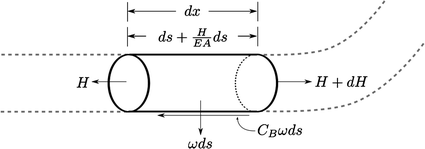
Free-body diagram for an infinitesimal cable section in contact with the seabed
Full size image

Fig. 22
Definition of geometry and parameters used in constructing a single mooring line suspended in fluid and touching a horizontal bottom boundary
Full size image
The entire cable (on the seabed and hanging in the fluid) lies in a vertical plane. Transverse seabed friction is neglected.

Figure 22 is dissected into three segments. Points a (the anchor position) and f (the fairlead position) are typically known entities based on the FOWT motions. The touch-down point B that is a parameter that is calculated in the course of iteratively solving for H and V. The displacement $ x_{0} $ identifies the transition point where $ H\left( {x_{0}^{ + } } \right) > 0 $ and $ H(x_{0}^{ - } ) = 0 $. The length of line resting on the seabed, $ L_{B} $, is a linear function proportional to the vertical force V magnitude. If the vertical force is not sufficient to suspend the cable, then $ V < \omega L $, which implies a portion of the line rests on the seabed. The difference between V and $ \omega L $ accounts for the total weight of cable resting on the seabed. This is recognised with the following expression:

$$ L_{B} = L - \frac{V}{\omega } $$

(63)

When $ L_{B} > 0 $, then Eq. (58) is violated, and the line is no longer fully suspended. Although $ L_{B} $ is useful in describing the mooring line geometry and juncture of the touch-down point, it is an essential component for determining the transition point $ x_{0} $, which is necessary to advance towards the final solution. Because the line is in static equilibrium, the horizontal forces on the line due to friction must equate to the horizontal applied force at the fairlead:

$$ H = C_{B} \omega \left( {L_{B} - x_{0} } \right) $$

(64)

With the fundamental geometric components defined, the derivation for the closed-form analytical cable model with seabed contact proceeds by defining the governing differential equations. The next step is to determine the horizontal force $ H(s) $ along the portion touching the seabed. The expression for $ H(s) $ is a prerequisite to determine the equivalent forms of Eqs. (54) and (55) for the cable/seabed contact problem.

Horizontal Force

For the case of a cable resting on the seabed, the rate of change in the element horizontal direction will be proportional to $ C_{B} \omega $. Through a summation of force in the x direction, as depicted in Fig. 21, one obtains:

$$ \begin{aligned} \sum {F_{x} } = 0 & \to H + C_{B} \omega ds = H + ds \\ & \to dH = C_{B} \omega ds \\ \end{aligned} $$

(65)

The horizontal force $ H(s) $ is found by integration Eq. (65) from a to B, Fig. 22, where the expression for the horizontal then becomes:

$$ H\left( s \right) = \left\{ {\begin{array}{*{20}l} {C_{B} \omega (s - x_{0} )} & {{\text{if }}\;\;s \le x_{0} } \\ 0 & {\text{otherwise}} \\ \end{array} } \right. $$

(66)

Given the tension component T is exclusively in the x direction at the cable/seabed interface, Fig. 22, the substitution $ T = H $ can be made in Eq. (53).

Cable Profile

The line geometry can be sought by integrating Eq. (53):

$$ \int\limits_{0}^{x(s)} {dx} = \int\limits_{0}^{s} {\left[ {1 + \frac{H(s)}{EA}} \right]ds^{{\prime }} } $$

(67)

Equation (67) leads to a series of conditional algebraic expressions based on the section of line in contact with the boundary:

$$ x\left( s \right) = \left\{ {\begin{array}{*{20}l} s & {{\text{if}}\;\;0 \le s \le x_{0} } \\ {s + \frac{{C_{B} \omega }}{2EA}\left( {s^{2} - 2x_{0} s + x_{0} \lambda } \right)} & {{\text{if}}\;\;x_{0} < s \le L_{B} } \\ {L_{B} + \frac{Hs}{EA} + \frac{{C_{B} \omega }}{2EA}\left( {x_{0} \lambda - L_{B}^{2} } \right) + \frac{H}{\omega }\sinh^{ - 1} \left[ {\frac{{\omega \left( {s - L_{B} } \right)}}{H}} \right]} & {{\text{if }}\;\;L_{B} < s \le L} \\ \end{array} } \right. $$

(68)

with $ \lambda $ equal to:

$$ \lambda = \left\{ {\begin{array}{*{20}l} {L_{B} - \frac{H}{{C_{B} \omega }}} & {{\text{if}}\;\;x_{0} > 0} \\ 0 & {\text{otherwise}} \\ \end{array} } \right. $$

(69)

The expression $ z(s) $ is found by continuing Eq. (55) beyond point B. Between the range $ 0 \le s \le L_{B} $, the vertical height is zero since the line is resting on the seabed and forces can only occur parallel to the horizontal plane. This produces:

$$ z\left( s \right) = \left\{ {\begin{array}{*{20}l} 0 & {{\text{if }}\;\;0 \le s \le L_{B} } \\ {\frac{H}{\omega }\left[ {\sqrt {1 + \left( {\frac{{\omega \left( {s - L_{B} } \right)^{2} }}{H}} \right)} - 1} \right] + \frac{{\omega \left( {s - L_{B} } \right)^{2} }}{2EA}} & {{\text{if }}\;\;L_{B} < s \le L} \\ \end{array} } \right. $$

(70)

Equations (68) and (70) produce the mooring line profile as a function of s. Ideally, a closed-form solution for l and h is sought to permit simultaneous solves for H and V, similar to Eqs. (54) and (55). This is obtained by substituting $ s = L $ into Eqs. (68) and (70) to yield:

$$ l = L_{B} + \frac{H}{\omega }\sinh^{ - 1} \left( {\frac{V}{H}} \right) + \frac{HL}{EA} + \frac{{C_{B} \omega }}{2EA}\left( {x_{0} \lambda - L_{B}^{2} } \right) $$

(71)

$$ h = \frac{H}{\omega }\left[ {\sqrt {1 + \left( {\frac{V}{H}} \right)^{2} } - 1} \right] + \frac{{V^{2} }}{2EA\omega } $$

(72)

Finally, a useful quantity that is often evaluated is the tension as a function of s along the line. This is given using:

$$ T\left( s \right) = \left\{ {\begin{array}{*{20}l} {{\text{MAX}}\left[ {H + C_{B} \omega \left( {s - L_{B} } \right) ; 0} \right]} & {{\text{if}}\;\;0 \le s \le L_{B} } \\ {\sqrt {H^{2} + \left[ {\omega \left( {s - L_{B} } \right)} \right]^{2} } } & {{\text{if }}\;\;L_{B} < s \le L} \\ \end{array} } \right. $$

(73)

3.2 Dynamic Mooring Models

The previous derivations resulted in models providing the static equilibrium forces. A different method is considered next relying on numerical integration. Convincing arguments for dynamic mooring models where provided earlier in the section through Eqs. (50) and (51); though not all dynamic cable models can capture longitudinal excitations in Eq. (50), as this depends if the model is inextensible or not (i.e. the EA cable property) (Rupe and Thresher 1975).

Choo and Casarella (1973) presented a summary of qualities various dynamic mooring models possesses, including those with inextensible elements. These early cable models were derived heuristically as a kinematic mass-spring-damper chain, akin to the system in Fig. 23 (Walton and Polachek 1960; Schram and Reyle 1968; Merchant and Kelf 1973; Ketchman and Lou 1975). The focus of this era was geared towards defining various theories and practices to simulate mooring dynamic responses. These early dynamic models lead to the progress allowing deeper waters to be reached with confidence (Skop 1988). By the late 1980s, theory fundamentals were in place. It is not coincidental that as computers became more powerful, dynamic mooring models increased in complexity, leading to rapid progress in standard design practices.

The modern era has ushered in inexpensive computational resources to render sophisticated dynamic models highly accessible features for FOWT applications. With expanded computational resources, the research envelope has shifted from developing dynamic model theories to advancing simulation features to closely replicate real-life conditions, such as contoured seabed-cable interaction, integration strategies, and fully-coupled aero-elastic-hydro-mooring dynamic analysis (Sun et al. 1994; Kamman and Huston 1999; Gobat and Grosenbaugh 2001; Gatti-Bono and Perkins 2004; Williams and Trivailo 2007; Bae et al. 2011). Dynamic mooring models can be classified into three main groups:

Lumped-mass model
Finite element model
Finite-difference model

In general, each of these models converges on nearly identical results given sufficient resolution (Ketchman and Lou 1975; Leonard and Nath 1981). The models described herein are adequate for design code checks categorised as dynamic analysis.

Fundamentals

The constituting equation describing the foundation for discretised dynamic cable models can be summarised as:

$$ {\mathbf{M}}_{i} {\ddot {\mathbf{r}}}_{i} = \sum {{\mathbf{f}}_{{i_{ext} }} } + \sum {{\mathbf{f}}_{{i_{int} }} } $$

(74)

where $ {\mathbf{M}}_{i} $ is the mass matrix, $ {\mathbf{r}}_{i} $ is the node position, and $ {\mathbf{f}}_{{i_{ext} }} $ and $ {\mathbf{f}}_{{i_{int} }} $ represent external and internal forces, respectively. This equation is provided purely for demonstration purposes of how components of the model come together, though formulations may vary depending how the theory is applied. Nodes represent $ N + 1 $ discrete points on the line, Fig. 23, where each node acceleration and velocity must be integrated to determine position. Internal forces are those defined by the element properties, and may comprise of:

Tension
Damping
Bending
Torsion

External forces are those defined by interactions with the environment, and may be comprised of:

Gravity loads from weight and buoyancy
Hydrodynamic loads
Vortex-Induced-Vibrations (VIV)
Seabed interaction
Collision with adjacent bodies

For demonstration purposes, the following vectors are defined: $ {\mathbf{t}}_{i} $ is tension, $ {\mathbf{b}}_{i} $ is structural damping, $ {\mathbf{n}}_{i} $ is the internal bending moment, $ {\mathbf{w}}_{i} $ are the gravity loads, and $ {\mathbf{h}}_{i} $ are hydrodynamic forces. Contrasting Eq. (74) to continuous models found in (Garrett 1982; Nordgren 1987):

$$ {\mu}{\ddot{\mathbf{q}}}(s,t) = \underbrace {{\left( {{\mathbf{h}} + {\mathbf{w}}} \right)}}_{{{\text{external}}\,{\text{force}}}} + \underbrace {{\left( {{\mathbf{t}} + {\mathbf{b}}} \right)}}_{{{\text{internal}}\,{\text{force}}}} $$

(75)

the resemblance is apparent. Equation (74) is the continuous interpretation of the discretised form for Eq. (75), where the units are in force-per-length. Boundary conditions are applied at the end points, nodes $ {\mathbf{r}}_{0} $ and $ {\mathbf{r}}_{N} $, which usually are not integrated since the positions are prescribed (or fixed in the case of an anchor). Although derived heuristically, this is the basis of where the three dynamic mooring model classes can trace their origins to. This fundamental representation can be expanded to include contributions from bending and torsion. Among the three dynamic models presented, the lumped-mass, finite element, and finite-difference rely on a comparable kinematic description given in Fig. 23. The size of N directly relates to the number of longitudinal and transverse vibration modes the dynamics model can capture.

Forces arising from strain, damping, gravitational loads, and hydrodynamic forces, will be the targets of this abridged presentation for the purpose of describing the lumped-mass, finite element, and finite-difference model formulations are arranged. References will be provided pointing to the relevant literature with elaborately detailed derivations. Essential differences between the three classes of dynamic mooring models are how the forces and mass matrix are discretised. Other differences among the three model classes are also described in Masciola et al. (2011).

Lumped-Mass Model

The lumped-mass model is a straightforward model to implement, making it a popular tool in the offshore community (Huang 1994; Chai et al. 2002; Buckham et al. 2004; Nicoll 2006; Williams and Trivailo 2007). Borrowing concepts from Fig. 23 and Eq. (74), the ith element is adjacent to nodes $ {\mathbf{r}}_{i - 1} $ and $ {\mathbf{r}}_{i} $, implying the element tension $ {\mathbf{t}}_{i} $ can found using:

$$ {\mathbf{t}}_{i} = k_{i}\Delta _{i} {\widehat{\mathbf{k}}}_{i} $$

(76)

where $ k_{i} = \frac{EA}{{L_{i} }} $ is the element stiffness and $ \Delta _{\text{i}} = \left\| {{\mathbf{r}}_{i - 1} - {\mathbf{r}}_{i} } \right\| $ is the stretched length. The unit vector $ {\widehat{\mathbf{k}}}_{i} = \left[ {0,0,1} \right]^{T} $ is the local element frame as depicted in Fig. 23. Equation (76) is assigned zero if $ L_{i} > \left\| {{\text{r}}_{i - 1} - {\text{r}}_{i} } \right\| $ since mooring cannot support compressive loads. Line forces are solved in a local frame fixed to the element for convenience of deriving the forcing functions, but are eventually transformed into a global orientation which the platform equation of motion is defined in. Equation (76) is an essential component of dynamic mooring models to capture dynamic tension variations, particularly those associated with Eq. (50).

The internal (structural) damping model can be incorporated based on the stretched length rate of change:

$$ {\mathbf{b}}_{i} = b_{i} {\dot{\Delta }}_{i} {\widehat{\mathbf{k}}}_{i} $$

(77)

Bending moments can be implemented on a strategy of solving the spatial derivative of a spline curve, $ {\mathbf{q}}(s) $, fitted through the node points (Buckham et al. 2004). In a three dimensional domain, the spline function at the ith element is:

$$ {\mathbf{q}}_{i} (s) = {\mathbf{A}}_{i} + {\mathbf{B}}_{i} s + {\mathbf{C}}_{i} s^{2} + {\mathbf{D}}_{i} s^{3} $$

(78)

The line/element slope arises from the spatial derivative $ \frac{{d{\mathbf{q}}_{i} }}{ds} $, the decisive ingredient for determining the bending moment:

$$ {\mathbf{n}}_{i} = \left[ {\frac{EI}{{L_{i} }}\left( {\varvec{\kappa}_{i - 1} -\varvec{\kappa}_{i} } \right)} \right] $$

(79)

with $ \varvec{\kappa}_{i} $ being a vector describing the radius of curvature derived from $ {\mathbf{q}}_{i} (s) $ in Eq. (78).

Hydrodynamic $ {\mathbf{h}}_{i} $ loads are commonly included by treating the element as a Morison element to consider the relative fluid velocity. There are various methods to derive this force (Merchant and Kelf 1973; Buckham et al. 2004; Gatti-Bono and Perkins 2004), but most approaches follow a precedent of arranging the relative fluid velocity/acceleration in components parallel and perpendicular to the element. The perpendicular relative fluid velocity/acceleration contributes quadratic drag and cross-flow added mass effects. The component parallel to the line may also provide skin friction and, in the case of chain, added mass. Directness of the lumped-mass model evolves from treating the mooring line as a discretised system as its inception. This inherently leads to a diagonal mass matrix $ {\mathbf{M}}_{i} = {\text{diag}}(m_{i} ,m_{i} ,m_{i} ) $. Other dynamic models, such as the finite element and finite-difference, proceed by discretizing the continuous partial differential equations in Eq. (75) using the method of weighted residuals or a differencing stencil to approximate gradients and time derivatives.

Consistent Finite Element Formulation

Fundamental differences between the lumped-mass model and a finite element mooring model include the following (Garrett 1982; Ran 2000):

Model initiates with the continuous model in Eq. (75).
Mass matrix discretisation: Consistent finite element model yield off-diagonal terms in $ {\mathbf{M}}_{i} $. This may couple the motion of nonadjacent nodes.
Force, boundary, and constraint discretisation.

A finite element representation for a structural cable system can be described in abridged form as (Garrett 1982; Ran 2000; Zienkiewicz and Taylor 2000):

$$ \underbrace {{\rho_{c} \int\limits_{0}^{L} {A_{j} {\ddot{\mathbf{r}}}_{i} ds} }}_{{{\mathbf{M}}_{i} }} + \underbrace {{\int\limits_{0}^{L} {\left( {EIA_{j}^{\prime \prime} {\mathbf{r}}_{i}^{\prime\prime} + \lambda A_{j}^{{\prime }} {\mathbf{r}}_{i}^{\prime } } \right)ds} }}_{{{\text{stiffness}}\,{\text{matrix}}}} = \underbrace {{\int\limits_{0}^{L} {A_{j} F_{i} ds} }}_{{{\text{external}}\,{\text{force}}}} $$

(80)

where $ A_{j} $ is the cubic interpolation (shape) function based on the node arrangement pattern on the line, and $ \lambda $ is the Lagrange multiplier to resolve the axial line tension constraint:

$$ \int\limits_{0}^{L} {P_{j} } \left[ {\left( {\frac{1}{2}{\mathbf{r}}_{i}^{{\prime }} \cdot {\mathbf{r}}_{i}^{{\prime }} - 1} \right) - \frac{\lambda }{EA}} \right]ds = 0 $$

(81)

where $ P_{j} $ is a quadratic interpolation coefficient. Both Garrett (1982) and Ran (2000) cultivate a finite element dynamic mooring model based on Eq. (75) with bending and torsion effects to result in Eqs. (80) and (81). This practice parallels Eqs. (78)/(79) for the lumped-mass model.

With the finite element model being a more rigorous formulation, it can improve the model fidelity with fewer elements compared to a lumped-mass model (Leonard and Nath 1981). This discretisation method also guarantees $ L^{2} $ stability and conservation of energy due to Galerkin orthogonality (Hughes 1977; Liu et al. 2008). The finite element model also permits external forces to be decomposed as a series of Gauss points along an element. This effectively maintains continuity and smoothness of the applied forces even if a coarse element resolution is used.

Finite-Difference Model

The finite-difference model proceeds as a Taylor series expansion of the governing partial differential equation in Eq. (74). Seminal works in this area include Van den Boom (1985) and Gobat (2000). Parallels between the finite-difference model and the method of lumped-masses is explained in Huang (1994). A distinction between finite-difference models and other dynamic mooring lines derivation is that both the time and spatial derivatives are preserved in the domain discretisation. Unlike the finite element, which computes piece-wise derivatives explicitly, the finite-difference model approximates these functions. Although the spatial and time discretisation can take many forms, one finite-difference mooring model is based on a backward difference (box) stencil and first-order Taylor expansion of Eq. (74) (Gobat 2000; Gobat and Grosenbaugh 2001):

$$ \begin{aligned} & {\mathbf{f}}_{j}^{i} + {\mathbf{f}}_{j - 1}^{i} + {\mathbf{f}}_{j}^{i - 1} + {\mathbf{f}}_{j - 1}^{i - 1} \\ & \quad = \frac{{\left( {\mu_{j}^{i} + \mu_{j}^{i - 1} } \right)\left( {{\dot{\mathbf{q}}}_{j}^{i} - {\dot{\mathbf{q}}}_{j}^{i - 1} } \right)}}{{\Delta t}} + \frac{{\left( {\mu_{j - 1}^{i} + \mu_{j - 1}^{i - 1} } \right)\left( {{\dot{\mathbf{q}}}_{j - 1}^{i} - {\dot{\mathbf{q}}}_{j - 1}^{i - 1} } \right)}}{{\Delta t}} \\ & \quad \quad \frac{{({\mathbf{t}}_{j - 1}^{i} + {\mathbf{t}}_{j}^{i} )({\mathbf{q}}_{j}^{i} - {\mathbf{q}}_{j - 1}^{i} )}}{{\Delta s}} + \frac{{\left( {{\mathbf{t}}_{j - 1}^{i - 1} + {\mathbf{t}}_{j}^{i - 1} } \right)({\mathbf{q}}_{j}^{i - 1} - {\mathbf{q}}_{j - 1}^{i - 1} )}}{{\Delta s}} \\ \end{aligned} $$

(82)

where i is the spatial derivative, j is the time variable, and f is the applied external forces. The choice of differencing stencil implicates the equation format. By incrementing the time variable forward as opposed to backward, a forward-differencing scheme is produced (Mehrabi and Tabatabai 1998). In other words, the integration strategy is central to the application of the finite-difference model. This makes it relatively straightforward to translate a mathematical model into a computer algorithm. Unlike the finite element model, the finite-difference model does not guarantee energy flux is conserved due to approximating the derivatives. As a result, stability needs can influence the number of elements, the discretisation stencil, discretisation size (both $ \Delta t $ and $ \Delta s $), and boundary condition resolution. Although this assessment also pertains to the finite element and lumped-mass models, numerical stability is less ominous with those models and can be achieved by modifying fewer parameters—such as using a coarser discretisation (i.e., increasing element size) or reducing time-step size. Finite-difference models have a proven track record providing high-fidelity modelling capabilities on par with finite element representations.

Other Caveats

Although the theory for translating a mooring system into computer code is well documented, there are several nuances with limited exposure. Tool developers new to this field commonly encounter these challenges as the model is created. The purpose here is to highlight these common challenges and provide references offering solutions to numerical instability and static convergence issues.

Numerical Stability

As with all structural models, maintaining numerical stability is essential. Instability can be controlled through adding damping, either as a structural component (Rayleigh damping) or skin drag. Cross-flow hydrodynamic damping (such as that applied using Morison’s equation) is also crucial to limit amplitude of the transverse oscillation governed by Eq. (51). Including the local line velocity in the fluid drag calculation is vital to limit transverse oscillations to within reasonable values.

Artificial numerical damping is a viable means to limit instabilities arising from high-frequency longitudinal excitations. This is introduced in few implicit numerical integration methods (Chung and Hulbert 1993). Though, when artificial damping is present, additional structural damping might not be necessary, and Eq. (77) can be omitted depending on the numerical integration strategy. There are discussions within the structural modelling community as to how reasonable and realistic damping values should be derived. There is an agreement, however, that structural damping should be sufficient to promote numerical stability, but not large enough to foster noticeable changes in the system dynamics (Balzola 1999). An additional means to promote numerical stability is by introducing bending stiffness in the model (Choo and Casarella 1973; Gobat and Grosenbaugh 2001; Buckham et al. 2004; Williams and Trivailo 2007).

Static Convergence

Numerical instability from static convergence failures is an issue many cable model developers encounter with consternation; the purpose of a dynamic mooring model is to solve the dynamic response of the line, not necessarily to solve a statics problem. But to satisfy the dynamics equation, the model must start in an equilibrium configuration to avoid excessive start-up transients. Static convergence is achieved when the $ {\ddot{\mathbf{r}}}_{i} $ term in Eq. (74) and $ {\ddot{\mathbf{q}}}_{i} $ term in Eq. (75) are zero, i.e., the no acceleration and the node forces balance. This reduces the respective equations of motion into a static equation. To the surprise of many, this can be a difficult problem to solve (De Zoysa 1978; Webster 1980; Powell and Simons 1981; Shugar 1991; Wu 1995; Zueck and Powell 1995 ; Masciola et al. 2011). Fortunately, solution strategies are numerous, and the choice of approach is a matter of preference. Note that the continuous analytical model given by Eqs. (59) and (60) do not result in a static equilibrium solution for the discretised model; though the results can be used as initial estimates to the solution. Simply solving the resulting statics equation using conventional nonlinear iterative solvers proves to be difficult due to the large condition number of the Jacobian matrix (Strang 1988). Methods to solve the discretised cable statics problem include:

Dynamic relaxation: a preliminary simulation is executed with a fixed or adaptive damping term to softly arrive at the statics solution (Webster 1980; Shugar 1991; Wu 1995).
Shooting method: the method relies on iterating boundary conditions until a targeted solution is achieved (De Zoysa 1978; Friswell 1995; Masciola et al. 2011).
Modified root-finding methods: the step size advancing the solved variable is reduced based on iteration history to avoid exceeding the radius of convergence (Powell and Simons 1981; Zueck and Powell 1995).

4 Structural Design

Erin E Bachynski

Various types of structural analysis may be performed in order to assess the safety of a FOWT design with respect to the fatigue limit state (FLS), ultimate limit state (ULS), and accidental limit state (ALS) which are described in standards such as DNV-OS-J103 (2013). A typical design process includes a progression from simplified frequency-domain models, to global models which can capture some cross-sectional loads, to detailed local models for evaluation of stress concentration factors and local strength. The simple frequency-domain models are used to obtain first estimates of the motions in waves, which can then be used in preliminary mooring system design. More detailed global analysis models include more interaction between the structure, waves, wind, wind turbine control system, as well as accounting for flexibility in selected components. Such global analysis models must be accurate enough to capture important effects, but also computationally efficient in order to be able to simulate a wide range of design load cases within a reasonable amount of time.

Global analysis models are used to provide information about the overall structural strength and system behaviour as well as to provide input for local analysis models. The structure is subjected to static loads (gravity, buoyancy, and hydrostatic pressure) as well as dynamic loads from the environment, inertia, and operation. In general, time-varying loads will give time-dependent responses (displacements, strains, stresses). For loading of frequency less than about 1/4 of the lowest structural natural frequency, quasi-static analysis may be appropriate. In the case of floating wind turbines, the range of excitation frequencies generally includes frequencies well above this lower limit, such that dynamic analysis is needed. Dynamic response may be greater or less than the corresponding static response.

Global analysis models using beam or shell elements may not, however, be able to capture stress concentration factors in welded joints or scantlings, or to verify local pressure loads. Local final element analysis (FEA) using solid elements may therefore be needed. The boundary conditions for local FEA may be obtained from the global analysis model and applied in a more detailed model.

For any type of numerical structural analysis, the key is physical and theoretical understanding of the mathematical model as well as its limits. It is therefore recommended to start with relatively small and simple models, and then refine as needed. One should also take care to use reliable, well-understood finite elements, and to check that the solution has converged before examining the results.

4.1 Linear Rigid Body Dynamics

The simplest dynamic structural model of a FOWT is a single rigid body. One can define up to six traditional global motions about a given inertial reference point: surge $ \zeta_{1} $, sway $ \zeta_{2} $, heave $ \zeta_{3} $, roll $ \zeta_{4} $, pitch $ \zeta_{5} $, and yaw $ \zeta_{6} $. These global motions can be represented mathematically by the motion vector, $ \vec{\zeta } $, where

$$ \vec{\zeta } = \left[ {\zeta_{1} (t),\zeta_{2} (t),\zeta_{3} (t),\zeta_{4} (t),\zeta_{5} (t),\zeta_{6} (t)} \right]^{T} $$

(83)

and t represents time. Newton’s second law is then applied in an inertial reference frame as:

$$ {\mathbf{M}}\vec{\ddot{\zeta }} = \vec{F} $$

(84)

where M is a 6 × 6 matrix containing the entries $ {\mathbf{M}}_{{{\mathbf{ij}}}} $ representing the dry mass of the structure, with the inertia computed about the body reference point; $ \vec{F} $ is a time-dependent vector of all of the forces acting on the body; and the double dot represents two differentiations with respect to time.

For a moored floating body subjected to waves, a linear analysis of the global motions can be carried out by separating the force vector into several components: an added mass component which opposes the body acceleration, a linear damping component which is proportional to the body velocity, a linear stiffness due to hydrostatics which is proportional to the body motion, a linear stiffness due to the mooring system, and external wave excitation loads. By collecting the added mass, damping, and stiffness terms on the left hand side, the equation of motion becomes:

$$ \left[ {{\mathbf{M}} + {\mathbf{A}}} \right]\vec{\ddot{\zeta }} + {\mathbf{B}}\vec{\dot{\zeta }} + \left[ {{\mathbf{C}} + {\mathbf{K}}} \right]\vec{\zeta } = \vec{X} $$

(85)

where A represents added mass coefficients, B represents damping coefficients, and C and K represent linear stiffness coefficients due to hydrostatics and the mooring system, respectively. A, B, C, and K are 6 × 6 matrices, including coupling terms, and A and B are generally frequency-dependent. The 6 × 1 frequency- and amplitude-dependent vector $ \vec{X} $ contains the external wave excitation force for each mode of motion.

For a linear wave-only analysis of a floating body, it is then convenient to consider the problem in the frequency domain (Faltinsen 1990). For a floating offshore wind turbine, such an approach can be extended with linearised approximations of the aerodynamic loads ( Bachynski 2014; Kvittem 2014). In order to include nonlinear load effects in a rigid body model, the equations of motion should, however, be solved in the time domain. In that case, the frequency-dependence can be included through a convolution integral or by a state-space representation of the time-dependent coefficients (Taghipour et al. 2008). A rigid body model does not provide sufficient information for structural strength analysis, and one must therefore examine alternative methods.

4.2 Finite Element Methods

Rather than limiting the analysis to six rigid body motions, the structure may be discretised using a number of finite elements. These elements have approximate representations of the mass and stiffness properties of the structure. By combining the mass, damping, and stiffness matrices corresponding to all of the degrees of freedom of many individual elements in a consistent manner, the static and dynamic structural responses of a physical structure can be estimated. Finite element analysis (FEA) provides a piecewise approximation of field quantities such as stress and strain.

Beam elements can capture the overall behaviour of long, slender structures. Shell elements, which remove a level of abstraction from the beam element model, can capture flexural stresses which are not considered in a beam model. A solid element model removes another level of abstraction, but requires even greater computational effort.

In FEA, regardless of the element type, the governing equation for structural dynamics can be formulated by requiring that the virtual work done by externally applied loads be equal to the sum of the virtual work absorbed by inertial, dissipative, and internal forces. The global form of the governing equation can be written as in Eq. (86), assuming that the element mass ($ {\mathbf{M}}_{{\mathbf{g}}} $) and damping ($ {\mathbf{B}}_{{\mathbf{g}}} $) matrices follow from the discretisation and use the same shape function as the stiffness matrix.

$$ {\mathbf{M}}_{{\mathbf{g}}} \vec{\ddot D} + {\mathbf{B}}_{{\mathbf{g}}} \vec{\dot{D}} + \vec{R}^{\text{int}} = \vec{R}^{ext} $$

(86)

In Eq. (86), $ \vec{D} $ is the system displacement vector, $ \vec{R}^{\text{int}} $ are the internal reaction forces and $ \vec{R}^{ext} $ are the external loads. For a linear elastic material, the internal forces can be written:

$$ \vec{R}^{\text{int}} = {\mathbf{K}}_{{\mathbf{g}}} \vec{D}. $$

(87)

In practice, however, the stiffness matrix is not necessarily linear: $ {\mathbf{K}}_{{\mathbf{g}}} $ is, in general, a function of $ \vec{D} $. For FOWTs, nonlinearities in the physical problem can be related to geometrical nonlinearities (such as the large deflections of the blades or mooring lines), nonlinear force boundary conditions (such as the generator torque which is applied by the turbine controller), displacement boundary condition nonlinearity (such as contact), or in some cases by material nonlinearities.

Equation (86) is a system of coupled second-order differential equations that are continuous in time (and discretised in space). The formulation of the mass, damping, and stiffness matrices, as well as the load and displacement vectors depends on the type of elements to be used. A brief review of classical and Timoshenko beam theories, and the formulation of beam element stiffness, mass, and damping matrices is given here. Traditional structural mechanics (Hibbeler 2011) and finite element textbooks (Cook et al. 2002) should be consulted for greater detail.

Beam Theory

Classical beam theory, also known as Euler-Bernoulli beam theory, is a mathematical description of the relationship between the applied load and the deflection of a slender beam. The theory is applicable for long slender beams and relatively small deflections. The shear deformation is assumed to be much smaller than the transverse deformation. Consider the beam in Fig. 24, which has its long axis along the x-axis and deflects in the y-direction, and the corresponding cross section in Fig. 25.

From the mechanics of materials, the time-varying bending moment sustained by the beam $ M(x,t) $ is related to the bending deformation $ w(x,t) $ as in Eq. (88), where E is the Young’s modulus, and I is the cross-sectional area moment of inertia about the z axis.

$$ M(x,t) = EI(x)\frac{{\partial^{2} w(x,t)}}{{\partial x^{2} }} $$

(88)

By considering the summation of forces (Eq. 89) and of moments (Eq. 90) on an infinitesimal element (Fig. 25), the shear force V is found to be related to the moment as in Eq. (91) for Euler-Bernoulli beams. The cross sectional area is denoted A and the total external force per unit length is f. In Eq. (90), the rotational inertia of the infinitesimal element is assumed to be very small, which results in the right hand side of the equation being zero. In order to obtain Eq. (91), terms with $ (dx)^{2} $ are neglected, as these are much smaller than the terms which are proportional to dx.

$$ \left( {V(x,t) + \frac{\partial V(x,t)}{\partial x}dx} \right) - V(x,t) + f(x,t)dx = \rho A(x)dx\frac{{\partial^{2} w(x,t)}}{{\partial t^{2} }} $$

(89)

$$ \begin{aligned} & \left[ {M(x,t) + \frac{\partial M(x,t)}{\partial x}dx} \right] - M(x,t) \\ & \quad + \left[ {V(x,t) + \frac{\partial V(x,t)}{\partial x}dx} \right]dx + \left[ {f(x,t)dx} \right]\frac{dx}{2} = 0 \\ \end{aligned} $$

(90)

$$ V(x,t) = - \frac{\partial M(x,t)}{\partial x} $$

(91)

Equation (92) gives the final dynamic Euler-Bernoulli beam equation, obtained by substituting Eq. (88) into Eq. (91).

$$ \rho A(x)\frac{{\partial^{2} w(x,t)}}{{\partial t^{2} }} + \frac{{\partial^{2} }}{{\partial x^{2} }}\left[ {EI(x)\frac{{\partial^{2} w(x,t)}}{{\partial x^{2} }}} \right] = f(x,t) $$

(92)

The Euler-Bernoulli formulation is a special case of Timoshenko beam theory. Timoshenko beam elements account for the deformation due to shear and are appropriate for thicker beams. The corresponding relationship between the shear and moment for a Timoshenko beam is given in Eq. (93).

$$ V(x,t) = \kappa^{2} AG\left[ {\psi (x,t) - \frac{dw(x,t)}{dx}} \right] $$

(93)

In Eq. (93), $ \kappa^{2} $ is a dimensionless shear coefficient which depends on the shape of the cross section, and G is the shear modulus. The deformation denoted $ \psi (x,t) $ includes the effects of bending and shear deformation. The resulting coupled dynamic beam equations for a Timoshenko beam, including rotational inertia, are given in Eqs. (94) and (95). Note that, for the sake of space, the dependence on $ x $ and $ t $ is not shown explicitly in Eqs. (94) and (95).

$$ \frac{\partial }{\partial x}\left[ {EI\frac{\partial \psi }{\partial x}} \right] + \kappa^{2} AG\left( {\frac{\partial w}{\partial x} - \psi } \right) = \rho I\frac{{\partial^{2} \psi }}{{\partial t^{2} }} $$

(94)

$$ \frac{\partial }{\partial x}\left[ {\kappa^{2} AG\left( {\frac{\partial w}{\partial x} - \psi } \right)} \right] + f = \rho A\frac{{\partial^{2} w}}{{\partial t^{2} }} $$

(95)

Stiffness Matrix for Beam Elements

In order to apply the beam theory in the finite element formulation, one must develop the formulation for a beam element. The formulation of the mass and stiffness matrix for beam elements can be illustrated by examining a two-dimensional beam along the x-axis, disregarding the axial degrees of freedom. This simple beam, shown in Fig. 26, therefore has two nodes, and each node has two degrees of freedom: lateral translation $ v $ and rotation $ \theta $.

The stiffness matrix for our simple beam can be obtained by applied a unit deformation in each degree of freedom—one by one—and computing the resulting internal forces in the element in order to achieve force and moment balance. For example, if one applies a unit deformation $ \upsilon_{1} = 1 $ and zero deformations in the other degrees of freedom, the beam now takes the form of Fig. 27.

By considering the element as cantilevered at node 2 and loaded by the force $ k_{11} $ and moment $ k_{21} $ at node 1, in order to obtain the desired deflections, one finds:

$$ \frac{{k_{11} L^{3} }}{3EI} - \frac{{k_{21} L^{2} }}{2EI} = 1 $$

(96)

$$ \frac{{k_{21} L}}{EI} - \frac{{k_{11} L^{2} }}{2EI} = 0 $$

(97)

By solving the set of Eqs. (96) and (97) and requiring force and moment equilibrium, the resulting components of the first column of the element stiffness matrix become $ k_{11} = \frac{12EI}{{L^{3} }} $, $ k_{21} = \frac{6EI}{{L^{2} }} $, $ k_{31} = - \frac{12EI}{{L^{3} }} $, $ k_{41} = \frac{6EI}{{L^{2} }} $. A similar approach can be used to obtain the full stiffness matrix for this simple example.

For more general beam elements, additional degrees of freedom should be considered. Often, 12 degrees of freedom (6 at each node) are included for beams, and either Euler-Bernoulli or Timoshenko beam theories are used in the development of the stiffness matrix. Furthermore, for more general elements, the stiffness matrix is established based on stress-strain relations, strain-displacement relations, and energy considerations.

An important concept in the more general formulation of the stiffness matrix is the shape function. In order to provide a representation of a continuous function over an element, a polynomial shape function provides a basis for interpolation which is continues and differentiable. For beam elements, a cubic curve is a typical basis for the shape function.

Mass Matrix

There are several ways to formulate the mass matrix for FEA: lumped, consistent, combined, HRZ lumping, or optimal lumping (Cook et al. 2002). A lumped mass model, which places particle masses at nodes, yields a diagonal mass matrix, which is convenient for explicit time domain integration. A consistent mass matrix uses the same shape function as the stiffness matrix. For implicit time domain integration, commonly employed for dynamic analysis of FOWTs, it is less important to obtain a diagonal mass matrix, as non-diagonal terms in the stiffness matrix are also present on the left hand side of the equation. Therefore, it is typical to describe the mass of a beam element using cubic shape functions.

Structural Damping

The damping term in Eq. (86) accounts for the dissipation of energy, which is important for limiting the structural response. Real sources of damping include viscous damping (proportional to velocity), hysteresis damping in the material, Coulomb damping (dry friction), and radiation damping (the generation of waves in another medium such as soil or water). In a FOWT analysis, the hydrodynamic viscous and radiation damping may be accounted for in the damping or excitation loads, but one often also models the remaining “structural” damping through a small viscous term. Rayleigh damping is a convenient formulation for the structural damping in finite element analysis. The structural damping $ {\mathbf{B}}_{{{\mathbf{Rayleigh}}}} $ can be specified as a linear combination of the mass and stiffness matrices, as in Eq. (98). (More precisely, the tangential damping matrix is a function of the tangential mass and stiffness matrices.) In Eq. (98), $ a_{1} $ is the mass-proportional coefficient, and $ a_{2} $ is the stiffness proportional coefficient.

$$ {\mathbf{B}}_{{{\mathbf{Rayleigh}}}} = a_{1} {\mathbf{M}}_{{\mathbf{g}}} + a_{2} {\mathbf{K}}_{{\mathbf{g}}} $$

(98)

If global coefficients $ a_{1} $ and $ a_{2} $ are used, the Rayleigh damping formulation gives an orthogonal structural damping matrix. Mass-proportional damping is effective for low frequencies, while stiffness-proportional damping is effective for high frequencies. For a floating system, which may have important rigid-body motions, it is typical to set $ a_{1} = 0 $. The damping ratio then becomes a linear function of frequency.

4.3 Modal Methods

As an alternative to finite element methods, modal methods use a reduced number of degrees of freedom. That is, certain structural deformation patterns are defined, and the time-varying structural deformations are found from the sum of a combination of these patterns (or mode shapes). If the mode shapes are determined accurately, modal analysis is reasonably accurate and computationally efficient for wind turbine analysis. The well-known FAST software from NREL is based on a combination of modal and multibody dynamics formulations. Nonlinearity on the load side of the equation can be accounted for, though material nonlinearity (elasto-plastic behaviour) and geometrical stiffening due to large deformations cannot be considered. The key advantage to such analysis is its computational efficiency. An important disadvantage of modal analysis is that it requires accurate pre-processing of the system modes, and can only capture the modes which are identified and included.

An example of modal decomposition is shown in Fig. 28. The fore-aft (FA) tower modes are shown for different frequencies for two different platforms. These modes include the low-frequency surge mode, as well as a mode which is considered platform pitch for the spar and includes bending for the TLP. Although some of the mode shapes are similar, there are differences in the frequencies: even though the tower structure is identical, the base support has a significant effect. In a modal analysis, the displacement of the tower would be computed as a superposition of these modes combined with several side-side and twist modes, such that the tower could easily be modelled with very few degrees of freedom. It is important to note that these frequencies and mode shapes are dependent on the substructure which supports the tower and must be recomputed for a new substructure.

The mass, stiffness, and damping matrices for modal decomposition are formulated slightly differently than in a pure finite element formulation, but the same principles for global analysis apply.

4.4 Global Analysis Procedure

Static Equilibrium

Before carrying out any dynamic analyses of a FOWT, one must first determine the deformations and stresses in the structure under gravity, buoyancy, and other constant loads. For a FOWT, the constant loads might include current-induced drag, mean wave drift forces, or mean thrust at a given mean wind speed.

A static equilibrium calculation may be performed by incrementally increasing the applied loads from zero up to their nominal value. During each incremental step, an iterative procedure, such as Newton-Raphson, may be applied. The Newton-Raphson algorithm uses predictor-corrector steps: the displacement under the new loads is computed based on the present tangential stiffness matrix, convergence is checked, and one computes a new tangential stiffness matrix and displacement if convergence criteria are not met. Figure 29 shows the results of a static equilibrium calculation of a spar FOWT.

Decay and Eigenvalue Analysis

After the mathematical model of the FOWT structure is established and static equilibrium achieved, determining the natural frequencies of the system is an important step.

If the rigid body motions are of primary interest, a decay analysis may be used to establish the damped natural frequencies. In a decay analysis, the structure is displaced in one of the rigid body motions and then allowed to freely return to its equilibrium position. The resulting time series of the displacement can be analysed to determine the damped natural frequencies and the linear and quadratic damping in the model (Hoff 2001).

For flexible structures, however, a more complete eigenvalue analysis may be needed in order to determine the natural frequencies including structural deformations. Some important frequencies in the structural model include the first and second tower bending modes, the collective and individual blade modes, flexural modes within the hull, and for tension leg platform FOWTs, the tendon transverse and axial frequencies.

An eigenvalue analysis is performed by identifying the solutions to the homogeneous, undamped, linearised form of Eq. (86):

$$ {\mathbf{M}}_{{\mathbf{g}}} \vec{\ddot D} + {\mathbf{K}}_{{\mathbf{g}}} \vec{D} = \vec{0} $$

(99)

for harmonic displacements, $ \vec{D} = \vec{\bar{D}}\sin \left( {\omega t} \right) $. The eigenvector problem then becomes:

$$ \left[ {{\mathbf{K}}_{{\mathbf{g}}} - \omega^{2} {\mathbf{M}}_{{\mathbf{g}}} } \right]\vec{\bar{D}} = 0 $$

(100)

Equation (100) may be solved for nonzero displacement vectors ($ \vec{\bar{D}} $, the eigenmodes of the structure) in combination with particular frequencies ($ \omega $, the eigenfrequencies). If these modes are lightly damped, any excitation at the eigenfrequencies can result in significant and potentially damaging responses. For FOWTs, an important consideration is the interaction between the tower bending frequency and the blade passing (3p) frequency: the tower bending frequency on a floating platform differs from that of the same tower on a different platform or on land due to the change in the boundary conditions. As such, designers must exercise caution to avoid any potential operations during which the blades provide excitation at the tower natural frequency for the particular platform. This problem may be avoided by modifying the stiffness or mass of the tower and rotor, or by modifying the operation of the turbine.

Time Domain Response Analysis

The majority of the analyses carried out for checking the structural strength of a FOWT are dynamic analyses. That is, the governing FE equations (Eq. 86) are solved step-by-step in time: the response is computed at discrete time instants ($ t =\Delta t,2\Delta t, \ldots ,n\Delta t $).

In general, explicit or implicit methods can be used for time integration. An explicit method relies only on historical data to compute the response $ \vec{D}_{n + 1} $, while an implicit method contains the terms $ \vec{\dot{D}}_{n + 1} $ and $ \vec{\ddot D}_{n + 1} $ on the right hand side of the equation. Explicit algorithms require a smaller time increment $ \Delta t $ for stability, but the computation for each time step is more efficient. Implicit algorithms require more computational time per step, but fewer total steps (Cook et al. 2002). Furthermore, implicit algorithms are better suited to structural dynamics problems, such as the analysis of FOWTs.

A commonly used family of implicit algorithms is the Newmark-Beta family. The Newmark relations are:

$$ \vec{\dot{D}}_{n + 1} = \vec{\dot{D}}_{n} +\Delta t\left[ {\gamma \vec{\ddot D}_{n + 1} + \left( {1 - \gamma } \right)\vec{\ddot D}_{n} } \right] $$

(101)

$$ \vec{D}_{n + 1} = \vec{D}_{n} +\Delta t\vec{\dot{D}}_{n} + \frac{1}{2}\Delta t^{2} \left[ {2\beta \vec{\ddot D}_{n + 1} + (1-2\beta )\vec{\ddot D}_{n} } \right] $$

(102)

where $ \gamma $ and $ \beta $ are numerical factors which control the accuracy, numerical stability, and the amount of algorithmic (numerical) damping (Cook et al. 2002). By applying the Newmark relations to Eq. (86) and eliminating terms including $ \vec{\ddot D}_{n + 1} $ and $ \vec{\dot{D}}_{n + 1} $, one obtains:

$$ \begin{aligned} {\mathbf{K}}^{{{\mathbf{eff}}}} \vec{D}_{n + t} & = \vec{R}_{n + 1}^{ext} + {\mathbf{M}}_{{\mathbf{g}}} \left[ {\frac{1}{{\beta\Delta t^{2} }}\vec{D}_{n} + \frac{1}{{\beta\Delta t}}\vec{\dot{D}}_{n} + \quad \left( {\frac{1}{2\beta } - 1} \right)\vec{\ddot D}_{n} } \right] \\ & \quad + {\mathbf{B}}_{{\mathbf{g}}} \left[ {\frac{\gamma }{{\beta\Delta t}}\vec{D}_{n} + \left( {\frac{\gamma }{\beta } - 1} \right)\vec{\dot{D}}_{n} +\Delta t\left( {\frac{\gamma }{2\beta } - 1} \right)\vec{\ddot D}_{n} } \right]. \\ \end{aligned} $$

(103)

The Newmark-Beta algorithm of Eq. ( 103) is unconditionally stable for $ 2\beta \ge \gamma \ge 0.5 $. Algorithmic damping is introduced for $ \gamma > 0.5 $, but the accuracy is then reduced from $ O(\Delta t^{2} ) $ to $ O(\Delta t) $. Algorithmic damping is desirable for dissipating energy in high-frequency components of the response that are related to discretisation, but undesirable for the frequencies of interest (Krenk 2009).

For a linear stiffness matrix $ {\mathbf{K}}_{{\mathbf{g}}} $, the effective stiffness matrix ($ {\mathbf{K}}^{{{\mathbf{eff}}}} $) is given by Eq. (104).

$$ {\mathbf{K}}^{{{\mathbf{eff}}}} = \frac{1}{{\beta\Delta t^{2} }}{\mathbf{M}}_{{\mathbf{g}}} + \frac{\beta }{{\gamma\Delta t}}{\mathbf{B}}_{{\mathbf{g}}} + {\mathbf{K}}_{{\mathbf{g}}} $$

(104)

In order to account for geometric nonlinearities, $ {\mathbf{K}}_{{\mathbf{g}}} $ may be replaced by the tangential stiffness matrix and a Newton-Raphson iteration procedure may be used. As in the static equilibrium calculation, the displacements are computed iteratively during each time step, and the tangential stiffness matrix is updated.

Example: Beam Element Model of a Tension Leg Platform Wind Turbine

Consider the tension leg platform (TLP) FOWT designs in Fig. 30. In order to determine which (if any) of these designs is feasible, how should one carry out an efficient initial screening of the static, extreme, and fatigue loads in the tower and tendons?

A common error in this type of analysis is to begin by building a complete model and simply running a computer program. The first step in global analysis should be a simple preliminary analysis which gives insight into the expected results. For TLP FOWTs, a spreadsheet analysis is useful for estimating the natural periods and mean offset. Frequency-domain rigid body analysis can be used to quickly estimate the standard deviations of the motions and tendon tension in many sea states ( Bachynski 2014).

After conducting the preliminary simplified analyses and eliminating any problematic designs, one may begin to carefully construct a global analysis model.

One of the first choices that the analyst must make is the element type to be used in the model. In the stated problem description, the tendons and tower are of interest, so it is logical to choose flexible elements for those components. Beam elements are an appropriate choice, since the tower and tendons are long and slender. The blades are even more flexible than the tower and tendons, so it would be reasonable to model them with flexible beam elements as well. On the other hand, the hull itself is likely to be stiffer than the tower and tendons, so one may consider using a rigid body in order to improve the speed of the simulation. In that case, however, the connection between the hull and tower in the global model should be carefully considered in order to avoid a sudden change of stiffness at the point of interest.

The boundary conditions in the model are another important consideration. If the FOWT is anchored to the seabed, what are the boundary conditions at the anchors? How are different elements in the FEA connected to each other? For anchors (or piles), the connection at the seabed depends on the physical conditions. Pinned connections, which allow rotation but not translation, may be appropriate for the tendons if the connection to the soil can be considered relatively rigid. Springs and friction models to represent soil behaviour may be needed for other models. The connection between the tower and the hull may similarly require thought in order to appropriately model the physical structure.

Once the elements of the model are set, the first calculation is to obtain static equilibrium. The analyst should not only verify that the still water position of the structure matches his or her expectations, but also that the solution has converged numerically within the chosen tolerances and that the loads in the different components are sensible and in agreement with each other. For the TLP FOWT example, it is especially important to check that the compression in the base of the tower matches the expected weight that should be carried and that the tendon tension values are correct at both the fairlead and the seabed. The output of the computer program should also be understood in light of the finite element model: there may be differences in the reported internal forces and moments based on the shape factors used for the mass distribution.

Before carrying out dynamic analyses in wind and waves, it is also expected that the analyst will carefully check the model. Important types of analysis for checking the model include eigenvalue calculation, decay tests, wave-only tests, and wind-only tests. In addition to these checks, one should ensure that the time-stepping parameters are appropriate: the numerical solution should converge at each time step, the results should not change when the time step is reduced, and the amount of numerical damping in the numerical algorithm should be known and understood. The size of the elements should also be investigated. In general, it is recommended to avoid sudden changes in element size, and the element size should be appropriate for the type of element and loading.

After the model has been checked, the analyst will likely perform extensive dynamic analysis. The results of such analyses should be carefully investigated and checked. During the results check, one must also account for the limitations of the numerical model. For example, buckling loads and the limits of linear material behaviour may occur without the computer program identifying these events. It is the analyst’s responsibility to critically examine the results. The limits of the numerical model may also include the load models themselves: for the TLP FOWTs shown above, ringing loads may be critical, but a hydrodynamic load model for ringing may not be present in all software (Bachynski and Moan 2014).

4.5 Local Finite Element Analysis

Structural failure often occurs due to local stress raisers (welds, doorways, connections). The details of such stress raisers cannot generally be captured in the global finite element analysis. In some cases, a stress concentration factor (SCF) for a given design detail may be tabulated in standards such as DNV-RP-C203, such that the calculated stress in the global model can be related to the local stress. In other cases, the stress concentration factor may be unavailable, or one may simply desire a better understanding of the stress distribution in the material. In those cases, a detailed local finite element analysis may be carried out.

A local FEA may be carried out with boundary conditions provided by the global FEA, or with unit loading in different directions in order to calibrate SCFs for fatigue design. For FOWTs, typical details for local analysis include connections between bracings and columns on semi-submersibles, joints in TLP concepts, fairlead attachment points, and ladders and doors. The extent of the local model should be chosen such that effects due to the boundaries are sufficiently small. An example of stress calculation for a brace-to-column connection is shown in Fig. 31.

If the local analysis is carried out based on the boundary conditions from the global analysis model, it is important to keep in mind that the global analysis is unaffected by the local analysis. That is, one should check that the global analysis mesh is sufficiently refined and that the stresses along the cut match between the two analyses. A common problem is that the global mesh is effectively too stiff near joints and cuts, which may lead to underestimation of the local stress.

If the hot spot stress is to be computed using a refined local mesh with unit loading, several different types of elements may be used. For plated structures, thick plate and shell elements (arranged in the mid-plane of the structural components) may be appropriate. 8-noded hot spot shell elements give reliable hot spot stresses at points 0.5t and 1.5t from the intersection of interest (where t is the thickness) and the stress concentration may be interpolated using an appropriate curve (DNV-RP-C203 2010).

Three-dimensional solid elements are another option, and are well-suited for complex structures. The number of elements required to capture the stress distribution depends on the type of element. For 20-node hexahedral elements, one element over the thickness may be sufficient to capture a linear stress distribution, while four times as many 8-node elements could be required. In the solid element model, the fillet weld will likely be included, which will naturally limit the size of the mesh.

Local finite element analysis is also important for checking the detailed design of plates and stiffeners. Pressure loads (hydrostatic and hydrodynamic) are important for determining initial plate thicknesses and stiffener arrangements for FOWT hulls, while loads due to ship collisions or ice typically require additional local analysis.

5 Review of Numerical Modelling Design Codes

Mairéad Atcheson

The design of FOWTs is a relatively new topic, with only a few prototype FOWT devices deployed in recent years. In order to progress the development of the FOWT industry it is necessary create numerical modelling tools to inform the design process and predict the structural integrity of devices, ensuring the survivability and performance of a device once deployed. A key objective of a FOWT model is to find the net force of a fluid(s) on a structure, to inform the design loads required for structural analysis and detailed design stages (see Sect. 1 of Chapter “Key Design Considerations”).

Numerical modelling simulations can be carried out in the time or frequency domain. The decision on which method to use depends on the required model outputs, as method has advantages and limitations. Initial FOWT studies carried out in the frequency domain proved useful in the demonstration of the technical feasibility of FOWTs. However, frequency-domain models are not capable of capturing the nonlinear dynamic characteristics or transient loading events which are important to the dynamic response of FOWTs. Matha et al. (2009) showed that the use of a frequency domain model may lead to natural frequencies being wrongly predicted because some couplings between the platform motion and the flexible tower and blades were not accounted for these results highlighted the necessity of undertaking FOWT calculations in the time domain. Numerous time domain numerical analysis codes have been developed to simulate the aero-hydro-servo-elastic response of FOWTs, and an overview of many of these design tools is presented in Cordle and Jonkman (2011).

Section 5.1 will provide an overview of some of the design codes currently available for FOWT applications. A number of code comparison studies have also been completed to compare the different codes under development and are presented in Sect. 5.2.

5.1 Floating Offshore Wind Design Codes

Several simulation codes capable of modelling FOWTs are presently under development by FOWT device developers, commercial consultancy companies and research institutes. In general, code developers have approached the task in two manners. Many of the codes were originally developed for the design of onshore wind turbine devices and additional modules have been added to these codes to model floating platforms and mooring systems. Others have approached the task with a code capable of modelling floating platforms, and in this case the developers have included additional modules to represent the wind turbine, including the aerodynamics loading on the support structure and a control module for the turbine.

Design tools capable of modelling FOWTs currently available include (but are not limited to): FAST, SIMPACK, Bladed, SIMA workbench and HAWC2. Table 3 provides an overview of the existing modelling capabilities used by each code to model the structural dynamics, aerodynamics, hydrodynamics and mooring system. For a more complete list of simulation tools used to model FOWTs see Robertson et al. (2014a, b).

Table 3 Summary table of numerical modelling code capabilities (adapted from Robertson et al. 2014a, b)

Full size table

A brief description of the different design codes listed in Table 3 are presented in the following section. The description includes some background information on the codes and describes the methods applied to simulate the aerodynamics, hydrodynamics, mooring lines and structural dynamics for FOWTs. The information on the individual code capabilities is based on the most recent version of the code available at the time of writing, however it should be noted that most numerical modelling codes are continuously being developed to expand their capabilities.

FAST (Fatigue, Aerodynamics, Structures and Turbulence) (NREL)

FAST is an open-source design tool capable of modelling the dynamic response of two- and three-bladed horizontal axis wind turbines. It was originally developed by National Renewable Energy Laboratory (NREL) and Oregon State University, but post 1996 further code development has been completed by NREL alone. FAST was originally developed for predicting loads on land-based and offshore bottom-mounted wind turbines, but the code capabilities were extended with additional modules added to permit the modelling of FOWTs. The code comprises of modules representing different aspects of a FOWT to enable coupled nonlinear aero-hydro-servo-elastic analysis in the time domain. Further development of FAST code continues at NREL, with the introduction of a new modularisation framework in FAST v8 (Jonkman 2013). The new modularisation framework supports module-independent inputs and aims to improve numerical performance and robustness, as well as increasing module sharing and code development within the wind energy community. Various modules of FAST have also been coupled with other dynamic analysis programs to model the dynamics of FOWTs (i.e. Simo, Riflex and AeroDyn as presented in Robertson et al. 2014a, b).

FAST v8 incorporates major changes from the previous versions with several new capabilities introduced, most significantly the ability to incorporate new functionalities in the form of modules (Jonkman and Jonkman 2015). All of the modules are open source and available on the NREL website. Figure 32 illustrates the core modules of FASTv8 for floating wind turbine systems.

The wind turbine aerodynamics module (AeroDyn) uses a quasi-static blade element/momentum (BEM) theory with dynamic stall and an optional dynamic inflow theory. The latest version of the code released by NREL is AeroDyn v.15, the source code for version 15 was entirely rewritten to be fully compatible with the FAST modularisation framework (Jonkman et al. 2015a).

Improvements made for the modelling of FOWTs include changes to the hydrodynamic load calculations algorithms in HydroDyn. HydroDyn is a time domain hydrodynamics module. It is capable of modelling the hydrodynamic loading on multi-member structures and can be coupled to FAST v8 or driven as a standalone code. HydroDyn can simulate regular or irregular waves and currents and solves for the hydrostatic, radiation, diffraction and viscous loads on the wind turbine platform. Multiple approaches to calculate the hydrodynamic loads on a structure can be applied in HydroDyn, including potential flow theory, strip theory or a hybrid combination of the two. HydroDyn can describe the wave climate using first-order and second-order wave theory, with the option to include directional spreading (Jonkman et al. 2015b).

Different mooring modules are available for use with FAST v8, including a quasi-static mooring line model MoorDyn (Hall 2015) and FEAMooring (Bae 2014) a finite-element based mooring dynamics module. The structural dynamics are simulated using the ElastoDyn module and the control and electrical system can be modelled in the ServoDyn module.

SIMPACK (SIMPACK AG)

SIMPACK is a general purpose multibody system (MBS) code developed by SIMPACK AG, which is used by the automotive, railway, aerospace and robotics industries. SIMPACK Wind provides an extension to the code that allows integrated wind turbine modelling. An interface between the Energy Research Centre of the Netherlands’ (ECN) Aero-Module and SIMPACK has also been developed (Bulk 2012). The ECN Aero-Module is a BEM code with advanced correction models and is based on the BEM implementation in PHATAS (Lindenburg and Schepers 2000).

Researchers at Stuttgart’s Chair of Wind Energy (SWE) at the University of Stuttgart added an extension to the SIMPACK code to simulate FOWTs. In order to support the simulation of FOWTs in SIMPACK, two hydrodynamic modelling methodologies developed by SWE (SIMorison and SIMHydro Force Elements) were implemented. The SIMHydro module couples HydroDyn to SIMPACK ( Matha and Beyer 2013). In order to enable coupling of the codes, the original input file for HydroDyn is modified allowing users to select between the SIMorison and linear hydrodynamics module, and to define the properties of the mooring system.

For mooring systems, SIMorison may be used to model the hydrodynamic loads on mooring lines of FOWTs. The original HydroDyn quasi-static mooring line module is replaced by an MBS-mooring-line model where each line is discretised into separate rigid or flexible bodies connected by spring-damper elements (Matha et al. 2011). The MBS representation implemented by SIMPACK enables a large number of structural configurations and degrees of freedom to be modelling, including flexible FEM bodies of arbitrary geometry. Drivetrain models can also be implemented to account for flexibility of the mounting plate and other components.

Bladed (DNV GL)

Bladed is a commercial software package originally developed for on-shore fixed bottom mounted wind turbines by DNV GL (previously Garrad Hassan), but has more recently been extended to model FOWTs. The Bladed package provides integrated modelling of floating wind turbine platform motions along with blade and platform dynamics, wind and wave loading and controller actions.

The Bladed software uses a modal representation to model the structural dynamics of a wind turbine. This approach is accurate, reliable and well validated for onshore fixed wind turbines, however for FOWTs additional modelling issues arise. Further developments of Bladed introduce a new multibody code, which enables a structure to be modelled in a number of separate bodies, each with separate properties and coupled together using the equations of motion (Cordle 2010).

Aerodynamic forces on a rotor are calculated using a combined blade element and momentum model, including tip and hub losses based on Prandtl’s method. The dynamic wake model used within Bladed is based on the work of Pitt and Peters, and the Beddoes model has been adopted to account for dynamic stall (Bossanyi 2003). Two hydrodynamic models are available within Bladed, the Morison’s equation approach and a panel method (Buils Urbano et al. 2013). A fully dynamic mooring line model, which uses multibody dynamics to represent the mooring lines has also been developed in Bladed, further details of the modelling approach adopted can be found in Buils Urbano et al. (2013). Figures 33 and 34 illustrate screenshots of a FOWT being modelled in Bladed.

SIMA Workbench (MARINTEK)

SIMA is an integrated simulation workbench for MARINTEK’s software suite for the analysis of marine operations and floating systems. The SIMA workbench includes numerical codes developed at MARINTEK, including SIMO and RIFLEX which can be coupled to determine the dynamic behaviour of a floating platform. SIMO (Simulation of Marine Operations) is a general-purpose time domain program for the modelling of offshore structures. RIFLEX is a nonlinear finite element model (FEM) code used to model the static and dynamic analysis of slender marine bodies, such as risers and mooring lines, as well as wind turbine blades and towers. SIMO and RIFLEX can be coupled to take advantage of all of the hydrodynamic and structural options in order to model FOWTs, both in operational conditions and during the installation process. Figure 35 illustrates a screenshot of a semi-submersible FOWT example in SIMA.

The aerodynamic forces in the SIMA workbench are calculated using BEM theory, including dynamic stall and dynamic wake corrections. The hydrodynamic forces on large-volume rigid bodies are modelled using the standard SIMO code, taking into account linear and quadratic potential forces, while slender flexible elements may be subjected to hydrodynamic loads from Morison’s equation. Irregular wave time series with first or second order Stokes’ waves kinematics may be applied, while turbulent wind time series are read from files generated by programs such as TurbSim or IEC Turbulence Simulator. The coupling scheme is numerically stable due to the use of a single structural solver, and both user-defined and internal options for the wind turbine control system are included. SIMA is continually validated against hydrodynamic model tests, and has been benchmarked against other simulation tools for FOWTs (Ormberg and Bachynski 2012; Jonkman et al. 2010; Aksnes et al. 2015).

SIMO/RIFLEX with HAW2 (MARINTEK and DTU)

HAWC2 (Horizontal axis wind turbine code 2nd generation) is an aero-elastic simulation tool for the dynamic analysis of fixed bottom mounted wind turbines, subjected to aerodynamic loads and control action. The code was mainly developed between 2003 and 2007 by the Aeroelastic Design Research Program at the Technical University of Denmark (DTU), Department of Wind Energy at the Risø Campus in Denmark, but it is continuously updated and improved (Larsen and Hansen 2015). HAWC2 is part of the commercially available codes from DTU Wind Energy.

The HAWC2 code consists of models describing the environmental conditions (wind, waves and soil), applied loads (aerodynamics, hydrodynamics and soil models), structural dynamics and control system. The structural formulation of the code is based on a multibody system using Timoshenko beam elements. The aerodynamic forces on the rotor are calculated using BEM theory. The code has also been extended to include dynamic inflow, dynamic stall, skewed inflow, shear effects on induction and effects from large deflections. The wind turbine can be controlled through external DLL’s (Dynamic Link Library) that operates the system under different conditions.

The SIMO/RIFLEX code has been coupled with the HAWC2 code in Skaare et al. (2007) to simulate the response of a FOWT. The two independent codes were coupled and each program was used for modelling separate parts of the FOWT system. The HAWC2 code modelled the rotor and nacelle, and the mooring lines and submerged hull of the platform were modelling in SIMO/RIFLEX. More recently Bellew et al. (2014) presented an extension of the HAWC2 code with a special external system the reads output files directly generated by WAMIT and generates a system with the same response, named by the authors the HAWC2-WAMIT model.

5.2 Code Comparison Studies

The majority of codes have yet to be validated due to a lack of available FOWT data. In order to compare and verify offshore wind turbine design codes an international collaborative effort was established to perform code-to-code comparisons. The Offshore Code Comparison Collaboration (OC3) was established within Subtask 2 of the International Energy Agency (IEA) Wind Task 23 Offshore Wind Technology and Deployment (Jonkman and Musial 2010). The OC3 project was an international forum for offshore wind energy software developers to compare their design codes, which took place between 2005 and 2009. The objectives of OC3 were to examine simulation accuracy and reliability, investigate the capability of theories currently implemented by models and to identify further research and development requirements. OC3 was divided into four different phases, each representative of a different wind turbine support structure:

Phase I: NREL 5 MW wind turbine on a monopile and rigid foundation in 20 m of water.
Phase II: Monopile and flexible foundation—the same foundation as Phase I with different models to represent soil/pile interactions.
Phase III: NREL 5 MW wind turbine on a tripod structure in 45 m of water.
Phase IV: NREL 5 MW wind turbine on a floating spar buoy in deep water (320 m), the OC3-Hywind spar buoy (Jonkman 2010).

The results from OC3 are summarised in Jonkman and Musial (2010), with additional papers published summarising the results from each phase of work (Passon et al. 2007; Jonkman et al. 2007, 2010; Nichols et al. 2008). Further research needs identified in OC3 triggered a follow-on project which was established under the IEA Wind Task 30 to continue the work that had begun in Task 23. The Offshore Code Comparison Collaboration, Continued (OC4) started in 2010 through to 2013. The OC4 project was split into two work packages, and similar to OC3, all simulations used the NREL 5 MW offshore turbine but the turbine support structures differed for each phase:

Phase I was led by Fraunhofer-IWES and focused on the verification of simulation codes for jacket-supported fixed bottom structure in 50 m of water. The reference jacket structure design was based on that used in work package 4 of the UpWind project (Vorpahl et al. 2011).
Phase II was led by NREL and focussed on comparing codes used to model a floating semisubmersible in 200 m of water. A semi-submersible floating offshore wind system developed for the DeepCwind project ( Goupee et al. 2012) was modelled.

The OC3 and OC4 projects were performed through technical exchange among a group of international participants from universities, research institutions and industries across the United States of America, Germany, Denmark, the United Kingdom, Spain, the Netherlands, Norway, Sweden and Korea. Two additional countries participated in the OC4 project, Portugal and Japan. Figure 36 illustrates the offshore wind turbine configurations modelled in the OC3 and OC4 projects.

The modelling of offshore wind turbine models under stochastic aerodynamic and hydrodynamic loading is a complex process. In order to conduct a fair comparison between OC3 and OC4 participant models, the model inputs were controlled and a stepwise approach to simulation load cases was applied, increasing complexity one step at a time. The NREL offshore 5 MW wind turbine (including control system) (Jonkman et al. 2009) was chosen as the wind turbine model for all simulations.

In order to compare the results obtained by different modelling codes, a range of different load cases simulations were performed for a variety of cases with increasing complexity (i.e. wind only, wave only, wind and wave combined). The simulation output parameters were also prescribed and included: loads and deflections from the rotor blade, tower and drivetrain and generator; platform displacement; mooring system (tension) and the environmental conditions (wind and waves). Results from OC4 Phase 1 for coupled simulations of an offshore wind turbine with jacket support structure are published in Popko et al. (2012) and OC4 Phase II results regarding a floating semisubmersible wind system are published in Robertson et al. (2014).

An extension of the IEA Wind Task 30, OC5 (Offshore Code Comparison Collaboration, Continued, with Correlation) is currently underway and will continue until 2018. The OC5 project consists of three phases examining different offshore wind turbine systems: monopiles, semi-submersibles and jacket/tripod. A set of experimental tests is conducted within each phase. Phase one examines monopiles and two tank testing campaigns will be conducted to obtain experimental data, phase 2 focuses on semisubmersible tank tests and phase 3 will involve open ocean testing.

6 Floating Wind Turbine Tank Testing

Andrew J. Goupee, Sébastien M. H. Gueydon and

Amy N. Robertson

6.1 Model Testing: An Overview

Wave basin model testing is a refined science that is commonly used to test designs of large scale offshore vessels and structures by the oil and gas, military, and marine industries (e.g. see Chakrabarti 1994). A basin model test can be advantageous compared to a full-scale, open-ocean test as it requires less time, resources and risk, while providing real and accurate data on system global response. However, even though basin testing is well refined for many types of offshore configurations, protocol for properly modelling coupled wind and wave loads on a FOWT in a wave basin test environment have started to take shape only recently.

Floating wind turbines are complex structures with numerous variables contributing to their complicated dynamic behaviour. Simultaneous wind and wave loading, turbine aerodynamics and control methods, and flexible structural components make execution of an accurate scale model test a significant challenge. Performing meaningful tests in a basin requires overcoming many challenges. Chief among them is the desire to preserve the Froude number for the hydrodynamics and Reynolds number for the aerodynamics at model scale, which cannot be done simultaneously. Ultimately, Froude scaling is required to perform a floating body model test and the Reynolds number must be significantly reduced, and as a result, aerodynamic performance of a Froude-scaled rotor suffers greatly. Other difficulties include creating quality wind environments in a wave basin without interfering with the waves and assembling a sufficiently functional model wind turbine with the appropriate mass and structural properties at small scales.

Despite the aforementioned difficulties, several floating wind turbine basin model tests have been performed (e.g. see Nielsen et al. 2006; Roddier et al. 2010; Windsea AS 2010; Ren et al. 2012). Each of these model tests provided valuable information to respective stake holders and advanced knowledge of floating wind turbine dynamics. However, the methodologies and techniques used during these model tests differed significantly, with many of the tests simplifying the turbine and associated aerodynamics. These tests do not provide the necessary information to fully investigate the coupled dynamic behaviour of FOWTs nor do they provide a comprehensive enough data set to validate the computer-aided-engineering tools used to design the systems.

In an effort to overcome these shortcomings, research was performed by the DeepCwind Consortium to advance model testing techniques for floating wind turbines as well as to generate data for use in validating computer-aided-engineering tools for these systems. These tests, which were conducted in 2011, enlightened researchers on the unique coupled dynamic behaviour of floating wind turbines (e.g. see Weller and Gueydon 2012) and have laid the foundation for further advancements in model testing techniques (e.g. see Gueydon and Fernandes 2013; Huijs et al. 2014; Kimball et al. 2014; de Ridder et al. 2014) and numerical model validation (e.g. see Browning et al. 2012; Stewart et al. 2012; Prowell et al. 2013; Coulling et al. 2013; Robertson et al. 2013) for these complex floating systems. The 2011 DeepCwind model test program constituted a major step in the evolution of FOWT model testing, and as such, the remainder of this section reviews the design, execution and results obtained from these pioneering tests.

6.2 Case Study: DeepCwind Testing at MARIN

The DeepCwind consortium is a group of universities, national labs, and companies funded under a research initiative by the U.S. Department of Energy to support the research and development of floating offshore wind power. The two main objectives of the project are to better understand the complex dynamic behaviour of floating offshore wind systems and to create experimental data for validating the tools used in modelling these systems. In support of these objectives, the DeepCwind consortium conducted a model test campaign in 2011 of three generic floating wind systems: a tension-leg platform (TLP), a spar buoy and a semi-submersible platform. Each of the three platforms was designed to support a 1:50 scale model of a 5 MW wind turbine and was tested under a variety of wind/wave conditions.

The DeepCwind experiments were hosted by the Maritime Research Institute of The Netherlands (MARIN), one of the leading hydrodynamic testing laboratory for the maritime and offshore industries. MARIN supports projects from the design phase to the operational phase through simulations, model tests and full-scale measurements. In 2009, MARIN had formed a team to support the development of marine renewable energy (MRE). The main motivation of MARIN in hosting the DeepCwind consortium was to quickly develop a unique knowledge and expertise in testing FOWTs in combined waves and wind in a basin. This project, and following research activities on FOWTs, resulted in the development of state-of-the art techniques for performing model tests of these structures. Chief among them was the development of a methodology to scale down the rotor of a wind turbine in such a manner that appropriate aerodynamic forces can be achieved with active blade pitch control in the Froude-scaled wind environment of the wave basin.

Model Testing Approach

To perform tests oN a FOWT in a wave basin, the system must be scaled to a size that can fit in the basin, with an appropriately scaled wind and wave environment. For offshore structure testing, a Froude scaling approach is typically employed, which means that the Froude number (ratio of inertia to gravity forces) does not change in the scaling. However, the drawback of following Froude scaling is that the Reynolds number is not maintained in the process. The incompatibility between Froude scaling and Reynolds number causes errors in modelling the fluid-structure interaction. One way to address this challenge is to use a hybrid testing approach, where the wind turbine is not modelled at all. Instead, either a fan or some other actuator is placed at the top of the tower to emulate the thrust force produced by the wind turbine. The DeepCwind program considered utilising a hybrid testing approach, but this approach does not capture all of the dynamics present in an offshore wind system and appeared to defeat the objective of providing a comprehensive dataset for model validation. Therefore, the choice was made to create a fully-functional wind turbine model and test it under Froude-scaled conditions in a wave basin equipped with wind generation capabilities. This choice presented new challenges for testing wind turbines in Froude-scaled wind environments that had to be overcome to conduct a successful model test program.

Aside from choosing to physically model the wind environment and turbine, care was taken to design a test program that would provide data that would be well suited to understanding the unique behaviours of FOWTs as well as provide data ideal for computer-aided-engineering tool validation studies. A program was selected to study three different platforms, each based on viable offshore oil and gas platform technology with vastly different means for achieving stability (see Sect. 1 of Chapter “Overview of Floating Offshore Wind Technologies”). The test program was also crafted to build step-by-step, from very simplistic tests to complex coupled dynamic wind and irregular wave environments. Tests types included static offset tests, hammer tests, free-decay tests, wind only tests (steady and dynamic), wave only tests, (regular and irregular), and combinations of wind and wave environments, some with turbine yaw errors. This choice to systematically build the complexity of the test environment helped to single out the root cause of unique coupled response behaviours, as well as facilitated the identification of weaknesses in computer-aided-engineering tools during validation studies.

Froude Scaling Overview

Offshore platform wave basin tests are typically scaled using Froude number and geometric similarity. Although a Froude model does not scale all parameters properly, the dominant factors in the hydrodynamic problem, gravity and inertia, are appropriately scaled (Chakrabarti 1994). For a FOWT, this covers most properties of interest which influence the global dynamic response of the system, excepting the aerodynamic wind forces. This approach also allowed for consistent scaling of the tower bending frequency, which was critical for ensuring the proper coupling between the wind turbine and floating platform response.

Employing a Reynolds number scaling scheme, common for model aerodynamic experiments, is impractical for a floating body subjected to wave forcing. Therefore, Froude scaling is best suited for model testing of floating wind turbines. The Froude number for a free surface wave is:

$$ Fr_{wave} = C/\sqrt {gL} $$

(105)

where C is the wave celerity, or propagation speed, g is the local acceleration due to gravity and L is a characteristic length.

The scaling relationship maintained from model scale to the full-scale prototype is expressed as:

$$ Fr_{p} = Fr_{m} $$

(106)

where p and m stand for prototype (full-scale) and model scale, respectively. Defining the scale parameter $ \lambda $ as the ratio of the prototype to model length scales, one can determine the scaling factors for Froude-scaled testing in Table 4.

Table 4 Scaling factors for floating wind turbine model testing

Full size table

Wave Basin

The DeepCwind testing campaign was carried out in the Offshore Basin of MARIN. This basin offers a number of unique possibilities for the modelling of current, waves and wind. The basin measures 46 m × 36 m and has a movable floor, which is used to adjust the water depth. The maximum water depth measures 10 m at model scale. The basin also has a deep pit, with a maximum depth of 30 m. For these tests, the scale was 1:50 and the floor of the basin was lifted to 4 m below the still water line, corresponding to a water depth of 200 m at full scale. The dimension of the basin made it possible to model all mooring systems of the 3 floating wind turbine concepts without truncation. Wave generators are positioned at two adjacent sides of the basin and consist of hinged flaps. Each segment has its own driving motor, which is controlled separately. The wave generators are able to simulate various wave types, such as short crested wave patterns. The system is equipped with compensation of wave reflection from the model and the wave absorbers. A plan view of the basin is shown in Fig. 37.

Regular and irregular waves in combination with wind were applied to the three different wind turbine floaters during the test program. Design waves (100-year condition) in combination with and without constant wind were applied to test the behaviour of the floaters in extreme conditions. Operational waves (operational wave and 1-year wave condition) with and without constant wind were applied to investigate the responses of the floaters in operational conditions. These were also repeated in combination with a stochastic wind, to investigate the dynamic coupling between the wind turbine and the floater. Furthermore, tests in regular and white noise waves with and without wind were performed to develop response amplitude operators (RAOs) that show the general wave response behaviour of the systems.

The requested wave conditions were calibrated without the models present in the basin prior to the actual model tests for duration of 3.5-h full-scale. The generated waves were measured by two immobile wave probes and three wave probes around the centre line of the floaters. Since the wave realisations might be different at different locations in the basin the waves were calibrated at the expected mean location of the floaters during the tests. Waves were generated in two directions in the basin representing the 180° and 225° wave directions. Figure 38 shows the comparison of a calibrated wave and requested theoretical waves for survival conditions.

Wind Generation

A major challenge for the DeepCwind model test campaign was the issue of manufacturing a quality Froude scale wind environment for the wind turbine to operate in. The wind environment was to be of a high quality with little evidence of fan generated swirl and low turbulence intensity. This required a dedicated wind generator consisting of a series of fans and screens, as well as a contracting nozzle. In addition, the output area of the nozzle needed to cover the entire wind turbine rotor in quality wind, even as the floating system moved through its expected range of motion. Therefore, a large wind generation system was ideal. However, too large a system would be impractical as it would be very costly to build, maintain and operate. Therefore, a balance was struck in choosing a size for the model wind turbine and wind generation system. A scale parameter of λ = 50 was chosen and dictated the size of the wind generation system to permit testing of a 1:50 scale 5 MW wind turbine.

An exploded image of the wind generation machine, which utilised a bank of 35 fans, honeycomb screens and a contracting nozzle is shown in Fig. 39. An image of the wind machine as installed in the basin is given in Fig. 40. As shown in the figure, the wind machine was suspended from an aluminum frame affixed to the ceiling that allowed the scaled 100-year extreme waves to pass underneath the wind machine unimpeded. The outlet of the nozzle was elliptical in shape with full-scale dimensions of 200 m in width and 150 m in height. These dimensions ensured reasonably good wind coverage for the 1:50 scale model rotor which possessed a 126 m rotor diameter at full scale. The wind machine was rotated down 2.16° to better cover the rotor area at the test section 225 m downwind as lowering the wind machine further would have impeded passage of the waves.

Within the projected area of the nozzle, the turbulence intensity was approximately 3–5 % with little to no observed swirl. At locations outside of nozzle outlet, the turbulence intensity rose significantly to 11–40 % depending on location. Spatial uniformity of the wind field over a majority of the rotor area was fairly good, as shown in Fig. 41. Uniformity was poorest at the bottom of the rotor plane as it was the point on the rotor nearest the boundary of the of the wind machine outlet nozzle. For temporally dynamic winds, which were used extensively in the DeepCwind test campaign, the wind generation machine yielded wind spectra at hub height very close to the target NPD^{Footnote 2} spectrum as shown in Fig. 42.

Wind Turbine and Tower

For the model tests, the horizontal-axis wind turbine chosen for scale model construction was the National Renewable Energy Laboratory (NREL) 5 MW reference wind turbine (Jonkman et al. 2009a, b). An image of the scale model wind turbine, which employs geometrically-scaled blades as is customary for strict Froude scaling, is shown in Fig. 43. The wind turbine possessed a 126 m rotor diameter and was located with a hub height of 90 m above the still water line (all values are given at full-scale rather than model scale). The flexible tower, which began 10 m above the still water line, was designed to emulate the fundamental bending frequency of the OC3 Hywind tower (Jonkman 2010a, b). The wind turbine deviates from the standard NREL 5 MW reference wind turbine in a few notable areas (Martin 2011). For the model wind turbine, the shaft tilt was 0°, the blade precone was 0° and the blades were for all practical purposes rigid. The last difference was the result of two factors. First, fabricating the 17.7 t blades at 1:50 scale requires a very light woven carbon fiber construction which is inherently stiff. Second, eliminating the added aeroelastic dynamic phenomena associated with a flexible rotor was deemed to be desirable as these effects were perceived as being beyond the scope of these tests. To mimic the first bending frequency of the OC3 Hywind tower, the tower was constructed from specifically sized aluminum tubing. Furthermore, the lower 11.3 m of the tower was of a larger diameter than the remainder of the tower in order to more closely match the OC3 Hywind tower center of gravity and fundamental bending mode shape. The total topside mass, which included the wind turbine, tower and all accompanying instrumentation, was 699.4t. This value was 16.6 % larger than the standard specifications for the NREL 5 MW Reference Wind Turbine and OC3 Hywind tower.

As a fundamental step in the floating wind turbine model testing program, fixed base testing of the scale model wind turbine was performed in order to characterise the aerodynamic behaviour of the model NREL 5 MW reference wind turbine in a Froude-scaled environment. The performance of the turbine was characterised by two parameters: the power coefficient $ C_{p} $ and thrust coefficient $ C_{T} $. These non-dimensional quantities are computed as:

$$ C_{P} = \frac{P}{{\frac{1}{2}\rho U^{3} A}}, \quad C_{T} = \frac{T}{{\frac{1}{2}\rho U^{2} A}} $$

(107)

where P is the rotor power, T is the rotor torque, $ \rho $ is the density of the air and A is swept area of the rotor. To obtain the $ C_{p} $ and $ C_{T} $ test data, the rotor power and torque were measured from the model at various rotor speeds which are expressed in a non-dimensional form as the tip-speed ratio $ TSR $:

$$ TSR = \varOmega r/U $$

(108)

where $ \Omega $ is the rotor rotational speed and r is the blade tip radius. The results of the testing, in addition to the theoretical full scale performance as computed from NREL’s coupled aero-hydro-servo-elastic wind turbine simulator, FAST (e.g. see Jonkman and Buhl 2005), is given in Fig. 44. As is evident from the figure, the model rotor aerodynamic performance is markedly lower than the theoretical prototype performance, particularly for the performance coefficient. The poor performance stems from designing the turbine based on Froude-scaling techniques, which did not address the change in performance of the turbine at lower Reynolds numbers resulting from the scaling approach.

To compensate for the low turbine performance, alterations were made to the wind environment in order to correctly scale the dominant aerodynamic thrust force as it has a far greater influence on the global motions of the FOWT than does the aerodynamic torque. To achieve the correct aerodynamic thrust force, the operating wind turbine required wind speeds that were approximately 80 % greater than dictated by strict Froude scaling. A graphical depiction of how this process was executed is given in Fig. 45.

Corrective Measures Devised Since DeepCwind Test Campaign

Subsequent to the 2011 DeepCwind testing at MARIN, efforts were undertaken to redesign a turbine to better match the performance of the NREL 5 MW reference turbine. Methods were developed and tested which employed low-Reynolds number-specific airfoils, marginally larger chord lengths and slightly diminished angles of attack to mimic the thrust response of the NREL 5 MW in a Froude-scale wind environment.

The culmination of this work resulted in a performance-matched wind turbine produced by MARIN in 2013, the MARIN stock wind turbine. The turbine is shown in Fig. 46 atop the DeepCwind semi-submersible platform which was re-tested in 2013 after the initial tests focused on in this chapter. The creation of this turbine started with the design basis outlined in Martin et al. (2014), but modified and optimised the blade section shapes for both manufacturability and performance using a series of computational fluid dynamics and BEM theory design tools. The turbine used low-Reynolds number airfoil sections and chord lengths that were 125 % of the NREL 5 MW reference turbine, resulting in a turbine that produced the correct blade lift forces at lower lift coefficients than found on the full-scale prototype. The MARIN stock wind turbine also improved the power output as compared to the original scaled turbine, that while still not up to the target 5 MW, was large enough to perform realistic active blade pitch control experiments that focused on regulating power.

A comparison of the prototype, DeepCwind and MARIN stock wind turbine power and thrust performances is given in Fig. 47. As seen in the figure, the MARIN stock wind turbine matches the thrust behaviour of the full-scale target much better than the DeepCwind wind turbine model in addition to producing far more power. This improved performance permitted use of near Froude-scaled winds during testing and enabled advanced experiments involving active blade pitch control which was not studied in the 2011 DeepCwind test campaign ( Goupee et al. 2014).

Floating Platform and Mooring Systems

While most floating wind turbine concepts under consideration employ a horizontal axis wind turbine, the platform designs employed in current concepts vary widely. Therefore, to make the test results useful to as broad an audience as possible, the previously described wind turbine and tower was tested atop three different floating platforms. The platforms, each modelled after viable offshore oil and gas platform technology, derive stability from differing mechanisms (see Sect. 1 of Chapter “Overview of Floating Offshore Wind Technologies”). The platforms consisted of a TLP (mooring stabilised), a spar buoy (ballast stabilised) and a semi-submersible (buoyancy stabilised). Images of the platforms employed during testing, including the wind turbine, are shown in Fig. 48. Like the blades, each platform was designed to be rigid to eliminate the added complexity of a flexible platform.

Each of the designs was tested in a water depth of 200 m. The first design, the TLP, was restrained by three stiff vertical tendons. The spar buoy was moored by a spread mooring consisting of taut lines attached to the spar buoy via a delta connection similar in nature to the type employed on the actual Statoil Hywind (Jonkman 2010a, b). The last design, the semi-submersible, was restrained by three slack catenary lines with fairlead attachments located at the top of the lower bases. Key features of the three designs are shown in Table 5 including draft, displacement and mooring particulars. The location of the three designs on the stability triangle is shown in Fig. 49.

Table 5 Select specifications for each of the DeepCwind platforms tested

Full size table

As can be seen in the table, the TLP was by far the smallest of the designs by mass with the semi-submersible being the largest by mass. The differences in mass are largely attributable to the levels of ballast for the designs, with the TLP having no ballast unlike the other two designs. This aside, it is important to note that these structures were not optimised and intended to be generic. In addition, each system was designed with the purpose of exhibiting the main characteristics that typify the performance of each platform concept. Using generic, open-source platform designs aided in sharing the data for use in numerical model code validation efforts (e.g. see Browning et al. 2012; Stewart et al. 2012; Prowell et al. 2013; Coulling et al. 2013, Robertson et al. 2013).

Examining the table, the measured natural periods of heave, roll and pitch motion for the moored structures indicate that the TLP system was very stiff as opposed to the spar buoy and semi-submersible systems. In all cases, however, the natural periods of motion for these noted rigid body modes did not lie in the range of typical wave energy peak spectral periods, these being from approximately 5–17 s.

Instrumentation

In order to measure loads and motions of the FOWTs, a total of about 40–50 channels were used in the model tests depending on the floater. The 6-DOF motions of the floating wind turbine were measured by an optical tracking system. Three accelerometers were located at the base, middle and top of the turbine tower to measure accelerations. The natural frequencies of the wind turbine tower were derived from these accelerometers. The nacelle was connected to the tower by means of a six component load cell that measured the 6-DOF forces and moments between the tower and nacelle. The global connection loads between the wind turbine and the platform were measured by another six-component load cell between the tower base and platform top. The turbine performance was measured by the torque sensor between the motor and the blades. The mooring top tensions were measured by ring-type transducers at the fairlead location. A-shaped strain gauges were installed at each tendon porch to measure tendon top tensions. Data was collected at 14.14 Hz full-scale (100 Hz model scale) for most tests with the exception of hammer tests which were recorded at 141.4 Hz full-scale (1000 Hz model scale). An image depicting the entire suite of measurements as made on the semi-submersible system is shown in Fig. 50.

Experimental Observations

In this section, select observations from the model test campaign will be discussed. The results presented are intended to highlight important behaviours and trends in FOWT responses, as well as occasionally provide insight into methods for improving model testing of floating wind turbines in the future.

Influence of Platform Compliance on Tower Bending Frequencies

For the DeepCwind program, all three platforms were tested with the same exact wind turbine and tower. Despite the fact that the turbine mass, as well as the tower mass and elastic properties were identical for all three systems, the fundamental bending frequencies of the tower in the fore-aft and side-side directions varied from platform to platform. The tower bending frequencies obtained from hammer testing of the three systems is shown in Table 6. This phenomenon can be attributed to the platform compliance, with the platforms stiffer in pitch and roll exhibiting a lower bending frequency than the compliant foundations. This is not unexpected as stiffer foundations are more representative of a fixed boundary condition for the base of the tower, while the softer foundations are more akin to a free condition at the tower base (e.g. see Rao 2004).

Table 6 Fundamental tower bending frequencies of the three DeepCwind FOWT systems and the wind turbine clamped alone

Full size table

Another consideration for these systems is the coupling between the tower bending frequency and the pitching motion of the turbine. For most systems, this means that 1-DOF may excite the other, but for the TLP these 2-DOFs are more tightly coupled. The pitching frequency of the TLP will be shifted based on the flexibility of the tower, and efforts to model the system without accurately representing this flexibility will result in incorrect estimates of system behaviour.

Platform Hydrodynamic Response

As a part of the test campaign, several tests were run in the absence of wind loads to characterise the unique hydrodynamic responses of the three floating platforms. Results are presented here for the platform hydrodynamic damping, RAOs and motion response in larger irregular seas.

The first result provided is displayed in Fig. 51, which illustrates the differences in hydrodynamic damping for the three FOWT systems. The results, which are based on surge motions of the various systems as measured at the centre of gravity from free-decay tests, show that the spar-buoy exhibited the least amount of surge damping and the TLP the most. The semi-submersible lay more or less between each of these systems. As the platform had several blunt arms and a small mass, it is unsurprising that the TLP exhibited the highest damping ratio of the three systems. The semi-submersible also possessed numerous opportunities to create drag when travelling in a horizontal direction; however, it was far larger than the TLP and therefore displayed a smaller damping ratio. For the systems with the largest damping, these being the TLP and the semi-submersible, the damping response was strongly dependent on initial cycle amplitude indicating strong contributions from viscous damping. In numerical model validation studies, these behaviours have been captured fairly well by damping models which incorporate both linear and quadratic damping coefficients.

Additional insight into the hydrodynamic performance of the three floating wind turbine systems can be gleaned from the RAOs shown in Fig. 52. The RAOs for the surge, pitch, and heave motion of the systems were calculated from a white noise wave test with significant wave height ($ H_{s} $) of 7.1 m. The RAOs show that the surge response as measured at the centre of gravity for a given wave was largest for the TLP and smallest for the spar buoy. The pitch response was small for the TLP (as would be expected due to the taut moorings) and the pitch response for the spar buoy grew steadily as the wave period was increased. The semi-submersible response rose more sharply than the other systems with increasing period up to a point at which the pitch RAO levelled off until the resonant pitch period was reached. In heave, the semi-submersible exhibited by far the most motion due to the presence of the heave resonant frequency lying within the wave excitation band at 17 s. However, this is a fairly long wave period that will not typically be encountered during normal operation. Still, this large motion shows the importance of desiging the system eigenfrequencies to lie outside the range of wave excitation.

The last comparison of the hydrodynamic behaviour of the systems is given in Fig. 53. The figure displays the surge frequency domain response of the three systems when subjected to a $ H_{s} $ of 10.5 m in the absence of wind forces. As can be seen in the figure, the response in the wave energy frequency range (0.05–0.1 Hz) is largest for the TLP and smallest for the spar for this particular degree of freedom. However, second-order hydrodynamic loads created by the interaction of different wave components creates larger excitation for the semi-submersible below the wave frequency range at the semi-submersible’s surge natural frequency. This result indicates the need to properly model second-order wave components when simulating the behaviour of an offshore wind system, especially for semi-submersible type systems ( Gueydon and Weller 2013). A pitch response peak at natural period was also observed for the semi in waves only. Further analysis reinforced by simulations have demonstrated that the difference frequency second-order wave loads were at the origin of this resonance peak (Gueydon 2015).

Influence of Aerodynamic Loads on Global Motions and Structural Loads

A major objective of the DeepCwind model test program was to understand the interplay of wind and wave loads on the global performance of floating wind turbine structures. Observations from the model test program regarding the influence of aerodynamic loads from an operating wind turbine on motion and structural load response are now discussed.

The first result of interest is given in Fig. 54. The figure shows two free-decay tests for the semi-submersible floating wind turbine. One of the tests had the blades feathered to reduce drag and no wind applied; the other involved an operating wind turbine in a moderate operating environment. As is clear from the figure, the presence of the operating wind turbine for this scenario increased the platform pitch damping significantly, raising the damping ratio by several percent. In general, for all three floating wind turbine systems, the presence of an operating turbine in a wind field often increased damping and diminished motions, particularly for low-frequency resonant platform motions.

The spar buoy pitch response in wind-only, wave-only and wind/wave conditions is shown in Fig. 55. Aerodynamic forces damped the wave-induced second-order pitch frequency motion (~0.03 Hz). However, the low frequency response was nearly identical between the wind-only and wind/wave cases. This shows that while second-order wave excitation can have significant influence on system behaviour, wind excitation is generally significantly larger, and tends to mask this influence.

Figure 56 shows the effect of wind-only, wave-only and wind/waves for the semi-submersible floater tower base bending moment. The presence of wind significantly damped the low-frequency resonant platform pitch-associated response as well as the tower excitation at 0.34 Hz. This suggests that the second-order low frequency pitch motions are reduced by aerodynamic damping when wind loading is applied. In all cases, there was evidence of load cancelling effects in the wave frequency range due to the high meta-centre and the reduced motion of the nacelle at these frequencies. It was observed that the semi-submersible appeared as though the system was pivoting about a point near the nacelle such that nacelle motions were minimal for moderate to large wave periods. Estimated second-order response regions and the wave load cancelling effect are depicted on the graph for visual reference. The increase in pitch response with wind in the wave frequencies observed is likely due to turbine thrust response effects.

The findings covered in the previous paragraphs indicate the coupling effect that the wind and wave excitation has on the system response, and shows the need to consider both excitations simultaneously when testing a floating wind system. In addition, the response of the turbine and platform to these excitations could excite responses in other portions of the structure, which would then alter the loading effect, indicating also the need for a complete model of an offshore wind system when doing testing.

Mooring System Response

Each of the three DeepCwind FOWT models possessed very different mooring systems. The TLP used stiff tension legs, the spar buoy employed a taut spread mooring system with a bridle configuration at the fairlead to provide yaw stiffness, and the semi-submersible utilised a slack catenary chain system. As such, each exhibited very different mooring tension behaviours.

The fairlead mooring tension response spectra for an environment consisting of a dynamic wind speed with a mean of 20.7 m/s at hub height and an operational sea state with a significant wave height of 2.0 m is shown for all three systems in Fig. 57. This scenario is representative of the day-to-day aerodynamic and hydrodynamic loads a FOWT would see while in operation. From the figure, it is clear that the energy in the response of the TLP tendons was an order of magnitude greater than the response for the other two systems. This was not entirely unexpected as the TLP system gains its stability from highly loaded, stiff mooring tendons. For the spar buoy, the mooring load response was tied closely to the surge natural period, as was the peak response of the semi-submersible. The TLP, on the other hand, exhibited significant response at frequencies associated with the wind energy, wave energy, and platform pitch/tower bending natural frequency of 0.28 Hz. Surprisingly, all three TLP tendons also displayed a sharp response at the once per revolution rotor excitation frequency of 12.7RPM (0.21 Hz). This was likely a result of the vertically stiff and lightweight nature of the floating TLP wind turbine system tested. This indicates that the lightweight and vertically stiff TLP was over sensitive to rotor loads and may have been under designed.

In extreme events, two of the systems, the TLP and semi-submersible, experienced slack line events which would be avoided at all costs in an actual deployment. The slack line events for the TLP were exacerbated greatly by the presence of wind loads. The wind loading provided an overturning moment that significantly reduced the downwind mean tendon tension and in turn minimised the resistance to slack tendon events in the presence of wave loads. An occurrence of a slack line event for the downwind TLP tendon is shown in Fig. 58. For the semi-submersible, the upwind mooring line experienced the slack line events. It is surmised that these events occurred when the platform motion was rapid enough that the wet weight of the line could not overcome the viscous drag force on the line to maintain a non-zero tension near the fairlead of the line. An example of a slack line event for the semi-submersible is given in Fig. 59.

Turbine Yaw Error

As part of the DeepCwind test program, tests were performed with the turbine yawed 20° relative to the incoming wind to simulate turbine yaw error effects on the floater response. Figure 60 shows the spar buoy yaw, pitch and roll frequency domain response with and without yaw error. The environment consisted of a dynamic wind with a mean wind speed of 20.7 m/s and an irregular wave environment with a significant wave height of 10.5 m. As seen in the figure, there was a modest increase in the yaw response of the turbine due to the yaw error in the wave frequency range. The yaw motion associated with the once per revolution frequency of the turbine was damped slightly. Unsurprisingly, the yaw error had little effect on pitch, but roll response increased due to the side forces on the yawed turbine. A final observation to be made with the figure concerns the relative magnitudes of the yaw and pitch responses, with the yaw response being smaller even in the state with turbine yaw error. This indicates that the taut mooring system with bridle connections at the fairleads performed well at controlling the yaw motion of the spar-buoy floating wind turbine.

Testing Issues

As the DeepCwind tests are the first FOWT tests to be open to the public, they provide an opportunity for others to learn from the issues encountered during the testing campaign. The following sections summarises some of the issues encountered.

Instrumentation

During the test campaign, there was a concern that the larger number of instrumentation cables attached the floating wind turbines, which can be seen in Fig. 61, were acting as an additional, unwanted mooring line. If the influence of this cable was significant, then deviations from the target global restoring forces provided by the calibrated mooring systems could alter the system performance. In order to understand the influence of these instrumentations cables, free-decay tests for the semi-submersible system in surge were performed with and without the instrumentation cables attached. A comparison of the data from these tests is shown in Fig. 61. As seen in the figure, the instrumentation cable bundle added additional surge stiffness, which shortened the surge natural period, as well as provided additional surge damping. Ideally, instrumentation cables would be managed to minimise these effects in future testing. That stated, the results of Fig. 61 were used to compute the effective stiffness and damping of the cables and these influences were included in model calibration studies employing the data (e.g. see Coulling et al. 2013).

This issue highlights the importance of having instrumentation that is light-weight and does not alter the dynamic behaviour of the offshore wind system. At 1:50 scale, the systems are so small that the weight of the sensors and the cabling becomes significant. Therefore, it is suggested that, if possible, wireless sensors or smaller cabling should be used for small-scale testing.

In addition, two load cells were placed at the connection points between the platform and the tower, and the tower and the turbine. The load cells enabled the measurement of tower loads/moments at the top and bottom, but also potentially induced compliance at the connection points, which could decrease the stiffness of the tower. If these types of sensors are used, it is suggested that periodic inspection be performed to understand the compliance that they induce into the system.

Finally, the 6-DOF response motion of the platform was measured via an optical sensor pointed at the base of the tower. While this system worked well in general, it was not sensitive enough to accurately capture the very small pitching and rolling motions of the TLP.

Wind Quality

The wind in the model basin was generated by fans, which require special attention due to the recirculation of the wind field in the basin and the variation of the wind speed with the distance from the fans. While the flow from the bank of fans was fairly consistent with minimal swirl and an average turbulence of less than 5 %, there were some drawbacks. The bank of fans needed to be placed high enough as to not interact with the water. This height decreased the wind speed on the lower portion of the rotor; thus, the nozzle was tilted downward by 2.16°. This downward angle improved the wind speeds at the bottom of the rotor, but introduced a vertical component to the wind velocity. Even with this modification, wind speeds at the lower end of the rotor decreased by 20 % and the turbulence intensity increased to 15 %.

In order to obtain an appropriate representation of the wind using modelling tools, a shear law was needed to represent the change in wind speed with height, as well as a slight decrease in the average wind speed. No accommodations were made in the simulations for the vertical wind speed components or turbulence variations. This helped to match the wind excitation; however, a full representation of the wind field is not possible due to not having a full spatial and temporal characterisation of the velocity. These inconsistencies in the wind induced unwanted excitation in the system, such as the 3P, 6P, and 9P frequencies. In modelling the system, the aerodynamics model also needed calibration due to test limitations. The altered performance of the wind turbine at model scale required large alterations to the airfoil data from what is appropriate at full scale. An attempt was made to create this model within XFOIL (Drela 1989), but due to its questionable ability to model the separated flow experienced by this turbine, tuning of the lift and drag curves was needed using the experimental data.

Conclusions of the DeepCwind Model Test Programme

The two main purposes for the DeepCwind testing campaign were to better understand the behaviour of floating offshore wind systems and to obtain experimental data to be used for validating FOWT system modelling tools. The tests were essential in meeting these goals, and were groundbreaking in regard to producing data that was widely disseminated for use by FOWT researchers.

Upon conclusion of the tests, several important observations were noted. Many pertained to areas of improvement for future tests. These areas of improvement included fully understanding the need for performance-matched wind turbines for Froude-scale floating wind turbine model tests, as well as providing insight on what the objectives should be in designing such a turbine. Additional areas of experimental improvement were identified including smaller, more flexible instrumentation cables to reduce unwanted restoring and damping forces on the platform as well as diminished wind turbulence at the lower edge of the rotor plane. Each of these improvements were made in subsequent model tests performed at MARIN (e.g. see Huijs et al. 2014; Goupee et al. 2014).

Despite observing several areas of potential enhancement for the DeepCwind model tests, the data still provided a great deal of insight into the coupled dynamics of FOWT systems. Simple hammer tests revealed the strong influence of platform compliance on the tower bending frequencies. For the softer platforms, the tower bending frequencies rose and remained distinct from the eigen-frequencies of the platform’s motions whereas they merged with the roll and pitch eigen-frequencies for the TLP.

Wave-only testing revealed that the hydrodynamic response of each of the platforms was markedly different. The TLP possessed the largest hydrodynamic damping in surge as well as the largest response amplitude operators in surge. The spar buoy exhibited the least damping of the three systems, but exhibited generally good performance as measured at the system centre of gravity. The semi-submersible exhibited by far the most slow drift response of any of the systems tested. Low frequency second-order wave loading had a visible effect on the roll and pitch responses of the softer platforms. When wind loads were applied via an operating wind turbine, damping of motions, particularly platform pitch at low frequencies, were fairly strong. For two of the systems, the TLP and the semi-submersible, large sea states resulted in undesirable slack line events indicating that the station keeping systems would need improvement for an actual full-scale deployment. Nonetheless, these highly nonlinear mooring events provide unique data that is well suited for testing even the most capable of computer-aided-engineering tools. Last but not least, numerous interactions between the aerodynamic loading, the hydrodynamic responses, the tower flexibility and the mooring loads show the need for detailed testing in combined wind and waves conditions for a good assessment of the behaviour of a FOWT system.

Notes

1.
Note that $ \sinh^{ - 1} (x) = \ln \left( {x + \sqrt {1 + x^{2} } } \right) $, and Eq. (54) can have a different appearance in various text books, although the equations are equivalent.
2.
Norwegian Pertoleum Directorate.

References

References (1)

Anderson JD Jr (2007) Fundamentals of aerodynamics, 4th edn. McGraw-Hill, New York
Google Scholar
Bekiropoulos D, Rieß RM, Lutz T et al (2012) Simulation of unsteady aerodynamic effects on floating offshore wind turbines. In: Proceedings of the German wind energy conference (DEWEK), Bremen, Germany, 7–8 Nov 2012
Google Scholar
de Vaal JB, Hansen MOL, Moan T (2012) Effect of wind turbine surge motion on rotor thrust and induced velocity. Wind Energy 17(1):105–121
Article Google Scholar
IEC 61400-12 (2005) Wind turbines—Part 12-1: power performance measurements of electricity producing wind turbines. International Electrotechnical Commission (IEC), Geneva, Switzerland
Google Scholar
Leishman JG (2006) Principles of helicopter aerodynamics, 2nd edn. Cambridge University Press, New York
Google Scholar
Matha D, Fischer S-A, Hauptmann S et al (2013) Variations in ultimate load predictions for floating offshore wind turbine extreme pitching motions applying different aerodynamic methodologies. In: Proceedings of the 23rd international offshore and polar engineering (ISOPE 2013), Anchorage, Alaska, USA, 30 June–4 July 2013
Google Scholar
Moriarty PJ, Hansen AC (2005) AeroDyn theory manual. National Renewable Energy Laboratory (NREL), Golden, CO, USA
Google Scholar
Quallen S, Xing T, Carrica P et al (2013) CFD simulation of a floating offshore wind turbine system using a quasi-static crowfoot mooring-line model. In: Proceedings of the 23rd international offshore and polar engineering (ISOPE 2013), Anchorage, Alaska, USA, 30 June–4 July 2013
Google Scholar
Sant T (2007) Improving BEM-based aerodynamic models in wind turbine design codes. Dissertation, Delft University Wind Energy Research Institute, Delft, The Netherlands
Google Scholar
Sebastian T (2012) The aerodynamics and near wake of an offshore floating horizontal axis wind turbine. Ph.D. thesis, University of Massachusetts Amherst
Google Scholar

References (2)

Aubault A, Cermelli C, Roddier D (2009) WindFloat: a floating foundation for offshore wind turbine—Part III: structural analysis. In: Proceedings of the 28th international conference of offshore mechanics and arctic engineers (OMAE), Honolulu, HI, USA, 31 May–5 June 2009
Google Scholar
Bredmose H, Mariegaard J, Paulsen BT et al (2013) The wave loads project. DTU Wind Energy, no. 0045
Google Scholar
Bunnik T, Veldman A, Wellens P (2008) Prediction of extreme wave loads in focused wave groups. In: Proceedings of the 18th International offshore and polar conference, Vancouver, BC, Canada, 6–11 July 2008
Google Scholar
Cruz J (2009) Numerical and experimental modelling of offshore wave energy converters. Ph.D. thesis, Instituto Superior Técnico
Google Scholar
Day AH, Babarit A, Fontaine A et al (2015) Hydrodynamic modelling of marine renewable energy devices: a state of the art review. Ocean Eng 108(2015):46–69
Article Google Scholar
Faltinsen OM (1990) Sea loads on ships and offshore structures. Cambridge University Press, Cambridge
Google Scholar
Havelock T (1942) The damping of the heaving and pitching motion of a ship. Phil Mag 33(7):666–673
Article MathSciNet MATH Google Scholar
Hess J (1990) Panel methods in computational fluid dynamics. Annu Rev Fluid Mech 22:255–274
Article Google Scholar
Hess J, Smith A (1964) Calculation of nonlifting potential flow about arbitrary three-dimensional bodies. J Ship Res 8:22–44
Google Scholar
Jonkman J (2009) Definition of the floating system for phase IV of OC3, National Wind Technology Center (NWTC), National Renewable Energy Laboratory (NREL), 12 Feb 2009
Google Scholar
Lamb H (1932) Hydrodynamics, 6th edn. Cambridge University Press, Cambridge
MATH Google Scholar
Le Méhauté B (1976) An introduction to hydrodynamics and water waves. Springer, New York
Book MATH Google Scholar
Lee C-H, Maniar HD, Newman JN, Zhu X (1996) Computations of wave loads using a B-spline panel method. In: Proceedings of the 21st symposium on naval hydrodynamics, Trondheim, Norway, pp 75–92
Google Scholar
Linton CM (1991) Radiation and diffraction of water waves by a submerged sphere in finite depth. Ocean Eng 18(1/2):61–74
Article Google Scholar
Lopez-Pavon C, Souto-Iglesias A (2015) Hydrodynamic coefficients and pressure loads on heave plates for semi-submersible floating offshore wind turbines: a comparative analysis using large scale models. Renew Energy 81:864–881
Article Google Scholar
Maniar H (1995) A three-dimensional higher order panel method based on B-splines. Ph.D. thesis, Massachusetts Institute of Technology
Google Scholar
Mei CC (1989) The applied dynamics of ocean surface waves. Advanced series on ocean engineering, vol 1. World Scientific, Singapore
Google Scholar
Mei CC, Stiassnie M, Yue DKP (2005) Theory and applications of ocean surface waves, Part 1: linear aspects, Part 2: nonlinear aspects. Advanced series on ocean engineering, vol 23. World Scientific, Singapore
Google Scholar
Morison JR, O’Brien MP, Johnson JW, Schaaf SA (1950) The force exerted by surface waves on piles. Petrol Trans 189:149–154
Google Scholar
Newman JN (1977) Marine hydrodynamics. The MIT Press, Cambridge
Google Scholar
Newman JN (1992) Panel methods in marine hydrodynamics. In: Proceedings of the 11th Australasian fluid mechanics conference, Hobart, Australia, Keynote Paper K-2
Google Scholar
Newman JN, Lee CH (1992) Sensitivity of wave loads to the discretization of bodies. In: Proceedings of the 6th behaviour of offshore structures (BOSS) international conference, London, UK, vol 1, pp 50–63
Google Scholar
Robertson A, Jonkman J, Vorpahl F et al (2014) Offshore Code Comparison Collaboration Continuation within IEA Wind Task 30: Phase II results regarding a floating semisubmersible wind system. In: Proceedings of the 33rd international conference on ocean, offshore and Artic engineering, San Francisco, CA, USA, 8–13 June 2013
Google Scholar
Sarpkaya T, Isaacson M (1981) Mechanics of wave forces on offshore structures. Van Nostrand Reinhold Company, New York
Google Scholar
Sethuraman L, Venugopal V (2013) Hydrodynamic response of a stepped spar floating wind turbine: Numerical modelling and tank testing. Renew Energy 52:160–174
Article Google Scholar
Sumer BM, Fredsøe J (1997) Hydrodynamics around cylindrical structures. Advanced series on ocean engineering, vol 12. World Scientific, Singapore
Google Scholar
UpWind (2011) Deliverable D4.3.6: final report for WP4.3: design methods and standards
Google Scholar
Wehausen JV, Laitone EV (1960) Surface waves. Volume IX of Encyclopaedia of physics. Springer, New York, pp 446–778
Google Scholar

References (3)

API RP 2SK (2005) Design and analysis of stationkeeping systems for floating structures, 3rd edn. American Petroleum Institute (API), Washington D.C.
Google Scholar
API RP 2SM (2014) Design, manufacture, installation, and maintenance of synthetic fiber ropes for offshore mooring, 2nd edn. American Petroleum Institute (API), Washington D.C.
Google Scholar
Bae Y, Kim M, Im S, Chang I (2011) Aero-elastic-control-floater-mooring coupled dynamic analysis of floating offshore wind turbines. In: Proceedings of the 21st international offshore and polar engineering conference (ISOPE), Maui, Hawaii, USA, 19–24 June 2011
Google Scholar
Balzola R (1999) Mooring line damping in very large water depths. Ph.D. thesis, Massachusetts Institute of Technology
Google Scholar
Bauduin C, Naciri M (2000) A contribution on quasi-static mooring line damping. J Offshore Mech Arct Eng 122(2):125–133
Article Google Scholar
Buckham B, Driscoll FR, Nahon M (2004) Development of a finite element cable model for use in low-tension dynamics simulation. J Appl Mech 71(4):476–485
Article MATH Google Scholar
Cermelli C, Bhat S (2002) Fiber mooring for ultra-deepwater applications. In: Proceedings of the 12th international offshore and polar engineering conference (ISOPE), Kitakyushu, Japan, 25–31 May 2001
Google Scholar
Chai Y, Varyani K, Barltrop N (2002) Semi-analytical quasi-static formulation for three-dimensional partially grounded mooring system problems. Ocean Eng 29(6):627–649
Article Google Scholar
Chandrasekaran S, Jain A (2002) Dynamic behaviour of square and triangular offshore tension leg platforms under regular wave loads. Ocean Eng 29(3):279–313
Article Google Scholar
Choo Y, Casarella M (1973) A survey of analytical methods for dynamic simulation of cable-body systems. J Hydronaut 7(4):137–144
Article Google Scholar
Chung J, Hulbert G (1993) A time integration algorithm for structural dynamics with improved numerical dissipation: the generalized-α method. J Appl Mech 60(2):371–375
Article MathSciNet MATH Google Scholar
De Zoysa A (1978) Steady-state analysis of undersea cables. Ocean Eng 5(3):209–223
Article Google Scholar
Friswell M (1995) Steady-state analysis of underwater cables. J Waterw Port Coast Ocean Eng 121(2):98–104
Article Google Scholar
Garrett D (1982) Dynamic analysis of slender rods. J Energy Res Technol 104(4):302–306
Article Google Scholar
Gatti-Bono C, Perkins N (2004) Numerical simulations of cable/seabed interaction. J Offshore Polar Eng 14:118–124
Google Scholar
Gobat JI (2000) The dynamics of geometrically compliant mooring systems. Ph.D. thesis, Massachusetts Institute of Technology (MIT) and Woods Hole Oceanographic Institution
Google Scholar
Gobat JI, Grosenbaugh M (2001) Application of the generaliszed-α method to the time integration of the cable dynamics equations. Comput Methods Appl Mech Eng 190(37):4817–4829
Article MathSciNet MATH Google Scholar
Huang S (1994) Dynamic analysis of three-dimensional marine cables. Ocean Eng 21(6):587–605
Article Google Scholar
Hughes TJ (1977) Unconditionally stable algorithms for nonlinear heat conduction. Comput Methods Appl Mech Eng 10(2):135–139
Article Google Scholar
Inman DJ, Singh RC (1994) Engineering vibration. Prentice Hall Englewood Cliffs, NJ
Google Scholar
Irvine M (1992) Cable structures, vol 5. Dover Publications, New York
Google Scholar
ISO 19901-7 (2013) Petroleum and natural gas industries–specific requirements for offshore structures–part 7: station keeping systems for floating offshore structures and mobile offshore units, 2nd edn. International Standards Organization (ISO), Geneva
Google Scholar
Jain R (1980) A simple method of calculating the equivalent stiffnesses in mooring cables. Appl Ocean Res 2(3):139–142
Article Google Scholar
Jonkman JM (2007) Dynamics modeling and loads analysis of an offshore floating wind turbine. Ph.D. thesis, University of Colorado
Google Scholar
Kamman JW, Huston RL (1999) Modeling of variable length towed and tethered cable systems. J Guid Control Dyn 22(4):6020–6608
Article Google Scholar
Ketchmam J, Lou Y (1975). Application of the finite element method to towed cable dynamics. In: Proceedings of the IEEE OCEANS 75 conference, pp 98–107, San Diego, CA, USA, 22–25 Sept 1975
Google Scholar
Leonard JW, Nath JH (1981) Comparison of finite element and lumped parameter methods for oceanic cables. Eng Struct 3(3):153–167
Article Google Scholar
Liu Y, Bergdahl L (1997) Influence of current and seabed friction on mooring cable response: comparison between time-domain and frequency-domain analysis. Eng Struct 19(11):945–953
Article Google Scholar
Liu Y, Shu CW, Tadmor E, Zhang M (2008) L2 stability analysis of the central discontinuous galerkin method and a comparison between the central and regular discontinuous galerkin methods. ESAIM: Math Model Numer Anal 42(4):593–607
Article MathSciNet MATH Google Scholar
Low Y (2009) Frequency domain analysis of a tension leg platform with statistical linearization of the tendon restoring forces. Mar Struct 22(3):480–503
Article MathSciNet Google Scholar
Malaeb D (1983) Dynamic analysis of tension-leg platforms. Ph.D. thesis, Texas A&M University
Google Scholar
Masciola MD, Nahon M, Driscoll FR (2011) Static analysis of the lumped mass cable model using a shooting algorithm. J Waterw Port Coast Ocean Eng 138(2):164–171
Article Google Scholar
Masciola M, Jonkman J, Robertson A (2013) Implementation of a multisegmented, quasi-static cable model. In: Proceedings of the 23rd international offshore and polar engineering (ISOPE 2013), Anchorage, Alaska, USA, 30 June–4 July 2013
Google Scholar
Mehrabi AB, Tabatabai H (1998) Unified finite difference formulation for free vibration of cables. J Struct Eng 124(11):1313–1322
Article Google Scholar
Mekha B, Johnson C, Roesset J (1996) Implications of tendon modeling on nonlinear response of TLP. J Struct Eng 122(2):142–149
Article Google Scholar
Merchant H, Kelf M (1973) Nonlinear analysis of submerged ocean buoy systems. In: Proceedings of the IEEE OCEANS 73 conference, Seattle, WA, USA, 25–28 Sept 1973, pp 390–395
Google Scholar
Morgan J (1983) Dynamic analysis of tension-leg platforms. ASME energy sources technology conference and exhibition, Houston, TX, USA
Google Scholar
Nicoll RS (2006) Dynamic simulation of marine risers with vortex induced vibration. Master’s thesis, University of Victoria
Google Scholar
Nordgren R (1987) Analysis of high-frequency vibration of tension leg platforms. J Offshore Mech Arct Eng 109(2):119–125
Article MathSciNet Google Scholar
Oran C (1983) Overall dynamic characteristics of tension leg platform. In: Proceedings of the 15th annual offshore technology conference, Houston, TX, USA, 2–5 May 1983, pp 2–5
Google Scholar
Peyrot A, Goulois A (1979) Analysis of cable structures. Comput Struct 10(5):805–813
Article MATH Google Scholar
Powell G, Simons J (1981) Improved iteration strategy for nonlinear structures. Int J Numer Meth Eng 17(10):1455–1467
Article MATH Google Scholar
Ran Z (2000) Coupled dynamic analysis of floating structures in waves and currents. Ph.D. thesis, Texas A&M University
Google Scholar
Rupe R, Thresher R (1975) The anchor-last deployment problem for inextensible mooring lines. J Manuf Sci Eng 97(3):1046–1052
Google Scholar
Schram JW, Reyle SP (1968) A three-dimensional dynamic analysis of a towed system. J Hydronaut 2(4):213–220
Article Google Scholar
Shugar T (1991) Automated dynamic relaxation solution method for compliant structures. In: Proceedings of the annual meeting of the American Society of Mechanical Engineers, New York, NY, vol 4, pp 1–12
Google Scholar
Skop R (1988) Mooring systems: a state-of-the-art review. J Offshore Mech Arctic Eng 110(4):365–372
Article Google Scholar
Strang G (1988) Linear algebra and its applications, 3rd edn. Harcourt Brace Jovanovich, Fort Worth
MATH Google Scholar
Sun Y, Leonard J, Chiou R (1994) Simulation of unsteady oceanic cable deployment by direct integration with suppression. Ocean Eng 21(3):243–256
Article Google Scholar
Van den Boom H (1985) Dynamic behaviour of mooring lines. In: Proceedings of the 4th behaviour of offshore structures (BOSS) international conference, Delft, The Netherlands, 1–5 July 1985
Google Scholar
Veselic K (1995) Finite catenary and the method of Lagrange. SIAM Rev 37(2):224–229
Article MathSciNet MATH Google Scholar
Walton T, Polachek H (1960) Calculation of transient motion of submerged cables. Math Comput 14(69):27–46
Article MathSciNet MATH Google Scholar
Webster R (1980) On the static analysis of structures with strong geometric nonlinearity. Comput Struct 11(1):137–145
Article MathSciNet MATH Google Scholar
Williams P, Trivailo P (2007) Dynamics of circularly towed aerial cable systems, Part I: optimal configurations and their stability. J Guid Control Dyn 30(3):753–765
Article Google Scholar
Wilson JF (2003) Dynamics of offshore structures. Wiley, Hoboken
Google Scholar
Wu S (1995) Adaptive dynamic relaxation technique for static analysis of catenary mooring. Mar Struct 8(5):585–599
Article Google Scholar
Zienkiewicz OC, Taylor RL (2000) The finite element method. Solid mechanics, 5th edn, vol 2. Butterworth-Heinemann, Oxford
Google Scholar
Zueck R, Powell G (1995) Stable numerical solver for cable structures. In: Proceedings of the international symposium on cable dynamics, Liege, Belgium, 19–21 Oct 1995
Google Scholar

References (4)

Bachynski EE (2014) Design and dynamic analysis of tension leg platform wind turbines. Dissertation, Norwegian University of Science and Technology
Google Scholar
Bachynski EE, Moan T (2014) Ringing loads on tension leg platform wind turbines. Ocean Eng 84:237–248
Article Google Scholar
Cook RD, Malkus DS, Plesha ME, Witt RJ (2002) Concepts and applications of finite element analysis, 4th edn. Wiley, Hoboken
Google Scholar
DNV-RP-C203 (2010) Fatigue design of offshore steel structures. Det Norske Veritas, Høvik
Google Scholar
DNV-OS-J103 (2013) Design of floating wind turbine structures. Det Norske Veritas, Høvik
Google Scholar
Dr.techn. OLAVOLSEN (2012) EU Seventh framework programme: high power, high reliability offshore wind technology (HiPRwind) project—WP1: Platform concept
Google Scholar
Hibbeler RC (2011) Mechanics of materials, 8th edn. Pearson Prentice Hall, Boston
MATH Google Scholar
Hoff JR (2001) Estimation of linear and quadratic roll damping from free-decay tests. Norwegian University of Science and Technology, Trondheim
Google Scholar
Krenk S (2009) Non-linear modelling and analysis of solids and structures. Cambridge University Press, Cambridge
Book MATH Google Scholar
Kvittem MI (2014) Modelling and response analysis for fatigue design of a semi-submersible wind turbine. Dissertation, Norwegian University of Science and Technology, Trondheim, Norway
Google Scholar
Taghipour R, Perez T, Moan T (2008) Hybrid frequency-time domain models for dynamic response analysis of marine structures. Ocean Eng 35:685–705
Article Google Scholar

References (5)

Aksnes V, Berthelsen P, Da Fonseca N, Reinholdtsen S (2015) On the need for calibration of numerical models of large floating units against experimental data. In: Proceedings of the 25th international offshore and polar engineering conference (ISOPE) Kona, Hawaii, USA, 21–26 June 2015
Google Scholar
Bae YH (2014) Development of a dynamic mooring module FEAM for FAST v8. Texas A&M University (TAMU), TX, USA
Google Scholar
Bellew S, Yde A, Verelst D (2014) Application of the aero-hydro-elastic model, HAWC2-WAMIT, to offshore data from floating power plants hybrid wind-and-wave-energy test platform, P37. In: Proceedings of the 5th international conference on ocean energy (ICOE), Halifax, Canada, 4–6 Nov 2014
Google Scholar
Bossanyi EA (2003) GH Bladed theory manual, Issue no. 11. Garrad Hassan and Partners Ltd., Bristol
Google Scholar
Buils Urbano R, Nichols J, Livingstone M et al (2013) Advancing numerical modelling of floating offshore wind turbines to enable efficient structural design. In: Proceedings of the European Wind Energy Association (EWEA) Offshore, Frankfurt, Germany, 19–21 Nov 2013
Google Scholar
Bulk M (2012) Evaluation of a lifting line free vortex wake method for wind turbine simulations. Thesis, University of Stuttgart
Google Scholar
Cordle A (2010) State-of-the-art in design tools for floating offshore wind turbines. Project UpWind, deliverable report D4.3.5 (WP 4: Offshore Foundations and Support Structures)
Google Scholar
Cordle A, Jonkman J (2011) State of the art in floating wind turbine design tools. In: Proceedings of the 21st international offshore and polar engineering conference (ISOPE), Maui, Hawaii, USA, 19–24 June 2011
Google Scholar
Goupee AJ, Koo BJ, Lamrakos KF et al (2012) Offshore wind energy: model tests for three floating wind turbine concepts. In: Proceedings of the offshore technical conference, Houston, TX, USA, 30 April–2 May 2012
Google Scholar
Hall M (2015) MoorDyn user’s guide v.1.0.1. Department of Mechanical Engineering, University of Maine, Orono, ME, USA
Google Scholar
Jonkman J (2010) Definition of the floating system for phase IV of OC3. Technical report NREL/TP-500-47535, National Renewable Energy Laboratory (NREL), Golden, CO, USA, May 2010
Google Scholar
Jonkman J (2013) The new modularization framework for the FAST wind turbine CAE tool. In: Proceedings of the 51st AIAA aerospace sciences meeting, Dallas, TX, USA, 7–10 Jan 2013
Google Scholar
Jonkman B, Jonkman J (2015) FAST v8.12.00a-bjj - Guide to changes in FAST v8. National Renewable Energy Laboratory (NREL), Golden, CO, Oct 2015
Google Scholar
Jonkman J, Musial W (2010) Offshore code comparison collaboration (OC3) for IEA Task 23 offshore wind technology and deployment. Technical report NREL/TP-5000-48191, National Renewable Energy Laboratory (NREL), Golden, CO, USA, December 2010
Google Scholar
Jonkman J, Butterfield S, Passon P el al (2007) Offshore code comparison collaboration within IEA Wind Annex XXIII: Phase II results regarding monopile foundation modeling. In: Proceedings of the IEA European offshore wind conference, Berlin, Germany, 4–6 Dec 2007
Google Scholar
Jonkman J, Butterfield S, Musial W, Scott G (2009) Definition of a 5-MW reference wind turbine for offshore system development. Technical report NREL/TP-500-38060, National Renewable Energy Laboratory (NREL), Golden, CO, USA, Feb 2009
Google Scholar
Jonkman J, Larsen T, Hansen A et al (2010) Offshore code comparison collaboration within IEA Wind Task 23: Phase IV results regarding floating wind turbine modelling. In: Proceedings of the European wind energy conference (EWEC), Warsaw, Poland, 20–23 April 2010
Google Scholar
Jonkman J, Hayman G, Jonkman B, Damiani R (2015a) AeroDyn v15 user’s guide and theory manual—draft version 6-Oct-2015. National Renewable Energy Laboratory (NREL), Golden, CO, USA
Google Scholar
Jonkman J, Robertson A, Hayman G (2015b) HydroDyn user’s guide and theory manual—draft version. National Renewable Energy Laboratory (NREL), Golden, CO, USA
Google Scholar
Larsen TJ, Hansen AM (2015) How 2 HAWC2, the user’s manual. Technical report Risø-R-1597(ver. 4–6), Risø National Laboratory, Technical University of Denmark, Denmark
Google Scholar
Lindenburg C, Schepers JG (2000) Phatas-IV aeroelastic modelling release “dec-1999” and “nov-200”. Technical report ECN-CX-00-027, Energy Research Centre of the Netherlands (ECN), The Netherlands
Google Scholar
Matha D, Beyer F (2013) Offshore wind turbine hydrodynamics modelling in SIMPACK. SIMPACK News, Ed. July 2013
Google Scholar
Matha D, Fischer T, Kuhn M, Jonkman J (2009) Model development and loads analysis of an offshore wind turbine on a tension leg platform. In: Proceedings of the European offshore wind conference (EOWC), Stockholm, Sweden, 14–16 Sept 2009
Google Scholar
Matha D, Schlipf M, Cordle A et al (2011) Challenges in simulation of aerodynamics, hydrodynamics and mooring-line dynamics of floating offshore wind turbines. In: Proceedings of the 21st international offshore and polar engineering conference (ISOPE), Maui, Hawaii, USA, 19–24 June 2011
Google Scholar
Nichols J, Camp T, Jonkman J et al (2008) Offshore code comparison collaboration within IEA wind annex XXIII: Phase III results regarding tripod support structure modelling. In: Proceedings of the 47th AIAA aerospace sciences meeting. Orlando, FL, USA, 5–8 Jan 2008
Google Scholar
Ormberg H, Bachynski EE (2012) Global analysis of floating wind turbines: code development, model sensitivity and benchmark study. In: Proceedings of the 22nd international offshore and polar engineering conference, Rhodes, Greece, vol 1, pp 366–373
Google Scholar
Passon P, Kühn M, Butterfield S et al (2007) OC3-Benchmark exercise of aero-elastic offshore wind turbine codes, J Phys Conf Ser (Online) 75:12
Google Scholar
Popko W, Vorpahl F, Zuga A et al (2012) Offshore code comparison collaboration continuation (OC4), Phase I—results of coupled simulations of an offshore wind turbine with jacket support structure. In: Proceedings of the 22nd international ocean and polar engineers conference (ISOPE), Rhodes, Greece, 17–23 June 2012
Google Scholar
Robertson A, Jonkman J, Vorpahl F et al (2014) Offshore code comparison collaboration continuation within IEA Wind Task 30: Phase II results regarding a floating semisubmersible wind system. In: Proceedings of the 33rd international conference on ocean, offshore and Artic engineering, San Francisco, CA, USA, 8–13 June 2014
Google Scholar
Skaare B, Hanson TD, Nielsen FG et al (2007) Dynamics of floating wind turbines utilising integrated hydro- and aerodynamic analysis. In: Proceedings of the European wind energy conference (EWEC) 2007, Milan, Italy, 7–10 May 2007
Google Scholar
Vorpahl F, Popko W, Kaufer D (2011) Description of a basic model of the “UpWind reference jacket” for code comparison in the OC4 project under IEA Wind Annex XXX. May 2011. Fraunhofer Institute for Wind Energy and Energy System Technology (IWES), Bremerhaven, Germany
Google Scholar

References (6)

Browning JR, Jonkman JM, Robertson AN, Goupee AJ (2012) Calibration and validation of the FAST dynamic simulation tool for a spar-type floating offshore wind turbine. In: Proceedings of the science of making torque from wind conference, Oldenburg, Germany, 9–11 Oct 2012
Google Scholar
Chakrabarti SK (1994) Offshore structure modeling. World Scientific Publishing Co. Pte. Ltd., Singapore
Google Scholar
Coulling AJ, Goupee AJ, Robertson AN et al (2013) Validation of a FAST semi-submersible floating wind turbine model with deepcwind test data. J Renew Sustain Energy 5:023116
Article Google Scholar
de Ridder E-J, Otto W, Zondervan G et al (2014) Development of a scaled-down floating wind turbine for offshore basin testing. In: Proceedings of the 33rd international conference on ocean, offshore and arctic engineering, San Francisco, CA, USA, 8–13 June 2014
Google Scholar
Drela M (1989) XFOIL: An analysis and design system for low Reynolds number airfoils. In: Mueller T (ed) Low Reynolds number aerodynamics. Lectures notes in engineering, vol 54. Springer, Heidelberg, pp 1–12
Google Scholar
Goupee AJ, Fowler MJ, Kimball RW et al (2014) Additional wind/wave basin testing of the deepcwind semi-submersible with a performance-matched wind turbine. In: Proceedings of the 33rd international conference on ocean, offshore and arctic engineering, San Francisco, CA, USA, 8–13 June 2014
Google Scholar
Gueydon S (2015) Verification of the second-order wave loads on the OC4-semisubmersible. Work presented at the 12th deep sea offshore wind R&D conference EERA DeepWind’2015, Trondheim, Norway, 4–6 Feb 2015
Google Scholar
Gueydon S, Fernandes G (2013) Scaling methodologies for floating wind turbines. In: Proceedings of European Wind Energy Association offshore conference, Frankfurt, Germany, 19–21 Nov 2013
Google Scholar
Gueydon S, Weller S (2013) Study of a floating foundation for wind turbines. J Offshore Mech Arct Eng 135(3):031903
Article Google Scholar
Huijs F, de Ridder E-J, Savenije F (2014) Comparison of model tests and coupled simulations for a semi-submersible floating wind turbine. In: Proceedings of the 33rd international conference on ocean, offshore and arctic engineering, San Francisco, CA, USA, 8–13 June 2014
Google Scholar
Jonkman JM (2010) Definition of the floating system for phase IV of OC3. NREL technical report NREL/TP-500-47535, National Renewable Energy Laboratory (NREL), Golden, CO, USA, May 2010
Google Scholar
Jonkman JM, Buhl Jr ML (2005) FAST user’s guide. NREL technical report NREL/EL-500-38230, National Renewable Energy Laboratory (NREL), Golden, CO, USA, Aug 2005
Google Scholar
Jonkman JM, Butterfield S, Musial W, Scott G (2009) Definition of a 5-MW reference wind turbine for offshore system development. NREL technical report NREL/TP-500-38060, National Renewable Energy Laboratory (NREL), Golden, CO, USA, Feb 2009
Google Scholar
Kimball RW, Goupee AJ, Fowler MJ et al (2014) Wind/wave basin verification of a performance-matched scale-model wind turbine on a floating offshore wind turbine platform. In: Proceedings of the 33rd international conference on ocean, offshore and arctic engineering, San Francisco, CA, USA, 8–13 June 2014
Google Scholar
Koo BJ, Goupee AJ, Kimball RW, Lambrakos KF (2014) Model tests for a floating wind turbine on three different floaters. J Offshore Mech Arct Eng 136(2):021904
Article Google Scholar
Martin HR (2011) Development of a scale model wind turbine for testing of offshore floating wind turbine systems. M.Sc. thesis, University of Maine
Google Scholar
Martin HR, Kimball RW, Viselli AM, Goupee AJ (2014) Methodology for wind/wave basin testing of floating offshore wind turbines. J Offshore Mech Arct Eng 136(2):020905-1
Article Google Scholar
Nielsen FG, Hanson TD, Skaare B (2006) Integrated dynamic analysis of floating offshore wind turbines. In: Proceeding of the 25th international conference on offshore mechanics and arctic engineering, Hamburg, Germany, 4–9 June 2006
Google Scholar
Prowell I, Robertson AN, Jonkman JM et al (2013) Numerical prediction of experimentally observed scale-model behaviour of an offshore wind turbine supported by a tension-leg platform. In: Proceedings of the offshore technology conference 2013, Houston, TX, USA, 6–9 May 2013
Google Scholar
Rao SS (2004) Mechanical vibrations, 4th edn. Pearson Prentice Hall, Upper Saddle River
Google Scholar
Ren N, Li Y, Ou J (2012) The effect of additional mooring chains on the motion performance of a floating wind turbine with a tension leg platform. Energies 5(4):1135–1149
Article Google Scholar
Robertson AN, Jonkman JM, Masciola MD et al (2013) Summary of conclusions and recommendations drawn from the DeepCwind scaled floating offshore wind system test campaign. In: Proceedings of the ocean, offshore and arctic engineering conference, Nantes, 9–14 June 2013
Google Scholar
Roddier D, Cermelli C, Aubault A, Weinstin A (2010) WindFloat: a floating foundation for offshore wind turbines. J Renew Sustain Energy 2:033104
Article Google Scholar
Stewart GM, Lackner MA, Robertson AN et al (2012) Calibration and validation of a fast floating wind turbine model of the DeepCwind scaled tension-leg platform. In: Proceedings of the 22nd international Ocean and polar engineering conference, Rhodes, Greece, 17–22 June 2012
Google Scholar
Weller S, Gueydon S (2012) Analysis of the DeepCwind model tests and a first attempt to simulate a semi-submersible floating wind turbine. Report no. 24602-MSG-1, MARIN, Wageningen, The Netherlands
Google Scholar
Windsea AS (2010) Next generation floating wind farm. Scand Oil-Gas Mag 7(8):250–253
Google Scholar

Download references

Author information

Authors and Affiliations

Ramboll Wind, Hamburg, Germany
Denis Matha
Cruz Atcheson Consulting Engineers Lda, Lisbon, Portugal
Joao Cruz & Mairéad Atcheson
ABS Consulting, Houston, TX, USA
Marco Masciola
Marine Technology Centre, MARINTEK, NO-7491, Trondheim, Norway
Erin E. Bachynski
University of Maine, Orono, ME, USA
Andrew J. Goupee
Maritime Research Institute of the Netherlands, Wageningen, The Netherlands
Sébastien M. H. Gueydon
National Renewable Energy Laboratory, Golden, CO, USA
Amy N. Robertson

Authors

Denis Matha
View author publications
You can also search for this author in PubMed Google Scholar
Joao Cruz
View author publications
You can also search for this author in PubMed Google Scholar
Marco Masciola
View author publications
You can also search for this author in PubMed Google Scholar
Erin E. Bachynski
View author publications
You can also search for this author in PubMed Google Scholar
Mairéad Atcheson
View author publications
You can also search for this author in PubMed Google Scholar
Andrew J. Goupee
View author publications
You can also search for this author in PubMed Google Scholar
Sébastien M. H. Gueydon
View author publications
You can also search for this author in PubMed Google Scholar
Amy N. Robertson
View author publications
You can also search for this author in PubMed Google Scholar

Corresponding author

Correspondence to Joao Cruz .

Editor information

Editors and Affiliations

Cruz Atcheson Consulting Engineers, Lisbon, Portugal
Joao Cruz
Cruz Atcheson Consulting Engineers, Lisbon, Portugal
Mairead Atcheson

Rights and permissions

Reprints and permissions

Copyright information

About this chapter

Cite this chapter

Matha, D. et al. (2016). Modelling of Floating Offshore Wind Technologies. In: Cruz, J., Atcheson, M. (eds) Floating Offshore Wind Energy. Green Energy and Technology. Springer, Cham. https://doi.org/10.1007/978-3-319-29398-1_4

Download citation

DOI: https://doi.org/10.1007/978-3-319-29398-1_4
Published: 21 August 2016
Publisher Name: Springer, Cham
Print ISBN: 978-3-319-29396-7
Online ISBN: 978-3-319-29398-1
eBook Packages: EnergyEnergy (R0)

Publish with us

Policies and ethics

Modelling of Floating Offshore Wind Technologies

Abstract

Similar content being viewed by others

Multibody modeling for concept-level floating offshore wind turbine design

Hydro- and aero-elastic response of floating offshore wind turbines to combined waves and wind in frequency domain

Development of a fully coupled aero-hydro-mooring-elastic tool for floating offshore wind turbines

Keywords

1 Aerodynamics

1.1 Introduction

1.2 Wind Turbine Rotor Aerodynamics Basics

1.3 Blade Element Momentum Method

1.4 Potential Flow and CFD Methods

1.5 Aerodynamic Considerations for Floating Wind Turbines

Additional Mean Rotor Tilt Angle

Time Varying Geometric Angle of Attack

Turbulent Wake State

Time-Varying Rotor Induction (Dynamic Inflow)

Other Effects

1.6 Discussion

2 Hydrodynamics

2.1 Numerical Modelling Challenges

2.2 Principles of Linear Wave-Structure Interaction

2.3 Linear Panel Methods: Key Features and Examples

2.4 Morison’s Equation

2.5 Moving Forward: Advanced Methods

3 Mooring Dynamics

3.1 Quasi-Static Mooring Model

Linear Spring

Closed-Form Algebraic Solution

Freely Hanging Chain

Contact with Horizontal Bottom Boundary

3.2 Dynamic Mooring Models

Fundamentals

Lumped-Mass Model

Consistent Finite Element Formulation

Finite-Difference Model

Other Caveats

Numerical Stability

Static Convergence

4 Structural Design

4.1 Linear Rigid Body Dynamics

4.2 Finite Element Methods

Beam Theory

Stiffness Matrix for Beam Elements

Mass Matrix

Structural Damping

4.3 Modal Methods

4.4 Global Analysis Procedure

Static Equilibrium

Decay and Eigenvalue Analysis

Time Domain Response Analysis

Example: Beam Element Model of a Tension Leg Platform Wind Turbine

4.5 Local Finite Element Analysis

5 Review of Numerical Modelling Design Codes

5.1 Floating Offshore Wind Design Codes

FAST (Fatigue, Aerodynamics, Structures and Turbulence) (NREL)

SIMPACK (SIMPACK AG)

Bladed (DNV GL)

SIMA Workbench (MARINTEK)

SIMO/RIFLEX with HAW2 (MARINTEK and DTU)

5.2 Code Comparison Studies

6 Floating Wind Turbine Tank Testing

6.1 Model Testing: An Overview

6.2 Case Study: DeepCwind Testing at MARIN

Model Testing Approach

Froude Scaling Overview

Wave Basin

Wind Generation

Wind Turbine and Tower

Corrective Measures Devised Since DeepCwind Test Campaign

Floating Platform and Mooring Systems

Instrumentation

Experimental Observations

Influence of Platform Compliance on Tower Bending Frequencies

Platform Hydrodynamic Response

Influence of Aerodynamic Loads on Global Motions and Structural Loads

Mooring System Response

Turbine Yaw Error

Testing Issues

Instrumentation