Computing Partial Recursive Functions by Virus Machines

Abstract

Virus Machines are a computational paradigm inspired by the manner in which viruses replicate and transmit from one host cell to another. This paradigm provides non-deterministic sequential devices. Non-restricted Virus Machines are unbounded Virus Machines, in the sense that no restriction on the number of hosts, the number of instructions and the number of viruses contained in any host along any computation is placed on them. The computational completeness of these machines has been obtained by simulating register machines. In this paper, Virus Machines as function computing devices are considered. Then, the universality of non-restricted virus machines is proved by showing that they can compute all partial recursive functions.

These keywords were added by machine and not by the authors. This process is experimental and the keywords may be updated as the learning algorithm improves.

1 Introduction

A new computational paradigm inspired by the replications and transmissions of viruses was introduced in [1]. The computational devices in this paradigm are called Virus Machines and they consist of several processing units, called hosts, connected to each other by transmission channels. A host can be viewed as a group of cells (being part of a colony, organism, system, organ or tissue). Each cell in the group will contain at most one virus, but we will not take into account the number of cells in the group, we will only focus on the number of viruses that are present in some of the cells of that group (not every cell in the group does necessarily hold a virus). Only one type of viruses is considered. Channels allow viruses to be transmitted from one host to another or to the environment of the system. Each channel has a natural number (the weight of the channel) associated with it, indicating the number of copies of the virus that will be generated and transmitted from an original one (i.e., one virus may replicate, generating a number of copies to be transmitted to the target host group of cells). Each transmission channel is closed by default and it can be opened by a control instruction unit. Specifically, there is an instruction-channel control network that allows opening a channel by means of an activated instruction. In that moment, the opened channel allows a virus (only one virus) to replicate and transmit through it. Instructions are activated individually according to a protocol given by an instruction transfer network, so that only one instruction is enabled in each computation step. That is, an instruction activation signal is transferred to the network to activate instructions in sequence.

In this work, Virus Machines as computing function devices are introduced. For this purpose, we deal with Virus Machines having input hosts, allowing us to introduce some additional numbers of viruses (encoding the information) in certain distinguished hosts as an input to the Virus Machine. The universality of non-restricted Virus Machines (Virus Machines where there is no restriction on the number of hosts, the number of instructions and the number of viruses contained in any host along any computation) working in the computing mode is proved by showing that they can compute all partial recursive functions.

This paper is structured as follows. First, some preliminaries are briefly introduced in order to make the work self-contained. Then, in Sect. 3, we formally define the computing model of virus machines. Section 4 is devoted to discuss the power of non-restricted Virus Machines, and their computational completeness (via computing partial recursive functions) is stated. Finally, in Sect. 5 the main conclusions of this work are summarized and some suggestions for possible lines of future research are outlined.

2 Preliminaries

In this section some basic concepts needed throughout this paper are introduced, thus making it self-contained.

2.1 Sets and Functions

In this paper $\mathbb {Z}$ denotes the set of integer numbers, $\mathbb {Z}_{>0}$ the set of positive integers, and $\mathbb {N} = \mathbb {Z}_{\ge 0}$ the set of non-negative integers or natural numbers.

A function from a set A to a set B is a subset of $A \times B$ such that every element of A is related through f with at most one element of B. The domain of f, ${{\mathrm{dom}}}(f)$, is the subset of A consisting of all the elements for which f is defined. If ${{\mathrm{dom}}}(f) = A$ we say that the function is total, and denote it by $f: A \rightarrow B$. Otherwise, we say that the function is partial, and denote it by .

2.2 Graphs

An undirected graph G is a pair (V, E), where V is a finite set and E is a subset of $\bigl \{\{x, y\} \mid x \in V, y \in V, x \ne y\bigr \}$. The set V is called the vertex set of G, and its elements are called vertices. The set E is called the edge set of G, and its elements are called edges. If $e = \{x, y\} \in E$ is an edge of G, then we say that edge e is incident on vertices x and y. In an undirected graph, the degree of a vertex x is the number of edges incident on it. A bipartite graph G is an undirected graph (V, E) in which V can be partitioned into two sets $V_{1}, V_{2}$ such that $\{u, v\} \in E$ implies either $u \in V_{1}$ and $v \in V_{2}$ or $u \in V_{2}$ and $v \in V_{1}$; that is, all edges are arranged between the two sets $V_{1}$ and $V_{2}$ (see [3] for details).

A directed graph G is a pair (V, E), where V is a finite set and E is a subset of $V \times V$. The set V is called the vertex set of G, and its elements are called vertices. The set E is called the arc set of G, and its elements are called arcs. In a directed graph, the out-degree of a vertex is the number of arcs leaving it, and the in-degree of a vertex is the number of arcs entering it.

3 Virus Machines

In what follows we formally define the syntax of the Virus Machines (see [1] for more details).

Definition 1

A Virus Machine $\varPi$ of degree (p, q), with $p \ge 1, q \ge 1$, is a tuple $(\varGamma , H, I, D_{H}, D_{I}, G_{C}, n_{1}, \cdots , n_{p}, i_{\mathrm {start}}, h_{\mathrm {out}})$, where:

• $\varGamma = \{v\}$ is the singleton alphabet;

• $H = \{h_{1}, \cdots , h_{p}\}$ and $I = \{i_{1}, \cdots , i_{q}\}$ are ordered sets such that $v \notin H \cup I$ and $H \cap I = \emptyset$;

• $D_{H} = (H \cup \{h_{\mathrm {out}}\}, E_{H}, w_{H})$ is a weighted directed graph, verifying that $E_{H} \subseteq H \times (H \cup \{h_{\mathrm {out}}\})$, $(h, h) \notin E_{H}$ for each $h \in H$, ${{\mathrm{out-degree}}}(h_{\mathrm {out}}) = 0$, and $w_{H}$ is a mapping from $E_{H}$ to $\mathbb {Z}_{>0}$;

• $D_{I} = (I, E_{I}, w_{I})$ is a weighted directed graph, where $E_{I} \subseteq I \times I$, $w_{I}$ is a mapping from $E_{I}$ to $\mathbb {Z}_{>0}$ and, for each vertex $i_{j} \in I$, the out-degree of $i_{j}$ is less than or equal to 2;

• $G_{C} = (V_{C}, E_{C})$ is an undirected bipartite graph, where $V_{C} = I \cup E_{H}$, being $\{I , E_{H}\}$ the partition associated with it (i.e., all edges go between the two sets I and $E_{H}$). In addition, for each vertex $i_{j} \in I$, the degree of $i_{j}$ in $G_{C}$ is less than or equal to 1;

• $n_{j} \in \mathbb {N}$ ($1 \le j \le p$) and $i_{\mathrm {start}} \in I$;

• $h_{\mathrm {out}} \notin I \cup \{v\}$ and $h_{\mathrm {out}}$ is denoted by $h_{0}$ in the case that $h_{\mathrm {out}} \notin H$.

A Virus Machine $\varPi = (\varGamma , H, I , D_{H}, D_{I}, G_{C}, n_{1}, \cdots , n_{p}, i_{\mathrm {start}}, h_{\mathrm {out}})$ of degree (p, q) can be viewed as an ordered set of p hosts labelled with $h_{1}, \cdots , h_{p}$ (where each host $h_{j}$, $1 \le j \le p$, initially contains exactly $n_{j}$ viruses –copies of the symbol v–), and an ordered set of q control instruction units labelled with $i_{1}, \cdots , i_{q}$. Symbol $h_{\mathrm {out}}$ represents the output region of the system (we use the term region to refer to host $h_{\mathrm {out}}$ in the case that $h_{\mathrm {out}} \in H$ and to refer to the environment in the case that $h_{\mathrm {out}} = h_{0}$). Arcs $(h_{s}, h_{s'})$ from $D_{H}$ represent transmission channels through which viruses can travel from host $h_{s}$ to $h_{s'}$.

Each channel is closed by default, and so it remains until it is opened by a control instruction (which is attached to the channel by means of an edge in graph $G_{C}$) when that instruction is activated. Furthermore, each channel $(h_{s}, h_{s'})$ is assigned with a positive integer weight, denoted by $w_{s, s'}$, which indicates the number of viruses that will be transmitted/replicated to the receiving host of the channel.

Arcs $(i_{j}, i_{j'})$ from $D_{I}$ represent instruction transfer paths, and they have a weight, denoted by $w_{j, j'}$, associated with it. Finally, the undirected bipartite graph $G_{C}$ represents the instruction-channel network by which an edge $\{i_{j}, (h_{s}, h_{s'})\}$ indicates a control relationship between instruction $i_{j}$ and channel $(h_{s}, h_{s'})$: when instruction $i_{j}$ is activated, the channel $(h_{s}, h_{s'})$ is opened.

A configuration $\mathcal {C}_{t}$ of a Virus Machine at an instant t is described by a tuple $(a_{1, t}, \cdots , a_{p, t}, u_{t}, e_{t})$, where $a_{1, t}, \cdots , a_{p, t}$ and $e_t$ are non-negative integers and $u_{t} \in I \cup \{\#\}$, with $\# \notin \{v\} \cup H \cup \{h_{0}\} \cup I$. The meaning is the following: at instant t the host $h_{s}$ of the system contains exactly $a_{s, t}$ viruses, the output region $h_{\mathrm {out}}$ contains exactly $e_{t}$ viruses and, if $u_{t} \in I$, then the control instruction unit $u_{t}$ will be activated at step $t+1$. Otherwise, if $u_{t} = \#$, then no further instruction will be activated. The initial configuration of the system is the configuration $\mathcal {C}_{0} = (n_{1}, \cdots , n_{p}, i_{\mathrm {start}}, 0)$.

A configuration $\mathcal {C}_t = (a_{1, t}, \cdots , a_{p, t}, u_t, e_t)$ is a halting configuration if and only if $u_{t}$ is the object $\#$. A non-halting configuration $\mathcal {C}_t=(a_{1, t}, \cdots , a_{p, t}, u_{t}, e_{t})$ yields configuration $\mathcal {C}_{t+1} = (a_{1, t+1}, \cdots , a_{p, t+1}, u_{t+1}, e_{t+1})$ in one transition step, denoted by $\mathcal {C}_t \Rightarrow _{\varPi } \mathcal {C}_{t+1}$, if we can pass from $\mathcal {C}_t$ to $\mathcal {C}_{t+1}$ as follows:

• 1. First, given that $\mathcal {C}_{t}$ is a non-halting configuration, we have $u_t \in I$. So the control instruction unit $u_t$ is activated.

• 2. Let us assume that instruction $u_{t}$ is attached to channel $(h_{s}, h_{s'})$. Then this channel will be opened and:

  • If $a_{s, t} \ge 1$, then a virus (only one virus) is consumed from host $h_{s}$ and $w_{s, s'}$ copies of v are produced in host $h_{s'}$ (if $s' \ne out$) or in the output region $h_{\mathrm {out}}$.

  • If $a_{s, t} = 0$, then there is no transmission of viruses.

• 3. Let us assume that instruction $u_{t}$ is not attached to any channel $(h_{s}, h_{s'})$. Then there is no transmission of viruses.

• 4. Object $u_{t+1} \in I \cup \{\#\}$ is obtained as follows:

  • Let us suppose that ${{\mathrm{out-degree}}}(u_{t}) = 2$, that is, there are two different instructions $u_{t'}$ and $u_{t''}$ such that $(u_{t}, u_{t'}) \in E_{I}$ and $(u_{t}, u_{t''} ) \in E_I$.

    • If instruction $u_{t}$ is attached to a channel $(h_{s}, h_{s'})$ and $a_{s, t} \ge 1$ then $u_{t+1}$ is the instruction corresponding to the highest weight path.

    • If instruction $u_{t}$ is attached to a channel $(h_{s}, h_{s'})$ and $a_{s, t} = 0$ then $u_{t+1}$ is the instruction corresponding to the lowest weight path.

    • If both weights are equal or if instruction $u_{t}$ is not attached to a channel, then the next instruction $u_{t+1}$ is either $u_{t'}$ or $u_{t''}$, selected in a non-deterministic way.

  • If ${{\mathrm{out-degree}}}(u_{t}) = 1$ then the system behaves deterministically and $u_{t+1}$ is the instruction that verifies $(u_{t}, u_{t+1}) \in E_{I}$.

  • If ${{\mathrm{out-degree}}}(u_{t}) = 0$ then $u_{t+1}$ is object $\#$ and configuration $\mathcal {C}_{t+1}$ is a halting configuration.

A computation of a Virus Machine $\varPi$ is a (finite or infinite) sequence of configurations such that: (a) the first element is the initial configuration $\mathcal {C}_{0}$ of the system; (b) for each $n \ge 1$, the n-th element of the sequence is obtained from the previous element in one transition step; and (c) if the sequence is finite (called halting computation) then the last element is a halting configuration. All the computations start from the initial configuration and proceed as stated above; only halting computations give a result, which is encoded in the contents of the output region for the halting configuration.

Definition 2

A Virus Machine $\varPi$ with input of degree (p, q, r), $p \ge 1$, $q \ge 1$, $r \ge 1$, is a tuple $(\varGamma , H, H_{r}, I, D_{H}, D_{I}, G_{C}, n_{1}, \cdots , n_{p}, i_{\mathrm {start}}, h_{\mathrm {out}})$, where:

• $(\varGamma , H, I, D_{H}, D_{I}, G_{C}, n_{1}, \cdots , n_{p}, i_{\mathrm {start}}, h_{\mathrm {out}})$ represents a Virus Machine of degree (p, q).

• $H_{r} = \{h_{j_{1}}, \cdots , h_{j_{r}}\} \subseteq H$ is the ordered set of r input hosts and $h_{\mathrm {out}} \notin H_r$.

The initial configuration of $\varPi$ with input $(\alpha _{1}, \cdots , \alpha _{r})$ is the configuration $(m_{1}, \cdots , m_{p}, i_{start}, 0)$, where $m_{j} = n_{j} + \alpha _{j}$, if $j \in \{j_{1}, \cdots , j_{r}\}$, and $m_{j} = n_{j}$ otherwise. Therefore, in a Virus Machine with input we have an initial configuration associated with each $(\alpha _{1}, \cdots , \alpha _{r}) \in \mathbb {N}^{r}$. A computation of a Virus Machine $\varPi$ with input $(\alpha _{1}, \cdots , \alpha _{r})$, denoted by $\varPi + (\alpha _{1}, \cdots , \alpha _{r})$, starts with the initial configuration $(m_{1}, \cdots , m_{p}, i_{\mathrm {start}}, 0)$ and proceeds as stated above.

In this paper we work with Virus Machines working in the computing mode. That is, the result of a computation of a Virus Machine $\varPi$ with input $(\alpha _{1}, \cdots , \alpha _{r})$ is the total number n of viruses sent to the output region during the computation. We say that number n is computed by the Virus Machine $\varPi + (\alpha _{1}, \cdots , \alpha _{r})$. We denote by $N\bigl (\varPi + (\alpha _{1}, \cdots , \alpha _{r})\bigr )$ the set of all natural numbers computed by $\varPi + (\alpha _{1}, \cdots , \alpha _{r})$.

Throughout this paper, due to technical reasons, we consider $h_{\mathrm {out}} \in H$, that is, the output region of a Virus Machine will be a host.

3.1 Virus Machines as Function Computing Devices

Virus Machines can work in several modes. In this section we introduce a particular kind of virus machines working in the computing mode providing function computing devices.

Definition 3

Let be a partial function. We say that f is computable by a Virus Machine $\varPi$ with k input hosts working in the computing mode if the following holds: for each $(x_{1}, \cdots , x_{k}) \in \mathbb {N}^{k}$,

• If $(x_{1}, \cdots , x_{k}) \in {{\mathrm{dom}}}(f)$ and $f(x_{1}, \cdots , x_{k}) = z$, then every computation $\varPi + (x_{1}, \cdots , x_{k})$ is a halting computation with output z.

• If $(x_{1}, \cdots , x_{k}) \notin {{\mathrm{dom}}}(f)$, then every computation $\varPi + (x_{1}, \cdots , x_{k})$ is a non-halting computation.

The concept of computation of a subset of $\mathbb {N}^{k}$ is introduced below, via function computing Virus Machines.

Definition 4

Let $A \subseteq \mathbb {N}^{k}$ be a set of k-tuples of natural numbers. We say that A is computed by a Virus Machine $\varPi$ with k input hosts working in the computing mode if $\varPi$ computes the partial characteristic function $\mathcal {C}^{*}_{A}$ of A, defined as follows:

$$\begin{aligned} \mathcal {C}^{*}_{A}(x_{1}, \cdots , x_{k}) = {\left\{ \begin{array}{ll} 1, &{} \text {if } (x_{1}, \cdots , x_{k}) \in A\\ \text {undefined}, &{} \text {otherwise} \end{array}\right. } \end{aligned}$$

4 The Universality of Non-restricted Virus Machines

A non-restricted Virus Machine is a Virus Machine such that there is no restriction on the number of hosts, the number of instructions and the number of viruses contained in any host along any computation.

For each $p, q, n \ge 1$, we denote by NVM(p, q, n) the family of all subsets of $\mathbb {N}$ computed by Virus Machines with at most p hosts, q instructions, and all hosts having at most n viruses at any instant of each computation. If one of the numbers p, q, n is not bounded, then it is replaced with $*$. In particular, $NVM(*,*,*)$ denotes the family of all subsets of natural numbers computed by non-restricted Virus Machines.

4.1 Computing Partial Recursive Functions by Virus Machines

In this section, the computational completeness of non-restricted Virus Machines working in the computing mode is established. Specifically, we prove that they can compute all partial recursive functions. Indeed, we will design non-restricted Virus Machines that:

• 1. Compute the basic or initial functions: constant zero function, successor function and projection functions.

• 2. Compute the composition of functions, from Virus Machines computing the functions to be composed.

• 3. Compute the primitive recursion of functions, from Virus Machines computing the functions that participate in the recursion.

• 4. Compute the unbounded minimization of functions, from a Virus Machine computing the function to be minimized.

4.2 Modules

In order to ease the design of the Virus Machines computing any partial recursive function, the construction of such Virus Machines will be made in a modular manner. A module can be seen as a Virus Machine without output host, with the initial instruction marked as the in instruction and with at least one instruction marked as an out instruction. The out instructions must have out-degree less than two, so that they can still be connected to another instruction. This way, a module $m_{1}$ can be plugged in before another module $m_{2}$ or Virus Machine instruction i by simply connecting the out instructions of $m_{1}$ with the in instruction of $m_{2}$ or with the instruction i.

The layout of a module must be carefully design to avoid conflicts with other modules and to allow the module to be executed any number of times. To achieve the first condition, we will consider that all the hosts (with the only exception of those belonging to the parameters of the module) and instructions of a module are individualized for that module, being distinct from the ones of any other module or Virus Machine. The second condition is met if we ensure that, after the execution of the module, all its hosts except its parameters contain the same number of viruses as before the execution.

In this paper we consider two types of modules: action modules and predicate modules. For the action modules we require all of its out instructions to be connected to the in instruction of the following module, or to the following instruction of the Virus Machine. For the predicate modules we consider its out instructions to be divided in two subsets: the out instructions representing a yes answer and the out instructions representing a no answer of the predicate. For each of these subsets, all of its instructions have to be connected to the same module in instruction or Virus Machine instruction.

The library of modules used in this paper consists of the following modules (we name the action modules as verbs and the predicate modules as questions):

• EMPTY(h): action module that sets to zero the number of viruses in host h. To implement this module we only need to introduce an internal host $h'$, initially with zero viruses, and associate with the channel from h to $h'$ an action that transfers all the viruses from h. Note that host $h'$ may end with a nonzero number of viruses, but this does not prevent the module to be reused, because $h'$ plays a passive role.

  

• ADD($h_{1}$, $h_{2}$): action module that adds to host $h_{2}$ the number of viruses in host $h_{1}$, without modifying the number of viruses in $h_{1}$. This module is implemented as follows:

  

  This way, the module starts by transferring one by one all the viruses from $h_{1}$ to h, duplicating them along the way. Then it sends, again and again, one virus from h to $h_{2}$ and another one from h to $h_{1}$, until there are no more viruses left. It is clear then that when the module ends, the host $h_{1}$ retains its initial number of viruses, the host h is empty (thus allowing the module to be reused), and the host $h_{2}$ has a number of viruses equal to the sum of the initial number of viruses in $h_{1}$ and $h_{2}$.

• COPY($h_{1}$, $h_{2}$): action module that sets the number of viruses in $h_{2}$ the same as in $h_{1}$, without modifying the number of viruses in $h_{1}$. This module is implemented by the following concatenation of modules:

  $$\begin{aligned} {\small \textit{in}} \rightarrow \mathtt {EMPTY}(h_{2}) \rightarrow \mathtt {ADD}(h_{1}, h_{2}) \rightarrow {\small \textit{out}} \end{aligned}$$

  That is, we first get rid of all the viruses from $h_{2}$, and then add the viruses from $h_{1}$, so $h_{2}$ ends with the same number of viruses as $h_{1}$. Also observe that the module ADD($h_{1}$, $h_{2}$) does not modify the number of viruses in $h_{1}$, what will be important later.

• SET(h, n): action module that sets to n the number of viruses in host h. This module is implemented simply by introducing an internal host $h'$ with initial number of viruses n and using the module COPY($h'$, h).

• AREEQUAL?($h_{1}$, $h_{2}$): predicate module that checks if the number of viruses in hosts $h_{1}$ and $h_{2}$ coincides. This module is implemented as follows, where $h'_{1}$, $h'_{2}$ and h are new internal hosts:

  

  We first copy the contents of $h_{1}$ and $h_{2}$ into the internal hosts $h'_{1}$ and $h'_{2}$, so that they do not get modified. Then, in turns, we send one virus from $h'_{1}$ to h and then another one from $h'_{2}$ to h. If the latter can not be done, this is because the contents of $h_{1}$ were greater than the contents of $h_{2}$ and the answer is no. If the former can not be done, we must try once more to send a virus from $h'_{2}$ to h to determine if the contents were or not equal. Notice that the contents of $h'_{1}$, $h'_{2}$ and h get modified, but this does not prevent the module to be reused, because the first two get initialized by the first two COPY modules and the latter plays a passive role.

• ISZERO?(h): predicate module that checks if the number of viruses in host h is zero. This module is simply implemented by introducing an empty internal host $h'$ and using the module AREEQUAL?(h, $h'$).

Finally, notice that we can consider any Virus Machine $\varPi$ as an action module without parameters, where the initial instruction is the in instruction and any instruction with out-degree zero is an out instruction. The only problem is that $\varPi$ would be a module of one use, because it is not guaranteed that the contents of its hosts are the same before and after execution. If we wanted to reuse it, we would need to set $\varPi$ to its initial state, by means of the following module:

• RESTART( $\varPi$ ): action module that sets the number of viruses of each host $h_{i}$ of $\varPi$ to its initial contents $n_{i}$. This module is implemented by the following concatenation of modules:

  $$\begin{aligned} {\small \textit{in}} \rightarrow \mathtt {SET}(h_{1}, n_{1}) \rightarrow \cdots \rightarrow \mathtt {SET}(h_{p}, n_{p}) \rightarrow {\small \textit{out}} \end{aligned}$$

  where $h_{1}, \cdots , h_{p}$ are the hosts of $\varPi$ and $n_{1}, \cdots , n_{p}$ are their initial contents.

4.3 Basic or Initial Functions

We begin by describing function computing Virus Machines that allow us to compute the basic functions.

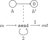
• The constant zero function, $\mathcal {O}: \mathbb {N} \rightarrow \mathbb {N}$, defined by $\mathcal {O} (x) = 0$, for every $x \in \mathbb {N}$, can be computed by the following virus machine $\varPi _{\mathcal {O}}$ with input working in the computing mode:

  • The hosts are $H_{\mathcal {O}} = \{h, h_{\mathrm {zero}}\}$, each of them initially empty.

  • The input host is h and the output host is $h_{\mathrm {zero}}$.

  • The initial and only instruction is halt.

  • Each of the three graphs $D_{H_{\mathcal {O}}}$, $D_{I_{\mathcal {O}}}$ and $G_{C_{\mathcal {O}}}$ determining the functioning of the machine has an empty set of edges.

  This way, for any input the Virus Machine $\varPi _{\mathcal {O}}$ halts in the very first step, and the output host $h_{\mathrm {zero}}$ remains empty. So the output of this machine is always zero.

• The successor function, $\mathcal {S}: \mathbb {N} \rightarrow \mathbb {N}$, defined by $\mathcal {S} (x) = x+1$, for every $x \in \mathbb {N}$, can be computed by the following virus machine $\varPi _{\mathcal {S}}$ with input working in the computing mode:

  • The hosts are $H_{\mathcal {S}} = \{h, h_{\mathrm {one}}\}$, together with the internal hosts of the module ADD(h, $h_{\mathrm {one}}$).

  • The initial contents are zero for the host h and one for the host $h_{\mathrm {one}}$, together with the initial contents of the internal hosts of the module ADD(h, $h_{\mathrm {one}}$).

  • The input host is h and the output host is $h_{\mathrm {one}}$.

  • The instructions are $I_{\mathcal {S}} = \{\mathtt {halt}\}$, together with the instructions of the module ADD(h, $h_{\mathrm {one}}$).

  • The initial instruction is the in instruction of the module ADD(h, $h_{\mathrm {one}}$).

  • The functioning of the Virus Machine is given by the following sequence, which determines the graphs $D_{H_{\mathcal {S}}}$, $D_{I_{\mathcal {S}}}$ and $G_{C_{\mathcal {S}}}$:

    $$\begin{aligned} \mathtt {ADD}(h, h_{\mathrm {one}}) \rightarrow \mathtt {halt} \end{aligned}$$

  This way, for any input the Virus Machine $\varPi _{\mathcal {S}}$ adds it from h to $h_{\mathrm {one}}$ and halts. Since host $h_{\mathrm {one}}$ contained one virus, the output of this machine is equal to the input plus one, as required.

• The projection functions, $\varPi ^{m}_{i} : \mathbb {N}^{m} \rightarrow \mathbb {N}$, with $m \ge 1$ and $1 \le i \le m$, defined by $\varPi ^{m}_{i} (x_{1}, \cdots , x_{m}) = x_{i}$, for every $(x_{1}, \cdots , x_{m}) \in \mathbb {N}^{m}$, can be computed by the following Virus Machine $\varPi _{\varPi ^{m}_{i}}$ with input working in the computing mode:

  • The hosts are $H_{\varPi ^{m}_{i}} = \{h_{1}, \cdots , h_{m}, h_{\mathrm {out}}\}$, together with the internal hosts of the module COPY($h_{i}$, $h_{\mathrm {out}}$).

  • The initial contents are zero for the hosts $h_{1}, \cdots , h_{m}, h_{\mathrm {out}}$, together with the initial contents of the internal hosts of the module COPY($h_{i}$, $h_{\mathrm {out}}$).

  • The input hosts are $h_{1}, \cdots , h_{m}$ and the output host is $h_{\mathrm {out}}$.

  • The instructions are $I_{\varPi ^{m}_{i}} = \{\mathtt {halt}\}$, together with the instructions of the module COPY($h_{i}$, $h_{\mathrm {out}}$).

  • The initial instruction is the in instruction of the module COPY($h_{i}$, $h_{\mathrm {out}}$).

  • The functioning of the Virus Machine is given by the following sequence, which determines the graphs $D_{H_{\varPi ^{m}_{i}}}$, $D_{I_{\varPi ^{m}_{i}}}$ and $G_{C_{\varPi ^{m}_{i}}}$:

    $$\begin{aligned} \mathtt {COPY}(h_{i}, h_{\mathrm {out}}) \rightarrow \mathtt {halt} \end{aligned}$$

  This way, for any input the Virus Machine $\varPi _{\varPi ^{m}_{i}}$ copies the i-th component from $h_{i}$ to $h_{\mathrm {out}}$ and halts, so the output of the machine is that component.

4.4 Composition of Functions

We show now how the composition of functions can be simulated by Virus Machines with input working in the computing mode.

Definition 5

Let and . Then, the composition of f with $g_{1}$ to $g_{m}$, denoted $C(f; g_{1}, \cdots , g_{m})$, is a partial function from $\mathbb {N}^{n}$ to $\mathbb {N}$ defined as follows:

$$\begin{aligned} C(f; g_{1}, \cdots , g_{m}) (x_{1}, \cdots , x_{n}) = f(g_{1}(x_{1}, \cdots , x_{n}), \cdots , g_{m}(x_{1}, \cdots , x_{n})) \end{aligned}$$

for each $(x_{1}, \cdots , x_{n}) \in \mathbb {N}^{n}$.

Let $\varPi _{f}, \varPi _{g_{1}}, \cdots , \varPi _{g_{m}}$ be Virus Machines with input, computing the functions $f, g_{1}, \cdots , g_{m}$, respectively. Let us assume that for each $x \in \{f, g_{1}, \cdots , g_{m}\}$ the elements of the Virus Machine $\varPi _{x}$ are the following:

• The hosts are $H_{x} = \{h_{1}^{x}, \cdots , h_{p_{x}}^{x}\}$.

• The initial contents of the hosts are $n_{1}^{x}, \cdots , n_{p_{x}}^{x}$.

• The input hosts are $h_{1}^{f}, \cdots , h_{m}^{f}$ and $h_{1}^{x}, \cdots , h_{n}^{x}$ for $x \in \{g_{1}, \cdots , g_{m}\}$.

• The output host is $h_{\mathrm {out}}^{x}$.

• The instructions are $I_{x} = \{i_{1}^{x}, \cdots , i_{q_{x}}^{x}\}$.

• The initial instruction is $i_{\mathrm {start}}^{x}$.

• The functioning of the Virus Machine is determined by the directed graphs $D_{H_{x}}$, $D_{I_{x}}$ and the bipartite graph $G_{C_{x}}$.

Then, the composition of f with $g_{1}, \cdots , g_{m}$ can be computed by the following Virus Machine $\varPi _{C(f; g_{1}, \cdots , g_{m})}$ with input:

• The hosts are $H = \{h_{1}, \cdots , h_{n}\} \cup H_{f} \cup H_{g_{1}} \cup \cdots \cup H_{g_{m}}$, together with the internal hosts of the modules.

• The initial contents of the hosts are

  $$\begin{aligned} (0, \cdots , 0, n_{1}^{f}, \cdots , n_{p_{f}}^{f}, n_{1}^{g_{1}}, \cdots , n_{p_{g_{1}}}^{g_{1}}, \cdots , n_{1}^{g_{m}}, \cdots , n_{p_{g_{m}}}^{g_{m}}) \end{aligned}$$

  together with the initial contents of the internal hosts of the modules.

• The input hosts are $\{h_{1}, \cdots , h_{n}\}$.

• The output host is $h_{\mathrm {out}}^{f}$.

• The instructions are $I_{f} \cup I_{g_{1}} \cup \cdots \cup I_{g_{m}} \cup \{\mathtt {halt}\}$, together with the individualized instructions of the modules.

• The initial instruction is the in instruction of the first module.

• The functioning of the Virus Machine is given by the following sequence of concatenated modules, which determines the graphs $D_{H}, D_{I}$ and $G_{C}$:

  • 1. First we simulate the introduction of the input into the input hosts of $\varPi _{g_{1}}$. Recall that the module ADD( $h_{1}$, $h_{2}$ ) does not change the content of host $h_{1}$.

    $$\begin{aligned} \mathtt {ADD}(h_{1}, h_{1}^{g_{1}}) \rightarrow \cdots \rightarrow \mathtt {ADD}(h_{n}, h_{n}^{g_{1}}) \rightarrow \end{aligned}$$

  • 2. We do the same for the machines $\varPi _{g_{2}}, \cdots , \varPi _{g_{m}}$.

    $$\begin{aligned}&\; \rightarrow \mathtt {ADD}(h_{1}, h_{1}^{g_{2}}) \rightarrow \cdots \rightarrow \mathtt {ADD}(h_{n}, h_{n}^{g_{2}}) \rightarrow \\&\qquad \qquad \qquad \qquad \quad \vdots \\&\rightarrow \mathtt {ADD}(h_{1}, h_{1}^{g_{m}}) \rightarrow \cdots \rightarrow \mathtt {ADD}(h_{n}, h_{n}^{g_{m}}) \rightarrow \end{aligned}$$

  • 3. Now we can simulate the functions $g_{1}, \cdots , g_{m}$ over the received input.

    $$\begin{aligned} \rightarrow \varPi _{g_{1}} \rightarrow \cdots \rightarrow \varPi _{g_{m}} \rightarrow \end{aligned}$$

  • 4. Finally, we introduce the outputs of the previous simulations as input for $\varPi _{f}$, simulate f and finish the execution.

    $$\begin{aligned} \rightarrow \mathtt {ADD}(h_{\mathrm {out}}^{g_{1}}, h_{1}^{f}) \rightarrow \cdots \rightarrow \mathtt {ADD}(h_{\mathrm {out}}^{g_{m}}, h_{m}^{f}) \rightarrow \varPi _{f} \rightarrow \mathtt {halt} \end{aligned}$$

4.5 Primitive Recursion of Functions

We show now how the primitive recursion of functions can be simulated by Virus Machines with input working in the computing mode.

Definition 6

Let and . Then, the function obtained by primitive recursion from f and g, denoted Rec(f; g), is a partial function from $\mathbb {N}^{m + 1}$ to $\mathbb {N}$ defined as follows:

$$\begin{aligned} \quad \quad&Rec(f; g) (x_{1}, \cdots , x_{m}, x_{m + 1}) = {\left\{ \begin{array}{ll} f(x_{1}, \cdots , x_{m}), &{} \text {if } x_{m + 1} = 0\\ g(x_{1}, \cdots , x_{m}, x_{m + 1}, y), &{} \text {otherwise} \end{array}\right. }\\&\text {where } y = Rec(f; g) (x_{1}, \cdots , x_{m}, x_{m + 1} - 1) \end{aligned}$$

for each $(x_{1}, \cdots , x_{m}, x_{m + 1}) \in \mathbb {N}^{m + 1}$.

Let $\varPi _{f}$ and $\varPi _{g}$ be Virus Machines with input, computing the functions f and g, respectively. Let us suppose that for each function $x \in \{f, g\}$ the elements of the virus machine $\varPi _{x}$ are the following:

• The hosts are $H_{x} = \{h_{1}^{x}, \cdots , h_{p_{x}}^{x}\}$.

• The initial contents of the hosts are $(n_{1}^{x}, \cdots , n_{p_{x}}^{x})$.

• The input hosts are $h_{1}^{f}, \cdots , h_{m}^{f}$ and $h_{1}^{g}, \cdots , h_{m + 2}^{g}$.

• The output host is $h_{\mathrm {out}}^{x}$.

• The instructions are $I_{x} = \{i_{1}^{x}, \cdots , i_{q_{x}}^{x}\}$.

• The initial instruction is $i_{\mathrm {start}}^{x}$.

• The functioning of the Virus Machine is determined by the directed graphs $D_{H_{x}}$, $D_{I_{x}}$ and the bipartite graph $G_{C_{x}}$.

Then, the function Rec(f; g) can be computed by the following Virus Machine with input $\varPi _{Rec(f; g)}$:

• The hosts are $H = \{h_{1}, \cdots , h_{m + 1}, h', h_{\mathrm {one}}, h_{\mathrm {out}}, h'_{\mathrm {out}}\} \cup H_{f} \cup H_{g}$, together with the internal hosts of the modules.

• The initial contents of the hosts are $0, \cdots , 0, 0, 1, 0, 0, n_{1}^{f}, \cdots , n_{p_{f}}^{f}, n_{1}^{g}, \cdots , n_{p_{g}}^{g}$, together with the initial contents of the internal hosts of the modules.

• The input hosts are $\{h_{1}, \cdots , h_{m + 1}\}$.

• The output host is $h_{\mathrm {out}}$.

• The instructions are $I_{f} \cup I_{g} \cup \{\mathtt {halt}\}$, together with the individualized instructions of the modules.

• The initial instruction is the in instruction of the first module.

• The functioning of the Virus Machine is given by the following sequence of concatenated modules, which determines the graphs $D_{H}, D_{I}$ and $G_{C}$:

  • 1. Observe that to compute the function Rec(f; g) we have to repeatedly compute the function g as many times as indicated by the $(m + 1)$-th argument, except for the first time in which the function f has to be computed instead.

  • 2. First we simulate the introduction of the input for the function f into the input hosts of $\varPi _{f}$.

    $$\begin{aligned} \mathtt {ADD}(h_{1}, h_{1}^{f}) \rightarrow \cdots \rightarrow \mathtt {ADD}(h_{m}, h_{m}^{f}) \rightarrow \end{aligned}$$

  • 3. We now simulate the function f over its input and copy the result to $h_{\mathrm {out}}$ and $h'_{\mathrm {out}}$. This is because if we are done, then the result has to be in $h_{\mathrm {out}}$, but if we are not done, we must pass this result as the last argument to g. However, $h_{\mathrm {out}}$ is required to have out-degree zero, so we take the result from $h'_{\mathrm {out}}$ instead.

    $$\begin{aligned} \rightarrow \varPi _{f} \rightarrow \mathtt {COPY}(h_{\mathrm {out}}^{f}, h_{\mathrm {out}}) \rightarrow \mathtt {COPY}(h_{\mathrm {out}}^{f}, h'_{\mathrm {out}}) \rightarrow \end{aligned}$$

  • 4. We check if we are done, in which case stop the execution.

    $$\begin{aligned} \rightarrow&\mathtt {AREEQUAL?}(h_{m + 1}, h') \mathop {\rightarrow }\limits ^{yes } \mathtt {halt}\\&\downarrow no \end{aligned}$$

  • 5. If we are not done, one computation of g has to be simulated. For that, the $(m + 1)$-th argument of g is updated by adding 1 to it and the appropriate input is introduced into the input hosts of $\varPi _{g}$. The input for the last argument is the result of the previous computation, that we will ensure is always within host $h'_{\mathrm {out}}$.

    $$\begin{aligned}&\mathop {\rightarrow }\limits ^{no } \mathtt {ADD}(h_{\mathrm {one}}, h') \rightarrow \mathtt {ADD}(h_{1}, h_{1}^{g}) \rightarrow \cdots \rightarrow \mathtt {ADD}(h_{m}, h_{m}^{g}) \rightarrow \\&\mathtt {ADD}(h', h_{m + 1}^{g}) \rightarrow \mathtt {ADD}(h'_{\mathrm {out}}, h_{m + 2}^{g}) \rightarrow \end{aligned}$$

  • 6. We simulate the function g and copy the result to both hosts $h_{\mathrm {out}}$ and $h'_{\mathrm {out}}$. Before continuing to step 4, the machine $\varPi _{g}$ has to be restarted to its initial state, so that it can be used to simulate again the function g, if necessary.

    $$\begin{aligned}&\rightarrow \varPi _{g} \rightarrow \mathtt {COPY}(h_{\mathrm {out}}^{g}, h_{\mathrm {out}}) \rightarrow \mathtt {COPY}(h_{\mathrm {out}}^{g}, h'_{\mathrm {out}}) \rightarrow \\&\mathtt {RESTART}(\varPi _{g}) \rightarrow \text {back to step 4} \end{aligned}$$

4.6 Unbounded Minimization of Functions

We show now how the unbounded minimization of functions can be simulated by Virus Machines with input working in the computing mode.

Definition 7

Let . Then, the function obtained by unbounded minimization from f, denoted Min(f), is a partial function from $\mathbb {N}^{m}$ to $\mathbb {N}$ defined as follows:

$$\begin{aligned} Min(f) (x_{1}, \cdots , x_{m}) = {\left\{ \begin{array}{ll} y_{x_{1}, \cdots , x_{m}}, &{} \text {if it exists}\\ \text {undefined}, &{} \text {otherwise} \end{array}\right. } \end{aligned}$$

where

$$\begin{aligned} y_{x_{1}, \cdots , x_{m}} = \min \{y \in \mathbb {N} \, | \,&\forall z < y \, \bigl (f \text { is defined over } (x_{1}, \cdots , x_{m}, z)\bigr ) \, \wedge \\&f(x_{1}, \cdots , x_{m}, y) = 0\} \end{aligned}$$

for each $(x_{1}, \cdots , x_{m}) \in \mathbb {N}^{m}$.

Let $\varPi _{f}$ be a Virus Machine with input, computing the function f. Let us suppose that the elements of the Virus Machine $\varPi _{f}$ are the following:

• The hosts are $H_{f} = \{h_{1}^{f}, \cdots , h_{p_{f}}^{f}\}$.

• The initial contents of the hosts are $n_{1}^{f}, \cdots , n_{p_{f}}^{f}$.

• The input hosts are $h_{1}^{f}, \cdots , h_{m + 1}^{f}$.

• The output host is $h_{\mathrm {out}}^{f}$.

• The instructions are $I_{f} = \{i_{1}^{f}, \cdots , i_{q_{f}}^{f}\}$.

• The initial instruction is $i_{\mathrm {start}}^{f}$.

• The functioning of the Virus Machine is determined by the directed graphs $D_{H_{f}}$, $D_{I_{f}}$ and the bipartite graph $G_{C_{f}}$.

Then, the function Min(f) can be computed by the following Virus Machine with input $\varPi _{Min(f)}$:

• The hosts are $H = \{h_{1}, \cdots , h_{m}, h_{m + 1}, h_{\mathrm {one}}, h_{\mathrm {out}}\} \cup H_{f}$, together with the internal hosts of the modules.

• The initial contents of the hosts are $0, \cdots , 0, 0, 1, 0, n_{1}^{f}, \cdots , n_{p_{f}}^{f}$, together with the initial contents of the internal hosts of the modules.

• The input hosts are $\{h_{1}, \cdots , h_{m}\}$.

• The output host is $h_{\mathrm {out}}$.

• The instructions are $I_{f}\, \cup \{\mathtt {halt}\}$, together with the individualized instructions of the modules.

• The initial instruction is the in instruction of the first module.

• The functioning of the Virus Machine is given by the following sequence of concatenated modules, which determines the graphs $D_{H}, D_{I}$ and $G_{C}$:

  • 1. Observe that to compute the function Min(f) we have to repeatedly compute the function f until we obtain a zero result.

  • 2. First we simulate the introduction of the input for the function f into the input hosts of $\varPi _{f}$.

    $$\begin{aligned} \mathtt {ADD}(h_{1}, h_{1}^{f}) \rightarrow \cdots \rightarrow \mathtt {ADD}(h_{m + 1}, h_{m + 1}^{f}) \rightarrow \end{aligned}$$

  • 3. We now simulate the function f over its input and check if the result is or not zero.

    $$\begin{aligned} \rightarrow \varPi _{f} \rightarrow&\mathtt {ISZERO?}(h_{\mathrm {out}}^{f}) \mathop {\rightarrow }\limits ^{yes }\\&\downarrow no \end{aligned}$$

  • 4. In the case that the result obtained is zero, we copy the last argument to the output host and stop the execution.

    $$\begin{aligned} \mathop {\rightarrow }\limits ^{yes } \mathtt {COPY}(h_{m + 1}, h_{\mathrm {out}}) \rightarrow \mathtt {halt} \end{aligned}$$

  • 5. Otherwise, we add one to the last argument, restart the machine $\varPi _{f}$ so that it can be used again to simulate f, and go back to step 2.

    $$\begin{aligned} \mathop {\rightarrow }\limits ^{no } \mathtt {ADD}(h_{one}, h_{m + 1}) \rightarrow \mathtt {RESTART}(\varPi _{f}) \rightarrow \text {back to step 2} \end{aligned}$$

4.7 Main Result

Taking into account that the class of partial recursive functions coincides with the least class that contains the basic functions and is closed under composition, primitive recursion and unbounded minimization (see [2]), it is guaranteed that it is possible to construct virus machines that compute any partial recursive function. Then, we have the following result.

Theorem 1

The family $NVM(*, *, *)$ equals to the family of all the recursively enumerable sets of natural numbers.

5 Conclusions and Future Work

Virus Machines are a bio-inspired computational paradigm based on the transmissions and replications of viruses [1]. The computational completeness of Virus Machines having no restriction on the number of hosts, the number of instructions and the number of viruses contained in any host along any computation has been established by simulating register machines. However, when an upper bound on the number of viruses present in any host during a computation is set, the computational power of these systems decreases; in fact, a characterization of semi-linear sets of numbers is obtained [1].

The semantics of the model makes it easy to construct specific Virus Machines by assembling small components that carry out a part of the task to be solved. It is then convenient to develop a library of modules solving common problems such as comparisons or arithmetic operations between contents of hosts.

In this paper, Virus Machines able to compute partial functions on natural numbers are introduced. The universality of non-restricted Virus Machines is then proved by showing that they can compute all partial recursive functions.

In [5] Virus Machines working in the generating mode are considered, and it is shown how they can generate any diophantine set, providing, via the MRDP theorem, another proof of the universality of this model of computation. What is interesting is that the structure of the design of these systems has served as inspiration to defined a parallel variant of Virus Machines having several independent instruction transfer networks. It could be interesting to explore other means of introducing parallelism, such as considering more than one type of viruses or allowing more than one virus to be transmitted when a channel is opened.

To study the computational efficiency of this model of computation, for example to analyze if the parallel variants of Virus Machines represent an improvement over the sequential one, a computational complexity theory is required. This way, the resources needed to solve (hard) problems can be rigorously measured.

References

Chen, X., Valencia-Cabrera, L., Pérez-Jiménez, M.J., Wang, B., Zeng, X.: Computing with viruses. Int. J. Bioinspired Comput. (2015, submitted)
Cohen, D.E.: Computability and Logic. Ellis Horwood, Chichester (1987)
Cormen, T.H., Leiserson, C.E., Rivest, R.L.: An Introduction to Algorithms. The MIT Press, Cambridge, Massachussets (1994)
Dimmock, N.J., Easton, A.J., Leppard, K.: Introduction to Modern Virology. Blackwell Publishing, Malden (USA) (2007)
Romero-Jiménez, Á., Valencia-Cabrera, L., Pérez-Jiménez, M.J.: Sequential and parallel generation of diophantine sets by virus machines. J. Comput. Theor. Nanosci. (2015, submitted)
Rozenberg, G., Bäck, T., Kok, J.N.: Handbook of Natural Computing, 1st edn. Springer, Heidelberg (2012)
Acknowledgments
This work was supported by Project TIN2012-37434 of the Ministerio de Economía y Competitividad of Spain, cofinanced by FEDER funds.
Author information
Authors and Affiliations
Corresponding author
Editor information
Editors and Affiliations
Rights and permissions
Copyright information
© 2015 Springer International Publishing Switzerland
About this paper
Cite this paper
Romero-Jiménez, Á., Valencia-Cabrera, L., Riscos-Núñez, A., Pérez-Jiménez, M.J. (2015). Computing Partial Recursive Functions by Virus Machines. In: Rozenberg, G., Salomaa, A., Sempere, J., Zandron, C. (eds) Membrane Computing. CMC 2015. Lecture Notes in Computer Science(), vol 9504. Springer, Cham. https://doi.org/10.1007/978-3-319-28475-0_24
Download citation
DOI: https://doi.org/10.1007/978-3-319-28475-0_24
Published:
Publisher Name: Springer, Cham
Print ISBN: 978-3-319-28474-3
Online ISBN: 978-3-319-28475-0
eBook Packages: Computer ScienceComputer Science (R0)