Extending Naive Bayes Classifier with Hierarchy Feature Level Information for Record Linkage

Abstract

Probabilistic record linkage has been well investigated in recent years. The Fellegi-Sunter probabilistic record linkage and its enhanced version are commonly used methods, which calculate match and non-match weights for each pair of corresponding fields of record-pairs. Bayesian network classifiers – naive Bayes classifier and TAN have also been successfully used here. Very recently, an extended version of TAN (called ETAN) has been developed and proved superior in classification accuracy to conventional TAN. However, no previous work has applied ETAN in record linkage and investigated the benefits of using a naturally existing hierarchy feature level information. In this work, we extend the naive Bayes classifier with such information. Finally we apply all the methods to four datasets and estimate the $F_1$ scores.

Y. Zhou—The authors would like to thank the Tungsten Network for their financial support.

1 Introduction

Record linkage (RL) [1] proposed by Halbert L. Dunn (1946) refers to the task of finding records that refer to the same entity across different data sources. These records contain identifier fields (e.g. name, address, time, postcode etc.). The simplest kind of record linkage, called deterministic or rules-based record linkage, requires all or some identifiers are identical giving a deterministic record linkage procedure. This method works well when there exists a common/key identifier in the dataset. However, in real world applications, deterministic record linkage is problematic because of the incompleteness and privacy protection [2] of the key identifier field.

To mitigate against this problem, probabilistic record linkage (also called fuzzy matching) is developed, which takes a different approach to the record linkage problem by taking into account a wider range of potential identifiers. This method computes weights for each identifier based on its estimated ability to correctly identify a match or a non-match, and uses these weights to calculate a score (usually log-likelihood ratio) that two given records refer to the same entity.

Record-pairs with scores above a certain threshold are considered to be matches, while pairs with scores below another threshold are considered to be non-matches; pairs that fall between these two thresholds are considered to be “possible matches” and can be dealt with accordingly (e.g., human reviewed, linked, or not linked, depending on the requirements). Whereas deterministic record linkage requires a series of potentially complex rules to be programmed ahead of time, probabilistic record linkage methods can be trained to perform well with much less human intervention.

The Fellegi-Sunter probabilistic record linkage (PRL-FS) [3] is one of the most commonly used methods. It assigns the match/non-match weight for each corresponding field of record-pairs based on log-likelihood ratios. For each record-pair, a composite weight is computed by summing each field’s match or non-match weight. When a field agrees (the contents of the field are the same), the field match weight is used for computing the composite weight; otherwise the non-match weight is used. The resulting composite weight is then compared to the aforementioned thresholds to determine whether the record-pair is classified as a match, possible match (hold for clerical review) or non-match. Determining where to set the match/non-match thresholds is a balancing act between obtaining an acceptable sensitivity (or recall, the proportion of truly matching records that are classified match by the algorithm) and positive predictive value (or precision, the proportion of records classified match by the algorithm that truly do match).

In PRL-FS method, a match weight will only be used when two strings exactly agree in the field. However, in many real world problems, even two strings describing the same field may not exactly (character-by-character) agree with each other because of typographical error (mis-spelling). For example, the field (first name) comparisons such as (Andy, Andrew) and (Andy, John) are both treated as non-match in PRL-FS even though the terms Andy and Andrew are more likely to refer to the same person. Moreover, such mis-spellings are not uncommon according to the research results [4] of US Census Bureau, which show that 25 % of first names did not agree character-by-character among medical record-pairs that are from the same person. To obtain a better performance in real world usage, Winkler proposed an enhanced PRL-FS method (PRL-W) [5] that takes into account field similarity (similarity of two strings for a field within a record-pair) in the calculation of field weights, and showed better performance of PRL-W compared to PRL-FS [6].

Probabilistic graphical models for classification such as naive Bayes (NBC) and tree augmented naive Bayes (TAN) are also used for record linkage [7], where the single class variable contains two states: match and non-match. These models can be easily improved with domain knowledge. For example, monotonicity constraints (i.e. a higher field similarity value indicating a higher degree of ‘match’) can be incorporated to help reduce overfitting in classification [8]. Recently, a state-of-the-art Bayesian network classifier called ETAN [9, 10] has been proposed and shown outperform the NBC and TAN in many cases. ETAN relaxes the assumption about independence of features, and does not require features to be connected to the class.

In this paper we will apply ETAN to the probabilistic record linkage problem. Also we will extend the naive Bayes classifier (referred to as HR-NBC) by introducing hierarchy restrictions between features. As discussed in previous work [11, 12], these hierarchy restrictions are very useful to avoid unnecessary computation of field comparison, and to help refine the Bayesian network structure.

In our model, such hierarchy restrictions are mined from the semantic relationships between features, which widely exist in real world record matching problems. An example of this occurs especially in address matching. For example, two restaurants with the same name located in two cities are more likely to be recognized as two different restaurants. Because they might be two different branches in two cities. In this case, the city locations have higher importance than the restaurant names. And we can introduce a connection between these two features.

To deal with mis-spellings in records, we use the Jaro-Winkler similarity function to measure the differences between fields of two records. These field difference values and known record linkage labels are used to train the classifier. Finally, we compare all the methods – PRL-W, TAN, ETAN, NBC and HR-NBC in four datasets. The results show the benefits of using different methods under different settings.

2 Probabilistic Record Linkage

2.1 PRL-FS and PRL-W

Let us assume that there are two datasets A and B of n-tuples of elements from some set F. (In practice F will normally be a set of a strings.) Given an n-tuple a we write $a_i$ for the i-th component (or field) of a.

Matching. If an element of $a \in A$ is the representation of the same object as represented by an element of $b \in B$ we say a matches b and write $a \sim b$. Some elements of A and B match and others do not. If a and b do not match we write $a \not \sim b$. We write $M=\{(a,b) \in A \times B | a \sim b\}$ and $U=\{(a,b) \in A \times B | a \not \sim b\}$. The problem is then, given an element x in $A \times B$ to define an algorithm for deciding whether or not $x \in M$.

Comparison Functions on Fields. We assume the existence of a function:

$$\begin{aligned} cf: F \times F \rightarrow [0,1]. \end{aligned}$$

With the property that $\forall h \in F$, $cf(h,h)=1$. We think of cf as a measure of how similar two elements of F are. Many such functions exist on strings including the normalised Levenshtein distance or Jaro-Winkler. In conventional PRL-FS method, its output is either 0 (non-match) or 1 (match). In PRL-W method, a field similarity score (Jaro-Winkler distance [5, 13]) is calculated, and normalized between from 0 and 1 to show the degree of match.

Discretisation of Comparison Function. Same as previous work [6], rather than concern ourselves with the exact value of $cf(a_i,b_i)$ we consider a set of $I_1, \cdots I_s$ of disjoint ascending intervals exactly covering the closed interval [0, 1]. These intervals are called states. We say $cf(a_i,b_i)$ is in state k to mean $cf(a_i,b_i)\in I_k$.

Given an interval $I_k$ and a record-pair (a, b) we define two values¹:

• $m_{k,i}$ is the probability that $cf(a_i,b_i) \in I_k$ given that $a\sim b$.

• $u_{k,i}$ is the probability that $cf(a_i,b_i) \in I_k$ given that $a\not \sim b$.

Given a pair (a, b), the weight $w_i(a,b)$ of their i-th field is defined as:

where

$$\begin{aligned} w_{k,i}(a,b)= {\left\{ \begin{array}{ll} \ln (\frac{m_{k,i}}{u_{k,i}}) &{}\text { if } cf(a_i,b_i) \in I_k\\ \ln (\frac{1-{m}_{k,i}}{1-{u}_{k,i}})&{} \text { otherwise}. \end{array}\right. } \end{aligned}$$

The composite weight w(a, b) for a given pair (a, b) is then defined as

2.2 The E-M Estimation of Parameters

In practice, the set M, the set of matched pairs, is unknown. Therefore, the values $m_{k,i}$, and $u_{k,i}$, defined above, are also unknown. To accurately estimate these parameters, we applied the expectation maximization (EM) algorithm with randomly sampled initial values for all these parameters.

The Algorithm

• 1. Choose a value for p, the probability that an arbitrary pair in $A \times B$ is a match.

• 2. Choose values for each of the $m_{k,i}$ and $u_{k,i}$, defined above.

• 3. E-step: For each pair (a, b) in $A \times B$ compute

  

  (1)

  where

  $$\begin{aligned} m'_{k,i}(a,b)= {\left\{ \begin{array}{ll} m_{k,i}&{}\text { if } cf(a_i,b_i) \in I_k\\ 1&{} \text { otherwise}. \end{array}\right. } \end{aligned}$$

  and

  $$\begin{aligned} u'_{k,i}(a,b)= {\left\{ \begin{array}{ll} u_{k,i}&{}\text { if } cf(a_i,b_i) \in I_k\\ 1&{} \text { otherwise}. \end{array}\right. } \end{aligned}$$

• 4. M-step: Then recompute $m_{k,i}$, $u_{k,i}$, and p as follows:

  

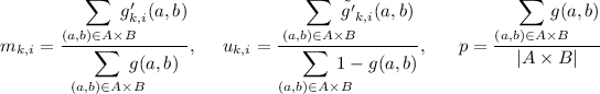  (2)

  where

  $$\begin{aligned} g'_{k,i}(a,b)= {\left\{ \begin{array}{ll} g(a,b)&{}\text { if}\;cf(a_i,b_i) \in I_k\\ 0&{} \text { otherwise}. \end{array}\right. } \end{aligned}$$

  and

  $$\begin{aligned} \tilde{g'}_{k,i}(a,b)= {\left\{ \begin{array}{ll} 1-g(a,b)&{}\text { if}\;cf(a_i,b_i) \in I_k\\ 0&{} \text { otherwise}. \end{array}\right. } \end{aligned}$$

In usage, we iteratively run the E-step and M-step until the convergence criteria are satisfied: $\sum (|\varDelta m_{k,i}|) \le 1\times 10^{-8}$, $\sum (|\varDelta u_{k,i}|) \le 1\times 10^{-8}$, and $|\varDelta p| \le 1\times 10^{-8}$. Having obtained values for $m_{k,i}$ and $u_{k,i}$. We can then compute the composite weight (the natural logarithm of g(a, b)) for each pair defined earlier.

In our implementation, we set the decision threshold as 0.5, and do not consider possible matches. Because using a domain expert to manually examine these possible matches is expensive. Thus, the record-pair (a, b) is recognized as a match if $g(a,b)>0.5$; otherwise it is a non-match.

3 Bayesian Network Classifiers for Record Linkage

In this section we discuss different Bayesian network classifiers (NBC, TAN and ETAN) for record linkage. After that, we discuss the hierarchy structure between features, and the proposed hierarchy-restricted naive Bayes classifier (HR-NBC).

3.1 The Naive Bayes Classifier

Let record-pair feature vector $\overrightarrow{\varvec{f}}$ be an input vector² to the classifier, and $C_{k}$ be a possible class of the binary variable C, where $C_1 = 0$ indicates a non-match and $C_2 = 1$ indicates a match. The model calculates the probability of $C_{k}$ given the feature values (distance for each field-pair). This can be formulated as:

$$\begin{aligned} P(C_k|\overrightarrow{\varvec{f}}) = P(C_k)\times \frac{P(\overrightarrow{\varvec{f}}|C_k)}{P(\overrightarrow{\varvec{f}})} \end{aligned}$$

(3)

Fig. 1.

The graphical representation of NBC, HR-NBC, TAN, ETAN. The blue arrow represents the dependency introduced by hierarchy feature level information.

In the naive Bayes classifier (Fig. 1(a)), we assume the conditional independence of features, $P(\overrightarrow{\varvec{f}}|C_k)$ can be decomposed as . Thus, Eq. (3) becomes:

(4)

With this equation, we can calculate $P(C_k|\overrightarrow{\varvec{f}})$ to classify $\overrightarrow{\varvec{f}}$ into the class (match/non-match) with the highest $P(C_k|\overrightarrow{\varvec{f}})$. This approach is one of the baseline methods we compare our model to.

Like the probabilistic record linkage, one of the often-admitted weaknesses of this approach is that it depends upon the assumption that each of its fields is independent from the others. The tree augmented naive Bayes classier (TAN) and its improved version ETAN relax this assumption by allowing interactions between feature fields.

3.2 The Tree Augmented Naive Bayes Classifier

TAN [14] can be seen as an extension of the naive Bayes classifier by allowing a feature as a parent (Fig. 1(c)). In NBC, the network structure is naive, where each feature has the class as the only parent. In TAN, the dependencies between features are learnt from the data. Given a complete data set $D = \{ D_1, ... , D_L \}$ with L labelled instances, where each instance is an instantiation of all the variables. Conventional score-based algorithms for structure learning make use of certain heuristics to find the optimal DAG that best describes the observed data D over the entire space. We define:

$$\begin{aligned} \hat{G} = \arg \max _{G \in \varOmega } \ell (G,D) \end{aligned}$$

(5)

where $\ell (G,D)$ is the log-likelihood score, which is the logarithm of the likelihood function of the data that measures the fitness of a DAG G to the data D. $\varOmega$ is a set of all DAGs.

Assume that the score (i.e. BDeu score [15]) is decomposable and respects likelihood equivalence, we can devise an efficient structure learning algorithm for TAN. Because every feature $f_i$ has C as a parent, the structure ($f_i$ has $f_j$ and C as parents, $i\ne j$) has the same score with the structure, where $f_j$ has $f_i$ and C as parents:

$$\begin{aligned} \ell (f_i,\{f_j,C\},D) + \ell (f_j,C,D) = \ell (f_j,\{f_i,C\},D) + \ell (f_i,C,D) \end{aligned}$$

(6)

Beside the naive Bayes structure, in the TAN, features are only allowed to have at most one other feature as a parent. Thus, we have a tree structure between the features. Based on the symmetry property (Eq. (6)), we can have an efficient algorithm to find the optimal TAN structure by converting the original problem (Eq. (5)) into a minimum spanning tree construction problem. More details could be found in [9].

3.3 The Extended TAN Classifier

As discussed in the previous section, the TAN encodes a tree structure over all the attributes. And it has been shown to outperform the naive Bayes classifier in a range of experiments [14]. However, when the training data are scarce or a feature and the class are conditionally independent given another feature, we might not get a TAN structure. Therefore, people have proposed the Extended TAN (ETAN) classifier [9, 10] to allow more structure flexibility.

ETAN is a generalization of TAN and NBC. It does not force a tree to cover all the attributes, and a feature to connect with the class. As shown in Fig. 1(d), ETAN could disconnect a feature if such a feature is not important to predict C. Thus, ETAN’s search space of structures includes that of TAN and NBC, and we have:

$$\begin{aligned} \ell (\hat{G}_{ETAN},D) \ge \ell (\hat{G}_{TAN},D) ~~ and ~~ \ell (\hat{G}_{TAN},D) \ge \ell (\hat{G}_{NBC},D) \end{aligned}$$

(7)

which means the score of the optimal ETAN structure is superior or equal to that of the optimal TAN and NBC (Lemma 2 in [9]).

In the ETAN, the symmetry property (Eq. (6)) does not hold, because a feature (e.g. $f_2$ in Fig. 1(d)) is allowed to be disconnected from the class. Thus, the undirected version of minimum spanning tree algorithm cannot be directly applied here. Based on Edmonds’ algorithm for finding minimum spanning trees in directed graphs, people developed the structure learning algorithm of ETAN, whose computational complexity is quadratic in the number of features (as is TAN). For detailed discussions we direct the reader to the papers [9, 10].

3.4 Hierarchy Restrictions Between Features

To utilize the benefits of existing domain knowledge, we extend the NBC method by allowing hierarchy restrictions between features (HR-NBC). These restrictions are modelled as dependencies between features in HR-NBC.

Hierarchy restrictions between features commonly occur in real world problems. For example, Table 1 shows four address records, which refer to two restaurants (there are two duplicates). The correct linkage for these four records is: (1) record 1 and 2 refer to one restaurant in Southwark, and (2) record 3 and 4 refer to another restaurant in Blackheath. As we can see, even record 1 and 3 exactly match with each other in the field of restaurant name, they cannot be linked with each other because they are located in a different borough.

Table 1. Four restaurant records with name, address, borough/town and type information.

Based on the description of the example Table 1, we can see there is a hierarchy restriction between the name and borough fields, where the borough field has higher feature level than name field. Thus, intuitively, it is recommended to compare the borough field first to filter record linkage pairs. To let our classifier capture such hierarchy restriction, we introduce a dependency between these two fields ($f_3 \rightarrow f_1$) to form our HR-NBC model (Fig. 1(b)). Thus, Eq. (4) now becomes:

(8)

Parameter Estimation. Let $\theta$ denote the parameters that need to be learned in the classifier and let r be a set of fully observable record-pairs. The classical maximum likelihood estimation (MLE) finds the set of parameters that maximize the data log-likelihood $\ell (\theta |r)=\log P(r|\theta )$.

However, for several cases in the unified model, a certain parent-child state combination would seldom appear, and the MLE learning fails in this situation. Hence, maximum a posteriori algorithm (MAP) is used to mediate this problem via the Dirichlet prior: $\hat{\theta }=\arg \max _{\theta }\log P(r|\theta )P(\theta )$. Because there is no informative prior, in this work we use the BDeu prior [15] with equivalent sample size (ESS) equal to 1.

4 Experiments

This section compares PRL-W to different Bayesian network classifiers. The goal of the experiments is to do an empirical comparison of the different methods, and show the advantages/disadvantages of using different methods in different settings. Also, it is of interest to investigate how such hierarchy feature level information could improve the classifier’s performance.

4.1 Settings

Our experiments are performed on four different datasets³, two synthetic datasets [12] (Country and Company) with sampled spelling errors and two real datasets (Restaurant and Tungsten). The Country and Company datasets contain 9 and 11 fields/features respectively. All the field similarities are calculated by the Jaro-Winkler similarity function.

Restaurant is a standard dataset for record linkage study [8]. It was created by merging the information of some restaurants from two websites. In this dataset, each record contains 5 fields: name, address, city, phone and restaurant-type⁴.

Tungsten is a commercial dataset from an e-invoicing company named Tungsten Corporation. In this dataset, there are 2744 duplicates introduced by user entry errors. Each record contains 5 fields: company name, country code, address line 1, address line 4 and address line 6.

The experiment platform is based on the Weka system [16]. Since TAN and ETAN can not deal with continuous field similarity values, these values are discretised with the same routine as described in PRL-W. To simulate real world situation, we use an affordable number (10, 50 and 100) of labelled records as our training data. The reason is clear that it would be very expensive to manually label hundreds of records. The experiments are repeated 100 times in each setting, and the results are reported with the mean.

To evaluate the performance of different methods, we compare their ability to reduce the number of false decisions. False decisions include false matches (the record-pair classified as a match for two different records) and false non-matches (the record-pair classified as a non-match for two records that are originally same). Thus these methods are expected to get high precision and recall, where precision is the number of correct matches divided by the number of all classified matches, and recall is the number of correct matches divided by the number of all original matches.

To consider both the precision and recall of the test, in this experiment, we use $F_1$ score as our evaluation criteria. This score reaches its best value at 1 and worst at 0, and is computed as follows:

$$\begin{aligned} F_1 = 2\times \frac{{precision}\times {recall}}{{precision}+{recall}} \end{aligned}$$

(9)

4.2 Results

The $F_1$ score of all five methods in different scenarios are shown in Table 2, where the highest average score in each setting is marked bold. Statistically significant improvements of the best result over competitors are indicated with asterisks * ($p=0.05$).

Table 2. The $F_1$ score of five record linkage methods in different datasets.

As we can see, the PRL-W gets the best result in Company and Restaurant datasets. And its performance does not depends on the number of labelled data. The reason is the record linkage weights were computed with an EM-algorithm as described in Eqs. (1) and (2) over the whole dataset (labelled and unlabelled data). When two classes are easy to distinguish, it is not surprising that the PRL-W could get good performance with limited labelled data.

Because the scarce labelled data and large number of features, TAN and the state-of-the-art ETAN methods have relatively bad performances in Country and Company datasets. Although it is proven that ETAN provides higher fit to the data (Eq. (7)) than TAN, it receives lower classification accuracies in most settings due to overfitting. In the Tungsten dataset, TAN gets the best performance.

According to the results, both NBC and HR-NBC get high $F_1$ scores in all settings. This demonstrates the benefits of using these two methods when the labelled data is scarce. Moreover, the performance of our HR-NBC⁵ is equal or superior to that of NBC in all settings.

5 Conclusions

In this paper, we discussed the hierarchy restrictions between features, and exploited the classification performance of different methods for record linkage on both synthetic and real datasets.

Results demonstrate that, in settings of limited labelled data, PRL-W works well and its performance is independent of the number of labelled data, and show that TAN, NBC and HR-NBC have better performances than ETAN even though the latter method provides theoretically better fit to the data. Compared with NBC, HR-NBC achieves equal or superior performances in all settings, which show the benefits of introducing hierarchy restrictions between features in these datasets.

We note, however, that our method might not be preferable in all cases. For example, in a medical dataset, a patient could move her or his address and have multiple records. In this case, two records with different addresses refer to the same person. Thus, the hierarchy restrictions used in this paper will introduce extra false non-matches.

In future work we will investigate other sources of domain knowledge to enhance the performance of the resultant classifier, such as improving accuracy by using specific parameter constraints [17] elicited from experts.

References

Dunn, H.L.: Record linkage*. Am. J. Public Health Nations Health 36(12), 1412–1416 (1946)
Tromp, M., Ravelli, A.C., Bonsel, G.J., Hasman, A., Reitsma, J.B.: Results from simulated data sets: probabilistic record linkage outperforms deterministic record linkage. J. Clin. Epidemiol. 64(5), 565–572 (2011)
Fellegi, I.P., Sunter, A.B.: A theory for record linkage. J. Am. Stat. Assoc. 64(328), 1183–1210 (1969)
Winkler, W.E.: The state of record linkage and current research problems. In: Statistical Research Division, US Census Bureau, Citeseer (1999)
Winkler, W.E.: String comparator metrics and enhanced decision rules in the Fellegi-Sunter model of record linkage. In: Proceedings of the Section on Survey Research, pp. 354–359 (1990)
Li, X., Guttmann, A., Cipiere, S., Maigne, L., Demongeot, J., Boire, J.Y., Ouchchane, L.: Implementation of an extended Fellegi-Sunter probabilistic record linkage method using the Jaro-Winkler string comparator. In: 2014 IEEE-EMBS International Conference on Biomedical and Health Informatics (BHI), pp. 375–379. IEEE (2014)
Elmagarmid, A.K., Ipeirotis, P.G., Verykios, V.S.: Duplicate record detection: a survey. IEEE Trans. Knowl. Data Eng. 19(1), 1–16 (2007)
Ravikumar, P., Cohen, W.W.: A hierarchical graphical model for record linkage. In: Proceedings of the 20th Conference on Uncertainty in Artificial Intelligence, pp. 454–461. AUAI Press (2004)
de Campos, C.P., Zaffalon, M., Corani, G., Cuccu, M.: Extended tree augmented naive classifier. In: van der Gaag, L.C., Feelders, A.J. (eds.) PGM 2014. LNCS, vol. 8754, pp. 176–189. Springer, Heidelberg (2014)
de Campos, C.P., Corani, G., Scanagatta, M., Cuccu, M., Zaffalon, M.: Learning extended tree augmented naive structures. Int. J. Approximate Reasoning 68, 153–163 (2016)
Ananthakrishna, R., Chaudhuri, S., Ganti, V.: Eliminating fuzzy duplicates in data warehouses. In: Proceedings of the 28th International Conference on Very Large Data Bases, pp. 586–597. VLDB Endowment (2002)
Leitao, L., Calado, P., Herschel, M.: Efficient and effective duplicate detection in hierarchical data. IEEE Trans. Knowl. Data Eng. 25(5), 1028–1041 (2013)
Jaro, M.A.: Advances in record-linkage methodology as applied to matching the 1985 census of Tampa, Florida. J. Am. Stat. Assoc. 84(406), 414–420 (1989)
Friedman, N., Geiger, D., Goldszmidt, M.: Bayesian network classifiers. Mach. Learn. 29(2–3), 131–163 (1997)
Heckerman, D., Geiger, D., Chickering, D.M.: Learning Bayesian networks: the combination of knowledge and statistical data. Mach. Learn. 20(3), 197–243 (1995)
Hall, M., Frank, E., Holmes, G., Pfahringer, B., Reutemann, P., Witten, I.H.: The weka data mining software: an update. ACM SIGKDD Explor. Newslett. 11(1), 10–18 (2009)
Zhou, Y., Fenton, N., Neil, M.: Bayesian network approach to multinomial parameter learning using data and expert judgments. Int. J. Approximate Reasoning 55(5), 1252–1268 (2014)
Author information
Authors and Affiliations
Corresponding author
Editor information
Editors and Affiliations
Rights and permissions
Copyright information
© 2015 Springer International Publishing Switzerland
About this paper
Cite this paper
Zhou, Y., Howroyd, J., Danicic, S., Bishop, J.M. (2015). Extending Naive Bayes Classifier with Hierarchy Feature Level Information for Record Linkage. In: Suzuki, J., Ueno, M. (eds) Advanced Methodologies for Bayesian Networks. AMBN 2015. Lecture Notes in Computer Science(), vol 9505. Springer, Cham. https://doi.org/10.1007/978-3-319-28379-1_7
Download citation
DOI: https://doi.org/10.1007/978-3-319-28379-1_7
Published:
Publisher Name: Springer, Cham
Print ISBN: 978-3-319-28378-4
Online ISBN: 978-3-319-28379-1
eBook Packages: Computer ScienceComputer Science (R0)