Stochastic Games with Signals

Abstract

We survey old and new results concerning stochastic games with signals and finitely many states, actions, and signals. We state Mertens’ conjectures regarding the existence of the asymptotic value and its characterization, and present Ziliotto’s (Ann Probab, 2013, to appear) counter, example for these conjectures.

4.1 Introduction

Stochastic games is a model for dynamic interactions in which the state of nature evolves in a way that depends on the actions of the players. The model was first introduced by Shapley (1953), who proved that two-player zero-sum discounted games have a value and both players have optimal stationary strategies. Bewley and Kohlberg (1976) proved that the limit of the discounted value, as the discount factor goes to 0, exists, and is equal to the limit of the value of the n-stage game, as n goes to infinity. This limit is called the asymptotic value of the game. Mertens and Neyman (1981) further showed that for every ε > 0 Player 1 (resp. Player 2) has a (history dependent) strategy, which guarantees that the payoff in any sufficiently long game, as well as in any discounted game with discount factor sufficiently close to 0, is at least (resp. at most) the asymptotic value minus ε (resp. plus ε). Such a strategy is called uniform ε-optimal.

Mertens et al. (1994) presented a general model of stochastic games with signals, in which the players neither observe the state nor the actions of the other player, but rather observe at every stage a signal that depends on the current state as well as on the pair of actions chosen by the players. Mertens (1986) made the following two conjectures concerning stochastic games with signals and finitely many states, actions, and signals:

• In every stochastic game with signals, the limit of the discounted value, as the discount factor goes to 0, exists, and is equal to the limit of the value of the n-stage game, as n goes to infinity. In other words, the asymptotic value exists.

• If the signal that Player 2 receives is included in the signal that Player 1 receives, then the asymptotic value is equal to the max-min value of the game, which is the maximal quantity that Player 1 can uniformly guarantee in every sufficiently long finite game as well as in every discounted game, provided the discount factor is sufficiently close to 0.

These two conjectures proved to be influential to game theory, and in the attempt to prove them various new tools have been introduced to the field. The conjectures have been shown to hold in quite a few classes of stochastic games with signals (see, e.g., Gensbittel et al. 2014; Neyman 2008; Renault 2006, 2012; Rosenberg 2000; Rosenberg and Vieille 2000; Rosenberg et al. 2002, 2003, 2004; Sorin 1984, 1985; Venel 2014).

Recently Ziliotto (2013) provided an example in which the limit of the discounted value, as the discount factor goes to 0, as well as the limit of the value of the n-stage game, as n goes to infinity, do not exist. In particular, Mertens’ conjectures have been refuted.

In this paper we survey the topic of stochastic games with signals and finitely many states, actions, and signals, with an emphasis on the asymptotic value, and present Ziliotto’s (2013) example.

4.2 Zero-Sum Standard Stochastic Games

4.2.1 The Model

A two-player zero-sum standard stochastic game is described by:

• The set of players I = { 1, 2}.

• A finite state space S.

• For each player i ∈ I and every state s ∈ S, a finite set of actions A ⁱ(s) that are available to player i at state s. The set of action pairs available at state s is A(s): = A ¹(s) × A ²(s), and the set of all pairs (state, action pair) is $\varLambda:=\{ (s,a): a \in A(s)\}$.

• A payoff function $u: \varLambda \rightarrow \mathbb{R}$.

• A transition function $q: \varLambda \rightarrow \varDelta (S)$, where Δ(X) is the set of probability measures over X for every finite set X.

Given an initial state s ₁ ∈ S, the game Γ(s ₁) proceeds as follows. At each stage m ≥ 1, each player chooses an action a _m ⁱ ∈ A ⁱ(s _m ), and a new state s _m+1 is chosen according to the probability measure q(s _m , a _m ), where a _m : = (a _m ¹, a _m ²).

The history up to stage m is the sequence (s ₁, a ₁, s ₂, a ₂, …, s _m ), and the set of all histories of length m is $H_{m}:=\varLambda ^{m-1} \times S$.

In this section we assume perfect monitoring; that is, at the end of each state m the players observe the new state s _m+1 and the pair of actions that were just played a _m . Throughout the paper we assume that players have perfect recall; that is, they do not forget information that they learn along the game. Consequently, a strategy $\sigma ^{i}$ for player i assigns a probability measure over the set of available actions to each finite history. That is, it is a function $\sigma ^{i}: \cup _{m\geq 1}H_{m} \rightarrow \cup _{s\in S}\varDelta (A^{i}(s))$ such that for every $m \in \mathbb{N}$ and every finite history h _m  = (s ₁, a ₁, s ₂, a ₂, …, s _m ) ∈ H _m we have $\sigma ^{i}(h_{m}) \in \varDelta (A^{i}(s_{m}))$. The set of strategies for player i is denoted by $\varSigma ^{i}$ and the set of strategy pairs is $\varSigma:=\varSigma ^{1} \times \varSigma ^{2}$.

An initial state s ₁ ∈ S and a pair of strategies $\sigma \in \varSigma$ induce a probability measure $\mathbb{P}_{s_{1},\sigma }$ over the set of all plays $H_{\infty }:=\varLambda ^{\mathbb{N}}$. The corresponding expectation operator is $\mathbb{E}_{s_{1},\sigma }$. For every discount factor $\lambda \in (0,1]$, the $\lambda$ -discounted payoff under the strategy pair $\sigma$ at the initial state s ₁ is

$$\displaystyle{ \gamma _{\lambda }(s_{1},\sigma ):= \mathbb{E}_{s_{1},\sigma }\left (\sum _{m\geq 1}\lambda (1-\lambda )^{m-1}u(s_{ m},a_{m})\right ). }$$

For every positive integer $n \in \mathbb{N} =\{ 1,2,\ldots \}$, the n-stage payoff under the strategy pair $\sigma$ at the initial state s ₁ is

$$\displaystyle{ \gamma _{n}(s_{1},\sigma ):= \mathbb{E}_{s_{1},\sigma }\left ( \frac{1} {n}\sum _{m=1}^{n}u(s_{ m},a_{m})\right ). }$$

The game $\varGamma _{\lambda }(s_{1})$ is the normal form game $(I,\varSigma ^{1},\varSigma ^{2},\gamma _{\lambda }(s_{1},.))$, and the n-stage game Γ _n (s ₁) is the normal form game $(I,\varSigma ^{1},\varSigma ^{2},\gamma _{n}(s_{1},.))$.

4.2.2 The Value

Definition 1.

Let $\lambda \in (0,1]$ be a discount factor, let $n \in \mathbb{N}$ be a positive integer, and let s ₁ ∈ S be the initial state. The real number $v_{\lambda }(s_{1})$ is the value of the $\lambda$-discounted game $\varGamma _{\lambda }(s_{1})$ if

$$\displaystyle\begin{array}{rcl} v_{\lambda }(s_{1})& =& \max _{\sigma ^{1}\in \varSigma ^{1}}\min _{\sigma ^{2}\in \varSigma ^{2}}\gamma _{\lambda }(s_{1},\sigma ^{1},\sigma ^{2}){}\end{array}$$

(4.1)

$$\displaystyle\begin{array}{rcl} & =& \min _{\sigma ^{2}\in \varSigma ^{2}}\max _{\sigma ^{1}\in \varSigma ^{1}}\gamma _{\lambda }(s_{1},\sigma ^{1},\sigma ^{2}).{}\end{array}$$

(4.2)

The real number v _n (s ₁) is the value of the n-stage game Γ _n (s ₁) if

$$\displaystyle\begin{array}{rcl} v_{n}(s_{1})& =& \max _{\sigma ^{1}\in \varSigma ^{1}}\min _{\sigma ^{2}\in \varSigma ^{2}}\gamma _{n}(s_{1},\sigma ^{1},\sigma ^{2}){}\end{array}$$

(4.3)

$$\displaystyle\begin{array}{rcl} & =& \min _{\sigma ^{2}\in \varSigma ^{2}}\max _{\sigma ^{1}\in \varSigma ^{1}}\gamma _{n}(s_{1},\sigma ^{1},\sigma ^{2}).{}\end{array}$$

(4.4)

When the initial state is chosen according to a probability distribution p ∈ Δ(S), the discounted (resp. n-stage) value is denoted by $v_{\lambda }(p)$ (resp. v _n (p)). In this case, $v_{\lambda }(p) =\sum _{s\in S}p(s)v_{\lambda }(s)$ and $v_{n}(p) =\sum _{s\in S}p(s)v_{n}(s)$, provided the discounted and n-stage values exist for all initial states.

A strategy $\sigma _{{\ast}}^{1} \in \varSigma ^{1}$ (resp. $\sigma _{{\ast}}^{2} \in \varSigma ^{2}$) that attains the maximum (resp. minimum) in Eq. (4.1) [resp. Eq. (4.2)] is called a $\lambda$ -discounted optimal strategy. Similarly, a strategy $\sigma _{{\ast}}^{1} \in \varSigma ^{1}$ (resp. $\sigma _{{\ast}}^{2} \in \varSigma ^{2}$) that attains the maximum (resp. minimum) in Eq. (4.3) [resp. Eq. (4.4)] is called an n-stage optimal strategy.

A strategy is stationary if $\sigma ^{i}(h_{m})$ is a function of s _m , for every $m \in \mathbb{N}$ and every finite history h _m  = (s ₁, a ₁, s ₂, a ₂, …, s _m ) ∈ H _m . A strategy is Markovian if $\sigma ^{i}(h_{m})$ is a function of s _m and m, for every $m \in \mathbb{N}$ and every finite history h _m  = (s ₁, a ₁, s ₂, a ₂, …, s _m ) ∈ H _m . The following two results assert the existence of the value and of stationary (resp. Markovian) optimal strategies in the discounted (resp. n-stage) game.

Theorem 1 (Shapley 1953).

In every standard stochastic game, for every initial state, the $\lambda$ -discounted value exists. Moreover, both players have stationary strategies that are optimal for all initial states.

Theorem 2 (Neumann 1928).

In every standard stochastic game, for every initial state, the n-stage value exists. Moreover, both players have Markovian strategies that are optimal for all initial states.

4.2.3 Zero-Sum Standard Stochastic Games with Long Duration

Considerable effort has been invested on studying properties of stochastic games with long duration, and trying to understand how the value and optimal strategies evolve as the duration goes to infinity. In the discounted game this corresponds to the case where $\lambda$ converges to 0, and in the n-stage game to the case where n goes to infinity.

In other words, we ask whether there is a quantity w that players can guarantee in every discounted game $\varGamma _{\lambda }(s_{1})$, provided $\lambda$ is sufficiently close to 0, and in every n-stage game Γ _n (s ₁), provided n is sufficiently large.

Two approaches can be singled out, the asymptotic approach and the uniform approach. The asymptotic approach assumes that players know the discount factor $\lambda$ (resp. the length of the game n) and that the discount factor is close to 0 (resp. the length is very large). Consequently, this approach is interested in whether the two limits $\lim _{\lambda \rightarrow 0}v_{\lambda }(s_{1})$ and $\lim _{n\rightarrow \infty }v_{n}(s_{1})$ exist and are equal.

The uniform approach assumes that the discount factor is close to 0 (resp. the length of the game is very large), yet it does not assume that players know the discount factor $\lambda$ (resp. the length of the game n). Consequently, this approach is interested in the existence of a strategy that simultaneously guarantees (at least approximately) a payoff greater than $\lim _{\lambda \rightarrow 0}v_{\lambda }(s_{1})$ and $\lim _{n\rightarrow \infty }v_{n}(s_{1})$ in all games $\varGamma _{\lambda }(s_{1})$ and Γ _n (s ₁), provided that $\lambda$ is sufficiently close to 0 and n is sufficiently large.

Definition 2.

A stochastic game Γ has an asymptotic value if (v _n ) and $(v_{\lambda })$ converge (pointwise) to the same limit.

Bewley and Kohlberg (1976) proved that for every initial state s ₁, the function $\lambda \rightarrow v_{\lambda }(s_{1})$ is a semi-algebraic function (thus continuous at 0), and deduced the following theorem.

Theorem 3 (Bewley and Kohlberg 1976).

Any standard stochastic game has an asymptotic value.

Definition 3.

Let s ₁ ∈ S be a state and let $\alpha \in \mathbb{R}$ be a real number. Player 1 (resp. Player 2) can uniformly guarantee α at the initial state s ₁ if for every ε > 0 there exist a strategy $\sigma _{{\ast}}^{1} \in \varSigma ^{1}$ (resp. $\sigma _{{\ast}}^{2} \in \varSigma ^{2}$) and a positive integer $n_{0} \in \mathbb{N}$ such that for every n ≥ n ₀ and every strategy $\sigma ^{2} \in \varSigma ^{2}$ (resp. $\sigma ^{1} \in \varSigma ^{1}$),

$$\displaystyle{ \gamma _{n}(s_{1},\sigma _{{\ast}}^{1},\sigma ^{2}) \geq \alpha -\epsilon \quad (\text{resp.}\quad \gamma _{ n}(s_{1},\sigma ^{1},\sigma _{ {\ast}}^{2}) \leq \alpha +\epsilon ). }$$

(4.5)

The real number α is the uniform value at the initial state s ₁ if both players can uniformly guarantee α at s ₁. A strategy $\sigma _{{\ast}}^{1}$ (resp. $\sigma _{{\ast}}^{2}$) that satisfies (4.5) is called uniform ε-optimal strategy.

The uniform value at the initial state s ₁, when it exists, is denoted by $v_{\infty }(s_{1})$. If a stochastic game has a uniform value at every initial state, then it has an asymptotic value, and both (v _n ) and $(v_{\lambda })$ converge pointwise to $v_{\infty }$ (see Sorin 2002, Chap. 2).

Theorem 4 (Mertens and Neyman 1981).

Any standard stochastic game has a uniform value.

This result extends to a game with random duration, in which the duration is long in expectation and is independent of the play (see Neyman and Sorin 2010).

4.2.4 An Example: The “Big Match”

Consider the following stochastic game, known as the “Big Match”, which was introduced by Gillette (1957). The state space is $S = \left \{\omega,1^{{\ast}},0^{{\ast}}\right \}$, where 1^∗ (resp. 0^∗) is an absorbing state with payoff 1 (resp. 0): in each of these states, each of the players has a single action, say A ¹(1^∗) = { T} and A ²(1^∗) = { L} (resp. A ¹(0^∗) = { T} and A ²(0^∗) = { L}), and once the play moves to state 1^∗ (resp. 0^∗), it remains there: q(1^∗∣1^∗, T, L) = 1 (resp. q(0^∗∣0^∗, T, L) = 1). The action sets for the players in state ω are $A^{1}(\omega ) = \left \{T,B\right \}$ and $A^{2}(\omega ) = \left \{L,R\right \}$. The payoff and transition functions in this state are described in Fig. 4.1.

Fig. 4.1

Transition function (left) and payoff function (right) in state ω

For example, if the action pair (T, L) is played at state ω, then the stage payoff is 1 and the play moves to state 1^∗, where it stays forever. Using Shapley (1953) one can show that $v_{\lambda }(\omega ) = \tfrac{1} {2}$ for every $\lambda \in (0,1]$, and by induction one can show that $v_{n}(\omega ) = \tfrac{1} {2}$ for every $n \in \mathbb{N}$. In particular, the game has an asymptotic value, which is $\tfrac{1} {2}$. The stationary strategy $[\tfrac{1} {2}(L), \tfrac{1} {2}(R)]$ is an optimal strategy for Player 2 in $\varGamma _{\lambda }(\omega )$ and Γ _n (ω), for every $\lambda \in (0,1]$ and every $n \in \mathbb{N}$, and in particular it is a uniform 0-optimal strategy at the initial state ω.

The stationary strategy $[ \tfrac{\lambda }{1+\lambda }(T), \tfrac{1} {1+\lambda }(B)]$ is an optimal strategy for Player 1 in $\varGamma _{\lambda }(\omega )$. The time-dependent strategy that plays at stage t the mixed action $[ \tfrac{1} {n-t+2}(T), \tfrac{n-t+1} {n-t+2}(B)]$ is optimal for Player 2 in Γ _n (ω).

Given ε < 1∕2, constructing a uniform ε-optimal strategy for Player 1 is quite tricky. One can show that Player 1 has no stationary or Markovian strategy that is uniform ε-optimal at the initial state ω, nor does he have a uniform ε-optimal strategy that can be implemented by a finite automaton. It follows from Blackwell and Ferguson (1968) that given a positive integer M, the following history-dependent strategy for Player 1 is uniform $\tfrac{1} {2(2M+1)}$-optimal at ω: at stage m, if the play is at state ω, play T with probability $\tfrac{1} {(M+R_{m}-L_{m})^{2}}$, where R _m (resp. L _m ) is the number of stages up to stage m in which Player 2 played the action R (resp. L). Thus, Player 1 adapts the probability in which he plays T to Player 2’s past behavior: as the difference between the number of times that Player 2 played R and the number of times that he played L increases, Player 1’s total payoff increases as well, and therefore he lowers the probability to play T and end the play at an absorbing state.

4.3 Zero-Sum Stochastic Games with Signals

So far we assumed that players observe both the current state and past choices of the other player. In many situations, this assumption is unrealistic. For instance, if the state represents a resource stock (like the amount of oil in an oil field), the quantity left, which represents the state, can be evaluated, but is not exactly known. Similarly, various decisions of firms that affect the market price are often not observed by other firms. In this section we extend the model of stochastic games with perfect monitoring to the case in which players do not perfectly observe the state or the actions (see Mertens et al. 1994).

4.3.1 The Model

A stochastic game with signals is similar to a standard stochastic game as defined in Sect. 4.2.1 with the following changes:

• There are two finite sets of signals, C for Player 1 and D for Player 2.

• The transition function is a function $q: \varLambda \rightarrow \varDelta (S \times C \times D)$.

At every stage m, each player i chooses an action a _m ⁱ ∈ A ⁱ(s _m ), and a triplet (s _m+1, c _m , d _m ) ∈ S × C × D is drawn according to the probability measure q(s _m , a _m ¹, a _m ²). Player 1 (resp. Player 2) observes the signal c _m (resp. d _m ) and the new state is s _m+1. We emphasize that the only information that Player 1 (resp. Player 2) has at stage m is the initial state

(or the probability distribution according to which the initial state is chosen), the sequence of past actions that he played, and the sequence of past signals that he received.

A history at stage m is a vector (s ₁, a ₁, c ₁, d ₁, s ₂, a ₂, c ₂, d ₂, ⋯ , s _m ) and a play is a vector in $(\varLambda \times C \times D)^{\mathbb{N}}$. Since players have private information, the private history of Player 1 (resp. Player 2) at stage m is $(s_{1},a_{1},c_{1},a_{2},c_{2},\cdots \,,a_{m-1},c_{m-1})$ (resp. $(s_{1},a_{1},d_{1},a_{2},d_{2},\cdots \,,a_{m-1},d_{m-1})$).

Since a player knows the set of actions available for him at every stage of the game, we assume that the private history of a player uniquely identifies his set of actions. For Player 1 this condition translates as follows: for every two histories (s ₁, a ₁, c ₁, d ₁, s ₂, a ₂, c ₂, d ₂, ⋯ , s _m ) and (s′₁, a′₁, c′₁, d′₁, s′₂, a′₂, c′₂, d′₂, ⋯ , s′ _m ), if a _t ¹ = a′ _t ¹ and c _t  = c′ _t for 1 ≤ t < m then A ₁(s _m ) = A ₁(s′ _m ). The condition for Player 2 is analogous.

Many models that have been studied in the literature are special cases of stochastic games with signals. These include:

• 1. Standard stochastic games. These are stochastic games with signals in which the signal contains the new state and the actions that were just played: $C = S \times \left \{\cup _{s\in S}A(s)\right \}$ and $c_{m} = d_{m} = (s_{m+1},a_{m}^{1},a_{m}^{2})$.

• 2. Partially observed Markov decision processes, which are stochastic games with signals that involve only one player: | I | = 1.

• 3. Stochastic games with imperfect monitoring. These are stochastic games with signals in which the signal contains the new state, and possibly additional information: for every s, s′ ∈ S, every a ∈ A(s), every a′ ∈ A(s′), every c ∈ C, and every d ∈ D, if q(c∣s, a) > 0 and q(c∣s′, a′) > 0 then s = s′ (the signal of Player 1 uniquely identifies the state), and if q(d∣s, a) > 0 and q(d∣s′, a′) > 0 then s = s′ (the signal of Player 2 uniquely identifies the state).

• 4. Hidden stochastic games. These are stochastic games with signals in which players receive public signals on the state, and the players observe each other’s action: $C = D = \cup _{s\in S}A(s) \times C'$ and $c_{m} = d_{m} = (a_{m},c'_{m})$.

• 5. Stochastic games played in the dark. These are stochastic games with signals in which the players observe neither the new state nor the action of the opponent: $\vert C\vert = \vert D\vert = 1$.

• 6. Repeated games with incomplete information on both sides. These are stochastic games with signals in which the state does not change along the play and each player receives a private signal about the state at the outset of the game and no further information about the state afterwards.

A strategy for a player is a function that assigns a probability measure over the set of his available actions to every finite private history of the player.

When the game has perfect monitoring, at each stage m the players know the state sm. When the game does not have perfect monitoring, and the signal that a player receives reveals the other player’s action, he can form a belief over the state, which is a probability measure over the set of states S. Consider for example Player 1. At the initial stage his belief over states is the Dirac measure on s ₁. If his belief at stage m is μ _m  ∈ Δ(S), he played the action a _m ¹, Player 2 played the action a _m ² (which he, Player 1, observes), and he observed the signal c _m , then his belief μ _m+1 at the next stage can be calculated by Bayes rule:

$$\displaystyle{\mu _{m+1}(s) = \mathbb{P}(s_{m+1} = s\mid \mu _{m},c_{m},a_{m}^{1},a_{ m}^{2}) = \frac{\sum _{s'\in S}\mu _{m}(s')q(s,c_{m}\mid s',a_{m}^{1},a_{ m}^{2})} {\sum _{s'\in S}q(s,c_{m}\mid s',a_{m}^{1},a_{m}^{2})},}$$

where q(s, c _m ∣s′, a _m ¹, a _m ²) is the marginal probability of (s, c _m ) given (s′, a _m ¹, a _m ²). When the signals of the two players differ, their belief over the state differs as well, and then each player also has a belief over the belief of the other player, each player has a belief over the belief of the other player on his own belief, and so on. This infinite hierarchy of beliefs that arises naturally in stochastic games with signals explains the challenge that their analysis poses. Note that when the signal does not reveal the action of the other player, the player cannot use Bayes rule to calculate his belief, and in fact the player cannot form a belief over the state, unless he knows the strategy used by the other player.

The concepts of asymptotic value, uniform value, and uniform ε-optimal strategies are analogous to the definitions provided above. A natural question is whether stochastic games with signals have an asymptotic value or a uniform value.

By Theorem 1, in the $\lambda$-discounted game each player has a stationary strategy that is optimal for all initial states. Consequently, the $\lambda$-discounted value of a stochastic game with imperfect monitoring is equal to the $\lambda$-discounted value of the same game with perfect monitoring. A similar conclusion holds for the n-stage game, because by Theorem 2, in this game each player has a Markovian strategy that is optimal for all initial states. By Theorem 3 it follows that in stochastic games with imperfect monitoring the asymptotic value exists.

Unfortunately the uniform value may fail to exist in stochastic games with imperfect monitoring. Indeed, consider the “Big Match” and assume that Player 1 observes the state but not the actions of Player 2. Whatever be the signals received by Player 2 about the actions of Player 1, Player 2 can uniformly guarantee $\tfrac{1} {2}$, but he cannot guarantee any quantity lower than $\tfrac{1} {2}$. Player 1, on the other hand, can uniformly guarantee 0 but not any positive quantity.

This leads us to the following definition.

Definition 4.

Let s ₁ ∈ S and let $\alpha \in \mathbb{R}$. Player 2 can uniformly defend α if for every ε > 0 and every strategy $\sigma ^{1} \in \varSigma ^{1}$, there exist a strategy $\sigma _{{\ast}}^{2} \in \varSigma ^{2}$ and a positive integer $n_{0} \in \mathbb{N}$ such that for every n ≥ n ₀,

$$\displaystyle{ \gamma _{n}(s_{1},\sigma ^{1},\sigma _{ {\ast}}^{2}) \leq \alpha +\epsilon. }$$

The real number α is the uniform max-min value at the initial state s ₁ if Player 1 can uniformly guarantee α and Player 2 can uniformly defend α.

The result of Mertens and Neyman (1981) generalizes in the following way (see Rosenberg et al. 2003 or Coulomb 2003):

Theorem 5.

In any stochastic game with imperfect monitoring, the uniform max-min value exists for every initial state. Moreover, the uniform max-min value depends only on the signals that Player 1 gets, that is, on the marginal distribution of q over S × C.

4.3.2 Mertens’ Conjectures

Two natural questions that arise are the following. Does the asymptotic value exist in every stochastic game with signals? If it does, can we characterize it?

Mertens (see Mertens 1986, p. 1572 and Mertens et al. 1994, Chap. VIII, p. 378 and 386) stated two conjectures. The first involves the existence of the asymptotic value in any stochastic game with signals.

Conjecture 1.

Every zero-sum stochastic game with signals has an asymptotic value.

We say that Player 1 is more informed than Player 2 if the signal of Player 1 contains the signal of Player 2. That is, C = D × C′, and c _m  = (d _m , c′ _m ) for every stage m. The second conjecture of Mertens identifies $v_{\infty }$.

Conjecture 2.

In a zero-sum stochastic game with signals where Player 1 is more informed than Player 2, $\lim _{n\rightarrow \infty }v_{n}$ and $\lim _{\lambda \rightarrow 0}v_{\lambda }$ are equal to the max-min value of the game.

The Mertens conjectures have been proven true in numerous special classes of stochastic games with signals, including standard stochastic games (Bewley and Kohlberg 1976; Mertens and Neyman 1981), stochastic games with imperfect monitoring (Rosenberg et al. 2003; Coulomb 2003), repeated games with incomplete information on both sides (Aumann and Maschler 1995; Mertens and Zamir 1971), and partially observed Markov decision processes (Rosenberg et al. 2002). Other classes of stochastic games in which the conjectures have been proven can be found in Gensbittel et al. (2014), Neyman (2008), Renault (2006, 2012), Rosenberg (2000), Rosenberg and Vieille (2000), Rosenberg et al. (2003, 2004), Sorin (1984, 1985), Venel (2014).

Recall that a hidden stochastic game is a stochastic game in which players receive public signals on the state, and the players observe each other’s action. In particular, this is a game in which Player 1 has more information than Player 2. Moreover, in such a game, at every stage both player share the same belief over the state. Ziliotto (2013) provided an example of a hidden stochastic game in which $\lim _{n\rightarrow \infty }v_{n}$ and $\lim _{\lambda \rightarrow 0}v_{\lambda }$ do not exist. This example in particular refutes both of Mertens’ conjectures. We provide this example in the next subsection.

4.3.3 A Counterexample to the Mertens’ Conjectures

Let s ∈ S be a state. We say that Player 1 (resp. Player 2) controls state s if the transition q(s, a ¹, a ²) and the payoff u(s, a ¹, a ²) are independent of a ² for every a ¹ ∈ A ¹(s) (independent of a ¹ for every a ² ∈ A ²(s)).

Consider the following hidden stochastic game Γ, with state space $\left \{1^{{\ast}},1^{++},1^{T},1^{+},0^{{\ast}},0^{++},0^{+}\right \}$, action sets $\left \{C,Q\right \}$ for each player, and signal sets $\left \{D,D'\right \}$ for each player. The payoff function does not depend on the actions, and is equal to 1 in states 1^∗, $1^{++}$, 1^T and 1⁺, and to 0 in states 0^∗, $0^{++}$ and 0⁺. Player 2 controls states $1^{++}$, 1^T and 1⁺. Player 1 controls states $0^{++}$ and 0⁺. States 0^∗ and 1^∗ are absorbing, and the other states are nonabsorbing. Figure 4.2 describes the transition function.

Fig. 4.2

Transitions in the game Γ

In Fig. 4.2 we adopt the following notation: an arrow going from state s to state s′ with the caption $(a,p,c) \in \left \{C,Q\right \} \times [0,1] \times \left \{D,D'\right \}$ indicates that if the player who controls state s plays action a, then with probability p the state moves to state s′ and the signal is c. For example, if the state is $1^{++}$ and Player 2 plays action C, then with probability $\tfrac{1} {2}$ the game moves to state 1^T and the signal is D, and with probability $\tfrac{1} {2}$ the game stays in state $1^{++}$ and the signal is D′.

This game is a hidden stochastic game. As mentioned above, in such a game, at every stage the players share the same belief over the states. In particular, we can consider an equivalent auxiliary stochastic game with perfect monitoring but with countably many states; a state in the auxiliary game corresponds to a belief over states in the original game. Since the number of states, actions, and signals is finite, the number of possible beliefs at each stage is finite, so that in the auxiliary game there are countable many states. By Theorems 1 and 2 (generalized to games with countably many states) in the discounted game the players have optimal stationary strategies and in the n-stage game they have optimal Markovian strategies. Any stationary or Markovian strategy in the auxiliary game has an equivalent strategy in the original game, and vice versa, and therefore the original game and the auxiliary game are equivalent in terms of the discounted value, the n-stage value, and optimal strategies.

Call the states $\left \{1^{{\ast}},1^{++},1^{T},1^{+}\right \}$ 1-states and the states $\left \{0^{{\ast}},0^{++},0^{+}\right \}$ 0-states. In our example, the players know when the play moves from 1-states to 0-states and vice versa. Indeed, the initial state is known, so that the players know whether it is a 1-state or a 0-state. The play moves to a 1-state (resp. 0-state) to a 0-state (resp. 1-state) only when Player 2 (resp. Player 1) plays Q and the signal is D. Consequently the possible beliefs of the players along the play are:

• [1(0^∗)] and [1(1^∗)]: the players know when the play moves to an absorbing state. This is the belief at stage m when the player who controls state s _m−1 played Q and the signal was D′.

• $[2^{-n}(0^{++}),(1 - 2^{-n})(0^{+})]$ for n ≥ 0: players believe that with probability 2⁻ⁿ, the state is $0^{++}$, and with probability $(1 - 2^{-n})$, the state is 0⁺. For n = 0, this is the belief at stage m when (a) the state in stage m − 1 was a 1-state, Player 2 played Q and the signal was D, or (b) the state in stage m − 1 was a 0-state, Player 1 played C and the signal was D′. For n ≥ 1, this is the belief at stage m when the belief at stage m − 1 was $[2^{-(n-1)}(0^{++}),(1 - 2^{-(n-1)})(0^{+})]$, Player 1 played C and the signal was D.

• $[2^{-2n}(1^{++}),(1 - 2^{-2n})(1^{+})]$ for n ≥ 0: players believe that with probability 2⁻²ⁿ, the state is $1^{++}$, and with probability $(1 - 2^{-2n})$, the state is 1⁺. For n = 0, this is the belief at stage m when (a) the state in stage m − 1 was a 0-state, Player 1 played Q and the signal was D, or (b) the state in stage m − 1 was a 1-state, Player 2 played C and the signal was D′. For n ≥ 1, this is the belief at stage m when the belief at stage m − 1 was $[2^{-2n-2}(1^{T}),(1 - 2^{-2n-2})(1^{+})]$, Player 2 played C and the signal was D.

• $[2^{-2n}(1^{T}),(1 - 2^{-2n})(1^{+})]$ for n ≥ 0: players believe that with probability 2⁻²ⁿ, the state is 1^T, and with probability $(1 - 2^{-2n})$, the state is 1⁺. This is the belief at stage m when the belief at stage m − 1 was $[2^{-2n}(1^{++}),(1 - 2^{-2n})(1^{+})]$, Player 2 played C and the signal was D.

To simplify notation, we denote these beliefs as follows:

• 0^∗ is the belief [1(0^∗)]; 1^∗ is the belief [1(1^∗)].

• 0 _n is the belief $[2^{-n}(0^{++}),(1 - 2^{-n})(0^{+})]$.

• 1_2n is the belief $[2^{-2n}(1^{++}),(1 - 2^{-2n})(1^{+})]$.

• 1_2n+1 is the belief $[2^{-2n}(1^{T}),(1 - 2^{-2n})(1^{+})]$.

Thus, the auxiliary game is a stochastic game with perfect information that is given by

• The set of states is {0^∗, 0₀, 0₁, 0₂, 0₃, ⋯ , 1^∗, 1₀, 1₁, 1₂, 1₃, ⋯ }.

• In all states the players have two actions, {C, Q}.

• The payoff in states {0^∗, 0₀, 0₁, 0₂, 0₃, ⋯ } is 0; the payoff in states {1^∗, 1₀, 1₁, 1₂, 1₃, ⋯ } is 1.

• States 0^∗ and 1^∗ are absorbing. The transition function in states {0 _n , n ≥ 0} is described in Fig. 4.3 and the transition function in states {1 _n , n ≥ 0} is described in Fig. 4.4.

  Fig. 4.3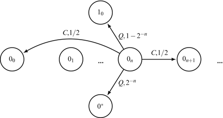

  

  Transitions in the state 0 _n

  Fig. 4.4

  

  Transitions in the states 1_2n and 1_2n+1

We will show below that the limit $\lim _{\lambda \rightarrow 0}v_{\lambda }(s)$ does not exist for every nonabsorbing state of the auxiliary game. We thus consider now the discounted game.

Since the action of Player 2 (resp. Player 1) in states {0₀, 0₁, 0₂, 0₃, ⋯ } (resp. {1₀, 1₁, 1₂, 1₃, ⋯ }) affects neither the payoff nor the transitions, and since the players know the current state of the auxiliary game, for the calculation of the value we can assume that in states {0₀, 0₁, 0₂, 0₃, ⋯ } only Player 1 chooses an action, while in states {1₀, 1₁, 1₂, 1₃, ⋯ } only Player 2 chooses an action. This implies that the decision problems of the two players, namely, the decision problem of Player 1 in states {0₀, 0₁, 0₂, 0₃, ⋯ } and the decision problem of Player 2 in states {1₀, 1₁, 1₂, 1₃, ⋯ }, can be disentangled into two separate Markov decision problems. It follows that in the discounted game each player has an optimal pure stationary strategy. Denote by $\sigma _{n}^{1}$ (resp. $\sigma _{n}^{2}$) the stationary strategy for Player 1 (resp. Player 2) that chooses action C in states {0 _k , k ≠ n} (resp. {1 _k , k ≠ n}) and chooses action Q in state 0 _n (resp. 1 _n ).

Assume that the initial state is p = 0₀. Since the payoff is 1 in states $\{1_{n},\ n \in \mathbb{N}\}$ and 0 in states $\{0_{n},\ n \in \mathbb{N}\}$, and since Player 1 maximizes the payoff, Player 1 wants the play to move to state 1₀. If he plays Q in state 0₀, the game is absorbed in state 0^∗ with probability 1, which is the worst state for him. If he never plays Q, the payoff is 0 forever, which is also an unfavorable outcome for Player 1. If he plays strategy $\sigma _{n}^{1}$, then the play reaches state 0 _n after a random finite number of stages. It is then absorbed in state 0^∗ with probability 2⁻ⁿ (we will call this probability the absorbing risk taken by Player 1), and moves to state 1₀ with probability $(1 - 2^{-n})$.

Inspecting the transition function in Fig. 4.3 reveals that to reach state 0 _n from state 0₀, Player 1 needs on average 2ⁿ stages. Thus, Player 1’s decision of when to play Q is influenced by two contradicting forces: on the one hand he wants to lower the absorbing risk, which means adopting a strategy $\sigma _{n}^{1}$ with high n; on the other hand he wants to minimize the time he spends in states {0₀, 0₁, 0₂, 0₃, ⋯ }, which means he should not choose n too high. Since the game is discounted, the discount factor determines the positive integer n such that $\sigma _{n}^{1}$ is optimal. It turns out that in the $\lambda$-discounted game, the optimal strategies for Player 1 is $\sigma _{n}^{1}$, where 2⁻ⁿ is as close as possible to $\sqrt{2\lambda }$ (the real number $\sqrt{2\lambda }$ corresponds to the optimal absorbing risk if players could choose any absorbing risk in [0, 1], which is not the case).

Player 2 faces the same issue in states {1₀, 1₁, 1₂, 1₃, ⋯ }. However the difference between the transitions in states {1₀, 1₁, 1₂, 1₃, ⋯ } and in states {0₀, 0₁, 0₂, 0₃, ⋯ } leads to a slightly different optimal strategy. We claim that the strategy $\sigma _{2n}^{2}$ is strictly better than the strategy $\sigma _{2n+1}^{2}$. Indeed, both strategies exhibit the same absorbing risk, yet the former requires much fewer stages to move to state 1₀ than the latter. In particular, the optimal strategy of Player 2 is $\sigma _{2n}^{2}$ for some positive integer n. In fact, there exists two mappings $\epsilon _{1},\epsilon _{2}: (0,1] \rightarrow \mathbb{R}$ such that $\lim _{\lambda \rightarrow 0}\epsilon _{1}(\lambda ) =\lim _{\lambda \rightarrow 0}\epsilon _{2}(\lambda ) = 0$, and if $2^{-2n-1+\epsilon _{1}(\lambda )} \leq \sqrt{2\lambda } \leq 2^{-2n+1+\epsilon _{2}(\lambda )}$, then the optimal strategy is $\sigma _{2n}^{2}$.

Set $\lambda _{k}:= 2^{-4k-1}$, so that $\sqrt{ 2\lambda _{k}} = 2^{-2k}$. In the game $\varGamma _{\lambda _{ k}}(1_{0})$ the optimal strategies of the players are $\sigma _{2k}^{1}$ and $\sigma _{2k}^{2}$, and the play is symmetric: the sequence $(v_{\lambda _{k}}(1_{0}))_{k\geq 1}$ converges to $\tfrac{1} {2}$. Set $\mu _{k}:= 2^{-4k-3}$, so that $\sqrt{2\mu _{k}} = 2^{-2k-1}$. In this case, Player 1’s optimal strategy is $\sigma _{2k+1}^{1}$, yet Player 2’s optimal strategy is not $\sigma _{2k+1}^{2}$, because his optimal strategy is taken from the set $\{\sigma _{2n}^{2},n \geq 0\}$. Player 2’s optimal strategy is either $\sigma _{2k}^{2}$ or $\sigma _{2k+2}^{2}$. But choosing $\sigma _{2k}^{2}$ or $\sigma _{2k+2}^{2}$ instead of $\sigma _{2k+1}^{2}$ leads to a different dynamics of the state. For instance, under the strategy $\sigma _{2k+2}^{2}$, starting from state 1₀ Player 2 waits on average 2^2k+2 stages before playing Q, instead of 2^2k+1. Thus, intuitively, Player 1 has an edge over his opponent in the μ _k -discounted game. Standard computations confirm this intuition, and show that $(v_{\mu _{k}}(1_{0}))$ converges to $\tfrac{5} {9}$. In particular, the limit $\lim _{\lambda \rightarrow 0}v_{\lambda }(1_{0})$ does not exist, which implies that the limit $\lim _{\lambda \rightarrow 0}v_{\lambda }(s)$ does not exist for every state in $\{1_{n},n \in \mathbb{N}\}$. Similar arguments show that this limit does not exist for every state in {0 _n , n ≥ 0}.

4.3.4 Link Between the Convergence of (v _n ) and (v _λ )

In the previous example, neither $(v_{\lambda })$ nor (v _n ) converge. There is an example of a hidden stochastic game for which there exists an initial belief p ∈ Δ(S) such that $(v_{\lambda }(p))$ converges but (v _n (p)) does not, and conversely, an example where (v _n (p)) converges and $(v_{\lambda }(p))$ does not converge. Moreover, there are examples in which both $(v_{\lambda }(p))$ and (v _n (p)) converge, but to different limits (Ziliotto 2015). Nonetheless, Ziliotto (2015) proved the following Tauberian theorem, which is a generalization of the one-player case result of Lehrer and Sorin (1992):

Theorem 6.

Consider the auxiliary game of a hidden stochastic game. The following two statements are equivalent:

• 1. For every initial state p ₁ , $\lim _{n\rightarrow \infty }v_{n}(p_{1})$ exists.

• 2. For every initial state p ₁ , $\lim _{\lambda \rightarrow 0}v_{\lambda }(p_{1})$ exists.

Moreover, when these statements hold, we have $\lim _{n\rightarrow \infty }v_{n}(p_{1}) =\lim _{\lambda \rightarrow 0}v_{\lambda }(p_{1})$ for every initial state p ₁ .

This theorem is in fact true in a much wider class of stochastic games with compact state space and actions sets.

4.4 Multiplayer Stochastic Games

A multiplayer stochastic game is similar to a two-player zero-sum stochastic game as defined in Sect. 4.2.1 with the following changes:

• The set of players I is any finite set.

• For every player i ∈ I and each state s, the set A ⁱ(s) is a finite set of actions available to player i at state s. Denote A(s): = × _i ∈ I A ⁱ(s) and $\varLambda:=\{ (s,a): s \in S,a \in A(s)\}$.

• For every player i ∈ I the payoff function is $u^{i}:\varLambda \rightarrow \mathbb{R}$.

In this case we consider the asymptotic behavior of the set $E_{\lambda }(s_{1})$ of all $\lambda$-discounted equilibrium payoffs at the initial state s ₁ and of the set E _n (s ₁) of all n-stage equilibrium payoffs at the initial state s ₁.

4.4.1 Asymptotic Approach

The natural generalization of the result of Bewley and Kohlberg (1976) to the multiplayer case would be the convergence of the set of $\lambda$-discounted Nash equilibrium payoffs $E_{\lambda }$ when $\lambda$ goes to 0 and the convergence of the set of n-stage Nash equilibrium payoffs E _n (w.r.t. the Hausdorff distance).

Note that for a repeated game (that is, a stochastic game with one state) that satisfies certain technical conditions, the Folk theorem answers this question, and gives a characterization of the limit set. A Folk theorem for multiplayer stochastic games has been proven by Dutta (1995), under the strong assumption that the dependence of $E_{\lambda }(s_{1})$ in s ₁ vanishes as $\lambda$ goes to 0 (in particular, this excludes the presence of absorbing states with different payoffs).

In the general case, $E_{\lambda }$ and E _n may fail to converge, even in the two-player case, as proved by Renault and Ziliotto (2014), who prove in addition that the set of discounted (or n-stage) subgame perfect equilibrium payoffs may fail to converge, but the set of discounted stationary Nash equilibrium payoffs converges.

4.4.2 Uniform Approach

The concept of uniform value can be generalized in the following way to the nonzero-sum case.

Definition 5.

A vector $v \in \mathbb{R}^{I}$ is a uniform equilibrium payoff at the initial state s ₁ if for every ε > 0 there exist $\lambda _{0} \in (0,1]$, $n_{0} \in \mathbb{N}$, and a strategy vector $\sigma \in \varSigma$, such that for every player i ∈ I and every strategy $\sigma '^{i} \in \varSigma ^{i}$,

$$\displaystyle{ \gamma _{\lambda }^{i}(s_{ 1},\sigma '^{i},\sigma ^{-i}) - 2\epsilon \leq v^{i}-\epsilon \leq \gamma _{\lambda }^{i}(s_{ 1},\sigma ) \leq v^{i}+\epsilon,\ \ \ \forall \lambda \in (0,\lambda _{ 0}], }$$

and

$$\displaystyle{ \gamma _{n}^{i}(s_{ 1},\sigma '^{i},\sigma ^{-i}) - 2\epsilon \leq v^{i}-\epsilon \leq \gamma _{ n}^{i}(s_{ 1},\sigma ) \leq v^{i}+\epsilon,\ \ \ \forall n \geq n_{ 0}. }$$

Vrieze and Thuijsman (1989) proved the existence of a uniform equilibrium payoff in two-player absorbing games, which are stochastic games with a single nonabsorbing state. Vieille (2000a,b) extended this result to any two-player stochastic game. Flesch et al. (1997) provided an example of a three-player absorbing game in which the uniform equilibrium strategies are periodic. Solan (1999) proved that any three-player absorbing game has a uniform equilibrium in which the players execute a periodic play path, and supplement their play with threats of punishment.

For N ≥ 3, the existence of a uniform equilibrium payoff in multiplayer stochastic games is still open, and is one of the most important and challenging question in mathematical game theory to date. When players are allowed to use a correlation device, this question was solved positively by Solan and Vieille (2002).

4.4.3 Multiplayer Stochastic Games with Imperfect Monitoring

Like in the zero-sum case (see Sect. 4.3), we assume that players do not observe the actions of the other players, but rather receive signals about them. This model is more general than the one of the previous section, thus $(E_{\lambda })$ may not converge (see Renault and Ziliotto 2014). In the literature, Folk theorems for stochastic games with imperfect monitoring are stated under two kinds of assumptions. The first one is an ergodic assumption on the transition function of the game. The second one is either that players do not use their private information [public equilibrium, see Hörner et al. (2011), or public signals, see Fudenberg and Yamamoto (2011)], or an assumption on the signaling function (connectedness, as in Fudenberg and Levine 1991).

4.4.4 Stochastic Games with Signals on the State

When the state is imperfectly observed, it does not seem possible to generalize the result of Bewley and Kohlberg (1976). Indeed, Renault and Ziliotto (2014) provided an example of a two-player hidden stochastic game (public signals on the state and perfect observation of the actions), in which $E_{\lambda }$ has full dimension for all $\lambda \in (0,1]$ (which is a standard assumption in the literature under which Folk theorems are usually stated), but the set of discounted correlated equilibrium payoffs, discounted Nash equilibrium payoffs, discounted sequential equilibrium payoffs, discounted stationary equilibrium payoffs, all fail to converge. Under an ergodic assumption, Yamamoto (2015) recently proved a Folk theorem for multiplayer hidden stochastic games.

References

Aumann RJ, Maschler M (1995) Repeated games with incomplete information. MIT Press, Cambridge
Bewley T, Kohlberg E (1976) The asymptotic theory of stochastic games. Math Oper Res 1(3):197–208
Blackwell D, Ferguson TS (1968) The big match. Ann Math Stat 39(1):159–163
Coulomb J-M (2003) Stochastic games without perfect monitoring. Int J Game Theory 32(1):73–96
Dutta P (1995) A folk theorem for stochastic games. J Econ Theory 66(1):1–32
Flesch J, Thuijsman F, Vrieze K (1997) Cyclic Markov equilibria in stochastic games. Int J Game Theory 26(3):303–314,
Fudenberg D, Levine D (1991) An approximate folk theorem with imperfect private information. J Econ Theory 54(1):26–47
Fudenberg D, Yamamoto Y (2011) The folk theorem for irreducible stochastic games with imperfect public monitoring. J Econ Theory 146(4):1664–1683
Gensbittel F, Oliu-Barton M, Venel X (2014) Existence of the uniform value in repeated games with a more informed controller. J Dyn Games 1:411–445
Gillette D (1957) Stochastic games with zero stop probabilities. Contrib Theory Games 3:179–187
Hörner J, Sugaya T, Takahashi S, Vieille N (2011) Recursive methods in discounted stochastic games: an algorithm for δ → 1 and a folk theorem. Econometrica 79(4):1277–1318
Lehrer E, Sorin S (1992) A uniform Tauberian theorem in dynamic programming. Math Oper Res 17(2):303–307
Mertens JF (1986) Repeated games. In: Proceedings of the international congress of mathematicians, Berkeley, CA, pp 1528–1577
Mertens JF, Neyman A (1981) Stochastic games. Int J Game Theory 10(2):53–66
Mertens JF, Zamir S (1971) The value of two-person zero-sum repeated games with lack of information on both sides. Int J Game Theory 1(1):39–64
Mertens JF, Sorin S, Zamir S (1994) Repeated games. CORE DP 9420–9422
Neyman A (2008) Existence of optimal strategies in markov games with incomplete information. Int J Game Theory 37(4):581–596
Neyman A, Sorin S (2010) Repeated games with public uncertain duration process. Int J Game Theory 39(1):29–52
Renault J (2006) The value of markov chain games with lack of information on one side. Math Oper Res 31(3):490–512
Renault J (2012) The value of repeated games with an informed controller. Math Oper Res 37(1):154–179
Renault J, Ziliotto B (2014) Hidden stochastic games and limit equilibrium payoffs. arXiv preprint arXiv:1407.3028
Rosenberg D (2000) Zero-sum absorbing games with incomplete information on one side: asymptotic analysis. SIAM J Control Optim 39(1):208–225
Rosenberg D, Vieille N (2000) The maxmin of recursive games with incomplete information on one side. Math Oper Res 25(1):23–35
Rosenberg D, Solan E, Vieille N (2002) Blackwell optimality in markov decision processes with partial observation. Ann Stat 30:1178–1193
Rosenberg D, Solan E, Vieille N (2003) The maxmin value of stochastic games with imperfect monitoring. Int J Game Theory 32(1):133–150
Rosenberg D, Solan E, Vieille N (2004) Stochastic games with a single controller and incomplete information. SIAM J Control Optim 43(1):86–110
Shapley LS (1953) Stochastic games. Proc Natl Acad Sci USA 39(10):1095–1100
Solan E (1999) Three-player absorbing games. Math Oper Res 24(3):669–698
Solan E, Vieille N (2002) Correlated equilibrium in stochastic games. Games Econ Behav 38(2):362–399
Sorin S (1984) Big match with lack of information on one side (part i). Int J Game Theory 13(4):201–255
Sorin S (1985) Big match with lack of information on one side (part ii). Int J Game Theory 14(3):173–204
Sorin S (2002) A first course on zero-sum repeated games. In: Mathématiques et applications, vol 37. Springer, Berlin
Venel X (2014) Commutative stochastic games. Math Oper Res 40(2):403–428
Vieille N (2000a) Two-player stochastic games i: a reduction. Isr J Math 119(1):55–91
Vieille N (2000b) Two-player stochastic games ii: the case of recursive games. Isr J Math 119(1):93–126
von Neumann J (1928) Zur theorie der gesellschaftsspiele. Math Ann 100:295–320
Vrieze OJ, Thuijsman F (1989) On equilibria in repeated games with absorbing states. Int J Game Theory 18(3):293–310
Yamamoto Y (2015) Stochastic games with hidden states, preprint, PIER working paper
Ziliotto B (2013) Zero-sum repeated games: counterexamples to the existence of the asymptotic value and the conjecture maxmin= lim v (n). Ann Probab. arXiv preprint arXiv:1305.4778 (to appear)
Ziliotto B (2015) A tauberian theorem for nonexpansive operators and applications to zero-sum stochastic games. arXiv preprint arXiv:1501.06525, Mathematics of Operations Research (to appear)
Acknowledgements
Solan acknowledges the support of grant #323/13 of the Israel Science Foundation. Ziliotto acknowledges the support of the ANR Jeudy (ANR-10-BLAN 0112) and the GDR 2932.
Author information
Authors and Affiliations
Corresponding author
Editor information
Editors and Affiliations
Rights and permissions
Copyright information
© 2016 Springer International Publishing Switzerland
About this chapter
Cite this chapter
Solan, E., Ziliotto, B. (2016). Stochastic Games with Signals. In: Thuijsman, F., Wagener, F. (eds) Advances in Dynamic and Evolutionary Games. Annals of the International Society of Dynamic Games, vol 14. Birkhäuser, Cham. https://doi.org/10.1007/978-3-319-28014-1_4
Download citation
DOI: https://doi.org/10.1007/978-3-319-28014-1_4
Published:
Publisher Name: Birkhäuser, Cham
Print ISBN: 978-3-319-28012-7
Online ISBN: 978-3-319-28014-1
eBook Packages: Mathematics and StatisticsMathematics and Statistics (R0)