
Abstract
Methods to derive an interface concentration profile in a two component system are discussed on the basis of squared gradient theories. Starting point is the description of soft matter systems, where the correlation length of fluctuations becomes the relevant length scale. A phase diagram which contains bulk and interface phase transitions is used as a road map to the involved phenomena. The Landau theory and the Flory-Huggins theory as a typical representative of soft matter mean field theories are outlined as motivations for the squared gradient approach. A brief discussion of bulk properties forms the basis for the discussion of the interface profile of a two component system and the wetting behavior of this system at a substrate.
Access provided by Autonomous University of Puebla. Download chapter PDF
Keywords
These keywords were added by machine and not by the authors. This process is experimental and the keywords may be updated as the learning algorithm improves.
1 Introduction: Soft Matter at Interfaces
This contribution discusses the application of concepts of interface science to a representative soft matter system. While interface science is based on a statistical mechanics language, it usually does not specify a palpable formula for the free energy of a specific system. The concepts thus remain on an abstract and formal level. With an atomistic length scale in mind with detailed and complicated interactions, it might be difficult to write down explicitly a system free energy which is simple enough for further calculations. For soft matter systems, on the other hand, effective statistical mechanical models of suitable simplicity do exist, and thus it is possible to apply the interface formulas. It is not the aim of the soft matter models to describe the atomic length scale, since a description of polymer chains, liquid crystals, or colloids based on first principles would be even more complicated than the description of ensembles based on atoms or low molecular weight molecules. Instead, only the most relevant properties are included in a soft matter model, while other molecular details are summarized as effective parameters. An example are thermotropic nematic liquid crystals, where anisotropic molecules in a liquid state might either self organize with a preferential orientation in a nematic phase, or with random orientation in the isotropic phase. The typical soft matter approach assumes these molecules as rod-like entities with only excluded volume interactions. While such a description simplifies the detailed molecular interactions between the constituent molecules to a maximum extend, it offers a good description of the nematic to isotropic phase transition. The correlation length of fluctuations \(\xi \) becomes the relevant length scale, and a description even of microscopic averages and fluctuations down to this length scale is possible and successful. A second example concerns polymer chains. The most relevant property is here the connectivity of the molecules in a polymer chain, while the molecular interactions are otherwise strongly simplified to excluded volume interactions. The only local parameters of a polymer chain which enter the models are a persistence length \(l_{\mathrm{{ps}}}\) and a molecular friction coefficient. The persistence length of a polymer coil is small for flexible polymer chains, while it is large for stiff polymer chains. The molecular friction coefficient is required to access dynamic phenomena like the relaxation dynamics. On this simplified basis, advanced approaches like the reptation model are able to describe phenomena which are as complicated as the visco-elasticity of polymer melts in rheological experiments.
The application of interface science concepts to soft matter system offers traceable models which describe interfaces on the soft matter length scale \(\xi \). Beside elucidating the interface concepts on specific examples, another important topic of soft matter enters the description of interfaces. For soft matter, suitable degrees of freedom show weak and “soft” restoring forces which are driven by the thermal energy \(k_{\mathrm{{B}}}T\) only. Here, \(k_{\mathrm{{B}}}\) is the Boltzmann constant and T the absolute temperature. An example are again thermotropic liquid crystals. The wide technical use of these systems in liquid crystalline displays relies on the possibility to change the direction of preferred alignment in a nematic phase easily by an electric field of moderate strength. The orientation of this direction which is called liquid crystalline director is a soft degree of freedom.
A simple second example is a rubber band, i.e. a weakly cross-linked polymer melt. A rubber band is easily stretched by moderate mechanical forces. Restoring forces to bring the rubber band back to its original length are caused by entropy elasticity, not by molecular interactions. The stretching of the rubber band is also a soft degree of freedom. It can be stated that the technical important properties of soft matter are mostly due to the soft degrees of freedom in these materials. On this background, a specific question of the SOMATAI initial training network is to identify soft degrees of freedom of these materials at the interface. Those degrees of freedom will react to moderate external forces with a strong response, which might become the starting point of new technological applications.
Which degrees of freedom at interfaces could be soft? So, for which degrees of freedom a deviation from the equilibrium position experiences only weak restoring forces? One can think about a polymer brush, or the two dimensional analog systems of a nematic phase or a polymer melt. And how could we investigate experimentally the softness of these systems? For an answer, we refer to another consequence of softness. Since the restoring forces are weak, the thermal energy \(k_{\mathrm{{B}}}T\) leads to a sizable activation of the soft degrees of freedom. Thus, thermal fluctuations have a significant magnitude in soft matter system. Such fluctuations can be detected by a scattering experiment, in case the fluctuations are connected to the scattering contrast (see Chap. 11 by A. C. Völker et al. and Chap. 12 by J. Daillant). Static scattering experiments yield the root mean squared thermal amplitude of a fluctuation, while dynamic scattering experiments (e.g. dynamic light scattering) provide the relaxation dynamics of a fluctuation, which in many cases is an exponential decay with a relaxation time \(\tau \). The scattering experiment sets up the scattering vector \(\mathbf {q}\), which defines the wave length \(2\pi /|\mathbf {q}|\) and the geometry of the fluctuations. At an interface, it is of importance to distinguish the wavelength \(2\pi /q_{\Vert }\) of a fluctuations within the interface plane, described by the parallel component \(q_{\Vert }\) of \(\mathbf {q}\), and the fluctuation extend perpendicular to the interface. Interface-bound fluctuations which penetrate the bulk only to a limited extend are usually not well characterized by the perpendicular component \(q_{\perp }\) of \(\mathbf {q}\), even if the complex nature of this parameter in interface sensitive scattering experiments is taken into account [1]. Still, \(q_{\perp }\) determines the weighting with which fluctuations with different profiles contribute to a scattering experiment.
Most interfacial degrees of freedom are not soft and are only weakly excited by the thermal energy. An example are capillary waves at a liquid-fluid interface. Since a wave enhances the interface area, capillary waves are suppressed by the interface tension \(\gamma \), especially at short wavelengths (large \(q_{\Vert }\)). For large wavelengths, it is the density difference between the two phases which suppresses capillary waves and yields a flat, horizontally oriented interface. For extremely low interface tension, also capillary waves become soft and reach a sizable thermal amplitude [2]. In liquid crystalline displays, it is the non-soft interface anchoring of the preferred nematic orientation at the interfaces of a display device which provides the restoring force for the bulk orientation.
A suitable soft matter system to elucidate and study concepts of interfacial science and interfacial fluctuations are mixtures of polymers A and B, described by the Flory-Huggins theory. Depending on the interaction strength between the two polymers which form the mixture, there is either a one-phase, mixed system, or a phase separation into two phases. The theory is usually applied for the description of bulk phases, or phase de-mixing kinetics in the bulk. Here, we study interface effects of the theory. The mixture is brought in contact with an interface of a third material, and the wetting transitions between partial and complete wetting will be investigated. For partial wetting, a non-zero contact angle is formed, while complete wetting is characterized by contact angle zero. Furthermore, there are internal interfaces between the two phases. Depending on the width of the interface region, one distinguishes a weak segregation limit (WSL) with a smooth transition, a strong segregation limit (SSL) with a more sharp transition and even a super strong segregation limit (SSSL) with a step-like concentration change. These cases are also important in the description of block-copolymer systems, where A and B are not separate polymer coils, but linked blocks of a common polymer coil.
For a theoretical description of soft matter systems, the application of mean-field theories offers a first approach. These theories are often based on intuitive arguments. The implemented physical mechanisms which determine the behavior of a theory can thus be followed directly. The essential simplification in a mean field theory is the introduction of the mean field, which covers the multi-particle interactions of the constituents on a simplified basis. These interactions are pre-averaged, and form the mean field. The theoretical description of a complicated many particle system is reduced in this way to the description of the single particle behavior in the presence of the mean field. The single particle behavior is dependent on the strength of the mean field. On the other hand, the strength of the mean field is a suitable average over the single particle behavior. The combination of these two dependencies leads to an equation, where the mean field is calculated as an average which depends on the mean field. This closure of the mean field theory is the essential step, and its solution is called a self-consistent solution. We can take advantage of the common background of mean field theories for different soft matter classes and will apply concepts which were developed for liquid crystals to polymer mixtures described by the Flory-Huggins theory.
The mean field concept fails when the description by averaged interactions is not appropriate. This situation happens when there are large fluctuations within a system, especially very close to a second order phase transition, which is also called a critical point. Another system known to have large fluctuations is a semi-dilute polymer solution. Due to the large fluctuations, the concept of an averaged local mean field is no longer appropriate and no longer successful. Very close to a critical point, there is interesting physics which can be described by different theoretical concepts, e.g. scaling arguments. By inverting the failure argument of mean field theories into a positive criterion it can be stated, that apart from conditions very close to critical points and other possible situations with strong fluctuations, mean field theories describe a soft matter system usually rather well. This finding might be traced back to a coincidence: for technical applications, we are mainly interested in systems with soft matter properties around room temperature. The temperature of the critical point \(T_{\mathrm{{cp}}}\) is usually also in this range, let’s say around \(T_{\mathrm{{cp}}}\sim \text {300 K}\). When we perform measurements with a temperature deviation \(\varDelta T\) from the critical point, the relative deviation \(\varDelta T/T_{\mathrm{{cp}}}\) typically remains small. A deviation of \(\varDelta T\sim 60\,\mathrm {K}\) which would be an impressing range for a nematic phase might appear large at first sight, however, the correlation length of fluctuations is still enhanced compared to the molecular length scale by the proximity of the critical point \(\varDelta T/T_{\text{ cp }}\sim 0.2\). Thus, a theoretical description on the length scale \(\xi \) based on suitable averages of molecular interactions is sufficient and successful. On this basis, it is expected that soft matter interfaces can also be described successfully down to a length scale \(\xi \) by mean field theories, as long as one does not approach the critical point too closely. Equivalent to mean field theories is the Landau theory, or the squared gradient theory introduced by van der Waals.
The outline of this contribution is as follows: as a start, Sect. 8.2 provides an introduction to wetting transitions, with a general phase diagram of bulk and interface phase transitions. As a second step, the Landau theory and the Flory-Huggins theory are briefly introduced in Sect. 8.3, as examples of squared gradient theories. The Flory-Huggins theory describes a similar phase diagram, where, however, the temperature is replaced by the interaction parameter \(\chi \). For the equivalent Cahn Hilliard theory, only few literature hints will be provided. Since interfaces are boundaries of a bulk phase, a brief outline of bulk properties in Sect. 8.4 forms the basis of a discussion of interfaces, which will be treated in Sect. 8.5. A general approach for the calculation of interface properties within the squared gradient theories is illustrated for the Landau theory.
2 Wetting Transitions
The phase diagram of a binary mixture might serve as a roadmap to interfacial phenomena. Such a mixture is composed of two constituents A and B. Volume additivity is assumed and the volume V contains the volume fraction \(\phi \) of B and \(1-\phi \) of A. Attractive interactions are usually stronger between molecules of the same kind [3], and thus the internal energy contribution U to the free energy \(F=U-TS\) favors a de-mixing of the mixture. The entropic contribution S, on the other hand, is higher in a mixed state. Since the entropy is weighted with the temperature T, it wins at high T and there is generally a mixed state at high T. At low T, interactions might lead to a de-mixing. We follow the discussion of Bonn and Ross for the description of wetting phenomena [4], and combine it with physical arguments provided by Strobl [5]. The shape of the phase diagram is depicted in Fig. 8.1.

Phase diagram of a binary mixture. The bulk behavior is illustrated by black lines, while the interface behavior is drawn in grey. The left two insets illustrate the cases of complete wetting for a temperature above the wetting temperature \(T_{\mathrm{{w}}}\) and partial wetting for \(T<T_{\mathrm{{w}}}\). The right inset displays the difference between a thick and a thin interface layer, which occur at the left and the right side of the pre-wetting line, respectively
2.1 Bulk Behavior of the Mixture
We first focus on the black lines and labels in Fig. 8.1 which indicate the bulk behavior of the mixture. In the shaded one phase region, the A-B blend is in the mixed state. The border to the de-mixed state is indicated by a line which is called binodal \(T_{\mathrm{{bin}}}(\phi )\). A system prepared at a point \((\phi ,T)\) which falls into the two phase region is not thermodynamically stable. Phase separation sets in and two phases are created. One phase is rich in A and the other rich in B. Entropy effects are still present and no pure phases are created in general. The resulting compositions of the two phases are found on the two points of the binodal curve which are at the temperature set by the experiment. So, for a system prepared at point \((\phi ,T)\) in the two phase region, one finds the compositions of the two resulting phases by moving at the same T to the left and to the right until the binodal is hit. In order to find the volumes occupied by the A-rich phase and the B-rich phase, one can use the known compositions of the de-mixed phases and determine the volumes of the A-rich phase and the B-rich phase in a way so the total content of A and B match the original preparation conditions \((\phi ,T)\).
The spinodal line \(T_{\mathrm{{spin}}}(\phi )\) in the two phase range separates two regions with different mechanisms of phase separation. In the region between the binodal and the spinodal, the mixture is meta-stable. It might remain mixed for a while, although the mixed state is not the thermodynamic equilibrium. Phase separation occurs here via nucleation and growth. A thermal fluctuation might lead to a large enough volume element with surplus of one component, let’s say A. This fluctuation acts as a nucleation point which can initiate a phase separation of the whole system. The formation of such a nucleus involves the creation of an interface between the A-rich fluctuation and the remaining system. A small nucleus has an unfavorable interface to volume ratio and so the fluctuation rather decays than initiates the phase separation. Only if the fluctuations produce a large enough nucleus it survives and initiates macroscopic phase separation. Note, that this mechanism of meta-stability involves interface effects between the nucleus and the surrounding. The meta-stability indicates, that the de-mixing is a first order phase transition.
In the region below the spinodal, a mixture is unstable and decays immediately. Concentration fluctuations of all wavelengths no longer have restoring forces, but are even enhanced by thermodynamics which favors de-mixing for these unstable situations. The interplay of diffusion which requires more time to set up a concentration fluctuation of large wavelength and thermodynamic driving force which increases with the wavelength of a fluctuation results in a de-mixing, where the wavelength of the fastest growing concentration fluctuation sets the length scale where de-mixing starts. In later stages of de-mixing, there is a coarse graining and building up of better defined interfaces between A-rich and B-rich regions.
The binodal and the spinodal meet in the phase diagram in the bulk critical point. In this point, the de-mixing becomes a second order phase transition. It is here that strong concentration fluctuations occur, since restoring forces are weak. In the region very close to the critical point, mean-field theories are no longer suitable and scaling arguments can predict the right behavior. When approaching the critical point, the difference in the A-rich phase and the B-rich phase gets smaller and finally vanish (recall that the de-mixing process leads to an A-rich phase and a B-rich phase which are the two points of the binodal at the same temperature as the original instable mixed state; at the critical point, the compositions of these phases become identical). For a temperature above the critical phase transition temperature, a distinction between the two phases is no longer possible. The situation is in analogy to the critical point of a single phase system. When the pressure is varied, the first order boiling transition becomes second order at the critical pressure, and for higher pressure it is no longer possible to distinguish liquid and vapor. The bulk critical point is of special interest for experimentalists. At this value of \(\phi \), a T jump starting from the one phase region to the two phase region directly reaches a composition where spinodal de-mixing can be observed, without the necessity to cross a region of nucleation and growth in the T-jump.
2.2 Interface Behavior of the Mixture
When the binary mixture gets into contact with a substrate—either the container, a test sample, a colloidal particle, or a gas phase—either A or B molecules are preferentially absorbed at the interface. The interface behavior of the mixture is included to Fig. 8.1 in grey color [6], where we assume that the interactions result in a preferable adsorption of A to the interface. The two phase region is split by the horizontal wetting line, which separates regions of partial and complete wetting. For complete wetting, a film of macroscopic thickness of one phase covers the interface—for our assumption of preferential adsorption of A molecules it is the A-rich phase. For partial wetting, the interface might be covered by a microscopic thin film of the component with preferential adsorption, however, no homogeneous film of macroscopic thickness evolves. Instead, drops of the preferentially adsorbed phase are observed at the interface. The ‘Cahn argument’ established by Cahn in 1977 indicates, that close to the bulk critical point there is always complete wetting [6]. The transition of partial to complete wetting is an interface phase transition. Usually, it is of first order, which implies a sudden, non-steady change in the thickness of the absorbed layer from microscopic to macroscopic thickness. A further consequence of the first order nature of this interface phase transition is the existence of meta-stable states, so a meta-stable microscopic thin film and partially wetted interface for \(T>T_{\mathrm{{w}}}\) or a meta-stable macroscopically thick film for \(T<T_{\mathrm{{w}}}\) (as a bulk analogy consider the first order boiling transition of water, where superheating of water and supercooling of vapor in the absence of nucleation sites are possible meta-stable states). Also a thermodynamic contribution (beside pinning) for the difference in advancing and receding contact angles of a liquid drop on a solid substrate can be discussed on the basis of meta-stability. The Cahn argument was discussed by Bonn and Ross, who also reviewed scientific papers describing a continuous wetting transition which can be achieved under certain, suitable conditions.
The preferential adsorption of one component to the substrate persists into the one phase region. The typical size of thermal fluctuations of the local composition defines the correlation length \(\xi \). This length is small and compares to molecular dimensions for a location \((\phi ,T)\) far away from the bulk critical point, however, it increases and diverges when approaching the bulk critical point. The preferential adsorption of one component at a substrate can be compared to a bulk fluctuation, and so the thickness of a resulting interface layer is equal to \(\xi \). More exactly, an exponential concentration profile is found at the interface with a decay length equal to \(\xi \). Close to the bulk critical point where fluctuations become enhanced, the preferential interface adsorption of one component can thermodynamically stabilize a fluctuation, and an interface layer with thickness larger than \(\xi \) evolves. For our assumption of preferential A adsorption to the substrate, such thick layers are found on the B-rich side of the phase diagram in Fig. 8.1 in case the temperature is larger than the pre-wetting temperature \(T_{\mathrm{{pw}}}\) and only slightly above \(T_{\mathrm{{bin}}}(\phi )\). The interface phase transition within the bulk one-phase region between a thin film with thickness \(\xi \) and a thick film is called pre-wetting transition. It can be either a first or second order transition, or a supercritical change. When changing \(\phi \), the first order pre-wetting transition occurs for different temperatures. The trace of these temperatures of first order pre-wetting transitions is captured by the pre-wetting line. The pre-wetting line ends at the critical pre-wetting point, where the pre-wetting transition becomes a second order phase transition. For compositions \(\phi \) closer to the bulk critical point and higher temperatures, there is a super-critical continuous change from a thin to a thick layer. In Fig. 8.1, the starting temperature \(T_{\mathrm{{pw}}}\) of the pre-wetting line is distinguished from \(T_{\mathrm{{w}}}\). Usually, these two temperatures coincide, and in this case the wetting transition is of first order. It turns out, however, that for the Landau theory which is discussed as main example in Sect. 8.5.2 a different behavior with \(T_{\mathrm{{w}}}<T_{\mathrm{{pw}}}\) is encountered. For this case, there is no jump in the contact angle like in a first order wetting transition, but a continuous change from zero to finite values.
A broad overview over the interface behavior of polymers also from the experimental side is provided by the book of Jones and Richards [7]. Examples of experimental and theoretical results of wetting on colloidal particles are found in references [8, 9].
2.3 The Contact Angle
For completeness, the connection between contact angle and interface tension is briefly repeated. The interface tension \(\gamma \) between two phases can be expressed either as specific interface energy with the dimension energy per interface area, or as force per width. The second option, which indicates the required force to increase the size of an interface of fixed width is used to motivate the Young Dupre equation
Here, \(\gamma _{\mathrm{{ab}}}\), \(\gamma _{\mathrm{{aS}}}\), and \(\gamma _{\mathrm{{bS}}}\) are the interface tensions between the A-rich phase and the B-rich phase, the A-rich phase and the substrate, and the B-rich phase and the substrate, respectively. For the usage of indices, we generally use capital letters A and B for the pure A and B phase only, while the A-rich and the B-rich phases are indicated by the lower case letters a and b. The contact angle inside the A-rich droplet is denoted as \(\varTheta _{\mathrm{{a}}}\). Figure 8.2 illustrates the acting forces: the force per width to the left composed of \(\gamma _{\mathrm{{aS}}}\) and the component parallel to the interface \(\gamma _{\mathrm{{ab}}}\cos (\varTheta )\) is counter balanced by the force per area \(\gamma _{\mathrm{{bS}}}\) to the right. Only for \(\gamma _{\mathrm{{bS}}}<\gamma _{\mathrm{{aS}}}+\gamma _{\mathrm{{ab}}}\), (8.1) can be used for the calculation of the contact angle, while for \(\gamma _{\mathrm{{bS}}}>\gamma _{\mathrm{{aS}}}+\gamma _{\mathrm{{ab}}}\) complete wetting of the A-rich phase occurs. This relation is the basis for the spreading coefficient of the A-rich phase
For a positive value of \(S_{\mathrm{{a}}}\), a drop of A-rich phase will tend to cover the interface to the substrate. For any contact of the B-rich phase with the substrate, the interface energy can be reduced by replacing the interface of the substrate to B-rich phase by two interfaces, one of them substrate to A-rich phase and the other one A-rich phase to B-rich phase. In analogy to (8.2), a spreading coefficient \(S_{\mathrm{{b}}}\) for the B-rich phase can be defined in order to decide, if there is complete or partial wetting of the substrate by the B-rich phase. Here, we always assume that the A-rich phase preferentially adsorbs to the substrate. Bonn and Ross argue that the spreading coefficient in equilibrium cannot attain positive values, since any contact of the B-rich phase will have been eliminated after complete wetting [4]. Such a concept does not fit to the definition (8.2), but rather an alternate quantity defined as \(S_{\mathrm{{a}}}^{\prime }=\text {min}\left( S_{\mathrm{{a}}},0\right) \). We stick to (8.2) as definition, interpret the spreading coefficient as thermodynamic tendency to wet an interface, and tolerate positive values of \(S_{\mathrm{{a}}}\). Meta-stable partial wetting states and pinning can lead to situations with positive \(S_{\mathrm{{a}}}\) without complete wetting.

Balance of the force per length of an A-rich phase and a B-rich phase at a solid substrate S
3 Squared Gradient Theories
There are several approaches to justify the phenomenological description of Sect. 8.2 and the roadmap of Fig. 8.1. On a mean-field level and for short ranged interactions, they typically lead to an increment of a thermodynamic potential of the form:
Here, \(\varDelta \varOmega \) is an increment of the grand canonical potential and \(\varDelta \omega \) is its density, so the grand canonical potential increment of a volume element divided by the size of this element. The free energy increment \(\varDelta F\) can be expressed by the free energy density \(\varDelta f\) and the squared gradient of \(\phi \) similar to (8.3). In the description based on increments \(\varDelta \varOmega \) or \(\varDelta F\) it is not required, to consider other contributions which are independent of \(\phi \). Any constant background terms in addition to these increments do not affect the subsequent calculations which are based on derivatives of \(\varDelta \varOmega \) or \(\varDelta F\). The result of (8.3) depends on the composition profile \(\phi (\mathbf {r})\), as indicated by the squared brackets on the left side. A system optimizes \(\phi (\mathbf {r})\) for a minimal value of \(\varDelta \varOmega \) or \(\varDelta F\). A brief introduction to the mathematical tools to perform this optimization is provided in the appendix, Sect. 8.8.
Interactions between neighboring volume elements are considered by the second term in the integral (8.3), which involves a phenomenological elastic constant \(\kappa \). In bulk, a system in thermodynamic equilibrium is in a homogeneous state, i.e. a state with a constant value of \(\phi \) for all locations \(\mathbf {r}\) and thus vanishing gradient \(\nabla \phi \) everywhere. Deviations from a homogeneous \(\phi \) result in a higher value of \(\varDelta \varOmega \). The increase in \(\varDelta \varOmega \) for inhomogeneous states is described by the square of \(\nabla \phi \) in (8.3). The square can be considered as the second term in a Taylor expansion, where the zero and first order terms vanish in order to match the condition of minimum bulk value of \(\varDelta \varOmega \) for a homogeneous state. Since only short range interactions are assumed in the theory, higher terms in the Taylor series can be neglected. In different fields, (8.3) is addressed either as Landau-Ginzburg functional [5], or squared gradient theory [4], which is traced back to van der Waals. This section provides an overview over two famous approaches which lead to (8.3). A third approach with very similar arguments is the Cahn Hilliard theory [10–12]. A historical overview and an application to simulations is described by Lamorgese et al. [13].
3.1 Landau Theory
Landau Free Energy Density The canonical approach to statistical mechanics (see also Chap. 7 by W.J. Briels and J.K.G. Dhont) starts with the calculation of the partition function Z, and the free energy F results as
Here, \(k_{\mathrm{{B}}}\) is the Boltzmann constant. When the system is divided to cells, and \(E_i\) denotes the energy contained in cell i, Z reads [14]
Instead of the sum over the cells, one can integrate over the distribution \(\rho \) of \(\phi \) values in the system
An improvement of (8.6) takes interactions between the cells into account. Due to the assumed short range nature of the interactions, it is sufficient to consider interactions between neighbouring cells. The interaction between two neighboring cells scales with the difference of their \(\phi \) values divided by the cell size. For neighboring cells with identical \(\phi \), the interaction is zero, while a deviation in \(\phi \) leads to a positive contribution. In the limit of infinitesimal small cell size, this parameter reduces to the derivative \(\nabla \phi \) of \(\phi (\mathbf {r})\). The weighted sum over different profiles \(\phi (\mathbf {r})\) is achieved by a functional integration \(\mathbf{D}\phi (\mathbf {r})\) over different profiles \(\phi (\mathbf {r})\), which leads to
The function
which is called Landau free energy density, takes energetic contributions \(E(\phi )\) and entropic contributions \(k_{\mathrm{{B}}}T\ln (\rho (\phi ))\) into account. Inhomogeneities are considered in (8.7) by the gradient term \(E'(\phi ,\nabla \phi ,\,T)\). The latter can be expressed as a Taylor series in \(\nabla \phi \). The zero order term of this series vanishes, as the interaction between neighboring cells with the same \(\phi \) is zero. The first order term as well as higher odd order terms can be excluded by a symmetry argument. If they would have a non-zero value, it could be reverted by mirroring the coordinates. Since the thermodynamic properties do not depend on the choice of the coordinates, such contributions can be excluded. For weak gradients, \(E'(\phi ,\nabla \phi ,\,T)\) is usually reduced to the second order term \(\frac{1}{2}\kappa (\nabla \phi )^2\), which leads to the squared gradient term in (8.3). The elastic constant \(\kappa \) might depend on \(\phi \) and T.
It is now required to show that F in the conventional equation (8.4) and the integration over f have the same information content. With this equivalence, it is possible to consider f as a free energy density and to discuss a system based on f instead of F. The exponential function in (8.7) is at maximum for the value of \(\phi \) which yields the minimum value of f. The maximum is very sharp, since the integration in the exponential function is over V, which can be made very large in the thermodynamic limit. Any deviation from the minimum of f is multiplied by a large volume factor and weighted exponentially. For this reason, the sharp maximum of the exponential function and thus the minimum of f dominate the integration in (8.7) and thus determine the thermodynamic behavior of the system.
As a quantitative example, we consider the homogeneous mixed bulk state described by the equilibrium value \(\phi _{\mathrm{{eq}}}\). It is not required to consider the squared gradient term in the discussion of the bulk equilibrium, since this term increases f for inhomogeneous states, which are thus away from the minimum of f. Due to this simplification, the functional integration in (8.7) is only over constant paths and thus reduces to a conventional integration. An expansion of f close to the minimum reads
Since \(\phi _{\mathrm{{eq}}}\) is the equilibrium value, there is no linear term in the expansion (8.9). Inserting (8.9) into (8.7) results in
The integration in (8.10) contains a Gauss function with maximum at \(\phi _{\mathrm{{eq}}}\) which can be made arbitrarily narrow in the thermodynamic limit \(V\rightarrow \infty \). The integration leads to a constant multiple \(cf(\phi _{\mathrm{{eq}}})\) of \(f(\phi _{\mathrm{{eq}}})\), and a combination of (8.4) and (8.10) results in \(F=Vf(\phi _{\mathrm{{eq}}})+\ln (c)\). The effect of c is just a shift of the reference point of F which has no influence on thermodynamic properties, and thus, F and f have the same information content.
Landau Assumption Within the Landau approach, the transition between an ordered, interaction dominated state at low T (here, a state within the two phase region) and a disordered, entropy dominated state at high T (here, a state in the one phase region) is considered as an order to disorder transition. In many applications of the Landau approach, the disordered state has a higher symmetry, since symmetry operations like rotations, translations, or reflections leave the homogeneous, high temperature, disordered phase unchanged. The ordered state, on the other hand, might be not invariant under one of these symmetry operations. An example are liquid crystals, where the isotropic phase has complete rotational symmetry, while the nematic phase has only cylindrical symmetry. The theoretical description of the phase transition is usually based on an order parameter, which vanishes in the disordered state and is non-zero in the ordered state. In case of different symmetries of the two phases, it is possible to construct order parameters based on the symmetry operations. With the Landau assumption, \(f(\phi )\) is expressed as a power series in the order parameter, and predictions for the phase transition and correlation length can be derived by simple analysis of the behavior of \(f(\phi )\). We will discuss an example in Sect. 8.5.2.
3.2 Flory-Huggins Theory
The theoretical description of polymer mixtures (also called polymer blends) known today as Flory-Huggins theory was developed independently by Huggins and Flory [15, 16]. In its original form, it describes polymers on a lattice, as illustrated in Fig. 8.3. Strobl presents this theory in the form of a mean field theory with only limited connections to the lattice background and then transforms it to the form of a Landau theory [5]. We briefly summarize his approach to provide a second path to squared gradient theories.

Illustration of the Flory-Huggins theory, in which polymers on a lattice are described. The free energy of mixing is the free energy difference between a configuration where polymers can mix (right side) and a situation where the two polymers are in separate volumes (left side)
Flory-Huggins as Mean Field Theory The polymer blend is composed of \(n_{\mathrm{{A}}}\) polymer chains of A monomers with chain length \(N_{\mathrm{{A}}}\) and \(n_{\mathrm{{B}}}\) polymer chains of B monomers with chain length \(N_{\mathrm{{B}}}\). As a remainder of the original lattice theory, a cell volume \(v_{\mathrm{{c}}}\) and the number of nearest neighbors \(z_{\mathrm{{eff}}}\) enter the theory. So, \(N_{\mathrm{{A}}}\) and \(N_{\mathrm{{B}}}\) are not necessarily the number of chemical identical repeat units in a polymer chain. Instead, they are defined as the overall volume of a polymer chain divided by \(v_{\mathrm{{c}}}\). Since there are no restrictions for the choice of \(v_{\mathrm{{c}}}\), it is possible to set it equal to the volume of a chemical A monomer \(v_{\mathrm{{A}}}\). With this choice, \(N_{\mathrm{{A}}}\) becomes the number of chemical repeat units in an A chain. With the volume of a chemical B monomer \(v_{\mathrm{{B}}}\) and the number of chemical repeat units in a B chain \(N_{\mathrm{{B}}}'\), the adapted number of B monomers for the Flory-Huggins description results as \(N_{\mathrm{{B}}}=N_{\mathrm{{B}}}'v_{\mathrm{{B}}}/v_{\mathrm{{A}}}\). Based on the assumption of volume additivity in the A B blend, the volumes \(V_{\mathrm{{A}}}=n_{\mathrm{{A}}}N_{\mathrm{{A}}}v_{\mathrm{{c}}}\) and \(V_{\mathrm{{B}}}=n_{\mathrm{{B}}}N_{\mathrm{{B}}}v_{\mathrm{{c}}}\) occupied by A and B chains, respectively, and the total volume \(V=V_{\mathrm{{A}}}+V_{\mathrm{{B}}}\) are defined. The volume fraction results as \(1-\phi =V_{\mathrm{{A}}}/V\), with \(\phi =V_{\mathrm{{B}}}/V\). The parameters are not independent, but fulfill the relations
A prediction of the mixing behavior of the blend is based on the free energy of mixing.Footnote 1
Here, \(F_{\mathrm{{AB}}}\) is the free energy when the A and B chains are in a common volume \(V_{\mathrm{{A}}}+V_{\mathrm{{B}}}\), while \(F_{\mathrm{{A}}}\) and \(F_{{\mathrm{B}}}\) are the free energies for the states when the A chains are located in volume \(V_{\mathrm{{A}}}\), separated from the B chains which occupy the volume \(V_{\mathrm{{B}}}\). The two situations are depicted in Fig. 8.3.
A first energetic contribution to \(\varDelta F_{{\mathrm{{mix}}}}\) arises from A-B contacts, which are formed in the mixing process. The attraction between unlike monomers is usually weaker than between the same monomers [3], so the total cohesive energy is weaker in the mixed state. Since the cohesive binding energy enters the free energy with a negative sign, the difference of (8.12) results in a positive energy contributions \(E_{\mathrm{{AB}}}\) for each A-B contact. From the point of the lattice theory, there are \((1-\phi )V/v_{\mathrm{{c}}}\) cells which contain an A monomer. Each of them has \(z_{\mathrm{{eff}}}\) neighboring cells, and on average \(\phi z_{\mathrm{{eff}}}\) neighboring cells which contain a B monomer. Similarly, one can start from the total number of cells with B monomers \(\phi V/v_{\mathrm{{c}}}\) and determine the average number of neighbors \((1-\phi )z_{\mathrm{{eff}}}\) of each B cell which contain an A monomer. When both contributions are added, the number of A-B contacts is counted twice, so we have to divide by a factor 2. As a result, the total energy contribution from A-B contacts becomes
The second form of (8.13) introduces the Flory-Huggins interaction parameter \(\chi \), which expresses the total interaction energy of a cell \(z_{\mathrm{{eff}}}E_{\mathrm{{AB}}}\) in units of the thermal energy \(k_{\mathrm{{B}}}T\). The calculation of the average number of A-B contacts in the derivation of (8.13) is a typical mean field argument. The presence of A and B monomers is considered in an averaged way. In case of strong fluctuations, the A monomers occupy correlated regions in space, as also the B monomers do. For such a case, (8.13) over estimates the number of A-B contacts, and the mean field description fails.
A second contribution to \(\varDelta F_{{\mathrm{{mix}}}}\) stems from the increase of translational entropy of the chains due to the larger total volume \(V_{\mathrm{{A}}}+V_{\mathrm{{B}}}\) in the mixed state, instead of only \(V_{\mathrm{{A}}}\) for the A chains and \(V_{\mathrm{{B}}}\) for the B chains before mixing. It is calculated in the same way as the translational entropy of an ideal gas and reads
With \(V_{\mathrm{{A}}}/V=1-\phi \), \(V_{\mathrm{{B}}}/V=\phi \), and (8.11), it is possible to eliminate \(n_{\mathrm{{A}}}\), \(n_{\mathrm{{B}}}\), \(V_{\mathrm{{A}}}\), and \(V_{\mathrm{{B}}}\) for \(\phi \), \(N_{\mathrm{{A}}}\) and \(N_{\mathrm{{B}}}\). The total free energy of mixing \(\varDelta F_{{\mathrm{{mix}}}}=\varDelta U-T\varDelta S\) results as combination of (8.13) and (8.14)
In addition to translational entropy, polymer chains have also configurational entropy. In the Flory-Huggins theory it is assumed, that the configurations for the polymer chains are not affected by the surrounding chains and remain the same for the un-mixed and the mixed state. As a consequence, the configurational entropy cancels in the difference of (8.12). In experiments on real polymer systems, in contrast, the mixing might have an effect of the configurational entropy of polymers. It is considered as an entropic contribution to \(\chi \). In (8.13), \(\chi \) was introduced as a purely energetic contribution \(\chi =z_{\mathrm{{eff}}}E_{\mathrm{{AB}}}/(k_{\mathrm{{B}}}T)\). A completely energetically determined \(\chi \) thus has a \(T^{-1}\) temperature dependence, while a deviation from this temperature dependence hints to contributions due to configurational entropy. More details can be found in [5].
The translational entropy contribution of A and B chains in (8.15) is divided by the degrees of polymerization \(N_{\mathrm{{A}}}\) and \(N_{\mathrm{{B}}}\), respectively. Each chain has only 3 translational degrees of freedom, no matter how many monomers it contains; most entropy is assigned to conformational entropy of the chains, which, however, does not enter the free energy increment (8.15). As a consequence, the tendency of translational entropy to induce mixing is reduced, and energetic interactions dominate in cases of long chains, leading to a de-mixed blend. Only for polymers with very similar monomers or specific interactions between A and B like H bridges, mixing might be favored. A phase diagram similar to Fig. 8.1 can be drawn for polymer mixtures, with \(\chi N_{\mathrm{{A}}}\) on the y axis instead of T. For \(\chi \sim T^{-1}\), the phase diagram is inverted, with a mixed state at low values of \(\chi N_{\mathrm{{A}}}\) and a two phase region at high values. For symmetric polymer mixtures (\(N_{\mathrm{{A}}}=N_{\mathrm{{B}}}\)), the critical point is at \(\phi =0.5\) and \(\chi N_{\mathrm{{A}}}=2\).
Transformation to a Squared Gradient Theory The resulting mean field formula (8.15) allows predictions of the behavior of the homogeneous bulk phase and the transition from a mixed to a de-mixed state. There is, however, no information contained about the spatial behavior. So, it is not possible to calculate from (8.15) the amplitude of bulk fluctuations with finite wavelength, or the wetting behavior at an interface. In both cases there are concentration gradients involved. For such kind of calculations of local properties, it is required to move from the total free energy (8.15) to a free energy density
This density is not yet sufficient for a description, since also interactions of neighboring volume elements need to be considered. The situation is sketched in Fig. 8.4 with an argument very similar as for the justification of (8.7). The values of the free energy in cubic volume elements of side length d is calculated on the basis of (8.16), and interactions between neighboring volume elements i and j are considered by an additional term \(d\kappa /2(\phi _i-\phi _j)^2\). This term vanishes if elements i and j have identical compositions (\(\phi _i=\phi _j\)), while for deviations and thus inhomogeneous concentration profiles it provides a positive free energy penalty. The lattice model free energy calculation reads
In the limit \(d\rightarrow 0\), the interaction term becomes a squared gradient, and the free energy can be written as
Equation (8.18) shows the structure of the squared gradient equation (8.3), with the explicit equationFootnote 2 (8.16) for \(\varDelta f_{\mathrm{{mix}}}\left( \phi ,T\right) \).

Illustration of interactions between different volume elements, where each element is described by the Flory-Huggins free energy density
4 Bulk Behavior
A brief discussion of bulk properties provides the foundation for the description of interfaces. An excellent extended presentation of bulk properties, e.g. phase separation mechanisms is found in the book of Strobl [5].

Free energy (a) and grand canonical potential (b) for the Flory-Huggins theory for \(\alpha =0.5\) and average composition \(\bar{\phi }=0.55\). The filled circles mark the equilibrium compositions
Bulk Phase Behavior Bulk phases in thermodynamic equilibrium are homogeneous. So, the gradient term in (8.4) vanishes, and the minimum of the free energy reduces to \(\min F=\int _V \min [f\left( \phi (\mathbf {r}),T\right) ] \mathrm{d}^3r=\min [f\left( \phi (\mathbf {r}),T\right) ]V\). Thus, a discussion of the free energy density allows for the prediction of the bulk behavior. For polymer blends, we insert the length ratio of the two polymers \(\alpha =N_{\mathrm{{A}}}/N_{\mathrm{{B}}}\) and rewrite (8.16) as
While \(\alpha \) is set by the choice of the sample polymers, the right hand side of (8.19) is a function of \(\phi \) which depends on the parameter \(\chi N_{\mathrm{{A}}}\) which changes with T. Figure 8.5a shows the behavior of \(\varDelta f_{\mathrm{{mix}}}\) for the case \(\alpha =0.5\) and different values of \(\chi N_{\mathrm{{A}}}\). A sample preparation with the average volume fraction \(\bar{\phi }=0.55\) is illustrated in the figure. This value of \(\bar{\phi }\) does not match the minimum of \(\varDelta f_{\mathrm{{mix}}}\), and it appears that the system can lower its free energy by a change of \(\phi \). However, since the average volume fraction is fixed to the value \(\bar{\phi }\) by sample preparation, a lowering of \(\phi \) in one region of space to a value \(\phi _1\) needs to be compensated by an enhancement of \(\phi \) to \(\phi _2\) in another region of space. In order to find out if such a separation of two phases in two volumes \(V_1\) and \(V_2\) is thermodynamically stable or not, its averaged free energy needs to be calculated and compared with the free energy density of the mixed system. With \(V_1+V_2=V\) and the fixed average \(\bar{\phi }V=\phi _1V_1+\phi _2V_2\), the averaged free energy density \(\bar{\varDelta f_{\mathrm{{mix}}}}=\{\varDelta f_{\mathrm{{mix}}}(\phi _1)V_1+\varDelta f_{\mathrm{{mix}}}(\phi _2)V_2\}/V\) can be written as
This equation describes a straight line which connects the two points \((\phi _1,\varDelta f_{\mathrm{{mix}}}(\phi _1))\) and \((\phi _2,\varDelta f_{\mathrm{{mix}}}(\phi _2))\) which are lying on the graph of \(\varDelta f_{\mathrm{{mix}}}\left( \phi \right) \). For small values of \(\chi N_{\mathrm{{A}}}\), \(\varDelta f_{\mathrm{{mix}}}(\phi )\) in Fig. 8.5a is a convex function and it is not possible to find any pair \((\phi _1,\phi _2)\) of compositions embracing \(\bar{\phi }\) which lead to a connecting line with \(\bar{\varDelta f_{\mathrm{{mix}}}}\left( \bar{\phi }\right) <\varDelta f_{\mathrm{{mix}}}\left( \bar{\phi }\right) \). The system is thermodynamically stable as a mixed phase. For higher values of \(\chi N_{\mathrm{{A}}}\), on the other hand, \(\varDelta f_{\mathrm{{mix}}}(\phi )\) becomes a concave function in the middle of the \(\phi \) range. The total free energy of the blend is diminished by the transition from a mixed state to a two phase state.
The reduction of \(\varDelta f_{\mathrm{{mix}}}\) by phase separation is illustrated in Fig. 8.5a for the case \(\chi N_{\mathrm{{A}}}=2.2\). Sample preparation for the selected composition \(\bar{\phi }=0.55\) is marked by the symbol \(\times \). A separation of two phases of composition \(\phi _1\) and \(\phi _2\) has a lower average free energy density, since the line connecting these two compositions at \(\bar{\phi }\) is below \(\varDelta f_{\mathrm{{mix}}}\). A further reduction of \(\varDelta f_{\mathrm{{mix}}}\) is possible until the two phases reach the compositions \(\phi _{\mathrm{{a}}}\) and \(\phi _{\mathrm{{b}}}\), where the connecting line is the common tangential line to \(\varDelta f_{\mathrm{{mix}}}(\phi )\). The global analysis of the stability of the mixed state for different values of \(\chi \) and the resulting values of \(\phi _{\mathrm{{a}}}\) for the A-rich phase and \(\phi _{\mathrm{{b}}}\) for the B-rich phase can be used to determine the binodal in a phase diagram similar to Fig. 8.1.
A local criterion if \(\varDelta f_{\mathrm{{mix}}}\) is convex or concave and thus if a mixed state is stable or unstable is the second derivative \(\frac{\partial ^2\varDelta f_{\mathrm{{mix}}}}{\partial \phi ^2}\). This quantity can be considered as a potential which provides restoring forces to composition fluctuations. Only as long as \(\frac{\partial ^2\varDelta f_{\mathrm{{mix}}}}{\partial \phi ^2}>0\) there is a tendency to restore the previous composition \(\phi \). The spinodal in a phase diagram similar to Fig. 8.1 is determined by the root of \(\frac{\partial ^2\varDelta f_{\mathrm{{mix}}}}{\partial \phi ^2}\) for different values of \(\chi \), so by the point where restoring forces vanish. The binodal and the spinodal do not match. A composition might be meta-stable and withstand to small fluctuations, corresponding to the local criterion. Larger fluctuations, however, test if \(\varDelta f_{\mathrm{{mix}}}\) has convex behavior for the whole \(\phi \) range.
From a thermodynamics point, the identical slopes at \(\phi _{\mathrm{{a}}}\) and \(\phi _{\mathrm{{b}}}\) indicate that the B polymers have the same chemical potentials \(\mu _{\mathrm{{B}}}\) in both phases. With (8.11), the definition \(\mu _{\mathrm{{B}}}=\left( \frac{\partial F}{\partial n_{{\tiny \mathrm{B}}}}\right) _{T,P,n_{{\tiny \mathrm{B}}}}\) can be rewritten as
which is the slope of the tangential line in Fig. 8.5a. Similarly, the chemical potential \(\mu _{\mathrm{{A}}}\) of the A chains can be expressed as \(\mu _{\mathrm{{A}}}=v_{\mathrm{{c}}}N_{\mathrm{{A}}}\left( \frac{\partial \varDelta f_{\mathrm{{mix}}}}{\partial (1-\phi )}\right) \), which can be rewritten in the from \(\mu _{\mathrm{{A}}}=-\alpha \mu _{\mathrm{{B}}}\). Also the A chains have the same chemical potential in both phases.
By a subtraction of the common tangential line, \(\phi _{\mathrm{{a}}}\) and \(\phi _{\mathrm{{b}}}\) become the minima of the resulting function. A graph with such functions is shown in Fig. 8.5b. For the \(\chi N_{\mathrm{{A}}}\) values which describe mixed states, the tangential line at the preparation composition \(\bar{\phi }\) is used for the subtraction. The subtraction of the tangential line corresponds to the Legendre transformation \(\varOmega =F-\mu _{\mathrm{{B}}}N\) of the free energy to the grand canonical potential \(\varOmega \). The corresponding Legendre transformation of \(\varDelta f_{\mathrm{{mix}}}\) to the increment in the grand canonical potential density \(\varDelta \omega _{\mathrm{{mix}}}\) reads
\(\varDelta \omega _{\mathrm{{mix}}}\) can be considered as the starting point for the description of the interface behavior and of fluctuations. The grand potential allows for a variation in the number of particles, which is not a constant for the interface. Unfortunately, the calculation of \(\phi _{\mathrm{{a}}}\) and \(\phi _{\mathrm{{b}}}\) which determine the common tangent to \(\varDelta f_{\mathrm{{mix}}}\) require numerical calculations for most cases. So we do not have an explicit formula for the subtraction in (8.22) and thus \(\varDelta \omega _{\mathrm{{mix}}}\). An exception is the symmetric case (\(N_{\mathrm{{A}}}=N_{\mathrm{{B}}}\), so \(\alpha =1\)), where \(\mu _{\mathrm{{A}}}=\mu _{\mathrm{{B}}}=0\) and thus \(\varDelta \omega _{\mathrm{{mix}}}=\varDelta f_{\mathrm{{mix}}}\) with the explicit formula (8.16). Some calculations require \(\frac{\partial ^2\varDelta \omega _{\mathrm{{mix}}}}{\partial \phi ^2}\), and we can use \(\frac{\partial ^2\varDelta f_{\mathrm{{mix}}}}{\partial \phi ^2}\) instead, since the subtraction of a linear function in (8.21) does not alter the second derivative. Further, by construction \(\frac{\partial \varDelta \omega _{\mathrm{{mix}}}}{\partial \phi }=0\) for the equilibrium bulk composition \(\phi \). Thus, a second order Taylor expansion of \(\varDelta \omega _{\mathrm{{mix}}}\) around the equilibrium bulk composition \(\phi _{\mathrm{{eq}}}\) reads
4.1 Bulk Fluctuations
Fluctuation Amplitude Fluctuations are often discussed in connection with scattering experiments. These experiments are not restricted to the investigation of the sample structure, they are also sensitive to fluctuations. Experimental parameters determine the scattering vector \(\mathbf {q}\), and the experiment detects a variation of the scattering contrast with the shape of a sine wave of wavelength \(2\pi /\left| \mathbf {q}\right| \). Such a contrast wave is produced by a sine concentration fluctuation in a polymer blend, and we can use \(\varDelta \omega _{\mathrm{{mix}}}\) to determine the grand potential penalty for such a fluctuation. Based on the equipartition theorem which states that each degree of freedom is thermally excited by \(\frac{1}{2}k_{\mathrm{{B}}}T\), the root mean squared (rms) amplitude of the fluctuation results by equating this penalty with \(\frac{1}{2}k_{\mathrm{{B}}}T\). With (8.18) and (8.23), a small wave fluctuation
with amplitude \(\varDelta \phi _q\) and wave vector \(\mathbf {q}\) around \(\phi _{\mathrm{{eq}}}\) results in the grand canonical potential increment
While the first term on the right side is the grand canonical potential increment without fluctuation, the second term describes the penalty for the fluctuation. Equating the average of this penalty to \(k_{\mathrm{{B}}}T/2\) yields
The neglecting of higher orders in \(\big |\varDelta \phi _q\big |\) in (8.26) is usually justified for small thermal fluctuations, as long as the system is not very close to the conditions of the critical point. In general, fluctuations at all wavelengths and thus all q values are present simultaneously with amplitudes \(\varDelta \phi _q(q)\). Thus, a modified version of (8.24) contains a sumFootnote 3 over all q values. Inserting such a sum into (8.23) results in a double sum, which looks complicated at first. However, the fluctuations for different q are orthogonal, so the cross terms vanish in the volume integration, and an equation similar to (8.26) with a single sum of squared amplitudes for all q values results.
The Bulk Correlation Length of Fluctuations In Sect. 8.1, the correlation length of bulk fluctuations \(\xi \) was discussed as the relevant length scale in the description of soft matter. For a derivation of \(\xi \), we start from the scattering amplitude \(\tilde{A}\) [17] (see Chap. 11 by A. C. Völker et al. and Chap. 12 by J. Daillant)
The scattering intensity is proportional to the time averaged squared modulus \(\left\langle \big |\tilde{A}\big |^2\right\rangle =\left\langle \tilde{A}\tilde{A}^*\right\rangle \), where \(\tilde{A}^*\) is the complex conjugate of \(\tilde{A}\). An example is a light scattering experiment, where the scattering amplitude is the scattered electrical field E, and the scattering intensity results as absolute modulus \(|E|^2\). With (8.27), the intensity \(\left\langle \tilde{A}\tilde{A}^*\right\rangle \) results as a double integration over \(\mathbf {r}\) and \(\mathbf {r}'\). In an integral substitution \(\mathbf {r}'\) is replaced by the difference \(\varDelta \mathbf {r}=\mathbf {r}'-\mathbf {r}\), and the scattering intensity becomes
The integration over \(\mathrm{d}^3r\) is a spatial averaging of the starting point \(\mathbf {r}\). It can be absorbed to the average \(\left\langle .\right\rangle \), which becomes an average over space and time. What is left is a Fourier transform in \(\varDelta \mathbf {r}\) of the correlation function \(\left\langle \varDelta \phi (\mathbf {r})\varDelta \phi (\mathbf {r}+\varDelta \mathbf {r})\right\rangle \). Due to the isotropy of the system, the correlation function does not depend on the direction of \(\varDelta \mathbf {r}\), but only on its magnitude \(\varDelta r=|\varDelta \mathbf {r}|\). The change to polar coordinates \((\theta ,\varphi ,\varDelta r)\) yields
Here, \(q=|\mathbf {q}|\) is used. The integrations over \(\varphi \) yields a factor \(2\pi \), and the integration over \(\theta \) can be performed after the substitution \(u=\cos (\theta )\). With the complex notation \(\sin (x)=[\exp (ix)-\exp (-ix)]/(2i)\) of the \(\sin \) function, the result reads
For a connection between \(\varDelta \phi _q\) and \(\tilde{A}\), we insert (8.24) in the definition of \(\tilde{A}\) (8.27) and consider a scattering volume \(V=L_xL_yL_z\) with \(\mathbf {q}\) in x direction. With the Euler relation \(\exp (iqx)=\cos (qx)+i\sin (qx)\) and \(\sin ^2(qx)=\frac{1}{2}[1-\cos (2qx)]\), the integration reads
Thus \(\left\langle \big |\varDelta \phi _q\big |^2\right\rangle =4\left\langle \big |\tilde{A}\big |^2\right\rangle \). In order to proceed, we use the correlation function
with the correlation length \(\xi \). The local mean squared fluctuation amplitude \(\left\langle \big |\varDelta \phi _r\big |^2\right\rangle \) at a fixed point in space in (8.32) and the mean squared amplitude \(\left\langle \big |\varDelta \phi _q\big |^2\right\rangle \) of a not localized, wave-like fluctuation for selected q in (8.24)–(8.26) are distinguished by their different index. With (8.31) and (8.32), the integration in (8.30) yields
A comparison of (8.33) with (8.25) reveals that these equations have the same q dependence. From this equivalence in q space one can conclude, that (8.32) has the correct form for the correlation function in real space for \(\varDelta \omega _{\mathrm{{mix}}}\) described by (8.23), since the mapping by the Fourier transform is unique. A comparison of the coefficients connects the thermodynamic description in (8.25) with the scattering description of (8.33). It yields
From (8.32), (8.34), and (8.35), the correlation volume \(V_c\) of a localized fluctuation results as
From a conceptual point, the pole at \(\varDelta r=0\) in the correlation function (8.32) appears strange, and might not reflect a physical reality. On the other hand, \(V_c\) remains well defined, so fluctuations remain limited within the squared gradient theory.
The Correlation Length for the Flory Huggins Theory In order to relate the previous paragraph to the example of polymer blends, we follow the discussion of Strobl for the connection of \(\kappa \) to the sizes of the A and B polymer chains [5]. In scattering experiments, the overall size of an object is determined in the range of small \(\mathbf {q}\). This limit is called the Guinier range, and the evaluation of the size of an object is based on either a Zimm plot or a Guinier plot. We use here the Zimm presentation of the small q limit, which readsFootnote 4
Here, \(R_{\mathrm{{g}}}\) is the radius of gyration of an object. For an ideal polymer chain with N segments, it reads \(R_{\mathrm{{g}}}^2=\frac{2}{3}l_{\mathrm{{ps}}}^2N\) [5]. The persistence length \(l_{\mathrm{{ps}}}\) describes the decay \(\exp (-l/l_{\mathrm{{ps}}})\) of directional correlation when following a polymer coil. While for stiff chains \(l_{\mathrm{{ps}}}\) is large, it is small for flexible polymers. For very small \(\phi \), a polymer blend contains only a few B chains in a background of mainly A chains. The scattering contrast to the background is thus given by the B chains, and the size of B chains \(R_{\mathrm{{gB}}}\) is detected. With similar arguments the detection of the size of the A chains \(R_{\mathrm{{gA}}}\) for \(\phi \) values close to 1 is justified. So, we need to evaluate (8.37) for the Flory Huggins case, then consider the limits of vanishing B and A content and match the resulting \(R_{\mathrm{{g}}}^2\) values with \(R_{\mathrm{{gB}}}^2\) and \(R_{\mathrm{{gA}}}^2\), respectively. With (8.31) we can replace \(\left\langle \big |\tilde{A}\big |^2\right\rangle ^{-1}\) by \(\left\langle \big |\varDelta \phi _q\big |^2\right\rangle ^{-1}\) and apply (8.26), which can be evaluated for the Flory Huggins case with (8.19):
Beside the \(\chi \) term, the q independent first part has a \(\phi ^{-1}\) contribution which diverges and thus dominates in the limit of small \(\phi \), and a \((1-\phi )^{-1}\) contribution which diverges and dominates in the limit \(\phi \rightarrow 1\). In order to realize the required \(R_{\mathrm{{g}}}^2\) values in the two limits, \(\kappa \) is also composed of two terms with the same divergences:
The interaction term \(-2\chi r_0^2/3\) is added in a similar way as in (8.38), since for high values of \(N_{\mathrm{{A}}}\) and \(N_{\mathrm{{B}}}\) it exceeds the non-divergent term in the two limits \(\phi \rightarrow 0\) and \(\phi \rightarrow 1\), and thus becomes the major correction term. Strobl and Jones provide an additional justification of (8.39) based on the random phase approximation [5, 7]. Jones ascribes \(r_0\) to the range of interactions. For a symmetric blend with \(N_{\mathrm{{A}}}=N_{\mathrm{{B}}}\) and \(R_{\mathrm{{gA}}}=R_{\mathrm{{gB}}}\), the only length scale to define \(\xi \) is \(R_{\mathrm{{gA}}}=R_{\mathrm{{gB}}}\). Thus, \(\xi \) needs to become \(\phi \) independent in this case, which is achieved for \(r_0=R_{\mathrm{{gA}}}=R_{\mathrm{{gB}}}\). It appears that a \(\phi \) dependent average of \(R_{\mathrm{{gA}}}\) and \(R_{\mathrm{{gB}}}\) is a more suitable value for \(r_0\).
The random phase approximation is not restricted to the small q limit, but also predicts the high q behavior, where the internal structure of a chain is resolved. We do not follow this route, since the involved higher powers in \(q^2\) in the scattering description correspond in the real space equations either to higher powers of the gradient in \(\phi \) or to higher order derivatives,Footnote 5 which are no longer compatible with the squared gradient approach discussed here. The restriction indicates a limitation of calculations based on the squared gradient theory: the predicted width of an interface profile scales with \(\xi \) and thus remains comparable to \(R_{\mathrm{{gA}}}\) and \(R_{\mathrm{{gB}}}\). Such a situation corresponds to the weak segregation limit, discussed in the introduction. Sharper interface profiles would require higher order powers of the gradient or higher derivatives. For other systems different from polymer blends, where no additional structure is expected on a scale smaller than \(\xi \), the limitation of the squared gradient theory might be less severe.
4.2 Simple Dynamics
The description of the fluctuation amplitude by (8.26) has the same form as a thermally excited harmonic oscillator, where the potential is formed by the second order approximation (8.23) of \(\varDelta \omega _{\mathrm{{mix}}}\) and an additional \(q^2\) dependent contribution due to the elastic constant \(\kappa \). The discussion in Sect. 8.4.1 thus is a q dependent version of simple harmonic oscillator physics. The analogy can be extended to the effect of external fields h, which is considered by adding a linear term \(h\phi \) to \(\varDelta \omega _{\mathrm{{mix}}}\) in (8.23). As long as the second order approximation (8.23) holds and thus the potential of the equivalent oscillator remains harmonic, the shift of the new minimum position which describes the thermal equilibrium in the presence of h away from the original minimum position is linear in h. This description of external fields is the basis of the linear response theory (see e.g. [18]). It is often useful for the description of experimental results by linear response coefficients, which might be set up on a phenomenological basis.
In this brief section, the harmonic oscillator analogy is used for a simple description of the relaxation dynamics. The differential equation of an equivalent damped harmonic oscillator reads
Here, m is the mass of a particle, \(b>0\) its friction, and \(K>0\) the constant of the spring which forms the harmonic potential \(U=\frac{1}{2}Kx^2\). Thermal fluctuations in soft matter systems are usually over-damped and inertia effects are negligible. Thus we can cancel the m term. The remaining differential equation is of first order and the solution is an exponential decay:
When we apply the analogy to a soft matter system, x corresponds to the amplitude \(\varDelta \phi _q \) of a bulk mode with fixed wave vector q or an eigen-mode of an interface fluctuation. It is excited thermallyFootnote 6 and decays exponentially. Beside the equivalent spring constant which is twice the prefactor of \(\big |\varDelta \phi _q\big |^2\) in (8.25), we need a friction factor b, which might also have a q dependence in general. One technique to follow the relaxation of a fluctuation is dynamic light scattering, where the exponential decay of a fluctuation turns up in the time auto correlation function as
A simple example are particles with no interactions under highly dilute conditions, so the thermodynamic restoring force \(\left. \frac{\partial ^2\varDelta f_{\mathrm{{mix}}}}{\partial \phi ^2}\right| _{\phi =\phi _{\mathrm{{eq}}}}\) vanishes. With a q independent friction b the resulting correlation function \(\exp [-q^2\varDelta t\kappa /b]\) describes the characteristic \(q^2\) dependence of diffusion with the diffusion constant \(D=\kappa /b\). Generally, the effective spring constant \(\left. \frac{\partial ^2\varDelta f_{\mathrm{{mix}}}}{\partial \phi ^2}\right| _{\phi =\phi _{\mathrm{{eq}}}}\) and the friction factor are complementary information of a system. While a static scattering experiment detects the mean squared excitation of a fluctuation for selected q and thus yields the effective spring constant as the static characteristic of a system, the relaxation time is extracted from a dynamic experiment. The combination of both allows the calculation of the friction coefficient. The procedures introduced in this section can be also applied to interface fluctuations, where fluctuation eigen-modes need to be considered instead of wave like fluctuations \(\phi _q\).
4.3 Bulk Fluctuations Revisited
Role of the Translational Symmetry The discussion of fluctuations in the context of a scattering experiment over emphasizes the experimental scattering technique in the role of fluctuations. It appears fortuitous that the squared gradient in (8.18) is replaced by the simpler factor \(q^2\), and the scattering amplitude (8.26) is calculated by simple algebraic operations, without the need to solve a differential equation. A deeper reason for this simple behavior can be traced back to the translational symmetry of the bulk system. This symmetry can be addressed by the Noether theorem which is introduced in mechanics, but which is usually not mentioned in connection with statistical mechanics or scattering theory. The Noether theorem establishes a connection between a continuous symmetry and a corresponding preserved quantity. The translational symmetry is connected to the preservation of the linear momentum. Thus, fluctuations in a homogeneous, translational invariant bulk system are necessarily eigen-modes of the momentum operator, so sine waves. The scattering vector \(\mathbf {q}=\mathbf {k}_i-\mathbf {k}_s\) results as difference of the wave vectors of the incident light \(\mathbf {k}_i\) and the scattered light \(\mathbf {k}_s\). Since both modes \(\mathbf {k}_i\) and \(\mathbf {k}_s\) have well defined momenta, the difference of the two is connected to a single value of momentum transfer and thus also a sine wave. Since the eigen-modes to different momentum values or directions are orthogonal, the scattering experiment picks one eigen-mode of fluctuation with the eigen-value \(\mathbf {q}\). This step is formally done by an overlap integration between the wave set by the momentum transfer of the scattering experiment and the spectrum of fluctuations. The overlap integration looks like a Fourier transform, and selection of the mode follows directly.
For a planar interface, a similar reasoning can be set up for any direction within a plane parallel to the interface. In a direction parallel to the interface, there is translational symmetry. So any fluctuation mode is an eigen-function of the momentum operator for the direction parallel to the interface, described by the wave vector component \(q_{\Vert }\). For the direction perpendicular to the interface, in contrast, the translational symmetry is broken. Thus there is no longer the simplifying concept of momentum conservation, and the calculation of a fluctuation mode requires the solution of a differential equation. The spectrum of interface fluctuation modes should still be orthogonal in general, since different modes have different eigen-values for the excitation energies. An interface sensitive scattering experiment, e.g. evanescent wave dynamic light scattering (EWDLS, see Chap. 13 by B. Loppinet and e.g. [1]) has a sensitivity profile different from the sine wave of a bulk scattering experiment. The overlap integration in order to calculate the sensitivity of EWDLS is now more complex than a Fourier transform, and in general there might be overlap to different modes.
5 Interface Structure
Interfaces between the A-rich phase and the B-rich phase of a de-mixed state are often not a sharp transition. Instead, a concentration profile is formed. Similarly, a concentration profile also builds up when the mixture is in contact with a substrate. The squared gradient theory provides predictions for these profile. Differential equations and expressions for the interface tension for a \(\phi \) independent elastic constant \(\kappa \) are derived in Sect. 8.5.1. Analytical solutions exist for the Landau theory, and they are discussed in Sect. 8.5.2. For the Flory Huggins case, the \(\phi \) dependence of \(\kappa \) leads to an additional term in the differential equation for the interface profile. It appears that this term is silently neglected in the literature [7]. The effect of this term requires additional investigations, which will not be performed here.
5.1 Interface Tensions and Differential Equations
Internal Interfaces. A polymer blend in the two phase region consists of an A-rich phase of composition \(\phi _{\mathrm{{a}}}\) and a B-rich phase of composition \(\phi _{\mathrm{{b}}}\). The discussion of the interface profile between these two phases starts with \(\varDelta \omega _{\mathrm{{mix}}}\) as depicted in Fig. 8.5b. The A-rich and the B-rich phase have the common value \(\varDelta \omega _{\mathrm{{mix}}}(\phi _{\mathrm{{a}}})=\varDelta \omega _{\mathrm{{mix}}}(\phi _{\mathrm{{b}}})=\varDelta \omega _{\mathrm{{bulk}}}\), so the minimum value of Fig. 8.5b. For an interface profile \(\phi (z)\) which describes a smooth transition from the A-rich to the B-rich phase, the \(\phi \) values in the interface interpolate between \(\phi _{\mathrm{{a}}}\) and \(\phi _{\mathrm{{b}}}\), and thus lead to contributions to the grand potential with \(\varDelta \omega _{\mathrm{{mix}}}(\phi )>\varDelta \omega _{\mathrm{{bulk}}}\). The \(\varDelta \varOmega \) penalty of volume elements in the interface is thus \(\varDelta \omega _{\mathrm{{mix}}}(\phi )-\varDelta \omega _{\mathrm{{bulk}}}\). The interface energy is the sum over these contributions. Within a squared gradient theory (8.3), the interface energy for a given profile \(\phi (z)\) is calculated as
A system will minimize the interfacial energy (8.43) and build up \(\phi (z)\) accordingly. The interface tension results as \(\gamma _{\mathrm{{ab}}}=\min (\gamma _{\mathrm{{ab}}}[\phi ])\). Without the gradient term, so for \(\kappa =0\), the profile minimizing (8.43) is a step profile, with a sharp transition from \(\phi _{\mathrm{{a}}}\) in the A-rich phase to \(\phi _{\mathrm{{b}}}\) in the B-rich phase. For this case, (8.43) yields \(\gamma _{\mathrm{{ab}}}=0\), since \(\varDelta \omega _{\mathrm{{mix}}}(\phi _{\mathrm{{a}}})=\varDelta \omega _{\mathrm{{mix}}}(\phi _{\mathrm{{b}}})=\varDelta \omega _{\mathrm{{bulk}}}\). The contribution of the gradient term for \(\kappa >0\) modifies this picture, as the step profile has an infinite gradient and thus a step profile would have infinite interface tension. The resulting \(\phi (z)\) is a compromise between the penalties in \(\varDelta \omega _{\mathrm{{mix}}}(\phi (z))\) and the cost for a high gradient. The discussion is restricted to the case of a \(\phi \) independent value of \(\kappa \).
The calculus of variations for a minimization of (8.43) is briefly summarized in the appendix (Sect. 8.8). The Lagrange function in (8.43) reads
and the Euler-Lagrange equation \(\dfrac{\partial L}{\partial \phi }-\dfrac{\mathrm{d}}{\mathrm{d}z}\dfrac{\partial L}{\partial ( \mathrm{d}\phi / \mathrm{d}z)}=0\) becomesFootnote 7
An integration of (8.45) with respect to z is possible after multiplying it by \(\frac{\mathrm{d}\phi }{\mathrm{d}z}\). The result reads
As a cross-check of this step, it might be reverted by differentiating (8.46) with respect to z to find (8.45). The integration constant is identified in (8.46) already with \(\varDelta \omega _{\mathrm{{bulk}}}\). Formally, one can first write (8.46) with an integration constant, and then determine its value at a position z which is far away from the interface in the bulk, where \(\frac{\mathrm{d}\phi }{\mathrm{d}z}=0\). Re-writing (8.46) leads to a first order differential equation for the interface profile:
Separation of variables in (8.47) and integration leads to an implicit formula for the interface profile
with \(\phi _{\mathrm{{a}}}\) as starting point within the A-rich phase. With (8.47) which describes the minimum of (8.43), the interface tension is written as:
(8.46) indicates, that the \(\varDelta \omega _{\mathrm{{mix}}}\) penalty and the cost for building up a gradient at the interface have the same magnitude, similar to the same magnitudes of kinetic and potential energy for a harmonic oscillator, or the same size of electric and magnetic energy in an electromagnetic wave. Thus, it is possible to express \(\gamma _{\mathrm{{ab}}}\) by integrating (8.49) over the square root of the \(\varDelta \omega _{\mathrm{{mix}}}\)-hump in Fig. 8.5b alone, with the gradient terms eliminated.
Interface between the Mixture and a Substrate. For a discussion of the wetting properties, the variation of the interface tension between the mixture and the substrate with composition is required. Starting point are the interface energies \(\gamma _{\mathrm{{AS}}}\) between the pure A phase (\(\phi =0\)) and the substrate, and \(\gamma _{\mathrm{{BS}}}\) between the pure B phase (\(\phi =1\)) and the substrate. For a composition \(\phi \) in between 0 and 1, the resulting interface energy to the substrate results by linear interpolation
This approach is based on an addition of interactions of A molecules and B molecules which are at the interface to the substrate. So, \(\gamma _{\mathrm{{S}}}\) has the meaning of a contact potential at the interface. For a calculation of interface tensions, the penalties to build up concentration gradients in interface profiles need to be considered in addition.
We use results of Sheng [20] for liquid crystals and re-write them for binary mixtures. The assumed preferential absorption of A to the interface requiresFootnote 8 \(\gamma _{\mathrm{{BS}}}>\gamma _{\mathrm{{AS}}}\), and \(\gamma _{\mathrm{{S}}}\) in (8.50) increases with \(\phi \). Thus, the effect of \(\gamma _{\mathrm{{S}}}\) alone would result in a complete coverage of the interface by A molecules with \(\phi =0\). Such a pure composition at the interface, however, deviates from the bulk composition, as defined by preparation for the mixed phase and \(\phi _{\mathrm{{a}}}\) or \(\phi _{\mathrm{{b}}}\) in the de-mixed state. The system thus has to form a concentration profile at the interface which minimizes the total interface energy, which is composed by the interface potential \(\gamma _{\mathrm{{S}}}(\phi )\), the thermodynamic contribution \(\varDelta \omega _{\mathrm{{mix}}}(\phi )\), and the penalty for a concentration gradient, as considered by the squared gradient term. For an interface located at \(z=0\), the resulting formula reads
The boundary term with the interface potential \(\gamma _{\mathrm{{S}}}(\phi )\) is taken into account by the delta-functionFootnote 9 \(\delta (z)\). In the same way as the transformations from (8.43) to (8.45), the differential equation for the minimum profile results as
For \(z>0\), there is no contribution from the interface potential and (8.52) is identical to (8.45). Thus the integration of (8.46) and the differential equation (8.47) are derived as before. With (8.46) and (8.47) and the same integration by substitution as in (8.49), the interface tension (8.51) results as
For the mixed state \(\phi _{\mathrm{{eq}}}=\bar{\phi }\). In the de-mixed phase, wetting droplets at the substrate are usually macroscopic, so their thickness is much larger than the extension of an interfacial profile, which is comparable to the bulk fluctuation length \(\xi \). So, we can use \(\phi _{\mathrm{{a}}}\) or \(\phi _{\mathrm{{b}}}\) as bulk composition \(\phi _{\mathrm{{eq}}}\) for this case. The contact composition directly at the substrate is denoted by \(\phi _0\). With the assumed preferential adsorption of A to the interface, the A concentration \((1-\phi )\) is generally enhanced compared to the bulk phase, so \(\phi _0<\phi _{\mathrm{{eq}}}\). Thus the integral in (8.53) is positive. The composition at the substrate \(\phi _0\) is determined as the minimumFootnote 10 of (8.53):
The minimum condition can be transformed to
There might be several values for \(\phi _0\) which fulfill (8.54) and (8.55), and it is required to find the value which corresponds to the absolute minimum. A distinction between minima and maxima is based on the second derivative of (8.53):
Thus, a positive second derivative (8.56) of (8.53) which indicates a minimum requires a negative slope of \(\varDelta \omega _{\mathrm{{mix}}}(\phi )\) at \(\phi =\phi _0\). With a known value of \(\phi _0\), the interface profile results from the implicit formula (8.48).
The Wetting Transition Triggered by the Contact Compositions The contact angle in (8.1) and the spreading coefficient \(S_{\mathrm{{a}}}\) in (8.2) are defined by interface tensions, which are integrations with the same integrand. Inserting (8.49) and (8.53) in (8.1) and (8.2) results in
Here, \(\phi _{0\mathrm{{a}}}\) and \(\phi _{0\mathrm{{b}}}\) are the contact compositions for the A-rich phase and the B-rich phase, respectively. In order to emphasize the requirement that square roots with a positive sign are used, the integrants in (8.57) and (8.58) are written as absolute magnitudes. A direct consequence of (8.57) and (8.58) is that for identical contact compositions \(\phi _{0\mathrm{{a}}}=\phi _{0\mathrm{{b}}}\) for A-rich and B-rich phases one gets \(\varTheta _{\mathrm{{a}}}=0\) and \(S_{\mathrm{{a}}}=0\) and thus complete wetting, irrespectively of the detailed shape of \(\varDelta \omega _{\mathrm{{mix}}}(\phi )\). As we will see below the condition \(\phi _{0\mathrm{{a}}}=\phi _{0\mathrm{{b}}}\) is fulfilled for \(T\ge T_{\mathrm{{pw}}}\). On the other hand \(\phi _{0\mathrm{{a}}}<\phi _{0\mathrm{{b}}}\), which occurs for \(T<T_{\mathrm{{pw}}}\), implies in general \(\cos (\varTheta _{\mathrm{{a}}})\ne 1\) in (8.57) and \(S_{\mathrm{{a}}}\ne 0\) in (8.58), as long as the integrand does not vanish. The case \(\phi _{0\mathrm{{a}}}>\phi _{0\mathrm{{b}}}\) is excluded for the assumed preferential adsorption of A to the substrate. For \(|\cos (\varTheta _{\mathrm{{a}}})|<1\) corresponding to a negative value of \(S_{\mathrm{{a}}}\), a transition of the contact compositions \(\phi _{0\mathrm{{a}}}\) and \(\phi _{0\mathrm{{b}}}\) from an equal value \(\phi _{0\mathrm{{a}}}=\phi _{0\mathrm{{b}}}\) to different values \(\phi _{0\mathrm{{a}}}<\phi _{0\mathrm{{b}}}\) directly induces the first order wetting transition from complete wetting \(S_{\mathrm{{a}}}=0\) to partial wetting \(S_{\mathrm{{a}}}<0\). For this case we have \(T_{\mathrm{{w}}}=T_{\mathrm{{pw}}}\) (see Fig. 8.1).
It is also possible that (8.57) yields a value \(|\cos (\varTheta _{\mathrm{{a}}})|>1\). This case corresponds to \(S_{\mathrm{{a}}}>0\), so complete wetting with no contact angle defined. Since, however, we are discussing the case \(\phi _{0\mathrm{{a}}}\ne \phi _{0\mathrm{{b}}}\), the temperature is below \(T_{\mathrm{{pw}}}\). So there is no pre-wetting for the same temperature and a composition in the one-phase region of the phase diagram. It turns out that the Landau grand canonical potential density \(\varDelta \omega _{ \mathrm{{L}}}\) discussed in the next Sect. 8.5.2 produces such a behavior. In (8.57) and (8.58), the integration term has a stronger temperature dependency than the differences’ product \([\gamma _{\mathrm{{BS}}}-\gamma _{\mathrm{{AS}}}](\phi _{0\mathrm{{b}}}-\phi _{0\mathrm{{a}}})\). Roughly speaking, the integration is proportinal to the width of the integration interval \((\phi _{0\mathrm{{b}}}-\phi _{0\mathrm{{a}}})\), which essentially covers the temperature dependence of the differences’ product, multiplied with the average height of the integrand, which contains an additional temperature dependency. At a temperature lower than \(T_{\mathrm{{pw}}}\), the integration term and the differences’ product in (8.57) and (8.58) become equal, so \(S_{\mathrm{{a}}}=0\) and \(|\cos (\varTheta _{\mathrm{{a}}})|=1\). This temperature is thus the wetting temperature smaller than \(T_{\mathrm{{pw}}}\) (see Fig. 8.1). Since \(\cos (\varTheta _{\mathrm{{a}}})\) and \(S_{\mathrm{{a}}}\) depend steadily on \(\phi _{0\mathrm{{a}}}\), \(\phi _{0\mathrm{{b}}}\), and T in the absence of a bulk phase transition, the wetting transition is now continuous,Footnote 11 and so the contact angle changes steadily from 0 to a finite value.
5.2 Interfaces Based on the Landau Assumption
Analytical solutions for the integrations of 8.5.1 are available for the Landau theory (Sect. 8.3.1). It is convenient to switch to a description, where the composition is expressed by the deviation \(\phi '\) from the critical composition \(\phi _c\):
Here, \(\phi '\) plays the role of the order parameter in the Landau theory, although it does not vanish in the disordered phase (the mixed phase) like a classical order parameter. Alternately, equations can be expanded in the difference to the equilibrium composition \(\phi _{\mathrm{{eq}}}\):
In the mixed state, \(\phi _{\mathrm{{eq}}}=\bar{\phi }\) is set by the sample preparation, while in the de-mixed state \(\phi _{\mathrm{{eq}}}=\phi _{\mathrm{{a}}}\) in the A-rich phase and \(\phi _{\mathrm{{eq}}}=\phi _{\mathrm{{b}}}\) in the B-rich phase. It turns out that a discussion based on \(\phi '\) is suitable for the two-phase region, while the one-phase region is described easier with \(\phi ''\). The equations of Sect. 8.5.1 remain basically validFootnote 12 when \(\phi \) is replaced by \(\phi '\), only the boundary terms in (8.51) and (8.53), \(\phi [\gamma _{\mathrm{{BS}}}-\gamma _{\mathrm{{AS}}}]\) have to be replaced by \((\phi _{\mathrm{{c}}}+\phi ')[\gamma _{\mathrm{{BS}}}-\gamma _{\mathrm{{AS}}}]\) according to the transform (8.59). The same holds true when \(\phi \) is replaced in these equations by \(\phi ''\), with the boundary term \((\phi _{\mathrm{{c}}}+\phi _{\mathrm{{eq}}}'+\phi '')[\gamma _{\mathrm{{BS}}}-\gamma _{\mathrm{{AS}}}]\) in (8.51) and (8.53). Since these modifications are constant additional terms, they vanish after derivations or differences in (8.52) and (8.54)–(8.58).
Landau Free Energy Density. Within the Landau assumption, a simple free energy density is a power series in \(\phi \) for the phase separated state:
By construction, \(\varDelta f_{\mathrm{{L}}}\) has a minimum at \(\phi _{\mathrm{{a}}}\) and a second minimum at \(\phi _{\mathrm{{b}}}\), corresponding to the bulk compositions of the two phases. In between, \(\varDelta f_{\mathrm{{L}}}\) has a maximum at
With the transformation (8.59), (8.61) becomes
The important second order term in (8.63) determines the second derivative at the critical composition \(\phi '=0\). For a temperature below the critical temperature \(T_{\mathrm{{c}}}\), in the de-mixed state, there is a maximum of \(\varDelta f_{\mathrm{{L}}}\) at \(\phi '=0\). The concave behavior of \(\varDelta f_{\mathrm{{L}}}(\phi ')\) at \(\phi '=0\) indicates a negative second derivative. In order to describe the phase transition to a mixed state which requires a convex shape of \(\varDelta f_{\mathrm{{L}}}(\phi ')\) with positive second derivative at \(\phi '=0\), a replacement \(C\phi _{\mathrm{{c}}}^2=-A(T-T_{\mathrm{{c}}})\) is inserted in (8.63):
The linear temperature dependence of the second order term is usually motivated as the lowest order of a Taylor series which vanishes at \(T=T_{\mathrm{{c}}}\). For a temperature close to \(T_{\mathrm{{c}}}\), the contribution of higher orders is small, and thus the linear description provides reasonable predictions. As discussed in Sect. 8.1, for a \(T_{\mathrm{{c}}}\) at room temperature or higher, which is typical for soft matter systems, the relative temperature deviation \((T-T_{\mathrm{{c}}})/T_{\mathrm{{c}}}\) from the critical point remains small even for several tens of degrees temperature difference. So, the description by a linear temperature dependence usually provides a suitable description of experimental results. The coefficient \(C>0\) determines the 4th order term, which guarantees the existence of a minimum, even for \(\frac{1}{2}A(T-T_{\mathrm{{c}}})<0\). The typical argument to neglect any temperature dependence of C is the weakness of its relative temperature dependence \(\varDelta C(T)/C\), since no change of sign in C is to be expected.
By construction, the two minima of \(\varDelta f_{\mathrm{{L}}}\) in (8.64) have the same depth and thus a horizontal common tangential line. As a consequence, the chemical potential \(\mu _{\mathrm{{B}}}\) of (8.21) is zero in the de-mixed state \(T\le T_{\mathrm{{bin}}}(\phi )\). The transformation (8.22) indicates that the Landau free energy density \(\varDelta f_{\mathrm{{L}}}(\phi ')\) is identical to the Landau density of the grand canonical potential \(\varDelta \omega _{ \mathrm{{L}}}\) for the de-mixed phase.
Bulk Phase Behavior. As a first application of (8.65) with (8.64), the bulk phase behavior which was discussed in Sect. 8.2 and illustrated in Fig. 8.1 is calculated. The binodal line \(T_{\mathrm{{bin}}}(\phi ')\), which is given by the equilibrium volume fractions \(\phi _{\mathrm{{a}}}\) and \(\phi _{\mathrm{{b}}}\) of the A-rich and the B-rich phases for \(T<T_{\mathrm{{c}}}\), results from the minimum condition \(\frac{\mathrm{d}\varDelta \omega _{{\tiny L}}}{\mathrm{d}\phi }=0\):
The sign is negative for \(\phi _{\mathrm{{a}}}'\) and positive for \(\phi _{\mathrm{{b}}}'\). An equivalent form of (8.66) is:
For later use, we re-write (8.65) with (8.64) inserted by using (8.67):
The spinodal line \(T_{\mathrm{{spin}}}(\phi ')\) indicates the locations within the two phase region for \(T<T_{\mathrm{{c}}}\) where the restoring forces for fluctuations vanish, as described by the condition \(\frac{\mathrm{d}^2 \varDelta \omega _{ \mathrm{{L}}}}{\small \mathrm{d}\phi ^2}=0\). This condition leads to \(\phi '=\pm \sqrt{A(T_{\mathrm{{c}}}-T_{\mathrm{{spin}}})/(3C)}\), or alternately
Bulk Fluctuations. Based on (8.64), the amplitude of the fluctuations and the correlation length result from (8.26) and (8.34), respectively. With (8.69), the resulting expressions can be written in a form which is often used in the presentation of experimental results in the mixed phase:
The inverse mean squared amplitude which is proportional to the inverse intensity in a scattering experiment as well as the inverse squared correlation length follow both a linear temperature dependence. The extensions of these lines become zero at the location of the spinodal temperature, which thus can be determined experimentally by such a plot. The roots of the inverse quantities correspond to poles of \(\left\langle \left| \varDelta \phi \right| ^2\right\rangle \) and \(\xi \). However, in most cases these poles on the spinodal cannot be approached closely, since the system undergoes the phase transition to the de-mixed state when the binodal temperature (8.67) is reached. Thus, the increase in intensity and \(\xi \) remain limited. An exception occurs for \(\phi '=0\), so the critical composition. Here, directly at the critical point, the divergence can be observed, which is addressed as critical behavior. This increase in fluctuation amplitude and fluctuation size is the basis of the discussion of the introduction. The mean field critical exponents for \(\left\langle \left| \varDelta \phi \right| ^2\right\rangle \) and \(\xi \) according to (8.70) and (8.71) are 1 and \(\frac{1}{2}\), respectively.
In the de-mixed phase, the compositions of the A-rich phase and the B-rich phase are set by the binodal line (8.67). Inserting \(T=T_{\mathrm{{bin}}}\) in (8.70) and (8.71) yields
Within the Landau assumption, the fluctuation amplitudes and the correlation lengths in the two phases are the same.
Density of the Grand Canonical Potential. For the mixed phase for \(T>T_{\mathrm{{bin}}}(\phi )\), \(\varDelta \omega _{ \mathrm{{L}}}\) should have a minimum for the average composition \(\bar{\phi }'\) set by the sample preparation. With (8.22), this condition is achieved by subtracting the tangential line at \(\bar{\phi }'\) from \(\varDelta f_{\mathrm{{L}}}\)
Here, \(\varDelta \omega _{ \mathrm{{L}}}\) is written in terms of the deviation \(\phi ''\) (8.60) from the average composition \(\phi _{\mathrm{{eq}}}\). Starting from (8.64) and with (8.69) inserted, the resulting expansion
is valid in the mixed state \(T\ge T_{\mathrm{{bin}}}(\phi )\) with \(\phi _{\mathrm{{eq}}}=\bar{\phi }\), as well as in the A-rich and B-rich phases for \(T\le T_{\mathrm{{bin}}}(\phi )\) with \(\phi _{\mathrm{{eq}}}=\phi _{\mathrm{{a}}}\) and \(\phi _{\mathrm{{eq}}}=\phi _{\mathrm{{b}}}\), respectively. For later use, we re-write (8.75) by adding and subtracting a term \(C\phi _{\mathrm{{eq}}}'^2\phi ''^2\). The added term is completing the square with the 3rd and 4th order term, while the subtracted term is absorbed into the temperature dependence using (8.67) and (8.69), so \(T_{\mathrm{{spin}}}\) is eliminated for \(T_{\mathrm{{bin}}}\). The result reads

Landau free energy density \(\varDelta \omega _{ \mathrm{{L}}}\) versus composition \(\phi \) for several temperatures. The horizontal line indicates the effect of the interface potential. For intersection points \(\phi _0\) with negative slope of \(\varDelta \omega _{ \mathrm{{L}}}\) the resulting interface tension has a minimum value
Contact Values and Pre-wetting Temperature. In order to use (8.53) for the calculation of the interface tension between the mixture and a substrate, we first need to discuss the contact composition \(\phi _0\). The condition of (8.55) is illustrated in Fig. 8.6. The value of \(\phi _0\) results from the intersection point of the horizontal line with \(\varDelta \omega _{ \mathrm{{L}}}-\varDelta \omega _{\mathrm{{bulk}}}\). For a minimum of the resulting interface tension, (8.56) indicates that the slope of \(\varDelta \omega _{ \mathrm{{L}}}-\varDelta \omega _{\mathrm{{bulk}}}\) at the intersection has to be negative. For temperatures above and slightly below \(T_{\mathrm{{c}}}\), there is only one intersection point \(\phi '_{0,1}\) with negative slope. The negative value of \(\phi '_{0,1}\) corresponds to an A-rich composition, consistent with our assumption of preferred A adsorption to the substrate. The common value of the contact composition for an A-rich phase and a B-rich phase slightly below \(T_{\mathrm{{c}}}\) leads to complete wetting, as discussed in connection with (8.57) and (8.58). The general occurrence of complete wetting slightly below \(T_{\mathrm{{c}}}\) is the content of the Cahn argument [6]. Cahn argued further, that \(\gamma _{\mathrm{{ab}}}\) vanishes with a higher power than the difference \(\gamma _{\mathrm{{bS}}}-\gamma _{\mathrm{{aS}}}\) when T approaches \(T_{\mathrm{{c}}}\) from below, and thus the spreading coefficient (8.2) necessarily becomes non-negative close to \(T_{\mathrm{{c}}}\), indicating complete wetting.
When T becomes lower, the bump in the middle of \(\varDelta \omega _{ \mathrm{{L}}}(\phi ')\) in Fig. 8.6 grows, and at a certain temperature a second intersection point \(\phi _{0,3}\) of negative slope is created. An analysis of (8.65) with (8.64) based on the roots of quadratic equations shows that 4 real valued intersection points are realized for \(T\le T_{\mathrm{{pw}}}\) with
Since \(\phi _{\mathrm{{b}}}>\phi '_{0,3}>\phi '_{0,1}\), the integration over a positive integrand in (8.53) for the B-rich phase (upper limit \(\phi _{\mathrm{{eq}}}=\phi _{\mathrm{{b}}}\)) becomes smaller with the lower limit \(\phi '_0=\phi '_{0,3}\) compared to the case \(\phi '_0=\phi '_{0,1}\). So, for \(T\le T_{\mathrm{{pw}}}\), the contact composition of the B-rich phase at the substrate increases to \(\phi '_{0,3}\), in order to minimize the interfacial energy. The deviation of \(\phi '_{0,3}\) for the B-rich phase from the contact composition \(\phi '_{0,1}\) of the A-rich phase could directly lead to partial wetting for \(T\le T_{\mathrm{{pw}}}\), in case (8.57) yields \(|\cos (\varTheta _{\mathrm{{a}}})|<1\). In this case, \(T_{\mathrm{{pw}}}=T_{\mathrm{{w}}}\) is the temperature of the wetting transition. The equilibrium volume fractions \(\pm \phi _{\mathrm{{pw}}}'\) of the A-rich and the B-rich phase at \(T=T_{\mathrm{{bin}}}=T_{\mathrm{{pw}}}\) are calculated from (8.66) with (8.77), or from (8.67) with (8.77):
Apart from the detailed values (8.77) for \(T_{\mathrm{{pw}}}\) and (8.78) for \(\phi _{\mathrm{{pw}}}'\), the arguments for wetting do not relie on shape details of \(\varDelta \omega _{\mathrm{{mix}}}\) but apply in general. For \(\varDelta \omega _{ \mathrm{{L}}}\) as special case, analytical solutions for the de-mixed state are possible. The contact compositions at the substrate result from (8.55) with (8.68) inserted. The correct choice of signs for the square roots in the solutions can be extracted from Fig. 8.6. For an A-rich region at the substrate for \(T\le T_{\mathrm{{c}}}\), the most negative solution \(\phi _{0\mathrm{{a}}}'=\phi '_{0,1}\) indicates the contact composition. B-rich regions at the substrate occur only for \(T\le T_{\mathrm{{pw}}}\). Here, \(\phi _{0\mathrm{{b}}}'=\phi '_{0,3}\) is the right choice as contact composition. The results read
In (8.79) and the following equations of this section, the upper signs apply to the A-rich phase, while the lower signs describe the B-rich phase. With (8.78), it is possible to rewrite (8.79) as
Interface Tensions in the Two Phase Region. The interface tension between the A-rich phase and the B-rich phase in the two phase region results from (8.49) with (8.68) inserted, where the compositions \(\phi _{\mathrm{{b}}}'\) and \(\phi _{\mathrm{{a}}}'=-\phi _{\mathrm{{b}}}'\) are the binodal values (8.66):
The interface tensions \(\gamma _{\mathrm{{aS}}}\) and \(\gamma _{\mathrm{{bS}}}\) between the A-rich phase or the B-rich phase and a substrate are expressed as increments \(\varDelta \gamma _{\mathrm{{aS}}}\) and \(\varDelta \gamma _{\mathrm{{bS}}}\) to a constant background contribution \(\gamma _{\mathrm{{AS}}}+[\gamma _{\mathrm{{BS}}}-\gamma _{\mathrm{{AS}}}]\phi _{\mathrm{{c}}}\):
Due to the differences \(\gamma _{\mathrm{{bS}}}-\gamma _{\mathrm{{aS}}}\) in (8.1) and (8.2), the constant background does not affect the contact angle and the spreading coefficient, so a discussion based on \(\varDelta \gamma _{\mathrm{{a,bS}}}\) is sufficient. The integration of (8.53) with (8.68) inserted leads to
With (8.78), the prefactor can be expressed in terms of \((\gamma _{\mathrm{{BS}}}-\gamma _{\mathrm{{AS}}})\). The sign choice in (8.83) originates from the square root in (8.53). It is important to select the sign so the right side of (8.83) is positive: the formation of a concentration profile at a substrate has a positive contribution to the interfacial energy. In order to find the right sign, (8.83) is re-written as
On the A-rich side of the binodal, \(\phi _{\mathrm{{eq}}}'=\phi _{\mathrm{{a}}}'\le 0\) and \(\phi _{0\mathrm{{a}}}'<0\). The bracket on the right side is positive, and the upper positive sign applies to the A-rich side. The B-rich phase neighboring the substrate is found only for \(\phi _{\mathrm{{eq}}}'=\phi _{\mathrm{{b}}}'\ge \phi _{\mathrm{{pw}}}'>0\) below the pre-wetting transition. For this case, \(\phi _{0\mathrm{{b}}}'\ge 0\), the bracket becomes negative, and we have to use the lower negative sign for the B-rich side of the binodal. With (8.80) inserted into (8.84), \(\varDelta \gamma _{\mathrm{{a,bS}}}\) is calculated as
For the mixed state, an analytical integration of (8.53) with (8.76) inserted is possible. For better clarity, the mixed phase is treated with reduced variables below.

Interface tensions (black) and contact compositions (grey) around the bulk pre-wetting composition \(\phi _{\mathrm{{pw}}}\) for the Landau grand canonical potential density
Contact Angle and Wetting Transition. An overview over the behavior of contact compositions and interface tensions is depicted in Fig. 8.7. The composition \({\phi _{\mathrm{{b}}}'=-\phi _{\mathrm{{a}}}'}\) on the x axis moves along the binodal line and thus with (8.67) implies also a change in temperature. With the chosen scaling of the y-axes, \(\phi _{0\mathrm{{a}}}'\) and \(\phi _{0\mathrm{{b}}}'\) calculated from (8.80) mark the contributions \((\gamma _{\mathrm{{BS}}}-\gamma _{\mathrm{{AS}}})\phi _{0\mathrm{{a,b}}}'\) of the contact compositions to the interface tensions. Because of additional interfacial energy needed to build up the interfacial concentration profile, the actual interface tension increments \(\varDelta \gamma _{\mathrm{{aS}}}\) and \(\varDelta \gamma _{\mathrm{{bS}}}\) from (8.85) are slightly higher. The difference \(\varDelta \gamma _{\mathrm{{bS}}}-\varDelta \gamma _{\mathrm{{aS}}}=\gamma _{\mathrm{{bS}}}-\gamma _{\mathrm{{aS}}}\) exceeds the interface tension \(\gamma _{\mathrm{{ab}}}\) from (8.81) at \(\phi _{\mathrm{{b}}}'/\phi _{\mathrm{{pw}}}'=1\). Thus, there is no real solution for the contact angle \(\varTheta _{\mathrm{{a}}}\) from (8.1) and the change of contact composition for a B-rich phase is not accompanied by a first order wetting transition. A continuous transition of \(\varTheta _{\mathrm{{a}}}\) occurs at the intersection point of \(\varDelta \gamma _{\mathrm{{bS}}}-\varDelta \gamma _{\mathrm{{aS}}}\) and \(\gamma _{\mathrm{{ab}}}\). When (8.81), (8.85), and (8.78) are inserted into \(\varDelta \gamma _{\mathrm{{bS}}}-\varDelta \gamma _{\mathrm{{aS}}}-\gamma _{\mathrm{{ab}}}=0\), the square roots can be ellminated by two successive squaring steps. The resulting quadratic equation for \((\phi _{\mathrm{{b}}}'/\phi _{\mathrm{{pw}}}')^4\) leads to the solution for the wetting transition
Since \(\phi _{\mathrm{{w}}}'\) and \(\phi _{\mathrm{{pw}}}'\) are both on the binodal, (8.67) can be employed to transfer (8.86) to an equation for the temperatures:
For a different \(\omega \), the morphology of a plot like Fig. 8.7 can change. With higher values of \(\gamma _{\mathrm{{ab}}}\) an intersection point with \(\varDelta \gamma _{\mathrm{{bS}}}-\varDelta \gamma _{\mathrm{{aS}}}\) can be avoided. In this case, a first order pre-wetting transition occurs right at \(\phi _{\mathrm{{b}}}'/\phi _{\mathrm{{pw}}}'=1\). The distinction of the two morphologies illustrates the discussion of first order and continuous wetting at the end of Sect. 8.5.1.
Shape of the Interface Profile. The form of (8.75) as a power series in \(\phi '\) with only 2nd to 4th powers reminds of the shape of the Landau-de Gennes theory for liquid crystals [14, 21], and so we can borrow an analytical solution from there [20]. The integration in (8.48) with the expansion (8.75) and the correlation length (8.71) inserted can be re-written as
The scaling of z with \(\xi \) shows, that it is in fact the bulk correlation length \(\xi \) which determines the length scale of the interfacial profile. A solution of (8.88) is provided by Tarczon and Miyano [22]:
Solving for \(\phi ''\) yields the profile
While for \(z\gg \xi \) the profile approaches an exponential decay, there are deviations from an exponential for smaller z.
Profiles in the De-Mixed State. A first application of the solution (8.91) are the interface profiles in the de-mixed state. The equilibrium compositions of the A-rich and B-rich phases are on the binodal \(T_{\mathrm{{bin}}}\) (8.67), and with (8.69) we get for this case \(A(T_{\mathrm{{bin}}}-T_{\mathrm{{spin}}})=2C\phi _{\mathrm{{eq}}}'\). This simplification reduces (8.90) and (8.92) substantially, and the profiles result as
The bulk equilibrium composition \(\phi _{\mathrm{{a}}}\) or \(\phi _{\mathrm{{b}}}\) enters via \(\phi _{\mathrm{{eq}}}'\) as the deviation (8.59) from the critical composition \(\phi _{\mathrm{{c}}}\). Based on (8.66) this deviation is negative for the A-rich phase and positive for the B-rich phase. The contact value \(\phi _0''\) is expressed as deviation from the bulk equilibrium composition. This deviation is negative for all cases due to the assumed preferential interface adsorption of A. A plot of the A enrichment \(-\phi ''(z)\) at the interface shows,Footnote 13 that the interface profile of an A-rich region is below the exponential decay \(\exp (-z/\xi )\), while the profile of a meta-stable B-rich region is above \(\exp (-z/\xi )\).
We can use (8.93) for a construction of the profile at internal flat interfaces between A-rich and B-rich phases. Based on (8.60), the deviations from the bulk equilibrium compositions \(\phi _0''=\phi _0'-\phi _{\mathrm{{eq}}}'\) and \(\phi ''(z)=\phi '(z)-\phi _{\mathrm{{eq}}}'\) in (8.93) are eliminated for the deviations from the critical composition \(\phi _0'\) and \(\phi '(z)\), respectively. From an imaginary interface at \(z=0\) the B-rich phase with \(\phi _{\mathrm{{eq}}}'=\phi _{\mathrm{{b}}}'\) expands to positive z, while the A-rich phase with \(\phi _{\mathrm{{eq}}}'=\phi _{\mathrm{{a}}}'=-\phi _{\mathrm{{b}}}'\) is found at negative z values. These transformations result in
The upper signs apply for the A-rich phase at \(z<0\), while the lower ones are for \(z>0\), where the B-rich phase is located. With the choice \(\phi _0'=0\), so the critical composition in the middle between \(\phi _{\mathrm{{b}}}'\) and \(\phi _{\mathrm{{a}}}'=-\phi _{\mathrm{{b}}}'\), (8.94) can be transformed to
The interface extends a the distance \(\xi /2\) in positive z direction and also the distance \(\xi /2\) in negative direction, so the total interfacial width is again \(\xi \). For any other choice of \(\phi _0'\) in (8.94) with \(|\phi _0'|<\phi _{\mathrm{{b}}}'\), a similar transformation to a hyperbolic tangents profile with shifted z-location can be performed with the substitution
Reduced Variables. As a preparation for the discussion of pre-wetting, we rewrite the important equations in reduced variables. Only for the critical composition \(\phi _{\mathrm{{c}}}\) we have \(T_{\mathrm{{bin}}}=T_{\mathrm{{spin}}}\). For other compositions, the difference \(T_{\mathrm{{bin}}}-T_{\mathrm{{spin}}}=2C\phi _{\mathrm{{eq}}}'^2/A\) resulting from (8.67) and (8.69) defines a suitable temperature unit which is used for the reduced temperature scale
A frequent combination of variables in the equations is reduced as \(A(T-T_{\mathrm{{spin}}})/(2C)=(\vartheta +1)\phi _{\mathrm{{eq}}}'^2\). A suitable length scale is the correlation length \(\xi _{\mathrm{{bin}}}\) at the binodal \(T=T_{\mathrm{{bin}}}\). From (8.67), (8.69), and (8.71) we get
The deviation \(\phi ''\) from \(\phi _{\mathrm{{eq}}}'\) is also transformed to the reduced variable
and the reduced density of the grand canonical density (8.75) becomes
When used in the squared gradient expression (8.3), it needs to be combined with a reduced elastic constant \(\frac{\kappa }{C\phi _{\mathrm{{eq}}}'}=2\xi _{\mathrm{{bin}}}^2\). Let’s get to the interface equations. The reduced form of (8.55) for the calculation of the reduced contact composition \(\phi _{\mathrm{{red,0}}}''\) results with (8.98)–(8.101) and (8.78)
Finally, the composition profile at the interface (8.90)–(8.92) is transformed to the reduced form
With reduced variables, the only remaining free parameters are \(\vartheta \) and \(\phi _{\mathrm{{eq}}}'\). The latter will be discussed as a multiple of a scale defined by \(\phi _{\mathrm{{pw}}}''\). These two parameters are suitable coordinates in the two dimensional phase diagram.
Pre-Wetting Profiles. The reduced equations for the interface structure show the same separation as before. The contact value \(\phi _{\mathrm{{red,0}}}''\) depending on \(\phi _{\mathrm{{eq}}}'\) and \(\phi _{\mathrm{{pw}}}'\) result from (8.102), without reference to the actual interface structure. The concentration profile, on the other hand, is calculated for known \(\phi _{\mathrm{{red,0}}}''\) based on (8.103) and (8.104), where \(\phi _{\mathrm{{eq}}}'\) and \(\phi _{\mathrm{{pw}}}'\) do not enter explicitly. The temperature enters in both cases.

Interface concentration profiles of the mixed phase at a substrate. Profiles with contact value \(\phi _{\mathrm{{red,0}}}''=-2.25\) are drawn in black, while profiles for \(\phi _{\mathrm{{red,0}}}''=-1.5\) are shown in grey. The numbers indicate the reduced temperatures \(\vartheta \) at which the profiles were calculated
Examples of interface profiles for different temperatures and two contact values \(\phi _{\mathrm{{red,0}}}''\) are displayed in Fig. 8.8. For \(\phi _{\mathrm{{red,0}}}''=-2.25\), the thickness of the adsorbed interface layer depends strongly on \(\vartheta \). Starting from the interface \(z=0\), there is first a decay to \(\phi _{\mathrm{{red}}}''=-2\) within the length scale \(\xi \). The profile then remains almost flat until a certain thickness depending on \(\vartheta \), with a subsequent decay to the bulk composition with \(\phi _{\mathrm{{red}}}''=0\) within a characteristic distance \(2\xi \). The occurrence of an interface layer of thickness larger than \(\xi \) within the mixed phase is called pre-wetting. Note that \(\xi \) for the variation of \(\vartheta \) in the range of small \(\vartheta \) changes only marginally. While the layer thickness diverges for \(\vartheta \rightarrow 0\) corresponding to \(T\rightarrow T_{\mathrm{{bin}}}\), the apparent point of divergence for \(\xi \) with (8.99) is \(\vartheta \rightarrow -1\), or \(T=T_{\mathrm{{spin}}}\).
For the example profiles with \(\phi _{\mathrm{{red,0}}}''=-1.5\) in Fig. 8.8, the interface is not able any more to stabilize an interface film of A enrichment \(-\phi _{\mathrm{{red}}}''>2\), which could increase in thickness. The effect of a temperature change approaching \(\vartheta =0\) is small, and the thickness of the interface profile remains comparable to \(\xi \). The qualitative difference of an interface layer with diverging thickness for \(\vartheta \rightarrow 0\) on one hand and a layer which almost indifferent thickness for \(\vartheta \rightarrow 0\) on the other hand indicates, that two different interface states are possible.
The thickness of the interface layer is calculated by an integration over the interface profile
The factor \(-\frac{1}{2}\) is introduced in order to compensate the composition \(\phi _{\mathrm{{red}}}''=-2\) in a thick layer (see Fig. 8.8). IntegrationFootnote 14 of (8.103) yields [23]
The temperature dependence of d is depicted in Fig. 8.9a. While for values \(\phi _{\mathrm{{red,0}}}''>-2\) the layer thickness becomes constant at small \(\vartheta \), there is a logarithmic divergence for \(\phi _{\mathrm{{red,0}}}''\le -2\). The critical value \(\phi _{\mathrm{{red,0}}}''=-2\) can be deduced from (8.106) with the limiting temperature \(\vartheta =0\) inserted. Only for \(\phi _{\mathrm{{red,0}}}''>-2\) the fraction in the logarithm is positive and a solution exists. Figure 8.9b shows the change of d with \(\phi _{\mathrm{{red,0}}}''\). At \(\phi _{\mathrm{{red,0}}}''=-2\) there is a transition from a thin to a thick layer, which is most pronounced for small \(\vartheta \).

Thickness d of the pre-wetting layer as function of the reduced temperature \(\vartheta \) for several contact compositions \(\phi _{\mathrm{{red,0}}}''\) (a), and as function of \(\vartheta \) for several \(\phi _{\mathrm{{red,0}}}''\) (b). The numbers indicate the value of the fixed parameter in the calculations

Reduced density \(\varDelta \omega _{\mathrm{{L,red}}}(\phi _{\mathrm{{red,0}}}'')-\varDelta \omega _{\mathrm{{bulk,red}}}\) of the grand canonical potential for several reduced temperatures \(\vartheta \), as indicated by the black tilted numbers. The contact composition \(\phi _{\mathrm{{red,0}}}''\) at the interface results as the rightmost negative intersection of \(\varDelta \omega _{\mathrm{{L,red}}}(\phi _{\mathrm{{red,0}}}'')-\varDelta \omega _{\mathrm{{bulk,red}}}\) with the grey horizontal lines. These lines are drawn for different ratios of the bulk composition \(\phi _{\mathrm{{eq}}}'\) and the composition at the start of the pre-wetting line \(\phi _{\mathrm{{pw}}}'\), as indicated by the grey numbers on the right. The pre-wetting line P marks the points where the interface phase transition to higher A contact value \(-\phi _{\mathrm{{red,0}}}''\) on the line Q occurs. The pre-wetting line ends at the critical pre-wetting point, marked by \(\times \). For the grey area \(\phi _{\mathrm{{red,0}}}''\le 2\) on the left, the logarithmic divergence of the thickness of the interface layer (see Fig. 8.9a) occurs in the limit \(\vartheta \rightarrow 0\). The first part of line Q and line L mark the trace of conditions, where this logarithmic divergence starts. The black dotted line marks the traces of one inflection point of \(\varDelta \omega _{\mathrm{{L,red}}}(\phi _{\mathrm{{red,0}}}'')-\varDelta \omega _{\mathrm{{bulk,red}}}\). The inset shows a magnified section of the phase diagram Fig. 8.1. Beside the binodal, the pre-wetting temperature, the pre-wetting line P and the grey area of logarithmic divergence of layer thickness, the example compositions of the main figure are marked by round points and grey lines
Pre-Wetting Contact Composition. The construction of the contact composition according to (8.102) is illustrated in Fig. 8.10. The left side of (8.102) is drawn in black for several temperatures \(\vartheta \). The right side of (8.102) indicated by the grey horizontal lines is proportional to \(\phi _{\mathrm{{eq}}}'^{-4}\). Thus, in order to approach the critical composition \(\phi _{\mathrm{{c}}}\) from large \(\phi _{\mathrm{{eq}}}'\) to small \(\phi _{\mathrm{{eq}}}'\), we have to discuss first the lower grey lines and then move upwards. As an orientation, the inset displays a part of the phase diagram Fig. 8.1, with the example compositions marked by round dots. Like in Fig. 8.6, an intersection point in the main figure with negative slope of a black curve with a grey line corresponds to a minimum of interface energy. Since the x-axis is the deviation from the bulk composition, the rightmost intersection point of negative slope is the correct one: it is the first one with increased A content relative to \(\phi _{\mathrm{{eq}}}'\) which matches the minimum condition. All intersection points of negative slope occur for \(\phi _{\mathrm{{red,0}}}''<0\). With (8.100), the reduced variable is negative for an A enrichment \(\phi _0''<0\) at the interface and a positive bulk composition above the critical composition \(\phi _{\mathrm{{eq}}}'>0\). Thus, pre-wetting occurs at the B-rich side of the phase diagram (see Fig. 8.1). The other negative combination \(\phi _0''>0\) and \(\phi _{\mathrm{{eq}}}'<0\) does not fit to the assumed preferential A adsorption, since it would correspond to a reduced A content at the interface. It can be excluded as an equilibrium state, however it might describe a meta-stable state.
The lowest two grey lines in Fig. 8.10 \(\phi _{\mathrm{{eq}}}'/\phi _{\mathrm{{pw}}}'=1.1\) and \(\phi _{\mathrm{{eq}}}'/\phi _{\mathrm{{pw}}}'=1\) correspond to compositions on the binodal below the pre-wetting temperature and directly at the pre-wetting temperature, respectively. The rightmost intersection point of negative slope moves only slightly when the temperature is increased: the contact composition \(\phi _{\mathrm{{red,0}}}''\) is only weakly temperature dependent. The lower value of \(\phi _{\mathrm{{red,0}}}''\) for \(\phi _{\mathrm{{eq}}}'/\phi _{\mathrm{{pw}}}'=1.1\) compared to the value for \(\phi _{\mathrm{{eq}}}'/\phi _{\mathrm{{pw}}}'=1\) is due to difference in \(\phi _{\mathrm{{eq}}}'\) in the normalization (8.100).
For the next two grey lines \(\phi _{\mathrm{{eq}}}'/\phi _{\mathrm{{pw}}}'=0.95\) and \(\phi _{\mathrm{{eq}}}'/\phi _{\mathrm{{pw}}}'=0.9\), the same weak temperature dependence of the rightmost negative intersection point \(\phi _{\mathrm{{red,0}}}''\) as before is observed for the high temperature examples \(\vartheta =0.16,0.125\), as well as at \(\vartheta =0.08\) for \(\phi _{\mathrm{{eq}}}'/\phi _{\mathrm{{pw}}}'=0.95\). While for these temperatures there are two intersection points with negative slope of the black curves, there is only one such intersection point for each curve for the lower temperatures. As a consequence, there is a jump of the rightmost intersection point for \(\phi _{\mathrm{{eq}}}'/\phi _{\mathrm{{pw}}}'=0.95\) between \(\vartheta =0.08\) and \(\vartheta =0.04\). The contact composition jumps discontinuously from \(\phi _{\mathrm{{red,0}}}''\approx -1.1\) to \(\phi _{\mathrm{{red,0}}}''\approx -2.2\). For \(\phi _{\mathrm{{eq}}}'/\phi _{\mathrm{{pw}}}'=0.9\), a similar jump occurs between \(\vartheta =0.125\) and \(\vartheta =0.08\). These jumps indicate the first order interface phase transition, the pre-wetting transition. The starting and the end points of the jump for different \(\vartheta \) are marked in Fig. 8.10 by the two branches P and Q of the pre-wetting line, respectively. A qualitative difference between \(\phi _{\mathrm{{eq}}}'/\phi _{\mathrm{{pw}}}'=0.95\) and \(\phi _{\mathrm{{eq}}}'/\phi _{\mathrm{{pw}}}'=0.9\) is the location of the end-point of the jump. While for \(\phi _{\mathrm{{eq}}}'/\phi _{\mathrm{{pw}}}'=0.95\) it is located below \(\phi _{\mathrm{{red,0}}}''=-2\) and thus in a range with logarithmic thickness growth of the interface layer with \(\vartheta \), the jump for \(\phi _{\mathrm{{eq}}}'/\phi _{\mathrm{{pw}}}'=0.9\) ends with \(\phi _{\mathrm{{red,0}}}''>-2\), and thus further cooling is required until the logarithmic growth of the interface layer sets in. The range where values \(\phi _{\mathrm{{red,0}}}''\le -2\) are realized is grey shaded in Fig. 8.10.
The grey line for \(\phi _{\mathrm{{eq}}}'/\phi _{\mathrm{{pw}}}'=[16/27]^{\frac{1}{4}}\) passes through the critical pre-wetting point. In this point, the lines P and Q meet, so the jumping distance in \(\phi _{\mathrm{{red,0}}}''\) has become zero. The remainder of the jump is an infinite slope of \(\phi _{\mathrm{{red,0}}}''\) with \(\vartheta \). It indicates the critical pre-wetting transition which is now a second order interface phase transition at the end of the pre-wetting line. For lower values of \(\phi _{\mathrm{{eq}}}'/\phi _{\mathrm{{pw}}}'\), there is a steady super-critical change of \(\phi _{\mathrm{{red,0}}}''\) with temperature. The curve for \(\phi _{\mathrm{{eq}}}'/\phi _{\mathrm{{pw}}}'=0.85\) is an example for this case.
The first section of curve Q combined with curve L in Fig. 8.10 indicates the locations where the logarithmic thickness divergence for small \(\vartheta \) starts. Note, that such a divergence is possible for any choice \(0\le \phi _{\mathrm{{eq}}}'\le \phi _{\mathrm{{pw}}}'\), so any composition \(\phi \) above \(\phi _{\mathrm{{c}}}\) and below the composition of the B-rich phase at the wetting line.
It remains to determine the lines P and Q and discuss the transformation of P to the phase diagram. For a selected temperature \(\vartheta \), the jump occurs at the local maximum of \(\varDelta \omega _{\mathrm{{L,red}}}(\phi _{\mathrm{{red}}}'')-\varDelta \omega _{\mathrm{{bulk,red}}}\) in Fig. 8.10. Thus, the abscissa value \(\phi _{\mathrm{{red,0,P}}}''\) is calculated as the location of the local maximum of (8.101):
The temperature range \(0\le \vartheta \le \frac{1}{8}\) where (8.107) has a real solution defines the range of the pre-wetting line. The ordinate at the maximum position results after inserting (8.107) in (8.101). With (8.102), the ordinate can be transformed to the bulk composition \(\phi _{\mathrm{{eq}}}'\). After simplification, it becomes
The combination of (8.107) and (8.108) is a parametric representation of the P line in Fig. 8.10. The end-point \(\vartheta =\frac{1}{8}\) inserted in (8.107) and (8.108) yields the coordinates of the critical pre-wetting point \(\phi _{\mathrm{{red,0}}}''=-\frac{3}{2}\) and \(\phi _{\mathrm{{eq}}}'/\phi _{\mathrm{{pw}}}'=[16/27]^{\frac{1}{4}}\). In order to calculate also the Q line, we subtract the height of the local maximum (8.108) from (8.101). Since the compositions at the start and the end of the jump have the same \(\phi _{\mathrm{{eq}}}'\), they have the same height in Fig. 8.10. So, the Q line results as a root of the equation after substraction. By construction, the fourth order polynomial resulting from the subtraction has a double root at the maximum position (8.107). A polynom division allows to separate these known roots, and the Q line can be determined as root of the resulting second order polynomial. These calculations require tedious book keeping of terms, but otherwise are straight forward. The abscissa \(\phi _{\mathrm{{red,0,Q}}}''\) of the Q line reads
By construction, the ordinate of the Q line is the same as for the P line (constant value of \(\phi _{\mathrm{{eq}}}'\) on both sides of the jump) and thus results also from (8.108). It can be cross-checked numerically by inserting (8.109) into (8.101). In a similar way, all relevant points in Fig. 8.10 can be assigned to values of \(\vartheta \) through the temperature curve passing through the point and \(\phi _{\mathrm{{eq}}}'\) by identifying the height of a point with \(\frac{1}{4}\frac{\phi _{\mathrm{{pw}}}'^4}{\phi _{\mathrm{{eq}}}'^4}\) according to (8.102).
For a transfer of the pre-wetting line P or Q to the phase diagram as in the inset of Fig. 8.10, one might first draw the binodal as \(T_{\mathrm{{bin}}}=T_{\mathrm{{c}}}-(T_{\mathrm{{c}}}-T_{\mathrm{{pw}}})\left( \frac{\phi _{\mathrm{{eq}}}'}{\phi _{\mathrm{{pw}}}'}\right) ^2\). According to (8.67) and (8.69), the curvature of the spinodal is 3 times the curvature of the binodal, so \(T_{\mathrm{{spin}}}=T_{\mathrm{{c}}}-3(T_{\mathrm{{c}}}-T_{\mathrm{{pw}}})\left( \frac{\phi _{\mathrm{{eq}}}'}{\phi _{\mathrm{{pw}}}'}\right) ^2\). With \(T_{\mathrm{{bin}}}-T_{\mathrm{{spin}}}=2(T_{\mathrm{{c}}}-T_{\mathrm{{pw}}})\left( \frac{\phi _{\mathrm{{eq}}}'}{\phi _{\mathrm{{pw}}}'}\right) ^2\) a connection to the reduced temperature scale \(\vartheta \) (8.97) is established:
The ordinate of the pre-wetting line \(\frac{\phi _{\mathrm{{eq}}}'}{\phi _{\mathrm{{pw}}}'}(\vartheta )\) is calculated from (8.108), and it can be used to evaluate the inversion of (8.110) \(T\left( \frac{\phi _{\mathrm{{eq}}}'}{\phi _{\mathrm{{pw}}}'},\vartheta \right) \). Again the combination of these two equations is a parametric representation of the pre-wetting line in terms of \(\vartheta \) in the range \(0\le \vartheta \le \frac{1}{8}\).
Interface Tension in the Mixed State. The integral (8.53) for the calculation of \(\gamma \) with the reduced grand canonical potential density (8.101) inserted reads
A substitution based on (8.100) to the reduced composition deviation \(\phi _{\mathrm{{red}}}''\) from \(\phi _{\mathrm{{eq}}}'\) is already performed, which has resulted in a differential \( \mathrm{d}\phi '=\phi _{\mathrm{{eq}}}' \mathrm{d}\phi _{\mathrm{{red}}}''\) and the upper limit equal to 0. As before, it is important to select the sign of the integral in a way to keep it positive. The not reduced deviation \(\phi ''\) from \(\phi _{\mathrm{{eq}}}'\) is generally non positive for preferential adsorption of A to a substrate. The extension of the relevant range to negative values can also be seen in Fig. 8.10. For \(\phi _{\mathrm{{eq}}}<\phi _{\mathrm{{c}}}\), on the A-rich side relative to the critical composition, \(\phi _{\mathrm{{eq}}}'\) is negative and so with (8.100) \(\phi _{\mathrm{{red}}}''>0\). The positive lower limit \(\phi _{\mathrm{{red,0}}}''>0\) results in a factor \((-1)\), which is compensated by the negative prefactor in the differential \((\phi _{\mathrm{{eq}}}' \mathrm{d}\phi _{\mathrm{{red}}}'')\). For \(\phi _{\mathrm{{eq}}}'>\phi _{\mathrm{{c}}}\), on the B-rich side relative to \(\phi _{\mathrm{{c}}}\), \(\phi _{\mathrm{{eq}}}'>0\), so the differential prefactor is positive. With \(\phi _{\mathrm{{red}}}''<0\), the lower limit is smaller than the upper limit 0, so there is also no sign contribution from the integral. A first transformation is the extraction of a factor \(\sqrt{\phi _{\mathrm{{red}}}''^2}=\pm \phi _{\mathrm{{red}}}''\) from the square root. Based on the discussed signs of \(\phi _{\mathrm{{red}}}''\), we have to select the upper positive sign for the A-rich side \(\phi _{\mathrm{{eq}}}'<0\), and the negative lower sign for the B-rich side \(\phi _{\mathrm{{eq}}}'>0\). Another substitution \(u=\phi _{\mathrm{{red}}}''+2\) leads to a sum of two integrals which are Bronstein integrable [23]. With (8.78) and (8.82), the result is expressed as increment to the constant background in terms of \((\gamma _{\mathrm{{BS}}}-\gamma _{\mathrm{{AS}}})\):
The sign choice cancels with the sign of \(\phi _{\mathrm{{eq}}}'\), so \(\pm \phi _{\mathrm{{eq}}}'^3=-|\phi _{\mathrm{{eq}}}'|^3\).
Comparison of Binodal Values. The binodal line \(T_{\mathrm{{bin}}}(\phi )\) marks the boundary between the two-phase region and the one phase region. We can cross-check the equations for \(\phi _0'\) and \(\gamma \) for these two regions by a comparison on the binodal line, where the results should match. For the binodal as limiting case of the one phase region, \(\phi _0''\) results from (8.101) for \(\vartheta =0\). The resulting curve in Fig. 8.10 is symmetric relative to \(\phi _{\mathrm{{red,0}}}''=-1\). So, the transformation of (8.101) in terms of a variable \((\phi _{\mathrm{{red,0}}}''+1)\) results in a fourth order polynomial with only even powers. The roots are found by double application of the formula for quadratic equations, and \(\phi _{\mathrm{{red,0}}}''\) for \(\vartheta =0\) is calculated as:
Here, \((\pm )_1\) and \((\mp )_2\) indicate the sign choices in the first and second application of the formula for quadratic equations. For \(|\phi _{\mathrm{{eq}}}'|<\phi _{\mathrm{{pw}}}'\), there are only two real solutions of (8.113), and we have to select the negative one for preferential A adsorption to the substrate: \((\pm )_1=+\), \((\mp )_2=-\). For \(|\phi _{\mathrm{{eq}}}'|\ge \phi _{\mathrm{{pw}}}'\), there are four real solutions. For an A-rich region close to the substrate the previous solution remains valid. For a B-rich region at the substrate, the right choice of signs in (8.113) is \((\pm )_1=-\), \((\mp )_2=+\), in order to obtain the negative solution of smallest magnitude. This solution corresponds to the selection of intersection point \(\phi _{0,3}\) in Fig. 8.10 for \(\phi _{\mathrm{{eq}}}'/\phi _{\mathrm{{pw}}}'>1\). The signs in (8.113) are again written in a form where the upper signs describe the A-rich side, while the lower signs stand for the B-rich side of the phase diagram. As a result, the limit of (8.113) for \(\vartheta =0\) from the side of the mixed phase is the reduced form of (8.80), which indicates the contact values in the two phase region.
When (8.113) is inserted into (8.112) for the one-phase limiting case \(\vartheta =0\) and the prefactor expressed in terms of \((\gamma _{\mathrm{{BS}}}-\gamma _{\mathrm{{AS}}})\) based on (8.78), one recovers the two-phase formula (8.85). The consistent and steady behavior of \(\phi _0'\) and \(\gamma \) at the binodal has been used as a cross check of signs for the formulas.

Reduced contact composition \(\phi _{\mathrm{{red,0}}}''\) (a), layer thickness \(d/\xi \) (b), and reduced interface tension increment \(\varDelta \gamma /([\gamma _{\mathrm{{BS}}}-\gamma _{\mathrm{{AS}}}]\phi _{\mathrm{{pw}}}')\) (c) plotted against reduced temperature \(\vartheta \). The black lines are calculated for the same compositions \(\phi _{\mathrm{{eq}}}'/\phi _{\mathrm{{pw}}}'\in \{0.85,[16/27]^{\frac{1}{4}},0.9,0.95,1,1.1\}\) as in Fig. 8.10. In (a) and (c), \(\phi _{\mathrm{{eq}}}'/\phi _{\mathrm{{pw}}}'\) decreases when going from upper lines to the lower lines, while in (b) it increases. The shaded regions limited by the lines Q and L indicate the areas of logarithmic divergence of layer thickness. The grey thick lines P and Q mark start and end of the jump in a first order pre-wetting transition
How to see the Pre-Wetting Transition in an Experiment? Experimental parameters which might serve for the detection of the pre-wetting transition are the layer thickness d and the interface tension \(\gamma \). A direct experimental access to the contact composition \(\phi _{\mathrm{{red,0}}}''\) appears more difficult. The temperature dependence of these three parameters is shown in Fig. 8.11 for the same selection of bulk compositions \(\phi _{\mathrm{{red}}}'/\phi _{\mathrm{{pw}}}'\) as in Fig. 8.10. The contact composition in Fig. 8.11a was determined from (8.102) by a simple numeric Newton-Raphson Method [24]. The behavior is already discussed in connection with Fig. 8.10: for \(\phi _{\mathrm{{eq}}}'/\phi _{\mathrm{{pw}}}'=1.1\) and \(\phi _{\mathrm{{eq}}}'/\phi _{\mathrm{{pw}}}'=1\) in the upper two lines, there is only a marginal increase of \(\phi _{\mathrm{{red,0}}}''\) when \(\vartheta \) is decreased. For \(\phi _{\mathrm{{eq}}}'/\phi _{\mathrm{{pw}}}'=1\), the critical composition \(\phi _{\mathrm{{red,0}}}''=-1\) is reached for \(\vartheta =0\). The two examples \(\phi _{\mathrm{{eq}}}'/\phi _{\mathrm{{pw}}}'=0.95\) and \(\phi _{\mathrm{{eq}}}'/\phi _{\mathrm{{pw}}}'=0.9\) show the jump in \(\phi _{\mathrm{{red,0}}}''\) at the first order pre-wetting transition. For \(\phi _{\mathrm{{eq}}}'/\phi _{\mathrm{{pw}}}'=[16/27]^{\frac{1}{4}}\), the pre-wetting transition becomes second order: there is no longer a jump, but an infinite slope of \(\phi _{\mathrm{{red,0}}}''(\vartheta )\). In the supercritical example \(\phi _{\mathrm{{eq}}}'/\phi _{\mathrm{{pw}}}'=0.85\), there is a continuous transition from strongly to a moderately negative values of \(\phi _{\mathrm{{red,0}}}''\).
Based on the numerical solution for \(\phi _{\mathrm{{red,0}}}''\), the temperature dependencies of d (Fig. 8.11b) and \(\gamma \) (Fig. 8.11c) are calculated with (8.106) and (8.112), respectively. Also the P, Q, and L lines were transferred to lines in Figs. 8.11b, c. Similar to the behavior of \(\phi _{\mathrm{{red,0}}}''\), \(\gamma \) and d have jumps in the first order pre-wetting transition. For \(\gamma \), the jumps become very small at higher \(\vartheta \). The infinite slopes in the second order pre-wetting critical point is found only for d. The interface tension is thus less suitable for a determination of the pre-wetting transition. With the known contact compositions on the P line (8.107) and the Q line (8.109) before and after the jump, on can use (8.106) and (8.112) to determine the mean field cirtical exponents when \(\vartheta \) approaches the the critical pre-wetting value \(\vartheta =\frac{1}{8}\). As a result, \([\phi _{\mathrm{{red,0,P}}}''-\phi _{\mathrm{{red,0,Q}}}'']\) and \([d(\phi _{\mathrm{{red,0,Q}}}'')-d(\phi _{\mathrm{{red,0,P}}}'')]\) vanish with an exponent \(\frac{1}{2}\), while \([\gamma (\phi _{\mathrm{{red,0,P}}}'')-\gamma (\phi _{\mathrm{{red,0,Q}}}'')]\) approaches zero with an exponent 2.
The occurrence of a thick pre-wetting layer is accompanied by a reduction of the interface tension. So, the A component acts like a surfactant on the B-rich side of the one phase region. The possibility to switch this surfactant in the first order pre-wetting transition by a small temperature change might be of technological interest. Due to the scaling with the interface tension difference \([\gamma _{\mathrm{{BS}}}-\gamma _{\mathrm{{AS}}}]\), this surfactant has different strength on different substrates, which might be used for selectivity. An example could be a separation of a mixture of colloids or nano-particles of different material as substrates within a binary mixture as dispersion medium.
Interface Fluctuations A discussion of interface fluctuations for a binary system similar to the treatment of interface fluctuations in liquid crystals [25], which is an interesting field of study in its own right, needs to be postponed to a separate publication. Experimental results for the fluctuation amplitude and the fluctuation dynamics of a liquid crystalline pre-wetting layer are found in [26, 27], respectively.
Landau Theory: Summary. The Landau theory, where all quantities except the contact composition in the mixed phase can be calculated analytically, is a very well suited didactic tool for an illustration of the interface calculations based on the squared gradient approach. For a grand canonical density different from \(\varDelta \omega _{ \mathrm{{L}}}\), the same calculations can be performed numerically. The general morphology of the phase diagram should remain similar in this case.
6 Summary and Outlook
The squared gradient approach allows a description of interfaces and the bulk phases with a common set of parameters. A combination of interactions and entropy contribution determines the phase behavior of the bulk, as well as the contact composition at a substrate. The correlation length of concentration fluctuations in the bulk phase sets the length scale of an interfacial concentration profile. A number of parameters for the description of interfaces can be extracted already from bulk results. Thus, interfaces are no longer exceptionally complicated exotic objects in an otherwise perfect bulk world. The complication in real interface experiments stems to a large part from the highly demanding purity requirements in preparation.
The squared gradient theory is limited, since interfaces with a too steep profile cannot be described. This limitation is less severe for truly soft systems, where structural changes expand over a correlation length. So, the theory is well adapted to the focus of SOMATAI. Beside the derivation of the equilibrium state, the theory allows the calculation of fluctuation amplitudes and restoring forces, which give access to a basic understanding of relaxation dynamics, if a suitable friction constant is known. We touched the distinction between meta-stable states and thermodynamically stable states in the two phase region of the bulk between the binodal and the spinodal only briefly here. An access to meta-stable states at the interface could be constructed on similar grounds. Such meta-stable states appear to be highly relevant for interface rheology, where often the interface structure is frozen and not at all in a thermodynamic equilibrium. In a recent workshop “Dynamics of complex fluid-fluid interfaces” organized by Peter Fischer and others from ETH Zürich at Monte Verita in Ascona, a majority of interface rheology contributions appeared to have frozen non equilibrium structures. It might be even speculated, that modern applications of interface science, e.g. the creation of new food products with low fat and sugar content in food science require frozen non-equilibrium structures at the internal interfaces of the product. Here, the squared gradient approach could provide an access to a theoretical description of meta-stable states, which might be able to predict food live-times based on breakdown of frozen structures at internal interfaces by relaxation processes.
7 Exercises
The SOMATAI initial training network and also its summer school to which this contribution was delivered intend to train young researchers. An essential point of training is to practice the concepts under study. Exercises of the tutorial during the SOMATAI summer school are listed below.
-
1.
Consider the Figure showing partial and complete wetting of the vapor phase by the A-rich phase, which has a higher density than the B-rich phase and thus mainly is at the bottom of the container.
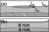
-
a.
Which phase has the higher interface tension against the container wall? Hint: look at the contact angle at the container wall.
-
b.
Write down the force balance for the three phase contact line for partial wetting and express the interface energies of A and B against the vapor phase by the contact angles and the interface tension \(\gamma _{\mathrm{{AB}}}\) of the A-rich phase versus the B-rich phase.
-
a.
-
2.
Assume that the binodal \(T_{\mathrm{{bin}}}(\phi )\) of an A and B mixture is characterized by the equation
$$\begin{aligned} \frac{T_{\mathrm{{bin}}}(\phi )}{\text{ K }}=1600\phi ^2-1600 \end{aligned}$$-
a.
Determine the critical point.
-
b.
A mixture 20 mL of A and 40 mL of B is prepared at the temperature 300 K. Is the mixture in a one phase state, or in a two phase state?
-
c.
Determine the compositions of the two phases.
-
d.
Determine the volumes of the two phases.
-
a.
-
3.
Consider a blend of polystyrene PS (C\(_8\)H\(_8\), \(\rho =1.04\,\text{ g/cm }^3\)) of molecular mass \(M_w=25\,000\,\text{ g/mol }\) and polyisoprene PI (C\(_5\)H\(_8\), \(\rho =0.93\,\text{ g/cm }^3\)) of molecular mass \(M_w=20\,000\,\text{ g/mol }\). Use the polystyrene monomer volume as cell volume \(v_c\).
-
a.
Determine the degrees of polymerization \(N_{\mathrm{{PS}}}\) and \(N^{\prime }_{\mathrm{{PI}}}\), and the effective degree of polymerization for \(N_{\mathrm{{PI}}}\) to be used in a Flory-Huggins description.
-
b.
For an interaction parameter \(\chi =0.1\), do you expect a mixed (one phase) or a de-mixed (two phase) state at the temperature \(T=150\,^{\circ }\text{ C }\)?
-
a.
-
4.
Derive (8.36).
-
5.
Linear response theory: start from the quadratic approximation (8.23) for \(\varDelta \omega _{\mathrm{{mix}}}\) and consider the effect of an external field h by an additional linear term \(h\phi \). Determine the new equilibrium position \(\phi _{\mathrm{{eq}}}(h)=\phi _{\mathrm{{eq}}}+\varDelta \phi \) with h and show that the response \(\varDelta \phi =\phi _{\mathrm{{eq}}}(h)-\phi _{\mathrm{{eq}}}(h=0)\) is linear in h. Determine the response coefficient \(\frac{\mathrm{d}\phi _{\mathrm{{eq}}}}{ \text{ d }h}\).
- 6.

8 Appendix
8.1 Calculus of Variations
A brief summary of functionals and their derivatives clearly remains insufficient from a mathematical point of view. However, it provides the techniques to perform the calculus of variations employed in this contribution. We follow the presentation of Großmann, and recommend his book for a detailed discussion on solid mathematical grounds [28].
Starting point is a space \(\mathscr {F}\) of functions \(f:\mathscr {M}\mapsto \mathbb {R}\), which can be chosen with sufficiently tame properties. Here \(\mathscr {M}\subset \mathbb {R}^n\) is the space of arguments for the functions, for our purposes the real axis \(\mathscr {M}=\mathbb {R}\), the 3D space \(\mathscr {M}=\mathbb {R}^3\) for bulk problems, or \(\mathscr {M}=\mathbb {R}^2\times \mathbb {R}_+\) for interface problems. The latter describes the half space with only non-negative z values. The tame functions \(f,g\in \mathscr {F}\) are assumed to be steady and sufficiently often differentiable. For two functions \(f,g\in \mathscr {F}\) the integration of the product fg over \(\mathscr {M}\) is considered as scalar product \(\left\langle f|g\right\rangle \) over \(\mathscr {F}\). A functional
maps \(\mathscr {F}\) to the real numbers \(\mathbb {R}\) and assigns to each \(f\in {\mathscr {F}}\) a real number r.
As a first example, a fixed function \(g\in {\mathscr {F}}\) can be chosen, which forms the kernel in an integral
So, \(f(\mathbf {x})\) is mapped by the functional F to the real number calculated as the integral over the product \(g(\mathbf {x})f(\mathbf {x})\), so the scalar product mentioned above. The squared brakets of F[.] which were used in (8.3), (8.7), (8.43), and (8.51) indicate the dependence of the functional F on the function f. A more general functional can take also derivatives of f(x) into account, and the squared gradient theories in the form (8.3) are examples for such functionals. A second example to assign a real value to a function f(x) defined over an interval \(\mathscr {I}\) is to select a specific point \(x_0\in \mathscr {I}\) and to evaluate \(f(x_0)\). Formally, the corresponding functional \(\delta _{x_0}[f]=f(x_0)\) can be written in a similar form as in (8.115):
The kernel \(\delta (x-x_0)\) of \(\delta _{x_0}[.]\) is usually called a delta function, although it cannot be defined in a mathematically consistent way as a function. The interpretation of (8.116) as a formal notation for the functional which assigns to each \(f\in \mathscr {F}\) its value \(f(x_0)\) gives a more consistent picture. The concept of a distribution which forms the basis for \(\delta (x-x_0)\) is also discussed by Großmann [28].
The calculation of an equilibrium interface profile is traced back to a minimization of a functional (8.43) which yields the interfacial energy for arbitrary interfacial profiles. Similar to a discussion of the minimum of a function, the minimum is found by setting the derivative equal to zero. However, now we have to use a functional derivative, not the normal derivative. The derivative of the functional F at the ‘position’ \(f\in \mathscr {F}\) in the ‘direction’ \(h\in \mathscr {F}\) is calculated as:
Under suitable conditions for a steady behavior of \(\frac{\partial F}{\partial f}[h]\) in f and h, the existence of functional derivations in specific directions (8.117) implies the existence of a unique functional derivative
The resulting functional derivative \(\frac{\delta F}{\delta f}\) is again a functional in h. It can be written as an integral over the kernel \(\frac{\delta F}{\delta f(x)}\), which might be either a regular integration, as in (8.115), or a formal integral similar to (8.116). While F[h] might contain also derivatives of h, they can be removed by partial integration in order to reach the representation of \(\frac{\delta F}{\delta f}[.]\) as an integral which contains h only and no derivatives of h. In this way, it can be expressed as a scalar product in the second form of (8.118). Removing any derivative of h is important when the first functional derivative is set equal to zero in order to find a function with an extremal value. For the mathematically sloppy discussion we are bound to in this brief appendix, we can assume the existence of the functional derivative \(\frac{\delta F}{\delta f}\) of (8.118), if the limit in (8.117) leads to an expression which is linear in h, so a presentation as scalar product in (8.118) is possible with a kernel \(\frac{\delta F}{\delta f(x)}\) independent of h.
A well known example in physics is the functional derivative of the action
of the differentiable trace x(t) with speed \(\dot{x}=\frac{\mathrm{d}x}{\mathrm{d}t}\) of a particle which starts at time \(t_1\) and ends at time \(t_2\). Here, L(x, v, t) is a two times differentiable Lagrange-function. For the potential energy V(x) it reads \(L(x,v,t)=\frac{1}{2}mv^2-V(x)\). The functional derivative in the ‘direction’ h(t) is now calculated according to (8.117) as
The arguments of the Lagrange-function \(L(x(t),\dot{x}(t),t)\) are not written explicitly in (8.120) and will also be omitted in the following equations, for facility of inspection. The time derivative \(\dot{h}(t)\) can be removed by integration by parts, which leads to the form
Since (8.121) is linear in h, the functional derivative in the direction h, \(\frac{\partial F}{\partial x}\), represents the functional derivative \(\frac{\delta F}{\delta x}\), which does not depend on the choice of h. Its kernel can be extracted from the integral of (8.121) and reads
The test function h(t) describes the variation of the path x(t), see (8.117). For fixed starting and end points of a path only variations with \(h(t_1)=h(t_2)=0\) are considered, and the boundary terms in (8.122) indicated by the delta functions do not contribute. For a path of extremal action, the functional derivative (8.121) needs to vanish for any such variation h. Thus, the kernel (8.122) needs to vanish, and we arrive at the Euler-Lagrange equation
Inserting the arguments of \(L(x(t),\dot{x}(t),t)\) into (8.123) leads to a differential equation, the solution of which is the path of the particle.
A second example adapted to interface problems starts from the functional
While x and y range from \(-\infty \) to \(+\infty \), z extends only from 0 which is the location of the interface to \(+\infty \). The Lagrange function is extracted from (8.124):
We consider only variations h which vanish for \(x,y\rightarrow \pm \infty \) and \(z\rightarrow +\infty \). A calculation similar to (8.120) leads to the kernel of \(\frac{\delta F}{\delta \phi }\):
Since the squared gradients in x and y in (8.124) give positive contributions, they need to vanish for the equilibrium interface profile. So (8.124) and (8.126) effectively depend on the gradient in z direction only and thus the problem becomes a one dimensional. Apart from the contact potential, (8.124) corresponds to (8.51), and (8.126) is similar to (8.52). Also bulk fluctuations are described by (8.126), if the kernel is integrated over the full \(\mathbb {R}^3\). The boundary term at the interface with \(\delta (z)\) vanishes, if we consider variations with \(h(z)=0\), so for a profile with fixed value at the interface. When \(\phi (z=0)\) is not fixed but determined by an interface potential, the gradient in the boundary term affects the boundary condition for fluctuation modes in the second functional derivative.
For the calculation of the second functional derivative \(\frac{\delta ^2 F}{\delta f^2}\), one considers the first derivative \(\frac{\delta F}{\delta f}[h]\) as a functional in f for fixed ‘direction’ h. For this functional in f, the functional derivative is calculated with the same rules. The second derivative can be written either as an integral, or as a bi-linear mapping, similar to the scalar product (8.115):
We do not look for an extremum with the second derivative, and so we do not set the kernel (8.127) equal to zero, as we did in (8.123). So, it is not required and often not possible to remove the derivatives of k by partial integration, and thus \(\frac{\delta ^2 F}{\delta ^2 f(x)}\) might contain derivative operators acting on k. In case the derivative of a product of a term included in \(\frac{\delta ^2 F}{\delta ^2 f(x)}\) and k(x) is encountered, it can be resolved with the product rule of derivation for improved clarity. A function f which results in an extremum as determined by the first functional derivative and its derivative can be inserted to the Lagrange Function of (8.127), in order to build up a bi-linear form for fluctuations around the equilibrium profile. This bi-linear form allows the definition of orthogonality of fluctuation modes. Eigen-fluctuations are the eigen-modes of the bi-linear form, and if these eigen-fluctuations have different eigen-values they are necessarily orthogonal. Higher derivatives can be calculated along the same lines, and a Taylor expansion for a functional reads
As an illustration of the second derivative, we use the second example (8.124), start from the first derivative (8.118) with (8.126) inserted, and perform a limit calculation with a second variation with respect to k(t) similar to (8.120). The kernel operator of the resulting bilinear form (8.127) results as
8.2 List of Important Symbols
Symbol | First Occurrence | Meaning |
|---|---|---|
\(\tilde{A}\) | (8.27) | scattering amplitude |
\(\alpha \) | (8.19) | length ratio of the polymers of a blend |
\(\chi \) | (8.13) | Flory-Huggins interaction parameter |
F, \(\varDelta F\), \(\varDelta f\) | free energy, free energy increment and its density | |
\(\varDelta F_{{\mathrm{{mix}}}}\), \(\varDelta f_{\mathrm{{mix}}}\) | Free energy of mixing and its density, Flory-Huggins theory | |
\(\varDelta f_{\mathrm{{L}}}\) | (8.61) | free energy density Landau theory |
\(\varDelta \varOmega \), \(\varDelta \omega _{\mathrm{{mix}}}\) | grand canonical potential increment and its density | |
\(\varDelta \omega _{ \mathrm{{L}}}\), \(\varDelta \omega _{\mathrm{{L,red}}}\) | density grand canonical potential Landau theory, reduced form | |
\(\varDelta \omega _{\mathrm{{bulk}}}\), \(\varDelta \omega _{\mathrm{{bulk,red}}}\) | minimum density grand canonical potential, reduced form | |
\(\phi \), \(\phi '\), \(\phi ''\) | volume fraction of B, deviation from \(\phi _{\mathrm{{c}}}\), deviation from \(\phi _{\mathrm{{eq}}}\) | |
\(\phi _{\mathrm{{a}}}\), \(\phi _{\mathrm{{b}}}\) | (8.20) | compositions on the A-rich and B-rich side on the binodal line |
\(\phi _0\), \(\phi _{0\mathrm{{a}}}\), \(\phi _{0\mathrm{{b}}}\) | contact compositions at a substrate, for A-rich and B-rich phases | |
\(\phi _{\mathrm{{c}}}\) | (8.59) | critical composition |
\(\bar{\phi }\) | average composition set by sample preparation | |
\(\phi _{\mathrm{{eq}}}\) | (8.23) | equilibrium composition |
\(\phi _{\mathrm{{pw}}}\) | (8.78) | bulk composition at the start of the pre-wetting line |
\(\phi _{\mathrm{{red}}}\), \(\phi _{\mathrm{{red,0}}}\) | reduced composition, contact value of it | |
\(\phi _{\mathrm{{red,0,P}}}\), \(\phi _{\mathrm{{red,0,Q}}}\) | reduced contact composition on the P line and the Q line | |
\(\phi _{\mathrm{{w}}}\) | Fig. 8.7 | bulk composition at the wetting transition |
\(\kappa \) | (8.3) | elastic constant of a squared gradient theory |
\(\mu _{\mathrm{{A}}}\), \(\mu _{\mathrm{{B}}}\) | (8.21) | chemical potential of A polymers and B polymers |
\(N_{\mathrm{{A}}}\), \(N_{\mathrm{{B}}}\), \(N_{\mathrm{{B}}}'\) | (8.11) | degree of polymerization of the A and of the B molecules |
\(n_{\mathrm{{A}}}\), \(n_{\mathrm{{B}}}\) | (8.11) | number of A polymers and number of B polymers in the volume |
\(R_{\mathrm{{g}}}\), \(R_{\mathrm{{gA}}}\), \(R_{\mathrm{{gB}}}\) | (8.37) | radius of gyration, for A and B chains |
\(S_{\mathrm{{a}}}\) | (8.2) | spreading coefficient of the A-rich phase |
\(\gamma _{\mathrm{{ab}}}\) | (8.1) | interface tension between the A-rich phase and the B-rich phase |
\(\gamma _{\mathrm{{AS}}}\), \(\gamma _{\mathrm{{BS}}}\) | (8.50) | interface tensions between the pure A phase or the pure B phase and a substrate |
\(\gamma _{\mathrm{{aS}}}\), \(\gamma _{\mathrm{{bS}}}\) | (8.1) | interface tensions between the A-rich phase or the B-rich phase and a substrate |
\(\gamma _{\mathrm{{S}}}(\phi )\) | (8.50) | contact potential at a substrate |
\(T_{\mathrm{{bin}}}\), \(T_{\mathrm{{spin}}}\) | binodal and spinodal temperature | |
\(\varTheta _{\mathrm{{a}}}\) | (8.1) | contact angle of the A-rich phase |
\(T_{\mathrm{{pw}}}\) | temperatures at the start of the pre-wetting line | |
\(T_{\mathrm{{w}}}\) | bulk composition at the wetting transition | |
\(T_{\mathrm{{c}}}\) | (8.64) | temperature of the bulk critical point |
\(V_{\mathrm{{A}}}\), \(V_{\mathrm{{B}}}\) | (8.11) | total volumes of A and B |
\(v_{\mathrm{{A}}}\), \(v_{\mathrm{{B}}}\) | (8.11) | volumes of an A monomer and a B monomer |
\(v_{\mathrm{{c}}}\) | (8.11) | cell volume in the Flory-Huggins theory |
\(\xi \), \(\xi _{\mathrm{{bin}}}\) | correlation length of fluctuations, \(\xi \) on the binodal line | |
\(z_{\mathrm{{eff}}}\) | (8.11) | number of neighboring cells in the Flory-Huggins theory |
Notes
- 1.
Strobl uses in his book the term free enthalpy instead of free energy, which is employed here. In order to describe experiments theoretically, the free enthalpy would be more appropriate, since experiments are in most cases performed at constant pressure, not at constant volume. However, the Flory-Huggins theory contains the volume V as explicit parameter, not the pressure P. Therefore, it is formally a free energy, not a free enthalpy. Since the volume change of polymer blends upon mixing or heating is usually negligible, there is basically no difference between the free energy and the free enthalpy.
- 2.
The formal difference between the total free energy density in (8.3) and the free energy increment to a constant background is of minor importance, as any calculation is based on derivatives of the free energy, where any constant shift of the energy scale cancels out.
- 3.
For a finite scattering volume the fluctuations form a Fourier series, not a Fourier integral transformation.
- 4.
For data gained from a real experiment, the measured intensity needs to be corrected by subtracting the background scattering of the solvent.
- 5.
- 6.
An excellent discussion of thermal excitation and time correlation function as described by a Langevin equation is found in the book of Doi and Edwards [19].
- 7.
In this step, a \(\phi \) dependence of the elastic constant \(\kappa \) would lead to an additional term, which does not fit to the following manipulations in a simple way.
- 8.
For a neutral substrate with \(\gamma _{\mathrm{{AS}}}=\gamma _{\mathrm{{BS}}}\) and thus no preferential adsorption, the substrate would have no effect on the sample. This boring case does not need further discussion.
- 9.
The delta function is also briefly discussed in the appendix.
- 10.
- 11.
The mechanism of such a continuous transition is different from the discussion of Bonn and Ross [4]. They investigate conditions for the contact composition which could lead to a continuous transition based on a graphical method eqivalent to (8.55) with an additional, \(\phi \) dependent term on the right side. Based on a discussion of this slope of the right side, they identify conditions for the contact composition where the wetting transition becomes continuous. They find continuous transitions at a higher temperature than \(T_{\mathrm{{pw}}}\). In the discussion here, in contrast, the reason for continuous wetting is a calculated value \(|\cos (\varTheta _{\mathrm{{a}}})|>1\) at \(T_{\mathrm{{pw}}}\), which leads to continuous wetting at lower temperature than \(T_{\mathrm{{pw}}}\). The discussion of Bonn and Ross does not include a test of the magnitude of \(|\cos (\varTheta _{\mathrm{{a}}})|\) resulting from their derived boundary values.
- 12.
Due to the linearity of (8.59), \(\phi '\) can simply replace \(\phi \) in all derivatives, e.g. \(\frac{\mathrm{{d}}\phi }{{\mathrm{d}}z}=\frac{\mathrm{{d}}\phi '}{{\mathrm{d}}z}\) or \(\frac{\mathrm{{d}}\omega }{{\mathrm{d}}\phi }=\frac{\mathrm{{d}}\omega }{{\mathrm{d}}\phi '}\). In order to apply the equations in Sect. 8.5.1 with \(\phi '\) instead of \(\phi \), one could write (8.43) with a new function \(\tilde{\omega }(\phi ')=\omega (\phi _{\mathrm{{c}}}+\phi ')\), and repeat all derivations of Sect. 8.5.1 with \(\tilde{\omega }(\phi ')\) instead of \(\omega (\phi )\). In order to keep the notation traceable, we use the same symbol and write sloppily \(\omega (\phi ')\) for \(\tilde{\omega }(\phi ')\).
- 13.
For a quick and dirty check, one can plot (8.93) with example values \(\phi _{\mathrm{{a}}}'=-1\), \(\phi _{\mathrm{{b}}}'=+1\), and \(\phi _0''=-1\).
- 14.
For the integration of the profile, use a partial fraction decomposition of (8.103)
$$\begin{aligned} \frac{2(\vartheta +1)Z_{\mathrm{{red}}}}{Z_{\mathrm{{red}}}^2-Z_{\mathrm{{red}}}-\vartheta /4}=\frac{\sqrt{\vartheta +1}(1+\sqrt{\vartheta +1})}{Z_{\mathrm{{red}}}-\frac{1}{2}-\frac{1}{2}\sqrt{\vartheta +1}}-\frac{\sqrt{\vartheta +1}(1-\sqrt{\vartheta +1})}{Z_{\mathrm{{red}}}-\frac{1}{2}+\frac{1}{2}\sqrt{\vartheta +1}}{.} \end{aligned}$$.
References
R. Sigel, Curr. Opin. Colloid Interface Sci. 14, 426–437 (2009)
E.H.A. de Hoog, H.N.W. Lekkerkerker, Measurement of the interfacial tension of a phase-separated colloid-polymer suspension. J. Phys. Chem. B 103, 5274–5279 (1999)
J.N. Israelachvili, Intermolecular and Surface Forces (Academic Press, Orlando, 2010)
D. Bonn, D. Ross, Wetting transitions. Rep. Prog. Phys. 64, 1085–1163 (2001)
G. Strobl, The Physics of Polymers (Springer, New York, 1996)
J.W. Cahn, Critial point wetting. J. Chem. Phys. 31, 3667–3672 (1977)
R.A.L. Jones, R.W. Richards, Polymers at Surfaces and Interfaces (Cambridge University Press, Cambridge, 1999)
A. Erbe, K. Tauer, R. Sigel, Ion distribution around electrostatic stabilized poly(styrene) latex particles studied by ellipsometric light scattering. Langmuir 23, 452–459 (2007)
R. Okamoto, A. Onuki, Charged colloids in an aqueous mixture with a salt. Phys. Rev. E 84, 051401 (2011)
J.W. Cahn, J.E. Hilliard, Free energy of a nonuniform system. I. Interfacial free energy. J. Chem. Phys. 28, 258–267 (1958)
J. Cahn, Free energy of a nonuniform system. II. Thermodynamic basis. J. Chem. Phys. 30, 1121–1124 (1959)
J.W. Cahn, J.E. Hilliard, Free energy of a nonuniform system. III. Nucleation in a two component incompressible fluid. J. Chem. Phys. 31, 688–699 (1959)
A.G. Lamorgese, D. Molin, R. Mauri, Phase field approach to multiphase flow modeling. Milan J. Math. 79, 597–642 (2011)
P. Sheng, E.B. Priestley, The Landau-de Gennes Theory of Liquid Crystal Phase Transitions, in Introduction to liquid crystals ed. by E.B. Priestley, P. Wojtowicz, P.J. Sheng (Plenum Press, New York, 1974), pp. 143–201
M.L. Huggins, Solutions of long chain compounds. J. Chem. Phys. 9, 440 (1941)
P.J. Flory, Thermodynamics of high polymer solutions. J. Chem. Phys. 9, 660–661 (1941)
J.S. Higgins, H.C. Benoitl, Polymers and Neutron Scattering (Clarendon Press, Oxford, 2002)
S. Dattagupta, Relaxation Phenomena in Condensed Matter Physics (Academic Press, Orlando, 1987)
M. Doi, S.F. Edwards, The Theory of Polymer Dynamics (Clarendon, Oxford, 1988)
P. Sheng, Boundary layer phase transitions in liquid crystals. Phys. Rev. A 26, 1610–1617 (1982)
E.F. Gramsbergen, L. Longa, W.H. de Jeu, Landau theory of the nematic-isotropic phase transition. Phys. Rep. 135, 196–257 (1986)
J.C. Tarczon, K. Miyano, Surface induced ordering of a liquid crystal in the isotropic phase. II. 4methoxybenzylidene-4-n-butylaniline (MBBA). J. Chem. Phys. 73, 1994–1998 (1980)
G. Grosche, V. Ziegler, D. Ziegler, Bronstein-Semendjajew: Taschenbuch der Mathematik (Verlag Harri Deutsch, Thun, 1985)
W.H. Press, S.A. Teukolsky, W.T. Vetterling, B.,P. Flannery, Numerical Recipes Third Edition (Cambridge University Press, Cambridge, 2007)
R. Sigel, Untersuchung der nematischen Randschicht eines isotropen Flüssigkristalls mit evaneszenter Lichtstreuung. PhD thesis, Freiburg (1997)
R. Sigel, G. Strobl, Light scattering by fluctuations within the nematic wetting layer in the isotropic phase of a liquid crystal. J. Chem. Phys. 112, 1029–1039 (2000)
R. Sigel, G. Strobl, Static and dynamic light scattering from the nematic wetting layer in an isotropic liquid crystal. Prog. Coll. Polym. Sci. 104, 187–190 (1997)
S. Großmann, Funktionalanalysis, 4th edn. (AULA-Verlag Wiesbaden, 1988)
Acknowledgments
The author thanks Helgard Sigel for her hospitality during summer 2014 in Markdorf, when the first part of this contribution was written.
Author information
Authors and Affiliations
Corresponding author
Editor information
Editors and Affiliations
Rights and permissions
Copyright information
© 2016 Springer International Publishing Switzerland
About this chapter
Cite this chapter
Sigel, R. (2016). Interfaces of Binary Mixtures. In: Lang, P., Liu, Y. (eds) Soft Matter at Aqueous Interfaces. Lecture Notes in Physics, vol 917. Springer, Cham. https://doi.org/10.1007/978-3-319-24502-7_8
Download citation
DOI: https://doi.org/10.1007/978-3-319-24502-7_8
Published:
Publisher Name: Springer, Cham
Print ISBN: 978-3-319-24500-3
Online ISBN: 978-3-319-24502-7
eBook Packages: Physics and AstronomyPhysics and Astronomy (R0)