Data Quality Dimensions

Abstract

In Chap. 1, we provided an intuitive concept of information quality and we informally introduced several data quality dimensions, such as accuracy, completeness, currency, and consistency.

These keywords were added by machine and not by the authors. This process is experimental and the keywords may be updated as the learning algorithm improves.

2.1 Introduction

In Chap. 1, we provided an intuitive concept of information quality and we informally introduced several data quality dimensions, such as accuracy , completeness, currency, and consistency .

This chapter investigates information quality in greater depth, in particular with reference to structured data, typical of relational databases, and presents multiple associated dimensions. Due to this focus, in this chapter we will adopt the term data quality and the acronym DQ for it. Each dimension captures a specific aspect included under the general umbrella of data quality. Both data and schema dimensions are important. Data of low quality deeply influence the quality of business processes, while a schema of low quality, e.g., an unnormalized schema in the relational model, results in potential redundancies and anomalies during the life cycle of data usage. Data dimensions can be considered more relevant in real-life applications and processes than schema dimensions.

More specifically, quality dimensions can refer either to the extension of data, i.e., to data values, or to their intension, i.e., to their schema. Both data dimensions and schema dimensions are usually defined in a qualitative way, referring to general properties of data and schemas, and the related definitions do not provide any facility for assigning values to dimensions themselves. Specifically, definitions do not provide quantitative measures, and one or more metrics are to be associated with dimensions as separate, distinct properties. For each metric, one or more measurement methods are to be provided regarding (see [521]) (1) where the measurement is taken, (2) what data are included, (3) the measurement device, and (4) the scale on which results are reported. Based on the literature, at times we will distinguish between dimensions and metrics, while at other times we will directly provide metrics.

The quality of conceptual and logical schemas is very important in database design and usage. Conceptual schemas are typically produced within the first phase of the development of an information system (IS). Erroneous conceptual schema design strongly impacts the system development and must be detected as soon as possible. Logical schemas are at the base of the implementation of any database application. Methods and techniques for assessing, evaluating, and improving conceptual schemas and logical schemas in different application domains is still a fertile research area.

Despite such recognized importance, the prevalent attention to the definitions of DQ dimensions has been devoted to data values, which are used, more extensively than schemas, in business and administrative processes. As a consequence, in this chapter we deal especially with data dimensions, but we also discuss some of the most relevant schema dimensions.

In the following sections, we describe in detail data dimensions in order to understand the different possible meanings and metrics. As a terminological note, when we refer to the relational model, we use the term tuple to indicate a set of fields or cell values , corresponding usually to different definition domains or domains, describing properties or attributes of a specific real-world object; we use interchangeably the terms relational table or table or relation to indicate a set of tuples. When we refer to generic data, we use the term record to indicate a set of fields, and we use interchangeably the terms file or dataset to indicate a set of tuples. As a consequence, tuple can be used in place of record and table∕relation can be used in place of structured file .

The chapter is organized as follows. In Sect. 2.2, we introduce a classification framework of data and information quality dimensions grouped in clusters of “similar” dimensions. In Sects. 2.3–2.6, we focus on specific clusters, namely, accuracy, completeness, accessibility, and consistency.

Some proposals of comprehensive classifications of dimensions are first illustrated and then compared in Sect. 2.7. Section 2.8 deals with schema dimensions, briefly describing correctness , minimality, completeness, and pertinence and, in more detail, readability and normalization.

2.2 A Classification Framework for Data and Information Quality Dimensions

Dimensions for data quality introduced in this chapter and dimensions for information quality discussed in subsequent chapters of the book can be characterized by a common classification framework that allows us to compare dimensions across different information types. The framework is based on a classification in clusters of dimensions proposed in [45] where dimensions are included in the same cluster according to their similarity. Clusters are defined in the following list, where the first item in italics is the representative dimension of the cluster, followed by other member dimensions. In this section, dimensions will be introduced informally and their meaning will be left to intuition:

• 1. Accuracy, correctness, validity, and precision focus on the adherence to a given reality of interest.

• 2. Completeness , pertinence, and relevance refer to the capability of representing all and only the relevant aspects of the reality of interest.

• 3. Redundancy, minimality, compactness, and conciseness refer to the capability of representing the aspects of the reality of interest with the minimal use of informative resources.

• 4. Readability, comprehensibility, clarity , and simplicity refer to ease of understanding and fruition of information by users.

• 5. Accessibility and availability are related to the ability of the user to access information from his or her culture, physical status/functions, and technologies available.

• 6. Consistency, cohesion, and coherence refer to the capability of the information to comply without contradictions to all properties of the reality of interest, as specified in terms of integrity constraints, data edits, business rules, and other formalisms.

• 7. Usefulness, related to the advantage the user gains from the use of information.

• 8. Trust , including believability , reliability , and reputation, catching how much information derives from an authoritative source. The trust cluster encompasses also issues related to security.

The first six clusters will be considered in this chapter and in Chaps. 3–5. The usefulness cluster will be considered for images (Chap. 5) and for information in general in Chap. 11. The trust cluster will be discussed in Chap. 14 dedicated to Web data and Big Data.

In the following part of the book, dimensions will be introduced and discussed based on the above classification.

2.3 Accuracy Cluster

Accuracy is defined as the closeness between a data value v and a data value v′, considered as the correct representation of the real-life phenomenon that the data value v aims to represent. As an example if the name of a person is John, the value v′ = John is correct, while the value v = Jhn is incorrect.

The world around us changes, and what we have called in the above definition “the real-life phenomenon that the data value v aims to represent” reflects such changes. So, there is a particular yet relevant type of data accuracy that refers to the rapidity with which the change in real-world phenomenon is reflected in the update of the data value; we call temporal accuracy such type of accuracy, in contrast to structural accuracy (or, simply, accuracy), that characterizes the accuracy of data as observed in a specific time frame, where the data value can be considered as stable and unchanged. In the following, we will consider first structural accuracy and later temporal accuracy.

2.3.1 Structural Accuracy Dimensions

Two kinds of (structural) accuracy can be identified, namely, a syntactic accuracy and a semantic accuracy.

Syntactic accuracy is the closeness of a value v to the elements of the corresponding definition domain D. In syntactic accuracy, we are not interested in comparing v with the true value v′; rather, we are interested in checking whether v is any one of the values in D, whatever it is. So, if v = Jack, even if v′ = John, v is considered syntactically correct, as Jack is an admissible value in the domain of persons’ names. Syntactic accuracy is measured by means of functions, called comparison functions , that evaluate the distance between v and the values in D. Edit distance is a simple example of a comparison function, taking into account the minimum number of character insertions, deletions, and replacements to convert a string s to a string s′. More complex comparison functions exist, for instance, taking into account similar sounds or character transpositions. In Chap. 8, a detailed description of the main comparison functions will be provided.

Let us consider the relation Movies introduced in Chap. 1, shown in Fig. 2.1.

Fig. 2.1

A relation Movies

The value Rman Holiday in movie 3 for Title is syntactically inaccurate, since it does not correspond to any title of a movie. Roman Holiday is the closest movie name to Rman Holiday; indeed, the edit distance between Rman Holiday and Roman Holiday is equal to 1 and simply corresponds to the insertion of the char o in the string Rman Holidays. Since 1 is the edit distance, the measure of syntactic accuracy is 1. More precisely, given a comparison function C, we may define a measure of syntactic accuracy of a value v with respect to a definition domain D, as the minimum value of C, when comparing v with all the values in D. Such a measure will be in the domain [$0,\ldots,n$], where n is the maximum possible value that the comparison function may have.

Semantic accuracy is the closeness of the value v to the true value v′. Let us consider again the relation Movies in Fig. 2.1. The exchange of directors’ names in tuples 1 and 2 is an example of a semantic accuracy error: indeed, for movie 1, a director named Curtiz would be admissible, and thus it is syntactically correct. Nevertheless, Curtiz is not the director of Casablanca; therefore a semantic accuracy error occurs.

The above examples clearly show the difference between syntactic and semantic accuracy. Note that while it is reasonable to measure syntactic accuracy using a distance function, semantic accuracy is measured better with a < yes, no > or a < correct, not correct > domain. Consequently, semantic accuracy coincides with the concept of correctness. In contrast with what happens for syntactic accuracy, in order to measure the semantic accuracy of a value v, the corresponding true value has to be known, or, else, it should be possible, considering additional knowledge, to deduce whether the value v is or is not the true value.

From the above arguments, it is clear that semantic accuracy is typically more complex to calculate than syntactic accuracy. When it is known a priori that the rate of errors is low and the errors result typically from typos, then syntactic accuracy tends to coincide with semantic accuracy, since typos produce values close to the true ones. As a result, semantic accuracy may be achieved by replacing an inaccurate value with the closest value in the definition domain, under the assumption that it is the true one.

In a more general context, a technique for checking semantic accuracy consists of looking for the same data in different data sources and finding the correct data by comparisons. This latter approach also requires the solution of the object identification problem, i.e., the problem of understanding whether two tuples refer to the same real-world entity or not; this problem will be discussed extensively in Chaps. 8 and 9. The main issues to be addressed for solving the object identification problem are:

• Identification: Tuples in one or several sources may not have unique identifiers, and thus they need to be put in correspondence by means of appropriate matching keys.

• Decision strategy: Once tuples are linked on the basis of a matching key, a decision must be made to state whether it corresponds to the same entity or not.

The accuracy discussed above is referred to a single value of a relation attribute. In practical cases, coarser accuracy definitions and metrics may be applied. As an example, it is possible to calculate the accuracy of an attribute called attribute (or column)accuracy , of a relation (relation accuracy), or of a whole database (database accuracy) .

When considering accuracy for sets of values instead of single values, a further notion of accuracy can be introduced, namely, duplication . Duplication occurs when a real-world entity is stored twice or more in a data source. Of course, if a primary key consistency check is performed when populating a relational table, a duplication problem does not occur, provided that the primary key assignment has been made with a reliable procedure. The duplication problem is more relevant for files or other data structures that do not allow the definition of key constraints. A typical cost of duplication is, for example, the additional mailing cost that enterprises pay for mailing customers, when customers are stored more than once in the their database. An indirect cost must be added to this direct cost, which consists of the loss of reputation of the enterprise in the eyes of its customers who may be bothered by having to receive the same material more than once.

For relation and database accuracy, for both syntactic and semantic accuracy, a ratio is typically calculated between accurate values and the total number of values. For instance, the accuracy of a relation can be measured as the ratio between the number of correct cell values and the total number of cells in the table. More complex metrics can be defined that consider comparison functions; for instance, as we said before, a typical process for syntactic accuracy evaluation is to match tuples from the source under examination with tuples of another source which is supposed to contain the same but correct tuples.

In such a process, accuracy errors on attribute values can be either those that do not affect the tuple matching or those that can stop the process itself, not allowing the matching. For instance, an accuracy error on an attribute SocialSecurityNumber (SSN) value can seriously affect the matching attempt; instead, given that SSNs are used for matching, an accuracy error on an attribute with a minor identification power, such as Age, cannot prevent the identification process from being carried out correctly. In the rest of this section, we illustrate a few metrics (see [222]) taking these aspects into account.

Let us consider a relational schema R consisting of K attributes and a relational table r consisting of N tuples. Let q _ij (i = 1… N, j = 1… K) be a Boolean variable defined to correspond to the cell values y _ij such that q _ij is equal to 0 if y _ij is syntactically accurate; otherwise it is equal to 1.

In order to identify whether or not accuracy errors affect a matching of a relational table r with a reference table r′ containing correct values, we introduce a further Boolean variable s _i equal to 0 if the tuple t _i matches a tuple in r′, otherwise equal to 1. We can introduce three metrics to distinguish the relative importance of value accuracy in the context of the tuple. The first two metrics have the purpose of giving a different importance to errors on attributes that have a higher identification power, in line with the above discussion.

The first metric is called weak accuracy error and is defined as

$$\displaystyle{\sum _{i=1}^{N}\frac{\beta ((q_{i} > 0)\bigwedge (s_{i} = 0))} {N},}$$

where β(. ) is a Boolean variable equal to 1 if the condition in parentheses is true, 0 otherwise, and $q_{i} =\sum _{ j=1}^{K}q_{ij}$. Such metric considers the case in which for a tuple t _i accuracy errors occur (q _i  > 0) but do not affect identification (s _i  = 0).

The second metric is called strong accuracy error and is defined as

$$\displaystyle{\sum _{i=1}^{N}\frac{\beta ((q_{i} > 0)\bigwedge (s_{i} = 1))} {N},}$$

where β(. ) and q _i have the same meaning as above. Such a metric considers the case in which accuracy errors occur (q _i  > 0) for a tuple t _i and actually do affect identification (s _i  = 1).

The third metric gives the percentage of accurate tuples matched with the reference table. It is expressed by the degree of syntactic accuracy of the relational instance r

$$\displaystyle{\sum _{i=1}^{N}\frac{\beta ((q_{i} = 0)\bigwedge (s_{i} = 0))} {N} }$$

by actually considering the fraction of accurate (q _i  = 0) matched (s _i  = 0) tuples.

2.3.2 Time-Related Accuracy Dimensions

A relevant aspect of data is their change and update in time. In Chap. 1 we provided a classification of types of data according to the temporal dimension, in terms of stable, long-term-changing, and frequently changing data. The principal time-related dimensions proposed for characterizing the above three types of data are currency , volatility, and timeliness.

Currency concerns how promptly data are updated with respect to changes occurring in the real world. As an example in Fig. 2.1, the attribute #Remakes of movie 4 has low currency because a remake of movie 4 has been done, but this information did not result in an increased value for the number of remakes. Similarly, if the residential address of a person is updated, i.e., it corresponds to the address where the person lives, then the currency is high.

Volatility characterizes the frequency with which data vary in time. For instance, stable data such as birth dates have volatility equal to 0, as they do not vary at all. Conversely, stock quotes, a kind of frequently changing data, have a high degree of volatility due to the fact that they remain valid for very short time intervals.

Timeliness expresses how current the data are for the task at hand. The timeliness dimension is motivated by the fact that it is possible to have current data that are actually useless because they are late for a specific usage. For instance, the timetable for university courses can be current by containing the most recent data, but it is not timely if it is available only after the start of the classes.

We now provide possible metrics of time-related dimensions. Currency can be typically measured with respect to last update metadata, which correspond to the last time the specific data were updated. For data types that change with a fixed frequency, last update metadata allow us to compute currency straightforwardly. Conversely, for data types whose change frequency can vary, one possibility is to calculate an average change frequency and perform the currency computation with respect to it, admitting errors. As an example, if a data source stores product names that are estimated to change every 5 years, then a product with its last update metadata reporting a date corresponding to 1 month before the observation time can be assumed to be current; in contrast, if the date reported is 10 years before the observation time, it is assumed to be not current.

Volatility is a dimension that inherently characterizes certain types of data. A metric for volatility is given by the length of time (or its inverse) that data remain valid.

Timeliness implies that data not only are current but are also in time for events that correspond to their usage. Therefore, a possible measurement consists of (1) a currency measurement and (2) a check that data are available before the planned usage time.

More complex metrics can be defined for time-related dimensions. As an example, we cite the metric defined in [31], in which the three dimensions currency, volatility, and timeliness are linked by defining timeliness as a function of currency and volatility. More specifically,

• 1. Currency is defined as

  $$\displaystyle{Currency = Age + (DeliveryTime - InputTime),}$$

  where Age measures how old the data unit is when received, DeliveryTime is the time the information product is delivered to the customer, and InputTime is the time the data unit is obtained. Therefore, currency is the sum of how old data are when received (Age), plus a second term that measures how long data have been in the information system, (DeliveryTime − InputTime).

• 2. Volatility is defined as the length of time data remains valid.

• 3. Timeliness is defined as

  $$\displaystyle{\max \left \{0,1 - \frac{currency} {volatility}\right \}.}$$

  Timeliness ranges from 0 to 1, where 0 means bad timeliness and 1 means good timeliness.

Observe that the relevance of currency depends on volatility: data that are highly volatile must be current, while currency is less important for data with low volatility.

2.4 Completeness Cluster

Completeness can be generically defined as “the extent to which data are of sufficient breadth, depth, and scope for the task at hand” [645]. In [504], three types of completeness are identified. Schema completeness is defined as the degree to which concepts and their properties are not missing from the schema. Column completeness is defined as a measure of the missing values for a specific property or column in a table. Population completeness evaluates missing values with respect to a reference population.

If focusing on a specific data model, a more precise characterization of completeness can be given. In the following we refer to the relational model.

2.4.1 Completeness of Relational Data

Intuitively, the completeness of a table characterizes the extent to which the table represents the corresponding real world. Completeness in the relational model can be characterized with respect to (1) the presence/absence and meaning of null values and (2) the validity of one of the two assumptions called open world assumption (OWA) and closed world assumption (CWA). We now introduce the two issues separately.

In a model with null values, the presence of a null value has the general meaning of a missing value, i.e., a value that exists in the real world but for some reason is not available. In order to characterize completeness, it is important to understand why the value is missing. Indeed, a value can be missing either because it exists but is unknown or because it does not exist at all or because it may exist but it is not actually known whether it exists or not. For a general discussion on the different types of null values, see [30]; here we describe the three types of null values, by means of an example.

Let us consider a Person relation with the attributes Name, Surname, BirthDate, and Email. The relation is shown in Fig. 2.2. For the tuples with Id equal to 2, 3, and 4, the Email value is NULL. Let us suppose that the person represented by tuple 2 has no e-mail: no incompleteness case occurs. If the person represented by tuple 3 has an e-mail, but its value is not known, then tuple 3 presents an incompleteness. Finally, if it is not known whether the person represented by tuple 4 has an e-mail or not, incompleteness may not be the case.

Fig. 2.2

The Person relation, with different null value meanings for the e-mail attribute

In logical models for databases, such as the relational model, there are two different assumptions on the completeness of data represented in a relational instance r. The CWA states that only the values actually present in a relational table r and no other values represent facts of the real world. In the OWA we can state neither the truth nor the falsity of facts not represented in the tuples of r.

From the four possible combinations emerging from (1) considering or not considering null values and (2) assuming OWA or CWA, we will focus on the following two most interesting cases:

• 1. Model without null values with OWA

• 2. Model with null values with CWA

In a model without null values with OWA, in order to characterize completeness, we need to introduce the concept of reference relation . Given the relation r, the reference relation of r, called ref(r), is the relation containing all the tuples that satisfy the relational schema of r, i.e., that represent objects of the real world that constitute the present true extension of the schema.

As an example, if Dept is a relation representing the employees of a given department and one specific employee of the department is not represented as a tuple of Dept, then the tuple corresponding to the missing employee is in ref(Dept), and ref(Dept) differs from Dept in exactly that tuple. In practical situations, the reference relations are rarely available. Instead their cardinality is much easier to get. There are also cases in which the reference relation is available but only periodically (e.g., when a census is performed).

On the basis of the reference relation, the completeness of a relation r is measured in a model without null values as the fraction of tuples actually represented in the relation r, namely, its size with respect to the total number of tuples in ref(r):

$$\displaystyle{C(r) = \frac{\vert r\vert } {\vert ref(r)\vert }.}$$

As an example, let us consider the citizens of Rome. Assume that, from the personal registry of Rome’s municipality, the overall number is six million. Let us suppose that a company stores data on Rome’s citizens for the purpose of its business; if the cardinality of the relation r storing the data is 5,400,000, then C(r) is equal to 0.9.

In the model with null values with CWA, specific definitions for completeness can be provided by considering the granularity of the model elements, i.e., value, tuple, attribute, and relations, as shown in Fig. 2.3. Specifically, it is possible to define:

• A value completeness, to capture the presence of null values for some fields of a tuple

• A tuple completeness, to characterize the completeness of a tuple with respect to the values of all its fields

• An attribute completeness, to measure the number of null values of a specific attribute in a relation

• A relation completeness, to capture the presence of null values in a whole relation

Fig. 2.3

Completeness of different elements in the relational model

As an example, in Fig. 2.4, a Student relation is shown. The tuple completeness evaluates the percentage of specified values in the tuple with respect to the total number of attributes of the tuple itself. Therefore, in the example, the tuple completeness is 1 for tuples 6754 and 8907, 0.8 for tuple 6587, 0.6 for tuple 0987, and so on. One way to see the tuple completeness is as a measure of the information content of the tuple, with respect to its maximum potential information content. With reference to this interpretation, we are implicitly assuming that all values of the tuple contribute equally to the total information content of the tuple. Of course, this may not be the case, as different applications can weight the attributes of a tuple differently.

Fig. 2.4

Student relation exemplifying the completeness of tuples, attributes, and relations

The attribute completeness evaluates the percentage of specified values in the column corresponding to the attribute with respect to the total number of values that should have been specified. In Fig. 2.4, let us consider an application calculating the average of the votes obtained by students. The absence of some values for the Vote attribute simply implies a deviation in the calculation of the average; therefore, a characterization of Vote completeness may be useful.

The relation completeness is relevant in all applications that need to evaluate the completeness of a whole relation and can admit the presence of null values on some attributes. Relation completeness measures how much information is represented in the relation by evaluating the content of the information actually available with respect to the maximum possible content, i.e., without null values. According to this interpretation, completeness of the relation Student in Fig. 2.4 is 53/60.

2.4.2 Completeness of Web Data

Data that are published in Web information systems can be characterized by evolution in time. While in the traditional paper-based media, information is published once and for all, Web information systems are characterized by information that is continuously published.

Let us consider the Web site of a university, where a list of courses given at that university in the current academic year is published. At a given moment, the list can be considered complete in the sense that it includes all the courses that have been officially approved. Nevertheless, it is also known that more courses will be added to the list, pending their approval. Therefore, there is the need to apprehend how the list will evolve in time with respect to completeness. The traditional completeness dimension provides only a static characterization of completeness. In order to consider the temporal dynamics of completeness, as needed in Web information systems, we introduce the notion of completability.

We consider a function C(t), defined as the value of completeness at the instant t, with t ∈ [t_pub, t_max], where t_pub is the initial instant of publication of data and t_max corresponds to the maximum time within which the series of the different scheduled updates will be completed. Starting from the function C(t), we can define the completability of the published data as

$$\displaystyle{\int _{t{\_}curr}^{t{\_}max}C(t),}$$

where t_curr is the time at which completability is evaluated and t_curr <  t_max.

Completability, as shown in Fig. 2.5, can be graphically depicted as an area Cb of a function that represents how completeness evolves between an instant t_curr of observation and t_max. Observe that the value corresponding to t_curr is indicated as c_curr; c_max is the value for completeness estimated for t_max. The value c_max is a real reachable limit that can be specified for the completeness of the series of elements; if this real limit does not exist, c_max is equal to 1. In Fig. 2.5, a reference area A is also shown, defined as

$$\displaystyle{(t{\_}max - t{\_}curr) {\ast}\frac{c{\_}max - c{\_}pub} {2},}$$

that, by comparison with Cb, allows us to define ranges [High, Medium, Low] for completability.

Fig. 2.5

A graphical representation of completability

With respect to the example above, considering the list of courses published on a university Web site, the completeness dimension gives information about the current degree of completeness; the completability information gives the information about how fast this degree will grow in time, i.e., how fast the list of courses will be completed. The interested reader can find further details in [498].

In Chap. 14, we will describe the impact that low quality resulting from temporal variability of Web data has on the object identification problem.

2.5 Accessibility Cluster

Publishing large amounts of data in Web sites is not a sufficient condition for its availability to everyone. In order to access it, a user needs to access a network, to understand the language to be used for navigating and querying the Web, and to perceive with his or her senses the information made available. Accessibility measures the ability of the user to access the data from his or her own culture, physical status/functions, and technologies available. We focus in the following on causes that can reduce physical or sensorial abilities and, consequently, can reduce accessibility, and we briefly outline corresponding guidelines to achieve accessibility. Among others, the World Wide Web Consortium [637] defines the individuals with disabilities as subjects that

• 1. May not be able to see, hear, move, or process some types of information easily or at all

• 2. May have difficulty reading or comprehending text

• 3. May not have to or be able to use a keyboard or mouse

• 4. May have a text-only screen, a small screen, or a slow Internet connection

• 5. May not speak or understand a natural language fluently

Several guidelines are provided by international and national bodies to govern the production of data, applications, services, and Web sites in order to guarantee accessibility. In the following, we describe some guidelines related to data provided by the World Wide Web Consortium in [637].

The first, and perhaps most important, guideline indicates provision of equivalent alternatives to auditory and visual content, called text equivalent content. In order for a text equivalent to make an image accessible, the text content can be presented to the user as synthesized speech, braille, and visually displayed text. Each of these three mechanisms uses a different sense, making the information accessible to groups affected by a variety of sensory and other disabilities. In order to be useful, the text must convey the same function or purpose as the image. For example, consider a text equivalent for a photographic image of the continent of Africa as seen from a satellite. If the purpose of the image is mostly that of decoration, then the text “Photo of Africa as seen from a satellite” might fulfill the necessary function. If the purpose of the photograph is to illustrate specific information about African geography, such as its organization and subdivision into states, then the text equivalent should convey that information with more articulate and informative text. If the photo has been designed to allow the user to select the image or part of it (e.g., by clicking on it) for information about Africa, equivalent text could be “Information about Africa,” with a list of items describing the parts that can be selected. Therefore, if the text conveys the same function or purpose for the user with a disability as the image does for other users, it can be considered a text equivalent.

Other guidelines suggest:

• Avoiding the use of color as the only means to express semantics, helping daltonic people appreciate the meaning of data

• Usage of clear natural language, by providing expansions of acronyms, improving readability, a frequent use of plain terms

• Designing a Web site that ensures device independence using features that enable activation of page elements via a variety of input devices

• Providing context and orientation information to help users understand complex pages or elements

Several countries have enacted specific laws to enforce accessibility in public and private Web sites and applications used by citizens and employees in order to provide them effective access and reduce the digital divide.

Chapter 14 will further discuss accessibility of Web data with a focus on system-dependent features, e.g., session identification problems, robot detection and filtering, etc.

2.6 Consistency Cluster

The consistency dimension captures the violation of semantic rules defined over (a set of) data items, where items can be tuples of relational tables or records in a file. With reference to relational theory, integrity constraints are an instantiation of such semantic rules. In statistics, data edits are another example of semantic rules that allow for the checking of consistency .

2.6.1 Integrity Constraints

The interested reader can find a detailed discussion on integrity constraints in the relational model in [30]. The purpose of this section is to summarize the main concepts, useful in introducing the reader to consistency -related topics.

Integrity constraints are properties that must be satisfied by all instances of a database schema. Although integrity constraints are typically defined on schemas, they can at the same time be checked on a specific instance of the schema that presently represents the extension of the database. Therefore, we may define integrity constraints for schemas, describing a schema quality dimension, and for instances, representing a data dimension. In this section, we will define them for instances, while in Sect. 2.8, we will define them for schemas.

It is possible to distinguish two main categories of integrity constraints, namely, intrarelation constraints and interrelation constraints .

Intrarelation integrity constraints can regard single attributes (also called domain constraints) or multiple attributes of a relation.

Let us consider an Employee relational schema, with the attributes Name, Surname, Age, WorkingYears, and Salary. An example of the domain constraint defined on the schema is “Age is included between 0 and 120.” An example of a multiple attribute integrity constraint is “If WorkingYears is less than 3, then Salary could not be more than 25.000 Euros per year.”

Interrelation integrity constraints involve attributes of more than one relation. As an example, consider the Movies relational instance in Fig. 2.1. Let us consider another relation, OscarAwards, specifying the Oscar awards won by each movie and including an attribute Year corresponding to the year when the award was assigned. An example of interrelation constraint states that “Year of the Movies relation must be equal to Year of OscarAwards.”

Among integrity constraints, the following main types of dependencies can be considered:

• Key dependency. This is the simplest type of dependency. Given a relational instance r, defined over a set of attributes, we say that for a subset K of the attributes, a key dependency holds in r, if no two rows of r have the same K-values. For instance, an attribute like SocialSecurityNumber can serve as a key in any relational instance of a relational schema Person. When key dependency constraints are enforced, no duplication will occur within the relation (see also Sect. 2.3 on duplication issues).

• Inclusion dependency. Inclusion dependency is a very common type of constraint and is also known as referential constraint . An inclusion dependency over a relational instance r states that some columns of r are contained in other columns of r or in the instances of another relational instance s. A foreign key constraint is an example of inclusion dependency, stating that the referring columns in one relation must be contained in the primary key columns of the referenced relation.

• Functional dependency. Given a relational instance r, let X and Y be two nonempty sets of attributes in r. r satisfies the functional dependency $\mathtt{X} \rightarrow \mathtt{Y}$, if the following holds for every pair of tuples t ₁ and t ₂ in r:

  $$\displaystyle{\text{If}\ \mathtt{t}_{1}.\mathtt{X} = \mathtt{t}_{2}.\mathtt{X},\ \text{then}\ \mathtt{t}_{1}.\mathtt{Y} = \mathtt{t}_{2}.\mathtt{Y},}$$

  where the notation t ₁.X means the projection of the tuple t ₁ onto the attributes in X. In Fig. 2.6, examples of relations respectively satisfying and violating a functional dependency $\mathtt{AB} \rightarrow \mathtt{C}$ are shown. In the figure, the relation r ₁ satisfies the functional dependency, as the first two tuples, having the same values for the attribute A and the attribute B, also have the same value for the attribute C. The relation r ₂ does not satisfy the functional dependency, since the first two tuples have a different C field.

  Fig. 2.6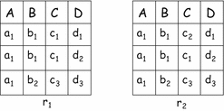

  

  Example of functional dependencies

2.6.2 Data Edits

In the previous section, integrity constraints were discussed within the relational model as a specific category of consistency semantic rules. However, where data are not relational, consistency rules can still be defined. As an example, in the statistical field, data coming from census questionnaires have a structure corresponding to the questionnaire schema. The semantic rules are thus defined over such a structure in a way very similar to relational constraints. Such rules, called edits, are less powerful than integrity constraints because they do not rely on a data model like the relational one. Nevertheless, data editing has been done extensively in the national statistical agencies since the 1950s and has revealed a fruitful and effective area of application. Data editing is defined as the task of detecting inconsistencies by formulating rules that must be respected by every correct set of answers. Such rules are expressed as edits, which denote error conditions.

As an example, an inconsistent answer to a questionnaire can be to declare

$$\displaystyle{\mathtt{marital\ status\ =\ \textquotedblright married\textquotedblright,\ age\ =\ \textquotedblright 5\ years\ old\textquotedblright }.}$$

The rule to detect this kind of errors could be the following:

$$\displaystyle\begin{array}{rcl} & & \mathtt{if\ marital\ status\ is\ married,\ age\ must\ not\ be} {}\\ & & \mathtt{less\ than\ 14}. {}\\ \end{array}$$

The rule can be put in the form of an edit, which expresses the error condition, namely,

$$\displaystyle{\mathtt{marital\ status\ =\ married}\ \wedge \ \mathtt{age} < 14.}$$

After the detection of erroneous records, the act of correcting erroneous fields by restoring correct values is called imputation . The problem of localizing errors by means of edits and imputing erroneous fields is known as the edit-imputation problem. In Chap. 7 we will examine some issues and methods for the edit-imputation problem.

2.7 Approaches to the Definition of Data Quality Dimensions

In this section we describe some general proposals for dimensions. There are three main approaches adopted for proposing comprehensive sets of the dimension definitions, namely, theoretical, empirical, and intuitive. The theoretical approach adopts a formal model in order to define or justify the dimensions. The empirical approach constructs the set of dimensions starting from experiments, interviews, and questionnaires. The intuitive approach simply defines dimensions according to common sense and practical experience.

In the following, we summarize three main proposals that clearly represent the approaches to dimension definitions: Wand and Wang [640], Wang and Strong [645], and Redman [519].

2.7.1 Theoretical Approach

A theoretical approach to the definition of data quality is proposed in Wand and Wang [640]. This approach considers an information system (IS) as a representation of a real-world system (RW); RW is properly represented in an IS if (1) there exists an exhaustive mapping $RW \rightarrow IS$ and (2) no two states in RW are mapped into the same state in the IS, i.e., the inverse mapping is a function (see Fig. 2.7).

Fig. 2.7

Proper representation of the real-world system in the theoretical approach from [640]

All deviations from proper representations generate deficiencies. They distinguish between design deficiencies and operation deficiencies . Design deficiencies are of three types: incomplete representation, ambiguous representation, and meaningless states. They are graphically represented in Fig. 2.8.

Fig. 2.8

(a) Incomplete, (b) ambiguous, and (c) meaningless representations of the real-world system in the theoretical approach

Only one type of operation deficiency is identified, in which a state in RW might be mapped to a wrong state in an IS; this is referred to as garbling. Garbling with a map to a meaningless state is dangerous, as it will preclude a map back to a real-world state (see Fig. 2.9a). Garbling to a meaningful but wrong state will allow the user to map back to a real-world state (see Fig. 2.9b).

Fig. 2.9

Garbling representations of the real-world system from [640]. (a) Not meaningful. (b) Meaningful

A set of data quality dimensions are defined by making references to described deficiencies. More specifically, the identified dimensions are (the quoted text is from [640]):

• Accuracy : “inaccuracy implies that the information system represents a real-world state different from the one that should have been represented.” Inaccuracy refers to a garbled mapping into a wrong state of the IS, where it is possible to infer a valid state of the real world though not the correct one (see Fig. 2.9b).

• Reliability indicates “whether the data can be counted on to convey the right information; it can be viewed as correctness of data.” No interpretation in terms of data deficiencies is given.

• Timeliness refers to “the delay between a change of the real-world state and the resulting modification of the information system state.” Lack of timeliness may lead to an IS state that reflects a past RW state.

• Completeness is “the ability of an information system to represent every meaningful state of the represented real-world system.” Completeness is of course tied to incomplete representations.

• Consistency of data values occurs if there is more than one state of the information system matching a state of the real-world system; therefore “inconsistency would mean that the representation mapping is one-to-many.” This is captured by the representation, so the inconsistency is not considered a result of a deficiency.

2.7.2 Empirical Approach

In the proposal discussed in Wang and Strong [645], data quality dimensions have been selected by interviewing data consumers. Starting from 179 data quality dimensions, the authors selected 15 different dimensions, represented in Fig. 2.10 with their definitions. A two-level classification is proposed, in which each of four categories is further specialized into a number of dimensions. The four categories are:

• Intrinsic data quality, capturing the quality that data has on its own. As an example, accuracy is a quality dimension that is intrinsic to data.

• Contextual data quality considers the context where data are used. As an example, the completeness dimension is strictly related to the context of the task.

• Representational data quality captures aspects related to the quality of data representation, e.g., interpretability.

• Accessibility data quality is related to the accessibility of data and to a further nonfunctional property of data access, namely, the level of security.

Fig. 2.10

Dimensions proposed in the empirical approach

2.7.3 Intuitive Approach

Redman [519] classifies DQ dimensions according to three categories, namely, conceptual schema, data values, and data format. Conceptual schema dimensions correspond to what we called schema dimensions. Data value dimensions refer specifically to values, independently of the internal representation of data; this last aspect is covered by data format dimensions. Our focus here is on data extension; therefore, in Fig. 2.11, we provide the definitions for data value and format dimensions only.

Fig. 2.11

Dimensions proposed in the intuitive approach [519]

2.7.4 A Comparative Analysis of the Dimension Definitions

According to the definitions described in the previous section, there is no general agreement either on which set of dimensions defines DQ or on the exact meaning of each dimension. In fact, in the illustrated proposals, dimensions are not defined in a measurable and formal way. Instead, they are defined by means of descriptive sentences in which the semantics are consequently disputable. Nevertheless, we attempt to make a comparison between the different definitions provided with the purpose of showing possible agreements and disagreements in the different proposals. In order to cover a larger number of proposals, besides those previously described by Wand and Wang [640], Wang and Strong [645], and Redman [519], we also consider Jarke et al. [341], Bovee et al. [86], Naumann [461], and Liu [408]. Hereafter we will refer to the proposals with the name of the first author of the work.

With regard to time-related dimensions , in Fig. 2.12, definitions for currency , volatility, and timeliness by different authors are illustrated. In the figure, Wand and Redman provide very similar definitions but for different dimensions, i.e., for timeliness and currency, respectively. Wang and Liu assume the same meaning for timeliness, Naumann proposes a very different definition for it, and Bovee only provides a definition for timeliness in terms of currency and volatility. Bovee’s currency corresponds to timeliness as defined by Wang and Liu. Volatility has a similar meaning in Bovee and Jarke. The comparison shows that there is no substantial agreement on the names to use for time-related dimensions; indeed, currency and timeliness are often used to refer to the same concept. There is not even agreement on the semantics of a specific dimension; indeed, for timeliness, different meanings are provided by different authors.

Fig. 2.12

Time-related dimension definitions

With regard to completeness , in Fig. 2.13, different proposals for completeness definitions are shown. By comparing such definitions, it emerges that there is substantial agreement on what completeness is, although it often refers to different granularity levels and different data model elements, e.g., information system in Wand, data warehouse in Jarke, and entity in Bovee.

Fig. 2.13

Completeness dimension definitions

2.7.5 Trade-Offs Between Dimensions

Data quality dimensions are not independent, i.e., correlations exist between them. If one dimension is considered more important than the others for a specific application, then the choice of favoring it may imply negative consequences for the other ones. In this section, we provide some examples of possible trade-offs.

First, trade-offs may need to be made between timeliness and any one of the three dimensions: accuracy, completeness, and consistency . Indeed, having accurate (or complete or consistent) data may need checks and activities that require time, and thus timeliness is negatively affected. Conversely, having timely data may cause lower accuracy (or completeness or consistency). A typical situation in which timeliness can be preferred to accuracy, completeness, or consistency is given by most Web applications: as the time constraints are often very stringent for Web data, it is possible that such data are deficient with respect to other quality dimensions. For instance, a list of courses published on a university Web site must be timely though there could be accuracy or consistency errors and some fields specifying courses could be missing. Conversely, when considering an administrative application, accuracy , consistency, and completeness requirements are more stringent than timeliness, and therefore delays are mostly admitted in dimensions other than timeliness.

Another significant case of trade-off is between consistency and completeness [33]. Here the question is “Is it better to have less but consistent data, i.e., poor completeness, or to have more but inconsistent data?” This choice is again very domain specific. As an example, statistical data analysis typically requires a significant and representative amount of data in order to perform the analysis; in this case, the approach is to favor completeness, tolerating inconsistencies or adopting techniques to solve them. Conversely, when considering the publication of a list of votes obtained by students as the result of an exam, it is more important to have a list of consistency checked votes than a complete one, possibly deferring the publication of the complete list.

2.8 Schema Quality Dimensions

In the previous sections, we provided an in-depth characterization of DQ dimensions. In this section, the focus is on schema quality dimensions. However, there is a strict relationship between quality of schemas and quality of data, as highlighted in the next example. Let us suppose we want to model residence addresses of people; in Fig. 2.14, there are two possibilities to model such a concept. Specifically, in Fig. 2.14a, the residence addresses are modeled as attributes of a relation Person, while in Fig. 2.14b, the residence addresses are modeled as a relation Address, with the fields Id, StreetPrefix, StreetName, Number, and City, and a relation ResidenceAddress storing the address at which the person lives. The solution in Fig. 2.14a has some problems. First, representing addresses as a single field creates ambiguity on the meaning of the different components; for instance, in tuple 3 of the Person relation, is 4 a civic number or the number of the avenue (it is actually part of the name of the square)? Second, the values of the attribute Address can also contain information that is not explicitly required to be represented (e.g., the floor number and zip code of tuples 1 and 2 of the Person relation). Third, as the Person relation is not normalized, a redundancy problem occurs and hence further errors on the Address attribute may be potentially introduced (see the same address values for tuples 1 and 2 of the Person relation). On the other hand, the solution in Fig. 2.14b is more complex. In real implementation there is often the need to manage trade-offs between the two modeling solutions.

Fig. 2.14

Two ways of modeling residence addresses

A comprehensive proposal on schema dimensions is described in the book of Redman [519] and includes six dimensions and 15 subdimensions referring to schema quality.

Here, we focus on dimensions related to the accuracy, completeness, redundancy, and readability clusters introduced in Sect. 8.5.3 In the definitions we are going to provide, we assume that the database schema is the result of the translation of a set of requirements, expressed usually in natural language, into a set of conceptual (or logical) structures, expressed in terms of a conceptual (or logical) database model.

2.8.1 Accuracy Cluster

Accuracy, or better correctness in this context, is of two types:

• 1. Correctness with respect to the model concerns the correct use of the constructs of the model in representing requirements. As an example, in the Entity Relationship (ER) model, we may represent the logical link between persons and their first names using the two entities Person and FirstName and a relationship between them. The schema is not correct with respect to the model since an entity should be used only when the concept has a unique existence in the real world and has an identifier; this is not the case with FirstName, which would be properly represented as an attribute of the entity Person.

• 2. Correctness with respect to requirements concerns the correct representation of the requirements in terms of the model constructs. Assume that in an organization each department is headed by exactly one manager and each manager may head exactly one department. If we represent Manager and Department as entities, the relationship between them should be one-to-one; in this case, the schema is correct with respect to requirements. If we use a one-to-many relationship, the schema is incorrect.

2.8.2 Completeness Cluster

Completeness measures the extent to which a conceptual schema includes all the conceptual elements necessary to meet some specified requirements. It is possible that the designer has not included certain characteristics present in the requirements in the schema, e.g., attributes related to an entity Person; in this case, the schema is incomplete. Pertinence measures how many unnecessary conceptual elements are included in the conceptual schema. In the case of a schema that is not pertinent, the designer has gone too far in modeling the requirements and has included too many concepts.

Completeness and pertinence are two faces of the same issue, i.e., obtaining at the end of the conceptual design phase a schema that is the exact correspondence in the model of the reality described by requirements.

2.8.3 Redundancy Cluster

In this section we deal with minimality and normalization.

A schema is minimal if every part of the requirements is represented only once in the schema. In other words, it is not possible to eliminate some element from the schema without compromising the information content. Consider the schema in Fig. 2.15, which represents several relationships between concepts Student, Course, and Instructor. We represent also minimum and maximum cardinalities of entities in relationships, except in one case, where we indicate the maximum cardinality with the symbol “?”. The schema is redundant in the case in which the direct relationship Assigned to between Student and Instructor has the same meaning as the logical composition of the two relationships Attends and Teaches; otherwise, it is nonredundant. Notice that the schema can be redundant only in the case in which the unspecified maximum cardinality of the entity Course is “1” since only in this case does a unique instructor correspond to each course and the composition of the two relationships Attends and Teaches may provide the same result as the relationship Assigned to.

Fig. 2.15

A possibly redundant schema

The property of normalization has been deeply investigated, especially in the relational model, although it expresses a model-independent, general property of schemas.

In the relational model, normalization is strictly related to the structure of functional dependencies. Several degrees of normalization have been defined in the relational model, such as first, second, third, Boyce Codd, fourth, and other normal forms. The most popular and intuitive normal form is the Boyce Codd normal form (BCNF). A relational schema R is in BCNF if for every nontrivial functional dependency X - > Y defined on R, X contains a key K of R, i.e., X is a superkey of R. For more details on the BCNF and other normal forms, see [30, 198].

To exemplify, a relational schema R is in BCNF if all nontrivial functional dependencies have a key on the left-hand side of the dependency, so, all non-key attributes depend on a unique key. The interpretation of this property is that the relational schema represents a unique concept, with which all nontrivial functional dependencies are homogeneously associated and whose properties are represented by all non-key attributes.

We have placed normalization in the redundancy cluster since an unnormalized schema presents a set of anomalies with respect to a corresponding normalized schema.

As already mentioned, normalization is a property that can be defined in every conceptual or logical model; as an example of normalization not applied to the relational model, Fig. 2.16 shows an unnormalized schema in the Entity Relationship model. It is made of a unique entity Employee-Project, with five attributes; two of them, the underlined ones, define the identifier of the entity.

Fig. 2.16

An unnormalized Entity Relationship schema

Following [38], we can define the concept of normalized ER schema by associating the functional dependencies defined among the attributes of the entity and adapting the above definition of BCNF to the entities and the relationships. We define the following functional dependencies in the schema:

• EmployeeId $\rightarrow$ Salary

• ProjectId $\rightarrow$ Budget

• EmployeeId,ProjectId $\rightarrow$ Role

that lead to a violation of BCNF. With the objective of normalizing the schema, we can transform the entity Employee-Project into a new schema (see Fig. 2.17) made of two entities, Employee and Project, and one many-to-many relationship defined between them. Now the entities and the relationship are in BCNF, as is the whole schema.

Fig. 2.17

A normalized schema

2.8.4 Readability Cluster

Intuitively, a schema is readable whenever it represents the meaning of the reality represented by the schema in a clear way for its intended use. This simple, qualitative definition is not easy to translate in a more formal way, since the evaluation expressed by the word clear conveys some elements of subjectivity. In models, such as the Entity Relationship model , that provide a graphical representation of the schema, called diagram, readability concerns both the diagram and the schema itself. We now discuss them.

With regard to the diagrammatic representation, readability can be expressed by a number of aesthetic criteria that human beings adopt in drawing diagrams: crossings between lines should be avoided as far as possible, graphic symbols should be embedded in a grid, lines should be made of horizontal or vertical segments, the number of bends in lines should be minimized, the total area of the diagram should be minimized, and, finally, hierarchical structures such as generalization hierarchies among, say, a parent entity E1 and two-child entities E2 and E3 should be such that E1 is positioned at a higher level in the diagram in respect to E2 and E3. Finally, the child entities in the generalization hierarchy should be symmetrical with respect to the parent entity. For further discussion on aesthetic criteria, see [47, 601].

The above criteria are not respected in the case of the Entity Relationship diagram of Fig. 2.18. We can see in the diagram many crossings between lines. Most objects are placed casually in the area of the schema, and it is difficult to identify the group of entities related by generalization hierarchy. The schema, in a few words, has a “spaghetti style.”

Fig. 2.18

“Spaghetti style” Entity Relationship schema

Following the aesthetic rules described above, we may completely restructure the diagram, leading to the new diagram shown in Fig. 2.19. Here, most relevant concepts have a larger dimension, there are no bends in lines, and the generalization hierarchy is more apparent.

Fig. 2.19

An equivalent readable schema

The second issue addressed by readability is the compactness of schema representation. Among the different conceptual schemas that equivalently represent a certain reality, we prefer the one or the ones that are more compact, because compactness favors readability. As an example, on the left- hand side of Fig. 2.20, we see a schema where the represented entity City is related to the three-child entities in the generalization hierarchy. Due to the inheritance property [198], which states that all concepts related to the parent entity are also related to all the child entities, we can drop the three occurrences of relationships involving the entity City and change them into a single relationship with the entity Employee, resulting in a more compact and readable schema.

Fig. 2.20

A schema transformation that improves compactness

2.9 Summary

In this chapter we have seen a variety of dimensions and metrics that characterize the concept of information quality for the case of structured data. These dimensions provide a reference framework to those organizations interested in the quality of data and allow them to characterize and to some extent measure the quality of datasets. Furthermore, fixing and measuring DQ dimensions allow comparison with reference thresholds and values that may be considered target quality values to be achieved in the organization. As a consequence, quality dimensions are at the basis of any process of measurement and improvement of DQ in an organization. As an example, in contracts related to sale of data, the issue of quality of service is crucial, expressing precisely and unambiguously the demand for quality data. Finally, dimensions may be mentioned in laws and rules concerning data usage in government for citizen/business relationships.

Moreover, we have seen general proposals for sets of dimensions that aim to fully specify the DQ concept in a general setting (see Sect. 2.7). However, there further exist proposals that are related to specific domains that need ad hoc dimensions in order to capture the peculiarities of the domain. Examples of proposals for data quality dimensions come from:

• 1. The archival domain (see [380, 677] and the InterPARES project [328]), which makes use of dimensions such as condition (of a document) that refers to the physical suitability of the document for scanning.

• 2. The statistical domain: National Statistical Institutes and international organizations such as the European Union or the International Monetary Fund define several dimensions for statistical and scientific data (see [326]). As an example, the notion of integrity is related to the fact that statistical systems should be based on adherence to the principle of objectivity in the collection, compilation, and dissemination of statistics.

Dimensions are the core of any investigation in data and information quality, and they will be used in the rest of the book. From the next chapter, we will explore several types of information and will discover the characteristics of data and information quality that are invariant and the characteristics that instead change according to the information type.

References

Atzeni P, de Antonellis V (1993) Relational Database Theory. The Benjamin/Cummings Publishing Company, Inc., Menlo Park
Ballou DP, Wang R, Pazer HL, Tayi G (1998) Modeling information manufacturing systems to determine information product quality. Management Science 44(4):462–484
Ballou DP, Pazer HL (2003) Modeling completeness versus consistency tradeoffs in information decision contexts. IEEE Transactions on Knowledge Data Engineering 15(1):240–243
Batini C, Ceri S, Navathe S (eds) (1992) Conceptual Data Base Design: An Entity Relationship Approach. Benjamin and Cummings, Menlo Park
Batini C, Palmonari M, Viscusi G (2012) The many faces of information and their impact on information quality. In: Proceedings of the 17th International Conference on Information Quality (IQ 2012), pp 212–228
Batini C, Nardelli E, Tamassia R (April 1986) A Layout Algorithm for Data Flow Diagrams. IEEE Transactions on Software Engineering
Bovee M, Srivastava RP, Mak BR (2001) A conceptual framework and belief-function approach to assessing overall information quality. In: Proceedings of the 6th International Conference on Information Quality (IQ 2001), pp 311–328
Elmasri R, Navathe S (1994) Foundamentals of Database Systems, 5th edn. Addison-Wesley, Reading
Falorsi PD, Scannapieco M (eds) (2006) Principi Guida per la Qualità dei Dati Toponomastici nella Pubblica Amministrazione (in Italian). ISTAT, serie Contributi, vol. 12. Available at: http://www.istat.it/dati/pubbsci/contributi/Contr_anno2005.htm
International Monetary Fund (accessed 2014) http://dsbb.imf.org/
INTERPARES Project (accessed 2014) http://www.interpares.org
Jarke M, Lenzerini M, Vassiliou Y, Vassiliadis P (eds) (1995) Fundamentals of Data Warehouses. Springer, New York
Krawczyk H, Wiszniewski B (2003) Visual GQM approach to quality-driven development of electronic documents. In: Proceedings of the 2nd International Workshop on Web Document Analysis (WDA2003), pp 43–46
Liu L, Chi L (2002) Evolutionary data quality. In: 7th International Conference on Information Quality, Boston
Naumann F (2002) Quality-Driven Query Answering for Integrated Information Systems. Lecture Notes in Computer Science. Springer, New York, vol 2261
Pernici B, Scannapieco M (2003) Data quality in web information systems. Journal of Data Semantics
Pipino LL, Lee YW, Wang RY (2002) Data quality assessment. Communications of the ACM 45(4)
Redman TC (1996) Data Quality for the Information Age. Artech House
Redman TC (2001) Data Quality the Field Guide. The Digital Press, Belford
Tamassia R, Batini C, Di Battista G (1987) Automatic graph drawing and readability of diagrams. IEEE Transactions on Systems, Men and Cybernetics
W3C (accessed 2014) http://www.w3.org/WAI/
Wand Y, Wang RY (1996) Anchoring data quality dimensions in ontological foundations. Communications of the ACM 39(11):86–95
Wang RY, Strong DM (1996) Beyond accuracy: what data quality means to data consumers. Journal of Management Information Systems 12(4):5–33
Wiszniewski B, Krawczyk H (Dublin, Ireland, 2003) Digital document life cycle development. In: Proceedings of the 1st International Symposium on Information and Communication Technologies (ISICT 2003), pp 255–260
Author information
Authors and Affiliations
Rights and permissions
Copyright information
© 2016 Springer International Publishing Switzerland
About this chapter
Cite this chapter
Batini, C., Scannapieco, M. (2016). Data Quality Dimensions. In: Data and Information Quality. Data-Centric Systems and Applications. Springer, Cham. https://doi.org/10.1007/978-3-319-24106-7_2
Download citation
DOI: https://doi.org/10.1007/978-3-319-24106-7_2
Published:
Publisher Name: Springer, Cham
Print ISBN: 978-3-319-24104-3
Online ISBN: 978-3-319-24106-7
eBook Packages: Computer ScienceComputer Science (R0)