
Abstract
The Rasch model has several advantages for the psychometric investigation of item quality (e.g., specific objectivity). One approach to testing model fit uses quasi-exact tests which are well suited to test the validity of the Rasch model when sample sizes are rather small. Application of these tests is not restricted to Rasch modeling. In this chapter, we show that these tests can be used to test preconditions for measuring change such as measurement invariance, unidimensionality, and local independence across time points. For example, if items are unidimensional across time points (i.e., all items measure the same latent construct across time) and groups (e.g., control and training groups), it follows that there are no significant interindividual differences within groups and over time. All individuals in a group change in the same direction. On the other hand, significant results across time but not within groups suggest group differences in change, such as training effects. In this chapter, we first give an introduction to quasi-exact tests. Then, we demonstrate the applicability of three test statistics for the investigation of preconditions for measuring change using empirical power analysis and an empirical example concerning spatial ability.
Access provided by Autonomous University of Puebla. Download conference paper PDF
Keywords
- Rasch Model
- Quasi-exact tests
- Measuring change
- Measurement invariance
- Unidimensionality
- Response independence
Introduction
The Rasch model (Rasch 1960; see also Fischer & Molenaar 1995) is commonly applied for the psychometric investigation of items. If a data set conforms to the Rasch model, several positive mathematical properties hold for the data (e.g., Fischer & Molenaar 1995; Koller & Hatzinger 2013): (a) Unidimensionality: all items of a test measure the same latent construct. (b) Local independence: holding ability constant, an item’s probability of being solved does not depend on other items. (c) Parallel and strictly increasing item characteristic curves (ICCs): the probability to solve an item strictly increases with person ability, which results in non-overlapping ICCs with the same discrimination for all items. (d) Specific objectivity: it is irrelevant which items are used to compare two individuals, and it is irrelevant which individual is used to compare two items. (e) Measurement invariance (an important aspect of specific objectivity): subgroups of individuals show the same conditional probabilities of solving items. Testing the assumption of measurement invariance across levels of external variables (e.g., gender) is commonly known as the investigation of differential item functioning (DIF; e.g., Holland & Wainer 1993). (f) If the Rasch model holds for a data set, an individual’s raw score contains all information necessary to characterize that individual’s ability, and at the same time, the number of individuals who have solved an item (i.e., the sum score) contains all information necessary to determine that item’s difficulty. This last property is known as the property of sufficient statistics and constitutes the central part of the quasi-exact tests described in this chapter.
The mathematical properties of the Rasch model are important not only for scaling items but also for investigating preconditions for measuring change (e.g., Ponocny 2002) or other cases of dependent data. In this chapter, we focus on preconditions for item response models designed to measure change (see, e.g., Fischer 1974 1989 1995a 1995b; Fischer & Ponocny-Seliger 1998; Formann & Spiel 1989; Glück & Spiel 1997 2007), namely (1) unidimensionality of items across time points, (2) unidimensionality of change, and (3) response independence within items over time. In the following section, we review statistical tests that are commonly used to test these preconditions.
Unidimensionality Between Time Points (The Person Side)
An important question in the analysis of change is whether change occurs for all individuals in the same direction or whether it is necessary to model individual change over time. If individuals change in different directions within groups, but only group differences are modeled, change parameters can be biased. In other words, if the correlation of scores or latent abilities between time points is lower than expected under the Rasch model, the assumption of unidimensionality across time points is violated. There exist different approaches to the investigation of unidimensionality across time points. For example, the mixed Rasch model (e.g., Rost 1990) can be used to detect latent classes within which the Rasch model holds across time points (e.g., Glück & Spiel 1997). Another option is to check unidimensionality on the level of subscales using the Martin-Löf test (e.g., Glück & Spiel 1997; see Eq. (3) below), or to apply the recently proposed likelihood ratio test by Gittler and Fischer (2011). Alternative modeling approaches to address these unidimensionality issues include multidimensional item response models (Adams, Wilson, & Wang 1997) or log-linear representations of these models (e.g., Meiser 1996).
Unidimensionality of Change (The Item Side)
Unidimensionality of change on the item side is another important precondition for drawing valid conclusions about change over time. If this precondition is fulfilled, all items of a test show the same magnitude, and direction of change. Thus, it is irrelevant which items are used to assess change, a property known as specific objectivity of change. Again, violations of this assumption can lead to distorted results, e.g., suggesting no change even though the latent construct of interest changes across time. Because the two preconditions of unidimensionality between time points and unidimensionality of change are not independent of each other, it is also possible to investigate the assumption of unidimensionality of change using the Martin-Löf test or multidimensional item response models, as well as testing the respective model (a single change parameter for all items) against a maximum model that estimates a change parameter for each item separately (see, e.g., Fischer 1976; Glück & Spiel 1997 2007), or using various model tests to assess measurement invariance (Cho, Athay, & Preacher 2013).
Response Independence Between Time Points
The third precondition is response independence across time, which means local independence of items. When the same items are used across time points, the probability of items becoming response dependent increases, for example due to practice effects. Violations of this precondition lead to inflated correlations of the same item across time points. Whether this kind of violation is considered or ignored in the analysis of change is the decision of the researcher. In any case, if violations of response independence are present, researchers should pay attention to the magnitude of the correlations within items over time because highly correlated items impede the assessment of change effects (non-change-sensitive item). A straightforward approach to solve this problem is to use different (but unidimensional) items at each time point (e.g., Embretson 1991).
Again, the Martin-Löf test and multidimensional item response models can be used to determine whether the precondition of response independence is fulfilled. It is also possible to investigate response independence using methods assessing measurement invariance. For example, Andersen’s (1973) likelihood ratio test can be used to evaluate the assumption of locally independent items by splitting the data according to an item of interest (for details see Formann 1981; Koller, Alexandrowicz, & Hatzinger 2012).
As discussed above, several methods for the investigation of preconditions have been proposed; a comprehensive overview is given by Fischer and Molenaar (1995). However, all of these methods have the serious drawback that large numbers of participants and/or items are required (e.g., Fischer 1981; Gittler & Fischer, 2011; Fischer & Molenaar 1995; Glück & Spiel 1997; Ponocny 2001). Another option for the examination of model fit is provided by quasi-exact tests (e.g., Koller, Maier, & Hatzinger 2005; Koller & Hatzinger 2013; Ponocny 2001) which can assess fit of the Rasch model even when a sample is small. These goodness of fit tests are based on the assumption of sufficient statistics and can also be used for the investigation of the three preconditions described above.
The aim of this chapter is to give an overview of quasi-exact tests and to illustrate that these tests can be used to determine whether the three preconditions for valid conclusions concerning change are met. In addition, empirical power analyses and an empirical example are given.
Quasi-exact Tests
Quasi-exact tests for the Rasch model (Koller et al. 2012; Koller & Hatzinger 2013; Ponocny 2001) can be considered a generalization of Fisher’s exact test. The idea is based on the mathematical property of sufficient statistics, which implies that all possible matrices with the same margins will have the same parameter estimates. With this property, an exact test can be algorithmically described as follows (a more detailed description is given in Koller & Hatzinger 2013): (1) Consider an observed r × c matrix A 0 (r = rows, c = columns). (2) All possible matrices with the same margins as A 0 have to be generated, that is, A 1, …, A s , …, A S . (3) A test statistic T 0 is calculated for A 0 and for all the generated matrices, that is, T 1, …, T s , …, T S . (4) The p-value of the model test is defined as the relative frequency of the T’s which show the same or a more extreme value compared to T 0.
Due to computational limitations, computing all possible matrices with given margins is not always practical. Several authors have addressed this problem by simulating matrices. For example, Verhelst (2008) introduced a Markov Chain Monte Carlo simulation algorithm which is implemented in the package RaschSampler (Verhelst, Hatzinger, & Mair 2007) for the open-source software R (R Core Team 2014). A general description of the simulation algorithm is given by Koller and Hatzinger (2013), and the detailed theoretical background is given in Verhelst (2008) and Verhelst et al. (2007).
Several authors have developed various quasi-exact tests for the mathematical properties mentioned above (e.g., Koller et al. 2012; Koller & Hatzinger 2013; Ponocny 1996 2001; Verhelst et al. 2007). Many of these tests are implemented in the R package eRm (Mair, Hatzinger, & Maier 2014). In this chapter, we focus on three test statistics. Note that other preconditions can also be investigated with quasi-exact tests. Examples are given in Ponocny (2002).
Unidimensionality Between Time Points: The Statistic T md
To investigate the “person side” of unidimensionality, Koller and Hatzinger (2013; see also Koller et al., 2012) proposed the test statistic T md . To calculate this statistic, the set of items \( \left(i=1, \dots,\ k\right) \) is divided into two subsets that represent time point 1 (t 1) and time point 2 (t 2). If the assumption of unidimensionality holds for the observed data, the two raw scores r v (t1) and r v (t2) are expected to be positively associated. Low correlations between time points indicate multidimensionality issues between time points. The test statistic can be written as
The model test statistic is given in Eq. (2) and is defined as the relative frequency of T s (1, …, s, …, nsim), where nsim is the number of simulated matrices which has the same correlation as T 0 or a smaller correlation (the number is denoted with d = 1, …, s, …, nsim). If more than two time points are involved, each combination must be investigated separately, i.e., for three points in time, t 1 vs. t 2, t 1 vs. t 3, and t 2 vs. t 3.
A nonsignificant result suggests that the assumption of unidimensionality across time points holds. Thus, there is either no change or homogeneous change for all individuals. Hypotheses about different types of unidimensionality can be investigated this way as well. When the null hypothesis of unidimensionality is rejected, further analyses are required to test whether there is multidimensionality on the person side (across time points) or whether one or more items change in a specific way (see section “Unidimensionality of Change”). In the first case, the assessment of multidimensionality on the person side, subgroup comparisons (e.g., control vs. experimental group) can be performed. When the correlation between raw scores is lower than expected for the aggregate of the data set, but nonsignificant results are observed within groups, then unidimensionality holds within but not across the groups, which suggests group-specific change. However, if the results are significant within groups, this may result from person-specific changes or item-specific changes. In these cases, models for the assessment of group-specific change and models which assume unidimensionality across time points cannot be used for the assessment of change.
It is also possible to investigate the precondition of unidimensionality on the item level using the test statistics T 1m or T 2m . Details can be found in Koller et al. (2012) and Koller and Hatzinger (2013).
In the following section, simulation results on the type-I error and power performance of the proposed test statistic T md are reported.
Empirical Power Analysis
Multidimensional data were simulated using the multidimensional random coefficient multinomial logit model (MRCMLM; Adams et al. 1997) implemented in the function sim.xdim() in eRm. Simulations were carried out with sample sizes n = 30, 50, 200, and 500 and three test lengths k = 10 (5 items at t 1 + 5 items at t 2), k = 20 (10 items at t 1 + 10 items at t 2), k = 40 (20 items at t 1 + 20 items at t 2). Item parameters at each time point (i.e., each dimension) were drawn from a uniform distribution with a mean of zero and a range of [−2, 2], and person parameters from a bivariate standard normal distribution also with a range of [−2, 2]. The latent correlations between the two time points were ρ(θ t1, θ t2) = 0, 0.3, 0.5, and 0.8. For each of the 48 combinations (4 sample sizes × 3 test lengths × 4 correlations = 48), 1000 simulations were carried out.
To examine type-I error rates (α = 5 %), data sets were generated so that all item parameters were the same at both time points. Thus, for the second time point the weights were fixed at zero (D 1 = 1, D 2 = 0). In this scenario the assumption of unidimensionality holds. Thus, the null hypothesis of the test statistic in Eq. (2) is expected to be rejected according to the nominal significance level of 5 %.
In the case of multidimensionality two different models of multidimensionality were defined following Adams et al. (1997):
-
1.
All items at t 2 are influenced by an additional dimension, implying multidimensionality within time point 2 (see Fig. 1, left panel). Different weights were used so that the effect of the second dimension on the items at t 2 increases whereas the effect of the first dimension decreases in decrements of 0.2 (D 1 = 0.8, D 2 = 0.2; D 1 = 0.6, D 2 = 0.4; D 1 = 0.4, D 2 = 0.6; D 1 = 0.2, D 2 = 0.8).
Fig. 1 
Within-time point multidimensionality (right panel) and between-time point multidimensionality (left panel) according to Adams et al. (1997)
-
2.
The items at t 2 measure another dimension, implying multidimensionality across time points (see Fig. 1 right panel; D 1 = 0, D 2 = 1).
Fig. 2 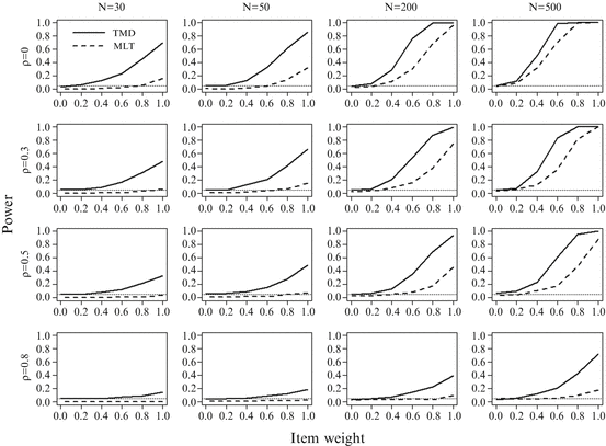
Results for the test length k = 5 + 5 = 10; solid lines represent the T md and the dashed lines represent the MLT. The x-axis gives the weights of the second dimension and the y-axis gives the probability of detecting a model violation (empirical power). The dotted line indicates the nominal significance level of 5 %


In addition, we compared the performance of the quasi-exact test with that of the Martin-Löf test (MLT; as described in Fischer & Molenaar 1995). The MLT is a popular likelihood ratio test of the unidimensionality assumption (see, e.g., Verhelst 2001). As in T md , the data set is split into two subgroups of items (or, as in the current case, two time points). Then the item parameters for the overall sample and for both subsamples are estimated and compared. The MLT can be written as
where w = 1, …, k 1 is the raw score for the first subset of items, u = 1, …, k 2 is the raw score for the second subset of items, r = 1, …, k is the raw score for the overall data matrix (i.e., r = w + u), n r , n w , and n u are the frequencies of the raw scores r, w, and u, n is the number of observations, L (0) c is the conditional likelihood for the item parameters estimated for the overall data matrix, and L (1) c and L (2) c are the conditional likelihoods for the item parameters estimated for the two subsets. The MLT statistic is asymptotically distributed as χ 2 with \( {k}_1+{k}_2-1 \) degrees of freedom.
Results are given in Figs. 2, 3, and 4. The solid lines represent the results for T md and the dashed lines represent the results for MLT. On the x-axis, the weights of the second dimension are displayed, e.g., a value of 0.8 means that the second dimension has a weight of 0.8 and the first dimension of 0.2.

Results for the test length k = 10 + 10 = 20; solid lines represent the T md and the dashed lines represent the MLT. The x-axis gives the weights of the second dimension and the y-axis gives the probability of detecting a model violation (empirical power). The dotted line indicates the nominal significance level of 5 %

Results for the test length k = 20 + 20 = 40; solid lines represent the T md and the dashed lines represent the MLT. The x-axis gives the weights of the second dimension and the y-axis gives the probability of detecting a model violation (empirical power). The dotted line indicates the nominal significance level of 5 %
Overall, the T md was able to protect the nominal significance level of 5 % in all scenarios. The MLT showed deflated type-I error rates. In the shortest test-length scenario (k = 5 + 5 = 10), the type-I error rates for the MLT increase with sample size and were around 5 % at n = 200. This result is in line with results given in Futschek (2014), Verguts and DeBoeck (2001), and Verhelst (2001).
The cases of D 2 > 0 depict the empirical power of the test. In general, the power of both test statistics increased with sample size and decreased with the magnitude of correlation between the latent traits. In addition, however, there were several differences in performance. First, the power of T md increased with test length, whereas the power of the MLT decreased with test length. This can be explained as follows. For constant sample size, longer tests provide more information for generating permutation matrices in the T md approach, but increase the magnitude of estimation errors in the MLT. Second, the T md detected within multidimensionality (range 0.2–0.8) and between multidimensionality (1.0) even in small samples. In addition, the T md detected multidimensionality in large samples and longer tests even if the latent traits were highly correlated. In sum, T md outperformed the MLT regardless of sample size.
Unidimensionality of Change: The Statistic T 4
To test item-specific change or measurement invariance, the statistic T 4 (Ponocny 2001; see also, Koller & Hatzinger 2013) can be used. This statistic can be used to evaluate whether one or more items are easier or more difficult in a predefined group of individuals (or, when measuring change, at t i ) than in another group (or at t j ). The test statistic can be written as
where the x vi of an item in the predefined group of individuals (g = 1, …, G) are summed up over all points in time. When an item within the predefined group of individuals is more difficult than expected under the Rasch model (i.e., the number of correct responses is smaller than expected), the model test is given in Eq. (2). To test the assumption that an item is easier than expected, the model test is
According to Cho et al. (2013), four different violations of measurement invariance across time are of interest: (1) The item parameters differ across person groups (see above). (2) The item parameters differ across time points. (3) The item parameters differ across person groups within a time point. (4) The item parameters differ across time points within a person group. These four potential violations can be analyzed using T 4 by rearranging the data matrix, for example, using the same individuals at t 2 as “virtual” individuals at t 1 and using the time point as splitting variable. Further tests are discussed in Koller and Hatzinger (2013), Koller et al. (2012), and Ponocny (2001).
An empirical power analysis for T 4 (Koller, Maier, & Hatzinger 2015) showed that the type-I error rates of T 4 were far below the nominal level of 5 %. Thus, the test tends to be rather conservative, which may lead to increased type-II error rates. Severe model violations can still be detected with samples of sizes n = 50 or n = 100, and n = 200 seems sufficient to detect weaker violations regardless of the shape of the ability distribution.
Response Independence Between Time Points: The Statistic T 2
The statistic T 2 (Ponocny 2001; see also, Koller & Hatzinger 2013) is well suited to test the assumption of response independence between items. T 2 tests for increased dispersion of raw scores for a set of items. The test statistic can be written as
Var(r (I) v ) is the variance of a subscale I with a minimum of at least two items, which can also mean the same item at t 1 and t 2. According to the variance addition theorem, the variance of a scale that consists of two subscales t 1 and t 2 is defined as \( Var\left({r}_v^{(t1)}\right) + Var\left({r}_v^{(t2)}\right) + 2 \times Cov\left({r}_v^{\left(t1,t2\right)}\right) \) and is expected to increase with the covariance of t 1 and t 2. The model test, given in Eq. (5), tests whether the items are more highly correlated than assumed under the Rasch model.
As for the previously described statistics, the following section describes the results of a simulation study on the type-I error rates and empirical power performance.
Empirical Power Analysis
Violations of the assumption of response independence of two items were simulated as by Marais and Andrich (2008; cf. Andrich & Kreiner 2010). Simulations with 1000 samples each were performed for each combination of sample sizes n = 30, 50, 200, and 500 and test lengths k = 5, 10, 20, and 40. Item and person parameters were drawn from a standard normal distribution with a range of [−2, 2]. For each sample, two moderately difficult items showed violations of the response independence assumption, namely for k = 5: (i = 2, i = 3), k = 10: (i = 5, i = 6), k = 20: (i = 10, i = 11), and k = 40: (i = 20, i = 21). Four different weights were used to simulate different magnitudes of violations (d = 0, 1, 2, and 3). A weight of zero represents the case of no violation, i.e., the type-I error scenarios. Cases of d > 0 correspond to average manifest correlations between items of \( {\overline{r}}_1=.474 \), \( {\overline{r}}_2=.710,\kern0.5em {\overline{r}}_3=.855. \)
Simulation results are displayed in Table 1. In general, the empirical error rates of T 2 (column RM) increased with sample size. The rejection rates were generally far below the nominal level of 5 %. In other words, T 2 tends to be rather conservative, which results in increased type-II error rates. However, small departures from the response independence assumption can be detected even in very small samples. In addition, power increases with sample size and magnitude of violations.
In sum, the power analyses suggest that quasi-exact tests are well suited for small samples. Next, an illustration is given of these tests for the assessment of the three preconditions concerning measurement of change using data from a spatial ability training study.
An Empirical Example: A Spatial Ability Training Study
The data set was collected in the project “Educating Spatial Ability with Augmented Reality” (Kaufmann, Steinbügl, Dünser, & Glück 2005). The study compared the effects of a spatial ability training intervention in an augmented reality (AR)-based three-dimensional setting to a two-dimensional intervention and a no-training control condition. Training effects were measured by a battery of paper-pencil spatial ability tests including the Mental Cutting Test (MCT, CEEB College Entrance Examination Board 1939). Each item of the MCT consists of a perspective drawing of a solid figure that is cut by a plane. Participants are asked to imagine the shape of the cross section and select the correct solution out of five alternatives. The original test consists of 25 items, but, in the current study, a 15-items short version was used.
The sample consisted of 317 high school students, 213 of whom completed both pretest and posttest (51.6 % males; age: M = 17.0, SD = 1.1, min = 14.4, max = 20.5). As no differences between the three-dimensional and the two-dimensional training were found, we focus on comparing the control group (CG; n = 123) to the training group (TG; n = 90) that participated in six weekly training sessions. TG participants were trained either with a computer-aided design software presented two dimensionally on the computer screen or three dimensionally using Augmented Reality (e.g., Kaufmann 2004 2006; Kaufmann & Schmalstieg, 2003). In the following analyses, we use the data from this study to illustrate the usefulness of quasi-exact tests to test preconditions for measuring change.
General results of the training study are reported by Dünser (2005) and Kaufmann et al. (2005); specific results for the MCT can be found in Koller (2010), where quasi-exact tests were used to investigate whether the Rasch model fits the items of the MCT. The Rasch model held at the first and second time point for eight of the 15 items. These items were used here to test the three preconditions for measuring change.
Additionally, it is not possible to apply quasi-exact tests to data including missing values. However, a systematic analysis of the performance of missing value imputation algorithms in the context of quasi-exact tests is clearly beyond the scope of the present chapter. Thus, only the data from 183 individuals who had no missing values across the eight items were used for the analyses. The sample consisted of 81 females and 102 males; 79 of the participants were in the training group.
Results
First, the assumption of unidimensionality across time points was assessed using T md . Analyses were performed separately for the two groups CG and TG. Results suggest that the assumption of unidimensionality holds across time for both groups (p CG = .789; p TG = .998). For example, p CG = .789 means that 78.9 % of the simulated matrices showed the same or a more extreme violation of the unidimensionality assumption. In addition, we analyzed whether the data were sufficiently unidimensional across time for females and males. Again, these results were not significant (p male = .972; p female = .977). Thus, the test measures the same latent dimension across time points.
Even a high correlation between raw scores over time still allows for changes in the difficulty of individual items; for example, one item might have become easier while another became more difficult from t 1 to t 2. Thus, second, the assumption of measurement invariance over time was assessed by splitting the data set according to time point in general and per group and analyzing whether the items at t 2 were significantly easier than expected under the Rasch model (one test for each item). In this analysis, a low p-value for an item suggests that the item was indeed easier at t 2 than at t 1. On the other hand, a very high p-value, for example .90, would imply that 90 % of the simulated matrices showed the same or a lower number of correct answers on the item (i.e., a higher item difficulty) than in the observed matrix. In such cases, we additionally used the statistic T4 to assess whether the item was more difficult at t 2 than assumed under the Rasch model.
The results, given in Table 2, suggest that the first item was easier than expected under the Rasch model in the whole sample and three of the four subgroup analyses. Thus, this item was significantly easier at t 2 than at t 1 for females, for males, and for the training group. For the control group the result was nonsignificant, which suggests that the effect was largely due to the training. On the other hand, item 7 was more difficult at t 2 than at t 1 in the total sample, though not clearly in any of the subgroups. This suggests that training and practice effects did not affected the difficulty of this item. This may imply that this item measures other performance components than the others. These violations of measurement invariance should be considered in the analysis of change and modeling of change effects (e.g., specific change parameters for item groups).
Third, the assumption of response independence over time was investigated for each item separately. The same splitting variables were used as before (i.e., CG vs. TG, females vs. males). As explained earlier, the test statistic T 2, given in Eq. (5), tests whether item responses at t 1 and t 2 are more highly correlated than assumed under the Rasch model. The results in Table 3 suggest several significant response dependencies, most consistently, for items 1, 2, 7, and 8. This type of dependency is typical when the same items were presented at consecutive points in time, and the time interval between two assessments is short. Together with the significant results of the previous analysis, the present results suggest that most participants who solved Item 1 or Item 7 at t 1 also solved these items at t 2, but of those few participants whose response did change, the majority moved from not solving to solving for Item 1 and from solving to not solving for Item 7. Interestingly, the items in the middle of the test (items 3, 4, 5, and 6) showed no significant response dependencies. It may be very interesting to assess the change parameters for both groups of items separately and to compare the results.
In sum, the analyses showed that, on the level of correlations between the raw scores, the assumption of unidimensionality holds for the data set. However, when individual items were inspected, the analyses showed violations of the assumptions of measurement invariance and response independence for some items. These results suggest concrete alternatives for the modeling of change in mental rotation test performance. Although the requirements of classical Rasch-family models for measuring change are not fulfilled, other models can be used to model the changes in this data set. For example, researchers may model several change parameters for the items showing violations of measurement invariance and only one change parameter for the middle group of items. Several item response models are available for measuring change in this way, for example, explanatory item response models (e.g., Cho et al. 2013; Stevenson, Hickendorff, Resing, Heiser, & DeBoeck 2013) or multidimensional Rasch models (e.g., Koller, Carstensen, Wiedermann, & vonEye 2014; Wang, Wilson, & Adams 1998).
Conclusion
In this chapter, we hope to have shown that (1) quasi-exact tests are very well suited to evaluate Rasch model conformity even in small samples, that (2) they can also be used to test important preconditions of item response theory models for measuring change, and (3) yield additional information for model selection.
The empirical power results presented here suggest good performances of all proposed tests. For example, T md is an excellent statistic for the investigation of between-time point and within-time point multidimensionality in small as well as larger samples. Another advantage of T md is the possibility to detect group-specific multidimensionality, even when latent traits are highly correlated. In the simulation, T md outperformed the MLT in all cases.
Of course, further studies are needed to systematically evaluate the behavior of these test statistics under various conditions (see also Koller et al., 2014). For example, future studies should evaluate the behavior of the tests in cases of varying item discrimination and/or multiple model violations. In addition, item position effects which violate one of the underlying mathematical properties of the Rasch model should be investigated in more detail. Furthermore, for T md , further simulation scenarios are needed in which not all items show violations of the unidimensionality assumption, and in which more than two dimensions influence the probability of solving an item.
The current permutation algorithm does not allow missing values. Thus, researchers have to decide a priori whether cases with missing values are removed from the data set or whether missing value imputation methods are carried out prior to the psychometric analysis. First promising results of applying quasi-exact tests to dichotomous data including missing values and trichotomous items are given in Verhelst and Gruber (2013).
References
Adams, R. J., Wilson, M., & Wang, W.-C. (1997). The multidimensional random coefficient multinomial logit model. Applied Psychological Measurement, 21(1), 1–23.
Andersen, E. B. (1973). A goodness of fit test for the Rasch model. Psychometrika, 38(1), 123–140.
Andrich, D., & Kreiner, S. (2010). Quantifying response dependence between two dichotomous items using the Rasch model. Applied Psychological Measurement, 34(3), 181–192.
CEEB College Entrance Examination Board. (1939). Special aptitude test in spatial relations. New York, NY: CEEB.
Cho, S.-J., Athay, M., & Preacher, K. J. (2013). Measuring change for a multidimensional test using a generalized explanatory longitudinal item response model. British Journal of Mathematical and Statistical Psychology, 66(2), 353–381.
Dünser, A. (2005). Trainierbarkeit der Raumvorstellung mit Augmented Reality [Trainability of spatial ability with Augmented Reality]. Unpublished doctoral thesis, University of Vienna, Austria.
Embretson, S. E. (1991). A multidimensional latent trait model for measuring learning and change. Psychometrika, 56(3), 495–515.
Fischer, G. H. (1974). Einführung in die Theorie psychologischer Tests: Grundlagen und Anwendungen. Bern: Huber.
Fischer, G. H. (1976). In D. N. M. de Gruijter & L. J. T. van der Kamp (Eds.), Advances in psychological and educational measurement (pp. 97–110). New York, NY: John Wiley.
Fischer, G. H. (1981). On the existence and uniqueness of maximum-likelihood estimates in the Rasch model. Psychometrika, 46(1), 59–77.
Fischer, G. H. (1989). An IRT-based model for dichotomous longitudinal data. Psychometrika, 54(4), 599–624.
Fischer, G. H. (1995a). Derivations of the Rasch model. In G. H. Fischer & I. W. Molenaar (Eds.), Rasch models: Foundations, recent developments, and applications (pp. 15–38). New York, NY: Springer.
Fischer, G. H. (1995b). Some neglected problems in IRT. Psychometrika, 60(4), 459–487.
Fischer, G. H., & Molenaar, I. W. (1995). Rasch models: Foundations, recent developments, and applications. New York, NY: Springer.
Fischer, G. H., & Ponocny-Seliger, E. (1998). Structural Rasch modeling. Handbook of the usage of LPCM-WIN 1.0. Groningen: ProGAMMA.
Formann, A. K. (1981). Über die Verwendung von Items als Teilungskriterium für Modellkontrollen im Modell von Rasch [The application of items as split criterion for goodness of fit tests for the Rasch model]. Zeitschrift für Experimentelle und Angewandte Psychologie, 28(4), 541–560.
Formann, A. K., & Spiel, C. (1989). Measuring change by means of a hybrid variant of the linear logistic model with relaxed assumptions. Applied Psychological Measurement, 13(1), 91–103.
Futschek, K. (2014). Actual type-I- and type-II-risk of four different model tests of the Rasch model. Psychological Test and Assessment Modeling, 56(2), 168–177.
Gittler, G., & Fischer, G. (2011). IRT-based measurement of short-term changes of ability, with an application to assessing the “Mozart Effect”. Journal of Educational and Behavioral Statistics, 36(1), 33–75.
Glück, J., & Spiel, C. (1997). Item response models for repeated measures designs: Application and limitations of four different approaches. Methods of Psychological Research Online, 2(1). Retrieved from http://www.dgps.de/fachgruppen/methoden/mpr-online/.
Glück, J., & Spiel, C. (2007). Using item response models to analyze change: Advantages and limitations. In A. D. Ong & M. H. M. van Dulmen (Eds.), Oxford handbook of methods in positive psychology (pp. 349–361). Oxford: Oxford University Press.
Holland, P. W., & Wainer, H. (1993). Differential item functioning. Hillsdale, MI: Erlbaum.
Kaufmann, H., & Schmalstieg, D. (2003). Mathematics and geometry education with collaborative augmented reality. Computer & Graphics, 27(3), 339–345.
Kaufmann, H. (2004). Geometry education with augmented reality. Unpublished doctoral thesis, Technical University of Vienna, Austria. Retrieved from http://www.ims.tuwien.ac.at
Kaufmann, H. (2006, August). The potential of augmented reality in dynamic geometry education. Paper presented at the 12th International Conference on Geometry and Graphics (ICGG), Salvador, Brazil.
Kaufmann, H., Steinbügl, K., Dünser, A., & Glück, J. (2005). General training of spatial abilities by geometry education in augmented reality. Annual Review of Cyber Therapy and Telemedicine: A Decade of VR, 3, 65–76.
Koller, I. (2010). Item response models in practice: Testing the assumptions in small samples and comparing different models for repeated measurements. Unpublished doctoral thesis, University of Klagenfurt, Austria.
Koller, I., Alexandrowicz, R., & Hatzinger, R. (2012). Das Rasch Modell in der Praxis: Eine Einführung mit eRm [The Rasch model in practical applications: An introduction using eRm]. Wien: facultaswuv, UTB.
Koller, I., & Hatzinger, R. (2013). Nonparametric tests for the Rasch model: Explanation, development, and application of quasi-exact tests for small samples. Interstat, 1–16. Retrieved from http://interstat.statjournals.net/INDEX/Nov13.html
Koller, I., Maier, M. J., & Hatzinger, R. (2015). An Empirical power analysis of quasi-exact tests for the rasch model: Measurement invariance in small Samples. Methodology, 11(2), 45–55.
Mair, P., Hatzinger, R., & Maier, M. J. (2014). eRm: Extended Rasch Modeling. [Computer software]. R package version 0.15-3. Retrieved from http://CRAN.R-project.org/package=eRm
Marais, I., & Andrich, D. (2008). Formalizing dimension and response violations of local independence in the unidimensional Rasch model. Journal of Applied Measurement, 9(3), 200–215.
Meiser, T. (1996). Loglinear Rasch models for the analysis of stability and change. Psychometrika, 61(4), 629–645.
Ponocny, I. (1996). Kombinatorische Modelltests für das Rasch-Modell. [Combinatorial goodness-of-fit tests for the Rasch model.] Unpublished doctoral thesis, University of Vienna, Austria.
Ponocny, I. (2001). Nonparametric goodness-of-fit tests for the Rasch model. Psychometrika, 66(3), 437–460.
Ponocny, I. (2002). On the applicability of some IRT models for repeated measurement designs: Conditions, consequences, and goodness-of-fit tests. Methods of Psychological Research Online, 7(1), 22–40.
R Core Team. (2014). R: A language and environment for statistical computing. [Computer software] R Foundation for Statistical Computing, Vienna, Austria. Retrieved from http://www.R-project.org/
Rasch, G. (1960). Probabilistic models for some intelligence and attainment tests. Kopenhagen: Danish Institute for Educational Research.
Rost, J. (1990). An integration of two approaches to item analysis. Applied Psychological Measurement, 14(3), 271–282.
Stevenson, C. E., Hickendorff, M., Resing, W. C. M., Heiser, W. J., & DeBoeck, P. A. L. (2013). Explanatory item response modeling of children’s change on a dynamic test of analogical reasoning. Intelligence, 41(3), 157–168.
Verguts, T., & DeBoeck, P. (2001). Some Mantel-Haenszel tests of Rasch model assumptions. British Journal of Mathematical and Statistical Psychology, 54(1), 21–37.
Verhelst, N. D. (2001). Testing the unidimensionality assumption of the Rasch model. Methods of Psychological Research Online, 6(3), 231–271.
Verhelst, N. D. (2008). An efficient MCMC algorithm to sample binary matrices with fixed marginals. Psychometrika, 74(4), 705–728.
Verhelst, N. D., & Gruber, K. (2013). The PCM2-sampler. Paper presented at the Psychoco 2013 (International Workshop on Psychometric Computing), Zurich, Switzerland. Retrieved from http://eeecon.uibk.ac.at/psychoco/2013/
Verhelst, N. D., Hatzinger, R., & Mair, P. (2007). The Rasch sampler. Journal of Statistical Software, 20(4). Retrieved from http://www.jstatsoft.org.
Wang, W.-C., Wilson, M., & Adams, R. J. (1998). Measuring individual differences in change with multidimensional Rasch model. Journal of Outcome Measurement, 2(3), 240–265.
Acknowledgement
This research was partly funded by the Austrian Research Fund, grant nr. P 16803-N12.
Author information
Authors and Affiliations
Corresponding author
Editor information
Editors and Affiliations
Rights and permissions
Copyright information
© 2015 Springer International Publishing Switzerland
About this paper
Cite this paper
Koller, I., Wiedermann, W., Glück, J. (2015). Item Response Models for Dependent Data: Quasi-exact Tests for the Investigation of Some Preconditions for Measuring Change. In: Stemmler, M., von Eye, A., Wiedermann, W. (eds) Dependent Data in Social Sciences Research. Springer Proceedings in Mathematics & Statistics, vol 145. Springer, Cham. https://doi.org/10.1007/978-3-319-20585-4_11
Download citation
DOI: https://doi.org/10.1007/978-3-319-20585-4_11
Publisher Name: Springer, Cham
Print ISBN: 978-3-319-20584-7
Online ISBN: 978-3-319-20585-4
eBook Packages: Mathematics and StatisticsMathematics and Statistics (R0)