Laboratory Models of Free-Surface Flows

Abstract

Hydraulic modeling is the classical approach to investigate and describe complex fluid motion. Many empirical formulas in the literature used for the hydraulic design of river training measures and structures have been developed using experimental data from the laboratory. Although computer capacities have increased to a high level which allows to run complex numerical simulations on standard workstation nowadays, non-standard design of structures may still raise the need to perform physical model investigations. These investigations deliver insight into details of flow patterns and the effect of varying boundary conditions. Data from hydraulic model tests may be used for calibration of numerical models as well. As the field of hydraulic modeling is very complex, this chapter intends to give a short overview on capacities and limits of hydraulic modeling in regard to river flows and hydraulic structures only. The reader shall get a first idea of modeling principles and basic considerations. More detailed information can be found in the references.

1 Introduction

For more than 500 years, people have tried to better understand the nature of complex flows. For instance, several famous records and sketches on flow phenomena were published by Leonardo Da Vinci in the late 15th century. Sir Isaac Newton (1642–1727) was the first to develop basic approaches on the similitude between a prototype and its scaled reproduction, i.e. the model. These approaches were advanced by other researchers developing modeling laws which are well recognized nowadays. These model laws were first applied to scaled models at the end of the 19th century. In particular, William Froude (1810–1879) and Osborn Reynolds (1842–1912) shall be mentioned in the context as representatives of many important individuals of fluid mechanics in these days.

Hughes (1993) stated that physical modeling is still an important technique to solve hydraulic engineering problems even in a time that computers become more and more powerful and numerical models more reliable. Even two decades later, this statement is still valid.

Hydraulic modeling allows to directly face the effects on flow features induced by changes of boundary conditions. Physical hydraulic models may also be operated to verify theoretical and numerical models or to draw some conclusion in regard to flow phenomena that are still not fully understood to date. Further development of measurement techniques allows for new investigation methods and gives high-precision results. Some up-to-date equipment are illustrated in Fig. 9.1.

Fig. 9.1

Measuring devices for laboratory studies. a Ultrasonic displacement sensor for accurate measurement of water levels. b Acoustic Doppler Velocimeter (ADV) for measuring of local three-dimensional velocity components (here installed in the non-aerated part of stepped weir before submerging into water)

On the other hand, the setup of a physical model is often relatively expensive and time-intensive. A change of boundary conditions is oftentimes not trivial and needs to be considered in the early stages of planning. Later adaption to other conditions may be difficult.

2 Similitude

In order to extend the findings from a scaled physical model to prototype scale, hydromechanical similitude between both scales must be guaranteed. This means that a geometric, kinematic and dynamic similitude are needed to ensure a similar motion and, by consequence, similar forces acting in the fluid. In a flowing water body, the following forces must be considered (forces due to elasticity are neglected for water as an incompressible fluid):

• a force due to acceleration of the fluid (inertia) $F_{i}$,

• a force due to gravity $F_{g}$,

• a force due to pressure in the flow field $F_{p}$,

• a force due to inner friction (viscosity) $F_{v }$,

• a force due to surface tension at the air-water interface $F_{s}$.

It yields the following balance of forces:

$$F_{i} = F_{g} + F_{p} + F_{v} + F_{s}$$

(9.1)

Considering a general length $L$ and time $T$ and neglecting $F_{p}$ because it is a dependent force, Eq. 9.1 becomes:

$$\rho \times L^{3} \times L/T^{2} = \rho \times L^{3} \times g + \mu \times \frac{L/T}{L} \times L^{2} + \sigma \times L$$

(9.2)

where $\rho$ is the density of water in [t/m³], $g$ is the gravity acceleration in [m/s²], $\mu$ is the dynamic viscosity in [kg/(m × s)] and $\sigma$ is the surface tension in [kN/m]. A dynamic similitude now claims that all forces have the same scale factor:

$$\frac{{F_{i,N} }}{{F_{i,M} }} = \frac{{F_{g,N} }}{{F_{g,M} }} = \frac{{F_{v,N} }}{{F_{v,M} }} = \frac{{F_{s,N} }}{{F_{s,M} }}$$

(9.3)

and by consequence

$$\frac{{\rho_{N} \times L_{N}^{4} /T_{N}^{2} }}{{\rho_{M} \times L_{M}^{4} /T_{M}^{2} }} = \frac{{\rho_{N} \times L_{N}^{3} \times g_{N} }}{{\rho_{M} \times L_{M}^{3} \times g_{M} }} = \frac{{\mu_{N} \times L_{N}^{2} /T_{N} }}{{\mu_{M} \times L_{M}^{2} /T_{M} }} = \frac{{\sigma_{N} \times L_{N} }}{{\sigma_{M} \times L_{M} }}$$

(9.4)

with index $N$ referring to prototype scale and index $M$ to model scale, respectively. Full hydromechanical similitude could be achieved if the model would be operated by a fluid with density, viscosity and surface tension that fulfills this constraint. Unfortunately, this fluid does not exist and models are commonly operated by the same fluid as in nature, i.e. water. With the length scale $\lambda_{L} = L_{N} /L_{M}$, the time scale $\lambda_{T} = T_{N} /T_{M}$ as well as ${{\rho_{N} } \mathord{\left/ {\vphantom {{\rho_{N} } {\rho_{M} }}} \right. \kern-0pt} {\rho_{M} }} = 1,\,{{\mu_{N} } \mathord{\left/ {\vphantom {{\mu_{N} } {\mu_{M} }}} \right. \kern-0pt} {\mu_{M} }} = 1,\,{{\sigma_{N} } \mathord{\left/ {\vphantom {{\sigma_{N} } {\sigma_{M} }}} \right. \kern-0pt} {\sigma_{M} }} = 1\,{\text{and}}\,{{g_{N} } \mathord{\left/ {\vphantom {{g_{N} } {g_{M} }}} \right. \kern-0pt} {g_{M} }} = 1$, Eq. 9.4 becomes:

$$\frac{{\lambda_{L}^{4} }}{{\lambda_{T}^{2} }} = \lambda_{L}^{3} = \frac{{\lambda_{L}^{2} }}{{\lambda_{T} }} = \lambda_{L}$$

(9.5)

It must be noted that this equation is only valid for $\lambda_{L} = \lambda_{T} = 1$, i.e. the prototype scale. It is not possible to properly scale all acting prototype forces in a scaled hydraulic model. Every scaled model implements certain errors. However, this error can be minimized if the most relevant counter-acting force is considered together with the inertia force and properly scaled. For free-surface flows which is dealt with in this chapter, the predominant force is gravity.

3 Froude’s Law

The relation between the inertia force and the gravity force in open channels is generally expressed by the Froude number:

$${\text{F}} = \sqrt {\frac{\text{inertia}}{\text{gravity}}} = \sqrt {\frac{{\rho \times V \times v^{2} /L}}{\rho \times V \times g}} = \frac{v}{{\sqrt {g \times L} }}$$

(9.6)

where $V$ is the volume of the water body moving with the velocity $v$.¹

The basic idea of Froude’s law is that the dimensionless Froude number is the same in model and nature for a similar flow condition. This means that a sub-/supercritical flow in nature must be sub-/supercritical in the model as well. The flow may then be described by the same governing differential equations with transferrable boundary conditions upstream or downstream. Identical Froude numbers yield:

$$\frac{{v_{N} }}{{\sqrt {g \times L_{N} } }} = \frac{{v_{M} }}{{\sqrt {g \times L_{M} } }}$$

(9.7)

On this basis, the scaling factors for all physical properties may be derived, e.g.:

• Velocity factor: $\lambda_{v} = {{v_{N} } \mathord{\left/ {\vphantom {{v_{N} } {v_{M} }}} \right. \kern-0pt} {v_{M} }} = \sqrt {{{L_{N} } \mathord{\left/ {\vphantom {{L_{N} } {L_{M} }}} \right. \kern-0pt} {L_{M} }}} = \sqrt {\lambda_{L} }$

• Time factor: $\lambda_{T} = {{\lambda_{L} } \mathord{\left/ {\vphantom {{\lambda_{L} } {\lambda_{v} }}} \right. \kern-0pt} {\lambda_{v} }} = {{\lambda_{L} } \mathord{\left/ {\vphantom {{\lambda_{L} } {\sqrt {\lambda_{L} } }}} \right. \kern-0pt} {\sqrt {\lambda_{L} } }} = \sqrt {\lambda_{L} }$

• Discharge: $\lambda_{Q} = \lambda_{v} \times \lambda_{A} = \sqrt {\lambda_{L} } \times \lambda_{L}^{2} = \sqrt {\lambda_{L}^{5} }$

• etc.

3.1 Model Accuracy

Data from the laboratory needs to be scaled to prototype dimensions according to the appropriate model scale factors. However, the modeler must be aware of inaccuracies which may derive from different sources. In detail, model effects and scale effects may occur.

3.1.1 Model Effects

Model effects may arise from an inappropriate idealization of the prototype conditions in the laboratory. For example, three-dimensional flow patterns in the stilling basin downstream of a weir model (see Fig. 9.2) may not fully develop when the model is installed in a narrow flume. Depending on the purpose of such a study, this effect may be more (e.g. stilling basin design) or less (e.g. determination of weir coefficient) severe. Reflections from walls may also lead to some undesired effect as well as incorrect water levels due to wall effects when water levels are visually investigated through a transparent sidewall. On the other hand, some effects being present in the prototype system are difficult to reproduce, e.g. raised water levels by wind. These exemplary problems emphasize that some experience is required by the modeler in order to avoid or at least to recognize such effects and in this case, to evaluate those in regard to not misinterpret the data.

Fig. 9.2

Model investigation on stilling basin performance downstream of a steep stepped spillway (Bung et al. 2012), channel width is 1 m to avoid model effects

3.1.2 Scale Effects

As discussed above, model laws, such as the Froude’s law for open channel flows, are based on the idea to just account for the major force counter-acting the inertia force. This assumption is reasonable as long as the model scale does not fall below a critical value where other forces may become significant. A few simple examples shall illustrate this problem:

• If the Froude’s law is considered, the scale factor for the dimensionless Reynolds number² in a model with identical fluid becomes $\lambda_{R} = \lambda_{v} \times \lambda_{L} = \lambda_{L}^{3/2}$. Thus, the Reynolds number is never properly scaled in a Froude model and viscosity effects may lead to disturbed results. Considering the precondition that the flow resistance $f$ in model and prototype must be equal, it has to be ensured that hydraulic rough conditions are met in the model (i.e. the flow resistance $f$ is no more dependent on R, see Fig. 9.3) which in turn is only met in large scale models. Alternatively, the modeler may come up with the idea to chose a smaller surface roughness $k$ in order to ensure a properly scaled $f$ even for a small Reynolds number in the model. However, it must be recognized that scaling of bed roughness is generally difficult, particularly for a small roughness in prototype, e.g. for a concrete surface.

  Fig. 9.3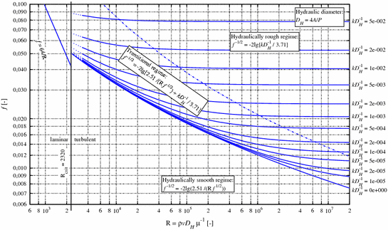

  

  Moody diagram for determination of flow resistance factor $f$ as a function of relative roughness $k/D_{H}$ (with $D_{H} = 4 \times A/P$ the hydraulic diameter, $A$ the cross-sectional area and $P$ the wetted perimeter) and Reynolds number $R$

• A small scale weir overflow model becomes more and more affected by surface tension when the water level at the weir crest is low for a given flow velocity.

• Investigations on sediment transport may be affected by scale effects when particles need to be scaled to a smaller size, thus reaching undesired cohesive characteristics.

• Laboratory studies with focus on air-water flows, e.g. hydraulic jump downstream of a weir, must be modeled in large scale as air bubbles in prototype tend to break up when reaching a critical size, particularly in turbulent flows. By consequence, air bubbles have roughly the same size, in model and in prototype, and are thus not properly scalable. Air bubble lift forces may play a more significant role in model as in nature.

Numerous studies have been performed to determine the critical scale to prevent scale effects. Several publications on scale effects for models with different focus are included in Kobus (1984). Recently, a comprehensive review on critical model scales was presented by Heller (2011). If no information on scale effects and minimum model scales is found in the literature, the modeler should consider evaluating a series of models and differing size scale before setting up the final full model in order to check from which scale on the data lead to differing results when scaled up to prototype scale according to the relevant scale factors. Laminar flows however, where the flow depth is low and the velocity is small, should be modeled in prototype scale to reproduce the viscous effects correctly.

4 Open Channels

4.1 Models with Fixed Bed

Physical models with fixed beds are used with different focuses. In earlier times, the main interest was to determine water levels and flooded ares for different flood events. Other concerns could be be found in the effects of river training measures or the formation of 2D or 3D flow patterns (e.g. eddy formation in groin fields). It must be confessed that such studies are commonly performed numerically nowadays. Large laboratory capacities in terms of space and discharge are required to operate physical river models. Consequently, such studies are very cost-intensive while numerical 2D and 3D river models are available for free as open-source codes. However, physical river models are still a useful method to investigate more complex flow situations, which may be caused by e.g. jet formation and mixing procedures at an cooling water outfall structure (see Sect. 9.5.4).

4.2 Models with Movable Bed

River models with movable beds are used for investigation of bed load and sediment transport. Local erosion and deposition processes may be in the focus for waterways modeling and in models of inlet structures to hydropower plants. Such models need to fulfill the same hydraulic similitude as developed above, but further considerations on particle dynamics are needed. These particle dynamics can be described by the sediment Froude number

$${\text{F}}_{s} = \frac{{\tau_{0} }}{{g \times \left( {\rho_{s} - \rho } \right) \times d_{s} }}$$

(9.8)

and the sediment Reynolds number

$${\text{R}}_{s} = \frac{{\sqrt {\tau_{0} \times \rho } \times d_{s} }}{\mu }$$

(9.9)

where $\tau_{0}$ is the bed shear stress, $\rho_{s}$ the particle density and $d_{s}$ the particle diameter. Both dimensionless numbers are known from the famous Shields diagram for onset of particle movement and must be the same in model and prototype. With this precondition, relevant scale factors for sediment modeling may be derived, such as the particle size scale and the particle time scale, and a model sediment material (and grain size curve) can be chosen. For further information see (ASCE 2000) and (Kobus 1980). One resulting difficulty is caused by the particle time scale which differs from the flow time scale derived above. Sediment movement is faster in the model than in the nature. The modeler may address this issue by comparing the model data with sediment data from the field.

The total bed load or sediment load being transported through the model can be measured by collecting and weighing the material at the model outflow boundary. Depending on the test duration, the model size and the study purpose, it may be necessary to ensure that the same amount of material is added at the inflow boundary in order to provide enough material for the test.

4.3 Distorted Models

Model scales for large river models are often limited due to given space and/or discharge capacity in the laboratory. However, too small model scale may result in an improper scaling of Reynolds numbers and friction factors. One technique to overcome this problem is to set up a distorted model in which the length scale number in vertical direction $\lambda_{L,v}$ is smaller than the length scale number in horizontal direction $\lambda_{L,h}$. By distorting the model, the flow velocity and flow depth is increased compared to an undistorted model with $\lambda_{L,h}$ in all directions and a larger Reynolds number is obtained (the influence of surface tension is decreased as well). By consequence, a hydraulic rough condition can set in. In this case, different scale factors must be regarded for different hydraulic parameters which can be found in Kobus (1980). It must be noted that the scaling of surface roughness in a distorted model is even more difficult than in an undistorted model. Proper scaling of roughness needs to be achieved by calibration using prototype data. It must also be taken into account that three-dimensional flow patterns, such as vertical eddy formation around a bottom structure, become difficult to transfer to the prototype in a distorted model ASCE (2000). The applicability of distorted models must be carefully evaluated. Some model tests, e.g. the three-dimensional mixing procedure in the near field of an outfall structure, do not allow model distortion.

4.4 Vegetational Flow

In the recent past, several studies were conducted which focused on the effects of vegetation in natural channels on the river flow. One major feature which must be addressed is that vegetation may be deformed under hydrodynamic conditions and the absolute roughness becomes a function of discharge. In hydraulic models, the vegetation is often modeled by some artificial plants which must then have a similar geometry and stiffness. Proper scaling of the vegetation characteristics is not trivial. The modeler may also pay attention to river vegetation when a study on sediment transport is planned as some relevant interaction can occur. Vegetational flow features are presented in detail in Aberle (2015) (this issue). The flow resistance nature of the vegetation can also change seasonally. For further information on the topic, the reader is referred to that chapter which also includes some exemplary model studies.

4.5 Debris and Ice

Modeling of debris and ice are challenging (and rare) tasks which may come up in early design stages of weirs, locks or hydropower plants and which require correct reproduction of drift and accumulation of ice and debris. For some questions, special attention must be paid to the proper modeling of the material to be used in the laboratory to reproduce the rigidity and eventually the thermal properties in case of ice. Furthermore, wind may play an important role, particularly when the load on a structure is of interest. Debris and ice modeling are no standard problems, see ASCE (2000) for additional details regarding derivation of relevant scale factors.

5 Hydraulic Structures

5.1 Aerated Flow

5.1.1 Introduction

Aeration mainly occurs in high-turbulent flows. The most important causes for aeration in rivers are hydraulic jumps and mixing downstream of weir overflows (see Fig. 9.4). For hydraulic jumps, the amount of entrained air depends on the inflow Froude number. In case of a weir, a growing turbulent boundary layer develops at the weir crest. If the structure is high enough, self-aeration sets in at the point of intersection of the boundary layer and water surface. In both cases, the entrainment of air leads to a bulking of the flow depth, i.e. the air bubbles are transported along the whole water column which generates higher water levels than for clear water. Knowledge of the amount of entrained air is thus important for the hydraulic design, e.g. for sidewall heights. Consideration of entrained air is also relevant for energy dissipation calculations when the bulked flow depth is measured in the laboratory.

Fig. 9.4

Aeration at hydraulic structures. a Aeration at a weir downstream of Oker dam in Germany; note the strong aeration at the bottom outlet in the background. b Aeration on a cross-bar block ramp due to local hydraulic jumps (Oertel and Bung 2012)

Some weirs are used specifically to force air entrainment in rivers in order to re-oxygenate the water. Oxygen is transferred across the air-water interface of the bubbles. However, it must be considered that air bubbles are roughly of the same size in model and in prototype. Scale effects are thus very likely when oxygenation tests are performed in scaled model.

5.1.2 Air-Water Mixture

Description of the air-water mixture body becomes difficult when the flow is fully aerated. Close to the bottom, the air-water mixture is characterized by air bubbles transported in the water, while in higher elevation larger air pockets being entrapped between surface waves may be found (Wilhelms and Gulliver 2005). Above this elevation, mainly ejected droplets are found (see Fig. 9.5). By consequence, void fraction $C$ is non-uniformly distributed along the water column. A typical void fraction profile for a stepped weir is also presented in Fig. 9.5.

Fig. 9.5

Air-water mixture in self-aerated high-speed flows on a stepped weir model (width 50 cm, step height 6 cm, slope 1:2, discharge 35 l/s). a Photograph captured by a high-speed camera with 700 fps; the markers indicate the water level with 90 % time-averaged void fraction which is often taken into account as idealized water surface. b Void fraction profile measured at the stepped edges with a conductivity probe

In most studies, air-water flow properties were measured by means of intrusive needle probes which consist of fine tips that pierce the air bubbles. These probes work on basis of different conductivity characteristics between air and water (conductivity probe) or different optical refraction characteristics (fibre optical probes). The principle of these probes is discussed in Chanson (2002) amongst others. Recent studies show that modern non-intrusive methods may also be applied. Leandro et al. (2014) present a calibration method which can be used to obtain air concentration profiles and velocity fields from high-speed camera movies. Even the data from ultrasonic displacement sensors, normally known to be inaccurate in flows with irregular surface, can give some reasonable results as demonstrated by Chachereau and Chanson (2011) in hydraulic jumps and Bung (2013) in self-aerated chute flows.

5.1.3 Oxygenation Potential

Due to the large amount of air-water interface in aerated open channel flows, the oxygenation potential is high. This may be of interest to enrich water from a reservoir with oxygen when discharged to the downstream river. As mentioned above, scale effects cannot be avoided when investigations are performed on a scaled model due to similar air bubble sizes in the model and in prototype. However, in large-scale models the measured data give at least an idea of relative potentials when different situations are compared. Several recent studies presented direct oxygenation measurements where the water was de-oxygenated by addition of sodium sulfite before the test and the oxygen content recorded over time [(Avery and Novak 1978), (Bung 2011), (Essery et al. 1978), (Toombes and Chanson 2005) a.o.]. The references include more information on the technique, further information may also be found in ASCE (2007).

5.1.4 Scale Effects

Many publications address the very important topic of scale effects in aerated flows. Accordingly, model tests should be carried out on large-scale models. For self-aerated flows, a minimum scale is often given by 1:10 [e.g. (Chanson 1996)] and a minimum Reynolds number of 10⁵ at the aeration point [e.g. (Kobus 1985)]. Newer publications identify a minimum Reynolds number of 2 to 3 × 10⁵ to properly represent the turbulent properties [e.g. (Pfister and Chanson 2012)].

5.2 Scouring

For the modeling of scour processes, the basic considerations on particle dynamics from Sect. 9.4.2 dealing with sediment transport models are still valid. Scouring models are typically detailed models of flow at hydraulic structures, i.e. with larger scale than river models with movable beds. For the operation of a scour model, two important aspects are essential:

• 1. Scouring is a long-term process in nature which takes relatively less time in the model due to different time scales as discussed in Sect. 9.4.2. For the safe design of hydraulic structures the maximum values for the scour depth and size are important, i.e. the equilibrium state which sets in after a certain time under steady-state flow conditions. It must thus be ensured that this equilibrium state is obtained in the model. As scour dimensions are usually measured in dry conditions (after the model run), a sensitivity analysis in terms of a series of model runs is required for comparison of results from tests with different duration.

• 2. As mentioned above, the scour dimensions are measured in dry conditions. It must be ensured by the operator that the scour is not deformed during the run-off process. Seepage through the loose bed may lead to erosion in the scour hole and adulterate the results.

Usually, laser distance meters are used for measuring of scour depth. The measuring spot is tiny and the application in small scour becomes possible. Acoustic displacement meters are characterized by a larger measuring area due to spreading of the acoustic beam. These probes are less accurate for small scour holes where the acoustic beam size is in the range of the scour dimensions.

More information on scouring processes including some exemplary model studies can be found in Pagliara (2015) (this issue).

5.3 Structural Vibration

Knowledge about potential vibrations is essential in early design stages for any regulation structure. Severe damages may happen in case where excitation frequencies coincide with structural frequencies, i.e. the eigenfrequencies which depend on the structure’s mass and stiffness. Besides a self-excited vibration which may be induced by a gate movement, flow-induced vibration are the most important vibration source. In this case, flow turbulence leads to fluctuating pressures around the structure. In general, two different ways of modeling are possible for vibration tests.

• 1. Proper modeling and scaling of all structural parameters, i.e. dimensions, mass and stiffness: Structural vibrations can then be directly inspected. However, scaling of the structure’s stiffness is very difficult, particularly for complex structures.

• 2. Proper modeling of the hydraulic conditions and the structure’s dimensions only (see Fig. 9.6): The structure’s mass and stiffness are disregarded and a fully rigid model is built. In this case, only the external flow fluctuations can be measured in the model. Th excitation potential is then evaluated by comparison of the major frequencies with mathematically derived eigenfrequencies of the structure. The modeler must then decide which eigenfrequencies are relevant for a global vibration. Generally, eigen modes higher than the 6–7th modes may be considered to lead to local, less severe vibration modes only.

  Fig. 9.6

  

  Rigid physical model (scale 1:35) of a high-head radial gate for vibration test purposes (Schlurmann and Bung 2012), note the pressure transducers installed in bottom and at the skin plate of the gate used to measure pressure fluctuations

The phenomenon of structural vibration in hydraulic engineering is addressed in ICOLD (1996). General information on its modelling is presented by Kobus (1980) while exemplary studies may be found in Chowdhury et al. (1997) and Schlurmann and Bung (2012).

5.4 Outfalls

Effluents from outfall structures often have a different density than the ambient water body. Thus, upward (positive) or downward (negative) directed lift forces due to the different specific weight affect the turbulent diffusion. In this case, a densimetric Froude number³ becomes relevant (Turner 1966):

$${\text{F}}_{d} = \frac{v}{{\sqrt {g \times \left( {{{\varDelta \rho } \mathord{\left/ {\vphantom {{\varDelta \rho } \rho }} \right. \kern-0pt} \rho }} \right) \times L} }}$$

(9.10)

where $\varDelta \rho$ is the difference in density between effluent and ambient water.

Generally, the near field around the outfall must be distinguished from the far field. In the near field, the mixing is mainly caused by small-scale turbulence between the jet and the surrounding water body. In the far field, large-scale turbulent diffusion maintains the mixing process. Thus, near field investigations need a detailed reproduction of hydraulic and geometrical conditions at the structure, while for far field investigations proper modeling of the river characteristics is required. However, the transition between near field and field is hard to define. The modeler should therefore ensure correct modeling for all regions.

As the turbulence is the decisive parameter for the mixing, the modeler must pay attention to possible scale effects. As mentioned earlier, the Reynolds number can never be scaled correctly in a Froude model. According to Kobus (1980), a minimum Reynolds numbers of 2000 for the jet and 3000 for the river, respectively, must be achieved to avoid those scale effects. It must be noted that degradation time scales of pollution due to biological and chemical processes cannot be scaled.

Models are mostly operated by adding some tracers which show a comparable mixing characteristic as the real effluent. For example, the tracer could have a certain salinity leading to a different density. The mixing could then be observed by measuring the decreasing salinity at numerous downstream cross sections. In laboratories with closed water cycles, the modeler must consider the travel time of the tracer to re-arrive at the model to avoid an undesired increase of density at the model inlet.

References

Aberle J (2015) Hydrodynamics of vegetated channels. In: Rowinski PM, Radecki-Pawlik A (eds) Rivers—physical, fluvial and environmental processes, Springer (this issue), Berlin
Avery ST, Novak P (1978) Oxygen transfer at hydraulic structures. J Hydr Div HY11:1521–1540
ASCE (2000) Hydraulic modeling: concepts and practice. Bulletin 7, ASCE manuals and reports on engineering practice. American Society of Cicvil Engineers, Reston
ASCE (2007) Measurement of oxygen transfer in clean water (ASCE standard 2-06). American Society of Cicvil Engineers, Reston
Bung DB (2011) Fließcharakteristik und Sauerstoffeintrag bei selbstbelüfteten Gerinneströmungen auf Kaskaden mit gemäßigter Neigung (Flow characteristics and oxygenation in self-aerated skimming flows on embankment cascades, in German). ÖWAW 3–4(2011):76–81
Bung DB, Sun Q, Meireles I, Viseu T, Matos J (2012) USBR type III stilling basin performance for steep stepped spillways. In: 4th IAHR symposium on hydraulic structures, Porto
Bung DB (2013) Non-intrusive detection of air–water surface roughness in self-aerated chute flows. J Hydr Res 51(3):322–329
Chachereau Y, Chanson H (2011) Free-surface fluctuations and turbulence in hydraulic jumps. Exp Thermal Fluid Sci 35(6):896–909
Chanson H (1996) Air bubble entrainment in free-surface turbulent shear flows. Academic Press, San Diego
Chanson H (2002) Air-water measurements with intrusive phase-detection probes: can we improve their interpretation? J Hydr Eng 128(3):252–255
Chowdhury MR, Hall RL, Pesantes E (1997) Flow-induced vibration experiments for a 1:25-scale-model flat wicket gate. Technical report SL-97-4, U.S. Army Corps of Engineers. Waterways Experiment Station, Louisville
Essery ITS, Tebutt THY, Rasaratnam SK (1978) Design of spillways for re-aeration of polluted waters. Technical report 72. Construction Industry Research and Information Association (CIRIA), Birmingham
Heller V (2011) Scale effects in physical hydraulic engineering models. J Hydr Res 49(3):293–306
Hughes SA (1993) Advanced series on ocean engineering. In: Liu PL-F (ed) Physical models and laboratory techniques in coastal engineering, vol 7. World Scientific Publishing, Singapore
ICOLD (1996) Vibrations of hydraulic equipment for dams: review and recommendations. Bulletin 102, Commission International des Grands Barrages/Committee on hydraulics for dams, Paris
Kobus H (1980) Hydraulic modelling. Bulletin 7. German Association for Water Resources and Land Improvement. Parey, Hamburg
Kobus H (1984) Symposium on scale effects in modelling hydraulic structures. University of Stuttgart, Stuttgart, Hydraulic Engineering Institute
Kobus H (1985) An introduction to air-water flows in hydraulics. University of Stuttgart, Hydraulic Engineering Institute, Stuttgart
Schlurmann T, Bung DB (2012) Experimental investigation of flow-induced radial gate vibrations at Lower Subansiri dam. In: 6th Chinese–German joint symposium on hydraulic and ocean engineering, Keelung
Leandro J, Bung DB, Carvalho R (2014) Measuring void fraction and velocity fields of a stepped spillway for skimming flow using non-intrusive methods. Exp Fluids. doi:10.1007/s00348-014-1732-6
Oertel M, Bung DB (2012) Characeristics of cross-bar block ramp flows. In: 4th IAHR symposium on hydraulic structures, Porto
Pagliara S (2015) Energy dissipation and scouring problems in rivers. In: Rowinski PM, Radecki-Pawlik A (eds) Rivers—physical, fluvial and environmental processes, Springer (this issue), Berlin
Pfister M, Chanson H (2012) Discussion of scale effects in physical hydraulic engineering models. J Hydr Res 50(2):244–246
Riester JB, Bajura RA, Schwarz SH (1980) Effects of water temperature and salt concentration on the characteristics of horizontal buoyant submerged jets. J Heat Transfer 102:557–562
Toombes L, Chanson H (2005) Air–water mass transfer on a stepped waterway. J Environ Eng 131(10):1377–1386
Turner JS (1966) Jets and plumes with negative or reversing buoyancy. J Fluid Mech 26:779–792
Wilhelms SC, Gulliver JS (2005) Bubbles and waves description of self-aerated spillway flow. J Hydr Res 43(5):522–531
Author information
Authors and Affiliations
Corresponding author
Editor information
Editors and Affiliations
Rights and permissions
Copyright information
© 2015 Springer International Publishing Switzerland
About this chapter
Cite this chapter
Bung, D.B. (2015). Laboratory Models of Free-Surface Flows. In: Rowiński, P., Radecki-Pawlik, A. (eds) Rivers – Physical, Fluvial and Environmental Processes. GeoPlanet: Earth and Planetary Sciences. Springer, Cham. https://doi.org/10.1007/978-3-319-17719-9_9
Download citation
DOI: https://doi.org/10.1007/978-3-319-17719-9_9
Published:
Publisher Name: Springer, Cham
Print ISBN: 978-3-319-17718-2
Online ISBN: 978-3-319-17719-9
eBook Packages: Earth and Environmental ScienceEarth and Environmental Science (R0)