Dynamic Process Analysis

Abstract

Dynamic analysis has been increasingly gaining importance over the last few years in the field of process design. Largely because novel process designs are more efficient, if the controllability is considered during the detailed engineering stage. By means of dynamic simulation, it is possible to monitor the behavior of the main process variables when subjected to disturbances typical of an industrial plant operation.

These keywords were added by machine and not by the authors. This process is experimental and the keywords may be updated as the learning algorithm improves.

8.1 Introduction

Dynamic analysis has been increasingly gaining importance over the last few years in the field of process design . Largely because novel process designs are more efficient, if the controllability is considered during the detailed engineering stage. By means of dynamic simulation , it is possible to monitor the behavior of the main process variables when subjected to disturbances typical of an industrial plant operation.

Furthermore, the possibility of suggesting different control strategies and assess their effect on the operability makes possible to study several scenarios in a relatively short time. Generally speaking, new plant designs and control strategies must guarantee product quality, process safety, equipment protection, and compliance to environmental regulations. All these fields can be considered when developing dynamic models of existing processed or new designs.

In this chapter, a series of case studies is presented; in these, some of the above mentioned process parameters are analyzed, willing to provide the reader with the fundamentals for the analysis of future simulations and also aiming to provide a tool to expand the understanding of fundamental process control principles.

8.2 General Aspects

The behavior of a process with time is subject to the nature and the way the system feeds are applied. The study of the dynamic characteristics of a process allows to determine what the best control strategy is considering that many of the systems present in industry are highly nonlinear in nature. The challenge in process control lies in that most of the times there is a dependence of the process response with time; this causes the process variables to experiment a delay on the response time. This dependence with time is known as the process dynamics and it is necessary to be familiar with it before approaching the problem of process control.

The dynamic behavior characteristics of a system, mechanic , chemical, thermic, or electric are defined by any of the following effects: inertia, capacitance, resistance, and dead time.

Consider a system where a tank receives a liquid stream Fin that accumulates until a certain level and an outlet stream at a rate of F _out. When developing a mathematical model that allows describing the behavior of the tank level the following is stated:

The mass balance in the tank can be written as:

$$ \frac{\mathrm{d}V}{\mathrm{d}t}={F}_{\mathrm{in}}-{F}_{\mathrm{out}} $$

(8.1)

Then, it can be written as a function of the height h of liquid in the tank keeping in mind that the cross sectional area is constant.

$$ A\frac{\mathrm{d}h}{\mathrm{d}t}={F}_{\mathrm{in}}-{F}_{\mathrm{out}} $$

(8.2)

Likewise, it can be stated that the outlet flow rate F _out is defined by

$$ {F}_{\mathrm{out}}=\frac{h}{C} $$

(8.3)

where:

• V: liquid volume in the tank

• h: liquid height

• A: cross sectional area of the tank

• F _in: inlet flowrate

• F _out: outlet flowrate

• C: flow coefficient (show the dependence of the outlet flow with the liquid height)

Equation 8.2 can be reordered as:

$$ A\frac{\mathrm{d}h}{\mathrm{d}t}={F}_{\mathrm{in}}-\frac{h}{C} $$

(8.4)

$$ A\frac{\mathrm{d}h}{\mathrm{d}t} + \frac{h}{C}={F}_{\mathrm{in}} $$

(8.5)

$$ A\frac{\mathrm{d}h}{\mathrm{d}t} + \frac{h}{C}={F}_{\mathrm{in}} $$

(8.6)

Equation 8.6 corresponds to the general first-order differential equation, it can be written in terms of a steady state gain K and a time constant τ. Having:

$$ \tau \frac{\mathrm{d}y}{\mathrm{d}t}+y={K}_u(t) $$

(8.7)

where y(t) is the output function and u(t) is the process input that when modified affects the output. As shown in Fig. 8.1

Fig. 8.1

Scheme of a reservoir tank for liquids

In this way, (8.6) can be finally written as

$$ \tau \frac{\mathrm{d}h}{\mathrm{d}t}+h=K{F}_{\mathrm{in}} $$

(8.8)

where τ = AC and K = C.

It can be seen that the time constant τ is determined by the cross sectional area of the tank, in other words, by the geometry of the tank. Also, the gain of the process is given by the characteristics of the outlet valve of the system.

In general the process gain K is defined as the relationship between the change in the process output and a change in the process input. In this example F _in corresponds to the input and the height h to the output. In steady state, the first term of (8.8) equals zero and it can be solved for K.

The time constant represents the response speed of the system. For first-order systems, when a step type disturbance occurs, there is a time interval τ in which the process variable changes 63 % of the total change, see Fig. 8.2.

Fig. 8.2

First-order system response

Process dead time (θ) of a process is defined as the time between a change in an input variable and the detection of a change in the output variable . In some systems, the change in the output variable when a disturbance occurs is almost instantaneous thus the dead time is close to zero. However, with most of the physical and chemical systems dead times can be significant depending on the process nature and the location of the measurement instruments. Frequently dead time is caused by mass and heat transfer gradients in different points of the process.

8.2.1 Process Control

In the processing industry, there is an increasing interest for properly standardized processes as well as for ensuring product quality. Furthermore, environmental regulations and process safety require proper control mechanisms that allow for the fulfillment of these requirements.

Given the ever changing economic conditions and the competitiveness of the market, process control becomes important to provide efficient processes and high quality products. The operability of more integrated processes with fewer degrees of freedom makes room for error smaller. Hence, more efficient control strategies are required (Luyb en2002; Pe rry1992).

Take a fermentation reactor as an example, initially it is required that all the variables are monitored to verify correct operation: Temperature, pH, dissolved oxygen, liquid level, feed flow rate and agitation speed; all these variables, in a way, define the reaction performance. In this case it is required to keep the reaction temperature (controlled variable ) at a specific level (set point) to control the reaction rate. This temperature can be adjusted by modifying the cooling water flow rate that flows along the reactor jacket (manipulated variable ). In a conventional control loop, temperature is measured by a sensor that sends a signal to a controller. In the controller, a control algorithm determines the action to take by comparison between the measured value and the set point. The difference between these values is known as error. The execution of the action is applied by the final control element, usually a control valve . This element receives the information from the controller and changes the valve opening percentage. For the above example a control valve would regulate the cooling water flow rate to the reactor.

In the case of the temperature controller, detecting the main four elements of a control loop is not hard: the sensor or primary element, the transmitter or secondary element, the controller and the final control element. These final control elements can be speed regulators for pumps , electrical motors, electrical heating elements, etc.

Some relevant terms for process control, fundamental for the definition of a control loop are described next.

• Process: A set of equipment and operations limited by a boundary; together with the corresponding material and energy streams flowing between vessels as well as the ones crossing the boundary. In the reactor example, valves, the reaction vessel, the stirring system and all the piping are part of the process.

• Disturbance variable : Part of the input variables group is a variable that it is not manipulated and its changes cause an effect on the process performance. In the example, the temperature at which the reacting mixture enters the reactor can be considered a disturbance variable.

• Controlled variable : Part of the output variables group, it is used to verify the desired operation of the process. For example, the product temperature or the liquid level in the reactor.

• Set point: It is the desired value for the controlled variable.

• Manipulated variable : Part of the input variables group, used to adjust a controlled variable and drive it to the set point. In the fermenter, the manipulated variable is the cooling water flow.

• Final control element: A device that adjusts the manipulated variable.

• Measured variable : Any variable recorded over time, usually a controlled variable.

• Sensor : Measurement instrument. Usually grouped by pressure flow, level, temperature, or composition. It measures a variable over time.

• Controller: A device that takes the information from the sensor and processes it to determine the deviation of a variable from the set point and based on that sets an action for the final control element to carry out, for instance opening or closing a valve. Its function is based on the control algorithm supplied.

• Open-loop operation: Also known as manual operation, when the controller is not providing feedback to the final control element. Hence no action can occur to adjust the controlled variable.

• Closed-loop operation: Operation where the controller is connected and takes decisions executed by the final control element.

8.2.2 Controllers

Feedback control is the traditional and most widely used type of control, it is characterized by its simplicity and versatility. In this algorithm, a controlled variable is kept at the desired value according to the calculated error value. The main advantage of feedback control is that it compensates any disturbance present in the process, its main disadvantage is that the control action is only done when the disturbance has occurred and deviations may have propagated in the process (Fig. 8.3).

Fig. 8.3

Block diagram of a feedback control loop

The equation or a feedback controller PID is given by:

$$ \mathrm{OP}(t)={K}_{\mathrm{C}}E(t) + \frac{K_{\mathrm{C}}}{T_{\mathrm{i}}}{\displaystyle \int }E(t)\mathrm{d}t+{K}_{\mathrm{C}}{T}_{\mathrm{d}}\frac{\mathrm{d}E(t)}{\mathrm{d}t} $$

(8.9)

where

• OP(t): controller output at t

• E(t): error at t

• K _C: proportional gain of the controller

• T _i: integral time

• T _d: derivative time

Each element of the control loop impacts the controller performance. Particularly, the final control element determines the effectiveness of the mitigation of the process deviation. The control valve is the most common final control element. It counts with an orifice of variable restriction that allows for the control of the fluid by manipulation of the pressure drop. The flow rate through a valve is also dependant on the valve type and opening percentage (Fig. 8.4).

Fig. 8.4

Valves characteristic curves

The relationship between the flow rate and the valve opening is known as the characteristic curve of the valve. There are three main types of valves: fast opening, equal percentage or linear. A fast opening valve allows high flow rates at low opening percentages; the flow rate increase is lower with further increases on the opening percentage. An equal percentage valve allows low flow rates at low opening percentages and the highest flow increases occur when the opening is close to 100 %. In a linear valve there is a direct correlation between the opening and the opening percentage. Figure 8.4 shows the characteristic curves of these valves.

A PID feedback controller uses three tuning parameters that must be adjusted to obtain a satisfactory performance and an operation within the admissible ranges of a specific system. When tuning a controller, it is important to know the control objective as well as the existing restrictions e.g., error limits, response time, acceptable transient state time, among others.

Controller tuning proposes a set of parameters that are suited for a narrow and very precise control of the variable, at the expense of rough and sharp changes in the manipulated variable (close to the instability zone ) or that allows the variable to be somewhat apart from the set point value (higher variability of the controlled variable ) but with enough robustness to respond to different disturbances.

Some rules of thumb in this regard are:

• If a steady state error (offset) in the controlled variable is acceptable, the use of a proportional (P) controller is advised.

• If the system has signal noise or dead times, the use of a proportional-integral (PI) controller is recommended.

• If the signal noise is negligible, a proportional-integral-derivative (PID) controller is recommended.

The selection of tuning parameters is also function of the controlled variable. Experience shows that, for example, flow control responds rapidly due to the proximity between the measurement and the final control element. Moreover, a flow rate signal is usually accompanied by noise; suggesting the use of a PI controller with a low proportional gain.

On the other hand, liquid level control can be approached in two different ways: When dealing with a system like a buffer tank where its purpose is to control disturbances to the process, strict level control is not required and a proportional controller is enough. When precise level control is required a PI control is recommended.

Pressure control in a liquid is analogous to liquid flow control, as well as pressure control of a gas is analogous to liquid level. Hence, the same recommendations made above apply for this case.

Finally, temperature control in industry is widely done with PI control. Nevertheless, when the feedback loop is slow, it is possible to include the derivative action to enhance the response time. Table 8.1 shows some recommended tuning parameters for common control variables in process engineering.

Table 8.1 Typical control tuning parameters

Methods for controller tuning are classified into two groups; open and closed loop. Open-loop methods consist in setting the controller to manual mode and cause a step type disturbance. By doing so, and with the assumption that the process is approximately first order with dead time, the process gain, time constant, and dead time are calculated. With these parameters, the gain, integral time, and derivative time are calculated. The calculation of the PID parameters is based on one of the following tuning rules: Ziegler-Nichols, Cohen-Coon, IMC, IAE, ISE, or ITAE (Table 8.2).

Table 8.2 Summarizes the open-loop tuning rules for the Ziegler-Nichols and Cohen-Coon methods

In the closed-loop tuning methods the first task is to obtain the ultimate gain value as well as the ultimate period of oscillation. Initially the integral and derivative actions are disabled. Then, the gain is increased until the response oscillates with a constant amplitude. When this condition is achieved, the ultimate gain and ultimate oscillation period are obtained.

Among the existing tuning methods, one of the most widely used due to its simplicity and quickness is the Auto Tuning Variation (ATV). This method consists in generating an oscillatory cycle between the manipulated and controlled variable . The procedure is as follows:

• 1. Determine a reasonable value for the variation of the opening percentage of the valve (h% = percentage of the change of valve position). Usually this value is 5–10 % of the nominal controller output.

• 2. Perform a change in the negative direction −h%.

• 3. Wait for the controlled variable to change and then make a positive change +2 h%.

• 4. When the process variable crosses the set point value, make a negative change −2 h%.

• 5. Continue making alternate changes every time the variable crosses the set point value until a cycle is obtained.

• 6. Determine the response amplitude a, and the oscillation period Pu.

• 7. Determine the tuning parameters as:

$$ \mathrm{Ultimate}\ \mathrm{gain}:\kern0.5em {K}_{\mathrm{U}}=\frac{4h}{a\pi } $$

(8.10)

Ultimate Period: As obtained above.

$$ \mathrm{Controller}\ \mathrm{gain}:\kern0.5em {K}_{\mathrm{C}}=\frac{K_{\mathrm{U}}}{3.2} $$

(8.11)

$$ \mathrm{Integral}\ \mathrm{time}:\kern0.5em {T}_{\mathrm{i}}=2.2\times {P}_{\mathrm{U}} $$

(8.12)

Figure 8.5 shows the ATV tuning method graphically.

Fig. 8.5

Closed-loop controller tuning using ATV method

8.3 Introductory Example

Establishing a control system of a process demands the appropriate selection of manipulated-controlled variable pairs. Occasionally, identifying the interaction in each pair is not trivial and requires the development of dynamic models to assess it. Moreover, the inclusion of some control loop elements such as sensor dead time, control valve characteristics, and control algorithm parameters are important for the dynamic analysis done by dynamic process simulation.

In the following example, the methodology to follow for the development of a dynamic state simulation using Aspen Hysys Dynamics ^® is presented. Through this test a series of different steady state applications in Aspen Hysys^® have been studied. Now, the required steps for the execution of a dynamic state simulation and the setting of simple feedback control loops are shown.

The process comprises two phase separators connected by a couple of heat exchangers as shown in Fig. 8.6. The system is fed with a hydrocarbon mixture at a rate of 3200 lbmol/h, pressure of 900 psia, and a temperature of 32 °F. Mixture composition is provided in Table 8.3.

Fig. 8.6

Process flow diagram for the hydrocarbons mixture separation

Table 8.3 Molar composition of the To gas plant stream

Both separators operate adiabatically and their pressure drop is negligible. The valve V-1 in the feed stream has a pressure drop of 4 psi. For the gas–gas heat exchanger , the model used is Simple Weighted. The inlet to the tube side is Sep 1 Vap and the outlet Gas to Chiller, the pressure drop is 5 psi. The inlet to the shell side is Sep 2 Vap with unknown conditions and the outlet is Sales Gas, the pressure drop is 1 psi. In this heat exchanger a design specification must be provided, a minimum temperature difference approach of 10 °F. The Chiller heat exchanger has a pressure drop of 5 psi and requires the outlet temperature to be −4 °F. This information is sufficient to run the steady state simulation . The only step missing is to install the valves V-2, V-3, and V-4.

8.3.1 Dynamic State Simulation

The dynamic state simulation configuration requires some adjustments to guarantee flow-pressure conditions in the process. Aspen HYSYS Dynamics^® verifies that there is a pressure difference that guarantees flow through the different vessels. That is why it is necessary to install valves that create the pressure difference and also regulate the flow rate. Install V-2, V-3, and V-4 as per Fig. 8.6. Define the outlet pressure of V-2 and V-4 as 875 psia and of V-3 as 870 psia.

Subsequently, the selection and sizing of the control valve is necessary. Aspen HYSYS Dynamics^® includes information from some control valve manufacturers as characteristic curves and correlations for the flow coefficient. This information is available in the valve configuration window Rating > Sizing (dynamics). Figure 8.7 shows the specification and results of valve V-1. All four valves are set as linear and the manufacturer selected is Universal Gas Sizing. The opening percentage is set to 50 % and then the valve is sized by clicking on Size Valve so that the flow coefficient is computed (C _v or C _g ).

Fig. 8.7

Specification and results for valve V-1

The definition of the phase separators volumes is also required; since this parameter sets the time constant, which in turn affects the response time of the system.

Vessel volume is supplied in the tab Dynamics > Specs in the option Vessel Volume. In this case, both separators have a volume of 70 ft³. Note also that the dimensions (length, diameter) can also be supplied, if these are not available the simulator assumes a length to diameter ratio and back calculate the dimensions. Finally, an initialization option for the separators is set. For the Sep 1 choose Initialize from Products, for the Sep 2 select Dry Startup, as shown in Fig. 8.8.

Fig. 8.8

Dynamic parameters definition for the Sep 2 vessel

Now, the flow rate specification of the feed stream needs to be removed. This value is not fixed anymore and is determined by the pressure drop through V-1, defined by the opening percentage. To remove this specification go to Dynamics > Specs > Flow Specification and uncheck the Active checkbox, Fig. 8.9. This procedure is also done automatically by the simulator when the dynamic mode is active.

Fig. 8.9

A stream flow specification window for dynamic simulation

Finally, the process control loops are created. For this example, a level control for Sep 1 and a pressure control for Sep 2 are installed. The level control is tied to V-2 as the manipulated variable, and the liquid level percentage as controlled variable. The pressure control is tied to V-3 as manipulated variable, and vessel pressure as controlled variable. Both controllers are direct action, and the default set points correspond to the steady state values for the variables. The high and low limits are user defined, for the liquid level set 0–100 % as limits, and for the pressure control set 800–950 psia.

The level controller has a proportional gain of 2 and an integral time of 5 min. The pressure controller has a gain of 2 and an integral time of 2 min.

A control loop setting starts with the selection of an appropriate control model. At the bottom of the simulator toolbar, there is an icon called Control Ops, by clicking on it, the five available control models are displayed: Split Range, Ratio, PID, MPC (multivariable predictive control), and DMC (Dynamic Matrix Control). Click on the PID option and install it on the flowsheet as shown in Fig. 8.10. Then, click on the icon to open the controller configuration window. In the first tab, Connections, input the information related to the process variable PV (Process Variable Source) and the controller output signal OP (Output Target Object). On the Parameters tab, the values for proportional gain, integral time, and derivative time, maximum and minimum values, controller action, and operation mode, are supplied. By doing so, the control loops are configured and the Face Plate where the PV, SP, and OP, can be visualized. Also, in the Stripchart tab a trend graph can be configured.

Fig. 8.10

Installation and configuration of a controller in Aspen HYSYS Dynamics^®

After the entire configuration is completed, arrange the screen to simultaneously visualize all the information available, as shown in Fig. 8.11.

Fig. 8.11

Control loops for the hydrocarbon separation system

The next step is to click the Dynamics Assistant, available in Dynamics tab, to verify that all required parameters for a dynamic simulation are met. The result is shown in Fig. 8.12. Note that the simulator detects necessary changes and suggests to perform these automatically. Note that the first suggested change, is to disable the flow specification on streams and the third is to assume volumes for the separation vessel. This information has been supplied beforehand. The other two suggestions expedite the pressure calculation in the simulation. Click on Make Changes and then click on the dynamic mode button in the toolbar.

Fig. 8.12

Results from the Dynamic Assistant in Aspen HYSYS Dynamics^®

When the simulation is changed to dynamic mode, the integrator is deactivated waiting to establish the zero time of the simulation. Since every parameter is already set, the integrator can be activated. Immediately, the trend lines start showing the progress of the simulation as a steady behavior over time. As a next step, make changes in the set point of the level controller to observe the system response over time, as well as the effect that the tuning parameters have on it. Modify the level controller set point to 60 % and wait for stabilization. Then, take it back to 50 % and again wait for stabilization Fig. 8.13 (a). In order to observe the effect of the integral time on the control, stop the integrator and change the integral time to 1.5 min. Perform a change in the set point to 60 %. It is evident that the response of the controlled variable is more oscillatory (Fig. 8.13 (b)), and hence, generates a higher instability in the control loop compared to the original settings. This is attributed to the short integral time causing that at short time intervals, the proportional action is duplicated. Finally, change the integral time setting to 50 min and perform the change in the set point; now, the response is overdamped, the oscillation disappears and the stability is reached faster (Fig. 8.13 (c)).

Fig. 8.13

Level control response with a setpoint change to 60 %

Now, consider the effect of changes in the set point in the pressure controller. Change it from 886 to 875 psia. The control valve opens quickly to knock the pressure down. However, after reaching 100 % opening, the pressure is not reduced. After some time, the valve opening and the pressure start fluctuating (Fig. 8.14); this behavior is due to the saturation of the valve due to a small pressure drop across V-3. To eliminate the oscillation increase the set point value to 880 psia; this causes the valve to close and regulate the pressure, Fig. 8.14.

Fig. 8.14

Pressure response with a setpoint change for the pressure controller of the Sep 2 separator

An introduction to the Aspen HYSYS^® dynamic tools has been illustrated with the previous example, showing the effect of the controller tuning parameters and pressure drop across a valve on the stability of the control loop. Ahead in this chapter, additional case studies are developed to elaborate on some other concepts of dynamic process analysis.

8.4 Gasoline Blending

Currently, some countries are implementing policies towards the reduction of fossil fuel consumption. One of these policies, is the ethanol alternative as a component in gasoline blends. By blending ethanol in the gasoline the use of fossil fuel is reduced and a cleaner combustion takes place. Let us develop a simulation example for the blending of these two substances.

8.4.1 Steady State Simulation

This simulation comprises a mixing tank as the main process vessel. Additionally, control valves are included on the inlet and outlet streams, to guarantee the flow-pressure ratios and establish control loops. The process flowsheet is shown in Fig. 8.15.

Fig. 8.15

Process flowsheet for the gasoline blending process

The components included in the simulation are: ethanol, an inert gas to blanket the tank and avoid oxidation (nitrogen), and gasoline, as a hypothetic hydrocarbon mixture defined by its distillation curve. The ethanol stream has a small water content that also needs to be accounted for.

The property package to be used is Wilson-Ideal. Finally, the distillation curve information for regular gasoline, available from Ecopetrol S.A. has to be provided to the simulation, Table 8.4.

Table 8.4 ASTM D-86 distillation curve for regular gasoline

In order to supply distillation curve information to Aspen HYSYS^®, the Properties section has in the main menu the Oil Manager tab in order to define information about a new assay. The window shown in Fig. 8.16 appears. Click on the Input Assay button.

Fig. 8.16

Oil Manager window in Aspen HYSYS^®

In the Input Assay window (Fig. 8.17), petroleum streams can be specified by providing physical properties information; such as, light end composition, distillation curves, viscosity, density , molecular weight, etc.

Fig. 8.17

Input Assay window in Aspen HYSYS^®

In this window, click on Add… to include a new assay that represents a petroleum stream; another window appears where the type of information to be provided is defined. By this method, information of several oil streams can be provided to simulate oil blending or any other operation involving crude oil products.

In the Assay Data Type cell select ASTM D86, this opens four additional options:

• Light Ends: This is the stream fraction composed by light compounds. Usually C1–C4 gases as well as CO₂, N₂, among others.

• Molecular Wt. Curve: To include the average molecular weight dependence on temperature. This information is seldom available.

• Density Curve: Curve of the density behavior with temperature.

• Viscosity Curves: Curve of the viscosity behavior with temperature. Usually available.

For this example, given that no additional information is known, select Not Used for each of them, except for light ends which are specified as Ignore.

The distillation curve information is displayed on the right side of the window. Click on Edit Assay and supply the distillation profile information. Then, click OK (Fig. 8.18).

Fig. 8.18

Distillation curve data input in Aspen HYSYS^®

Then, click on the Calculate button in the Assay window (Fig. 8.19). In this manner the gasoline specification is complete. Other tabs in this window allow to check the calculated properties.

Fig. 8.19

Assay window in Aspen HYSYS^®

Now, click on the Output Blend button and a window where the blending information of the defined assay can be provided appears. In this window, create a new cut and assign the Assay-1 previously configured by clicking on Add (Fig. 8.20).

Fig. 8.20

Cut/Blend window in the Oil Environment, Aspen HYSYS^®

Now click on the Install Oil button to add the blend to an actual material stream in the flowsheet. In the window that is opened (Fig. 8.21), type Gasoline in the Stream Name column and then in the Install button. In this way, when entering the simulation environment the Gasoline stream appears, containing the properties calculated in the Oil Manager.

Fig. 8.21

Install Oil window of the Oil Manager in Aspen HYSYS^®

Finally, click on the Basis-1 folder under Fluid Packages to estimate the thermodynamic model missing parameters. This is done after defining the Gasoline Stream in order to include it in the calculation of binary coefficients.

Next, the missing parameters are estimated. For this purpose, in the property package selection window click on the Binary Coeffs tab where the binary coefficients are displayed. The missing parameters can be estimated using the UNIFAC method. Click on the Unknowns Only button. The window shown in Fig. 8.22 is displayed.

Fig. 8.22

Binary parameter estimation in Aspen HYSYS^®

Then, the feed streams can be defined according to the information in Table 8.5.

Table 8.5 Feed stream conditions for the gasoline blending example

The valves associated to the Ethanol and Gasoline streams are defined; their specifications are outlined in Table 8.6.

Table 8.6 Control valve specifications

Remember to click on the Size Button when specifying the valves.

The parameters for the tank and pump are shown in Tables 8.7 and 8.8.

Table 8.7 Blending tank conditions

Table 8.8 Process pump specification

Once the tank and pump are defined, the rest of the control valves can be specified and sized as well (Table 8.9).

Table 8.9 Control valve specifications

With the supplied data, most of required information for the steady state simulation has been provided. However, before moving to the dynamic state simulation, the controller parameters and dead time have to be specified. For this case a dead time of 3 min is assumed corresponding in the delay caused by the composition analysis and feedback .

Care must be taken during the configuration of the transfer function. Ethanol mass composition in the Product T stream must be set as input both in the transfer function and the PID controller. In order to specify the dead time, go to Delay in the Parameters tab of the transfer function window. Enter the parameters shown in Table 8.10 and make sure that G(s) enabled is active, this activates the transfer function.

Table 8.10 Dead time parameters for the composition control loop

After specifying the transfer function, complete the setting on the remaining controllers with the parameters shown in Table 8.11. It is important to note that the CC-1 controller input corresponds to the dead time module output as proves value (PV). In this way the 3 min delay in the composition is effective (Fig. 8.23).

Table 8.11 Controller parameters

Fig. 8.23

Transfer Function Block main window in Aspen HYSYS^®

Click on the Dynamics Assistant, no errors should appear at this point (Figs. 8.24 and 8.25).

Fig. 8.24

Parameters tab of the Transfer Function Block in Aspen HYSYS^®

Fig. 8.25

Dynamics Assistant window

Make the prompted changes and start the dynamic mode.

8.4.2 Dynamic State Simulation

In order to start the dynamic simulation, arrange the display of the trend graphs of the controlled variables (liquid level, pressure, and product composition) as well as the graphs of the controllers (CF-1 and CC-1). Then set the action of all controllers to automatic and start the integrator.

The composition controller does not have with tuning parameters yet. Aspen HYSYS^® has implemented an algorithm to automatically tune the controller. This is located in the Autotuner option in the Parameters tab (Fig. 8.26).

Fig. 8.26

Autotuner in the Parameters tab in Aspen Hysys^®

Make sure the integrator is active and click on Start Autotuner. Right after, the trend graph showing the oscillation and the calculated parameters are displayed. In this case, the tuning is for a PID controller (Fig. 8.27; Table 8.12).

Fig. 8.27

Tuning of the ethanol composition controller CC-1

Table 8.12 CC-1 Controller tuning parameters

8.4.3 Disturbances

For this example, three different disturbances affecting the controlled variables are done. These are:

As shown in the Figs. 8.28, 8.29, and 8.30, the disturbances are readily assimilated by the system. This is a consequence of proper controller tuning. The velocity at which the disturbances are controlled depends on two parameters: First, a high proportional gain increases the proportional and integral action of the controller. Second, a small integral time value magnifies the integral action of the controller. This joint effect achieves a quick response to the disturbances shown earlier.

Fig. 8.28

Controller response for a +20 psi (a), and −20 psi (b) disturbance in the Gasoline stream. Red: liquid level, blue: concentration, green: pressure

Fig. 8.29

Controller response for a +10 psi (a), and −10 psi (b) disturbance in the Ethanol stream. Red: liquid level, blue: concentration, green: pressure

Fig. 8.30

Controller response for a +5 lbmol/h (a), and −5 lbmol/h (b) disturbance in the Inert stream. Red: liquid level, blue: concentration, green: pressure

8.4.4 Recommendations

When dealing with a dynamic simulation the results are more sensitive than with a steady state model. To obtain coherent results the following recommendations are advised.

• Perform adequate selection and sizing of the control valves before jumping to steady state simulation.

• Check the consistency of the control loops, specially the controlled-manipulated variable couples.

• When making changes in existing controllers make small changes so that the transition is smooth.

8.5 Pressure Relief Valves

8.5.1 General Aspects

With the purpose of avoiding explosions or equipment damage in case that overpressure occurs in a system, relief valves are used, these allow the release of excess gas to the atmosphere or another piece of equipment. There are two types of relief valves :

• Relief valve: Its opening is proportional to the pressure increase. Excess gas is diverted to another vessel to keep the pressure within operation limits. Operation pressure remains constant yet with a small offset from the steady state pressure.

• Safety valve: Opens completely when the set pressure is reached. Operation pressure fluctuates and is far from the steady state value.

Further information is available in the API 520 recommended practice, and related literature.

8.5.2 Application Example

In order to explain the use of relief valves in Aspen HYSYS^®, let us continue with the gasoline blending simulation. In this flowsheet disconnect the stream Vent T from V-3, and install the object relief valve from the palette (Fig. 8.31).

Fig. 8.31

Simulation flowsheet including the relief valve

Part of the relief valve setting involves the sizing of the orifice that would allow for the gas release in case of a valve failure or a sudden increase in the inert flow rate.

The simulator requires information of the release flow rate, as well as the inlet and discharge pressure to size the relief valve. To do this, divert the entire flow rate in the Tee (TEE) to the Relief stream. With this setting, the valve can be properly sized after providing the information required by the module, Fig. 8.32.

Fig. 8.32

Information required by relief valve

To achieve an adequate valve sizing, the following condition must be met.

• The relief valve must be open. A pressure below the operation pressure must be set in the Set Pressure field.

• The release flow must be sent to the relief valve.

• The discharge pressure of the relief valve must be provided, this information depends on the release destination (ambient, pressurized tank, etc.).

When defining the Set Pressure and Full Open Pressure properly, the simulator prompts a warning, this is due to a conflict of the valve being designed to operate fully closed, and the requirement of full opening for dimensioning.

In the worksheet tab specify a pressure of 29 psia to the Final Relief stream. Once the three conditions are met, the sizing of the device can be checked in the Rating tab, as shown in Fig. 8.33.

Fig. 8.33

Sizing of the relief valve in the Rating tab in Aspen HYSYS^®

The field Orifice Area shows the calculated orifice diameter that meets the relief requirement. The next step, is to compare the obtained result with the API 526 standard to determine the letter associated with this orifice size. In this specific case, the size is E.

Now that the sizing procedure is completed, assign the correct Set Pressure to the valve, this pressure is 130 psi. Also, revert the diversion of the Vent T stream to the relief valve, by adjusting the setting in the Tee (TEE).

In the relief valve, select the E letter in the Standard Orifice Designation of the Rating Tab. The simulation is ready to be carried out in the dynamic mode. The dynamic assistant should not generate warnings at this time.

8.5.3 Dynamic State Simulation

In order to demonstrate the performance of the relief valve, a failure in the tank pressure control valve is simulated. To cause it, go to the Dynamics Tab of the V-3 valve. In this window, click on the actuator section; the options shown in Fig. 8.34 are shown.

Fig. 8.34

Valve V-3 Dynamics window

In this section, information regarding the valve actuator can be entered. For the example purpose, select the Fail Shut position in the Positions section. When the actuator fails, this simulates the closing of the valve and hence the tank pressure increases, triggering the relief valve.

Aspen HYSYS^® carries several options to simulate different valve failure scenarios:

• None: No fail.

• Fail Open: When failure occurs the valve is fully opened.

• Fail Shut: When failure occurs the valve is fully closed.

• Fail Hold: When failure occurs the valve stays at the same position it had just before the failure.

With these options, several scenarios can be approached and the performance of the control strategy used can be also assessed.

The next task includes generating trend graphs for the pressure of the Relief stream and for RV-1 and V-3. To do this, select the Stripchart option in the Dynamics tab of the valves. The window shown in Fig. 8.35 is displayed for the RV-1 case.

Fig. 8.35

Stripchart window of the valve RV-1

In this window, select Small Steady State from the Variable Set drop-down menu. This option only brings the essential variables. However, only Feed Pressure is required. Click on Create Stripchart. A new window appears for the administration of the stripchart RV-1-DL1 (See Fig. 8.36). Here you can delete the other two variables with the delete key. A graph with the Relief stream pressure will be displayed. However, it is required to add a couple of additional variables to this graph. Click on the Add button. In this way the Variable Navigator window is accessed, include the additional variables.

Fig. 8.36

RV-1-DL1 window in Aspen HYSYS^®

The required variables are:

• Relief valve RV-1 opening percentage

• Control valve V-3 opening percentage

Then, click on the Display button to view the graph (named by default RV-1-DL1).

At this point start the dynamic simulation by activating the integrator. Once the system is stable, a failure is caused in V-3 activating the Actuator has failed option in the Dynamics > Actuator tab. The obtained response should resemble Fig. 8.37.

Fig. 8.37

Pressure relief system response to a failure in valve V-3. T-1 pressure (red), RV-1 valve opening (green), V-3 opening (blue)

In Fig. 8.37, the pressure increase caused by the valve failure can be observed. Pressure rises from 110 to 130.9 psia. When the pressure reaches 130 psi RV-1 opens up to around 30 % in order to avoid overpressure.

Subsequently, when clicking on the Actuator has failed option again, the valve V-3 recovers its normal function. Figure 8.38 shows the response of the system when V-3 recovers its function, a typical pressure control performance.

Fig. 8.38

System response to the recovery of V-3. T-1 pressure (red), RV-1 valve opening (blue), V-3 opening (green)

Now, perform an increase in the inert flowrate from 25 to 50 lbmol/h while the valve V-3 is malfunctioning. The system response is shown in Fig. 8.39.

Fig. 8.39

Pressure relief system response to a failure in valve V-3, followed by an increase in the inert flowrate. T-1 pressure (red), RV-1 valve opening (green), V-3 opening (blue)

When this later disturbance occurs, the relief valve has to increase its opening percentage to about 68 %. This is an indicator that the relief valve was sized properly, since it can respond to both a flow surge and a defective control valve. The tank (T-1) pressure increased to about 135 psia, a value far from 150 psia which is the pressure rating of the tank.

8.6 Control of the Propylene Glycol Reactor

This section shows the dynamic performance of the reactor simulated in Chap. 5. This reactor showed multiple steady states due to the reaction of second-order kinetics and its exothermic nature. In this case the Aspen Dynamics^® tool is used; this tool translates the steady state simulation into a differential equations system. This system is then solved by means of numerical methods, and using a simultaneous instead of a sequential solving approach.

The control strategy of the reactor with adiabatic operation suggests 3 degrees of freedom . This is translated into the three control valves specified. Valve V-1 controls the propylene oxide flow rate. Valve V-2 controls the temperature of the reactor by supplying water that can absorb some of the heat produced, moreover, water flow alters the concentration which in turn affects the reaction rate (heat release rate). Finally V-3 controls the level in the rector fir safety reason and given that the level is not a self-regulated variable (Fig. 8.40).

Fig. 8.40

Feedback control loops for the propylene glycol production reactor

The transition of a steady state simulation developed in Aspen Plus^® to a dynamic state simulation in Aspen Dynamics^® begins in the steady state simulator. First, changing the information input mode to dynamic is required; this is done in the path Setup > Input mode > Dynamic (Fig. 8.41) and immediately the Dynamic option of the REACTOR module becomes active. In this section, information about equipment size and geometry can be entered, Fig. 8.42. This information is fundamental for the dynamic model to evaluate the system response with time. In this case, given that the volume has been provided, only the length is required. One meter (1 m) length, elliptical head, and vertical disposition are specified.

Fig. 8.41

Shift to dynamic mode from a steady state simulation in Aspen Plus^®

Fig. 8.42

Equipment size and geometry information in Aspen Plus^®

Same as with Aspen HYSYS Dynamics, in Aspen Dynamics, it is required to ensure that all flow-pressure specifications are consistently defined. The control valves in this simulation were previously sized in the steady state simulation using a characteristic curve. This information is important to calculate and regulate each stream flow rate through the valves pressure drop. In order to verify the consistency and fulfillment of the dynamic state simulation specifications, Aspen Plus^® counts with a tool called Pressure Checker under the Dynamics tab in the main menu.

The Pressure Checker tool is automatically activated when attempting the shift to dynamic mode. By clicking on the Pressure Checker button, a window is prompted with some observations regarding the performed analysis. These observations are mainly related to: name change of objects, valve locations to establish the minimum amount of control loop, and use of performance and characteristic curves for pumps and valves. Read carefully the displayed information in this window.

To generate the dynamic simulation file, in the Dynamics tab from the main menu. Press the Pressure Driven button to select it as file type. Click on Save, this creates the Aspen Dynamics^® file. Now, open the created file to migrate to the Aspen Dynamics^® environment. The main window is displayed in; it is divided into three main sections: On the lower zone of the screen, the browser contains options for equipment, process streams, control signals, and control and dynamic analysis model libraries. On the upper right part is the process flow diagram imported from Aspen Plus^® (Fig. 8.43).

Fig. 8.43

Main window for the dynamic state simulation in Aspen Dynamics^®

Initially, the previously defined control loops are configured. As an example, the configuration of the temperature controller, which includes a dead time function is developed. Go to Controls > Dead Time on the lower side section. Drag the Dead Time icon to the flowsheet. On the menu, find the model PIDIncr that represents a PID controller and drag it to the flowsheet as well. Now, the connections are established through streams that represent control signals. Go to Streams > Control Signal and drag it to the flowsheet. The connection is made in the following way: First, take an output signal from the reactor (Vessel Temperature), connect this signal to the Dead_time module, and then, add a second signal stream from Dead_time to PIDIncr as Process Variable signal. Then, the PIDIncr controller output is connected to the control valve that regulated the water flow (Fig. 8.44).

Fig. 8.44

Reactor temperature control loop setup

After connections are complete, the controller and the dead time module are configured. For the dead time case, right click on the icon and select the option Forms > Configure and enter a dead time of 0 min (this is modified later to check its effect on the controller tuning). Double click on the controller icon, the Face Plate window appears, click on Configure, select direct action, allow the default tuning parameters, and click on Initialize Values to load the steady state parameters (Fig. 8.45). Note that the set point value must be changed to 100 °C, and in the Ranges tab, a range of 70–140 °C is entered.

Fig. 8.45

Temperature control setup of the propylene glycol reactor

Following an analogous procedure, the controllers for level and mass flow are configured, with the difference that these do not require the dead time module. The parameters for the flow controller are: Reverse action, gain = 0.5, integral time = 0.3 min; for the level controller: direct action, gain = 2, integral time = 20,000 (this is set to void the integral action in the control algorithm).

The next step is to perform an initialization run of the whole simulation; this is done by changing the Dynamic option to Initialization on the toolbar, and clicking on Run. In this way, the boundary values at the start of the simulation are set and consistency is checked. Once again, select the Dynamic mode. Also, pull the trend graphs for PV, SP, and opening %, from each controller by clicking on the Plot button on the Face Plate. Finally, rearrange the windows as suggested in Fig. 8.46 and click on Run to start the dynamic state simulation.

Fig. 8.46

Initialization run of the complete simulation

The system starts as expected, with the steady state values constant with time. To test the controllability, disturbances must be made both in the process conditions and the controller set points. As a first task, tune the temperature controller. Even though this controller carries the tuning parameters set by default it is important to tune it so that its response is optimal. Aspen Dynamics^® uses both open and closed-loop automatic tuning methods with different tuning rules. To tune a controller, click on the tune button on the Face plate. For this example, run the closed-loop tuning first, and then the open-loop to compare the results.

Figure 8.47 shows the results from the closed-loop tuning with no dead time; an oscillatory response of low amplitude is observed, this leads to an ultimate gain Ku of 33.799 and an ultimate period Pu of 3.0 min. When the simulation is restarted, and a dead time of 3 min is entered before rerunning the tuning, tuning parameters change (Ku of 1.32 and an ultimate period Pu of 10.2 min). Furthermore, a small sustained oscillation is observed in the control loop (Fig. 8.47). It can be checked that the oscillation amplitude increased with the dead time specification of the control loop (Fig. 8.48).

Fig. 8.47

Temperature controller tuning without dead time (closed-loop)

Fig. 8.48

Temperature controller tuning with dead time = 3 min (closed-loop)

Figure 8.49 shows a detailed snapshot of the closed-loop tuning performed with the tuning Auto Tuning Variation (ATV) technique. Click on the Tuning Parameters tab of the TC. Tune window, select the Ziegler-Nichols method for a PI controller and hit Calculate. The obtained tuning parameters are shown in Fig. 8.50; these values may be copied to the controller configuration tab by clicking on Update Controller. Finally, continue to carry out the simulation, the oscillation induced by the dead time disappears as a consequence on the new tuning parameters.

Fig. 8.49

Temperature controller tuning using the Auto Tuning Variation (ATV) method

Fig. 8.50

Tuning parameters in the TC. Tune window in Aspen Plus^®

Now, proceed to reset the simulation to the starting point and set a 3 min delay. Start the dynamic run, after stabilization is achieved, start an open-loop tuning by clicking on Tuning > Open loop. An overdamped response resembling a first-order system is obtained. Figure 8.51 depicts the results obtained from the open-loop tuning. The controller graph shows the test start at a time of 10 h, with the step type disturbance on the valve opening and the first-order response of the temperature. It also shows the stabilization of the system after the test is completed with some slight oscillation. Finally, the calculated values for the system are shown in the TC. Tune window; the tuning parameters calculated with the open-loop Ziegler-Nichols method are comparable to what was obtained from the closed-loop method.

Fig. 8.51

Open-loop tuning results for the temperature controller with a 3 min dead time

Disturbances are induced on the inlet streams to the process. For this reactor, temperature and pressure variations on any of the inlet streams, as well as oxide composition, are possible disturbances. Initially, a disturbance on the water temperature from 25 to 40 °C is made. To do this, double click the WATER stream and select Forms > Manipulate. A new window opens containing the stream information; in bold font are the variables that can be modified. The system response to the temperature increase is shown in Fig. 8.52. As expected, the liquid level and temperature control loops are affected. However, the control system rapidly stabilizes the process. To conclude, try different disturbances; for example, a pressure drop or increase on the reactor inlets.

Fig. 8.52

Control system response to a disturbance on the WATER stream temperature

8.7 Control of Distillation Columns

8.7.1 General Aspects

Distillation column control is an important topic in process engineering; it has been studied for decades by academic and industry engineers. It is considered as one of the toughest operations to control due to its operational complexity and the dependence on phase equilibrium, which in turn is sensitive to temperature and pressure.

The selection of an adequate process control strategy for distillation involves the installation of the process controllers; then, the problem becomes the selection of controlled-manipulated variable couples that permit the composition control along the column. There are many methods to select control strategies; these make use of criteria based on dynamic and steady state models (Luyben 2002; Luyben 2006; Shinskey 1977; Shinskey 1996).

8.7.2 Distillation Column Example

Distillation processes account for a large percentage of the separation processes in the oil and gas and chemical industry. Additionally, this operation has a significant impact in the energy requirements of the processes and is usually set as a final product purification step, increasing their market value. (e.g., distilled petroleum products, anhydrous ethanol, etc.).

Anhydrous ethanol is widely used in the chemical industry for the synthesis of esters and ethers, as solvent in the paint industry, cosmetics, aerosols, perfumes, medicine, and food products, among others. Moreover, over the last years ethanol has been used as an additive for gasoline, reducing emissions and increasing its octane number.

To begin the study of distillation columns control, let us go back to the extractive distillation of ethanol–water using glycerol as extraction agent developed in Chap. 6.

The control strategy development requires the conversion of the steady state model to dynamic state, in order to assess the effect of disturbances on the extractive distillation performance (Ro ss et al.2001). The Aspen Plus^® model built in Chap. 6 is exported to Aspen Dynamics^® as a pressure driven simulation, which calculates the stream flow rates as a function of the pressure differences through the flowsheet. Nevertheless, before shifting the simulation to dynamic, several adjustments are required. The first task is to size the column packing, this is done by using the Packing Sizing tool in Aspen Plus^®. The liquid accumulators are also sized, defining a residence time of 5 min and a liquid level of 50 %.

Valves and Pumps must be specified with adequate pressure differences to facilitate handling flow rate changes. The Aspen Plus^® simulation should undergo a pressure check to ensure flow rate consistency to all the flowsheet operations.

Now, proceed to include control valves that generate pressure drop through the system, ensuring material flowrate in the dynamic mode; as well as pumps to compensate for such pressure drop (Fig. 8.53).

Fig. 8.53

Process flow diagram of extractive distillation with glycerol

Valves conditions are: pressure drop of 4 bar and design mode; all four pumps are identical with a discharge pressure of 7 bar and 75 % efficiency.

Then, simulation is changed to dynamic mode in the Setup section and a pressure check is performed. Export the simulation to Aspen Dynamics^®.

Figures 8.54, 8.55, 8.56, and 8.57 show the temperature and composition profiles for both distillation column in the process, these steady state profiles guarantee that the product purity specification is met.

Fig. 8.54

Temperature profile of the extractive distillation column

Fig. 8.55

Composition profile of the extractive distillation column

Fig. 8.56

Temperature profile of the solvent recovery column

Fig. 8.57

Composition profile of the solvent recovery column

To begin with, a basic control scheme using few independent control loops is established. Details are shown next:

• Reflux tanks level is controlled by manipulating the distillate stream valves D1 and D2.

• Feed flow rate must be controlled to ensure constant flow.

• Top pressure on both columns is controlled by the heat duty of the condenser.

• Bottom level of the extractive column is controlled by the bottom product flow.

• Bottom level of the solvent recovery column is controlled with the makeup flow rate, as per Gra ssi (1993) and Luyb en (2008) recommendations for other extractive distillation systems (Grassi 1993; Luyben 2008).

• Separation agent (glycerol) flow rate is controlled with a ratio controller; the manipulated variable is the bottom product flow rate from the solvent recovery column.

• Glycerol inlet temperature is controlled at 80 °C manipulating the heat duty of the chiller.

• Reflux ratios are kept constant in each column during disturbances. This has been subject of study in other works (Chien and Fru ehauf1990; Ch ien et al.1999; Luyben 2008).

• Reboilers heat duty is used to control the temperature in specific stages of the distillation columns.

The location of the stage for the temperature control is selected with these criteria: (a) A stage with a sharp slope in the temperature profile , and (b) a stage sensitive to changes in the heat duty of the reboiler (Fruehauf and Mahoney 1993; Hurowitz et al. 2003). Figures 8.54, 8.55, 8.56, and 8.57 show the composition and temperature profiles for both distillation columns (Fig. 8.58).

Fig. 8.58

Process flowsheet for the proposed control strategy

Figure 8.59 shows an open-loop analysis of the temperature profile of both columns when subjected to ±5 % changes on the reboiler heat duty. For the extractive column case, stage 17 shows the highest slope, and according to Fig. 8.59 is sensitive to changes in the reboiler duty; hence it is selected as controlled variable. For the solvent recovery case, stage 2 shows the highest slope yet stage 5 is more sensitive to the reboiler heat duty variations. Keeping in mind the importance of the dynamic response of the selected variables, temperature control of the rectification sections of the columns (stage 8 in the extractive column and stage 2 in the recovery column) was not selected due to the extended dead time and to avoid a poor performance of the controllers. Stage 5 temperature is selected as manipulated variable for the solvent recovery column control.

Fig. 8.59

Temperature profile variations on both columns due to ±5 % changes on the reboiler heat duty

Now, the control loops are installed according to the empirical rules for their initialization in Aspen Dynamics^®. Level control loops for the reflux drums are proportional with a gain K _c = 2 as recommended in (Luyb en2002) and K _c = 10 for other level controllers with a faster dynamic behavior.

Pressure controllers are Proportional–Integral with K _c = 20 and τ _I  = 12 min. All flow controllers are Proportional–Integral with K _c = 0.5 and τ _I  = 0.3 min with a filter t _f  = 0.1 min. Both column temperature loops are tuned using closed–loop methods to determine ultimate periods and gains which were used in the Ty reus and Luy ben (1992) tuning method. The chiller temperature controller (Proportional–Integral) was tuned using the open–loop method and the IMC-PI tuning rule (Ch ien et al.1999). The results and final parameters for these controllers are displayed in Table 8.13.

Table 8.13 Calculated parameters for the process temperature control loops

The specific configuration of the control loops in Aspen Dynamics^® was previously described in this chapter.

From the analysis of the results obtained in Figs. 8.60 and 8.61 the following observations are made:

Fig. 8.60

Dynamic responses to disturbances on the feed composition for the proposed control strategy

Fig. 8.61

Dynamic responses to disturbances on the feed flow rate for the proposed control strategy

• The temperature controls respond properly to concentration disturbances (Fig. 8.60), temperature is rapidly driven back to the setpoint value; the temperature variation is not higher than 3 °C in the extractive column or 5 °C in the recovery column.

• When a disturbance on the flow rate occurs, the effect on the temperature is higher; reaching deviations of about 10 and 12 °C for the extractive and recovery columns respectively. This is due to the strong effect of the feed flow rate in the heat duties required for separation.

• Product purity is kept within specifications and it is more heavily affected by the feed composition than by the flow rate. However, the ethanol product quality is not negatively affected by the disturbances.

• Inventory control loops are quickly stabilized. Particularly, when feed flow rate is increased, the cascade controller increases the glycerol flow rate to the column making the level on the recovery column to drop. Then, as a result of the increase in the solvent and feed flow rates, the mass balance adjusts the feed flow to the recovery column, causing it to increase again.

8.8 Summary

Developing process dynamic models allows increasing the spectrum of process design enhancements during the conceptual stage. The combination of conceptual and detailed design with the establishment of the conditions that makes a process controllable and dynamically sound, becomes an alternative to generate more robust process flowsheets and unit operations.

The dynamic analysis tools available in commercial process simulators make possible to accurately represent the behavior of systems in which typical dynamic situations occur, such as: dead time, disturbances, valve failure, changes in the feed characteristics, among others. These types of situations are of interest for a process designer or operator, since it allows adjusting the control mechanisms and foreseeing emergency situations in a plant.

8.9 Problems

• P8.1 What is the importance of volume specification in a simulation when converted into dynamic mode? What are the volume effects on the dynamic performance?

• P8.2 What is a typical system response when a system is set to manual mode and a disturbance is made? What happens if the set point is changed?

• P8.3 The phase separators example (introductory example) was developed using two control loops, one for pressure and one for level. There are still 2 degrees of freedom represented by valves V-1 and V-4. Install control loops for the level and feed flow rate to LTS. Set initialization values for the tuning parameters and perform disturbances to assess the control loops performance. What additional control loop can be added to the system?

• P8.4 What additional disturbances can occur in real life operation for the gasoline blending example? Perform any and check the control loops performance.

• P8.5 Size the relief valve of the gasoline blending example using the D specification of the API 526 standard. What would you expect from its dynamic behavior?

• P8.6 If the Full Open Pressure of the RV-1 valve is reduced to 135 psia. Does any change occur regarding the opening percentage during disturbance? What causes this behavior?

• P8.7 Using the control strategy portrayed in Fig. P8.1, suggests the tuning parameter settings and observe the dynamic performance when the same disturbances shown in the distillation column control example are applied.

  Fig. P8.1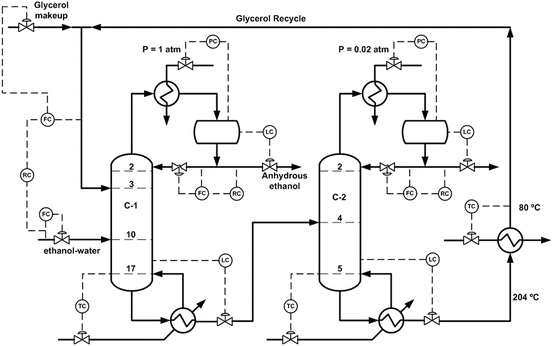

  

  Second control strategy proposed for the extractive distillation of ethanol–water mixture using glycerol as entrainer

References

Aspen Technology, Inc. (2006) Aspen HYSYS 2006: tutorials & applications. Aspen Technology, Cambridge
Chien IL, Fruehauf PS (1990) Consider IMC tuning to improve controller performance. Chem Eng Prog 86:33–41
Chien IL, Wang CJ, Wong DSH (1999) Dynamics and control of a heterogeneous azeotropic distillation column: conventional control approach. Ind Eng Chem Res 38:468–478
Fruehauf P, Mahoney D (1993) Distillation column control design using steady state models: usefulness and limitations. ISA Trans 32(2):157–175
Grassi VG (1993) Process design and control of extractive distillation, Practical distillation control. Van Nostrand Reinhold, New York, pp 370–404
Hurowitz S, Anderson J, Duvall M, Riggs J (2003) Distillation control configuration selection. J Process Control 13:357–362
Luyben WL (2002) Plantwide dynamic simulators in chemical processing and control, Chemical industries series. Marcel Dekker, New York
Luyben WL (2006) Evaluation of criteria for selecting temperature control trays in distillation columns. J Process Control 16:115–134
Luyben WL (2008) Comparison of extractive distillation and pressure-swing distillation for acetone-methanol separation. Ind Eng Chem Res 47(8):2696–2707
Perry R (1992) Chemical engineer’s handbook. McGraw-Hill, New York
Ross R, Perkins E, Pistikopoulos E, Koot G, van Schijndel J (2001) Optimal design and control of a high-purity industrial distillation system. Comput Chem Eng 25:141–150
Shinskey F (1977) Distillation control. McGraw-Hill, New York
Shinskey F (1996) Process control systems. McGraw Hill, New York
Tyreus BD, Luyben WL (1992) Tuning of PI controllers for integrator dead time processes. Ind Eng Chem Res 31:2625–2628
Author information
Authors and Affiliations
Rights and permissions
Copyright information
© 2016 Springer International Publishing Switzerland
About this chapter
Cite this chapter
Chaves, I.D.G., López, J.R.G., Zapata, J.L.G., Robayo, A.L., Niño, G.R. (2016). Dynamic Process Analysis. In: Process Analysis and Simulation in Chemical Engineering. Springer, Cham. https://doi.org/10.1007/978-3-319-14812-0_8
Download citation
DOI: https://doi.org/10.1007/978-3-319-14812-0_8
Publisher Name: Springer, Cham
Print ISBN: 978-3-319-14811-3
Online ISBN: 978-3-319-14812-0
eBook Packages: Chemistry and Materials ScienceChemistry and Material Science (R0)