Reliability-Constrained Optimal Distribution System Reconfiguration

Abstract

This work describes a method for reliability improvement of power distribution system via feeder reconfiguration. The work presented here is developed based on a linearized network model in the form of DC power flow and linear programming model in which current carrying capacities of distribution feeders and real power constraints have been considered. The optimal open/close status of the sectionalizing and tie-switches are identified using an intelligent binary particle swarm optimization based search method. The probabilistic reliability assessment is conducted using a method based on higher probability order approximation. Several case studies are carried out on a 33 bus radial distribution system and also on 118 buses large-scale distribution system, which are extensively used as examples in solving the distribution system reconfiguration problem. Further, the effect of embedded generation on distribution system reconfiguration has been considered in one case scenario. The test results show that the amount of annual unnerved energy and customer’s interruptions can be significantly reduced using the proposed method. Further, the reliability assessment method and the search method proposed in this work have both shown to be computationally efficient and very suitable for reliability-constrained feeder reconfiguration problems.

1 Introduction

The vast majority of power distribution systems are characterized by radial topological structure and poor voltage regulation. The radial topology is necessary in order to facilitate the control and coordination of the protective devices used at the distribution system level. However, with that radial structure, the failure of any single component between the load point and the source node would cause service interruptions and may result in disconnecting several load points. Distribution system reconfiguration can be used to minimize the duration and frequency of service interruptions; and thereby improving the reliability of the system and the quality of service. Distribution system reconfiguration aims at changing the topological structure of the distribution network by altering the open/close status of sectionalizing and tie-switches to achieve certain objectives. The common objective function used in distribution system reconfiguration is distribution system loss reduction and load balancing [2, 8, 9, 16, 21, 22].

In recent years, there has been an increasing interest in improving distribution system reliability using distribution system reconfiguration. The expected energy not supplied (EENS), expected demand not supplied (EDNS), and the expected outage cost (ECOST) are some examples of the reliability measures used in the literature. In Bin et al. [25] reliability worth enhancement based distribution system reconfiguration is proposed. Further, analytical and heuristic methods have been proposed for reliability worth enhancement. A reliability cost-worth model of the distribution system is built up and from which the ECOST and the EENS are obtained. In Bin et al. [25], the interrupted energy assessment rate (IEAR), which is proposed by Goel and Billinton [12] has also been used in Bin et al. [25] to relate the interruption cost and the expected energy not supplied for every feasible configuration.

A distribution system reconfiguration for reliability worth analysis based on simulated annealing is proposed in Skoonpong and Sirisumrannukul [23]. The work reported in Skoonpong and Sirisumrannukul [23] used the same reliability indices and the same customer damage function as in Bin et al. [25]. However, several conclusions about the final system configuration are drawn as the ECOST and the EENS were both considered as objectives in the optimization problem. Reliability improvement of power distribution systems using distributed generation has also been proposed in the literature [18, 24].

Swarm intelligence optimization methods or meta-heuristic methods have been widely used in distribution system reconfiguration for reliability enhancement. Amongst these methods, particle swarm optimization (PSO) based methods are recognized as viable tools in solving the distribution system reconfiguration problem for reliability improvement. The advantages of using particle swarm optimization in handling the distribution system reconfiguration problem are manifold. For instance, the status of sectionalizing and tie-switches in the distribution system can be easily represented as binary numbers of (0, 1). Moreover, particle swarm optimization based methods have considerably fast convergence characteristics and, generally speaking, have few parameters to tune up compared to some other meta-heuristic approaches. Further, particle swarm optimization has two main parameters, which are the personal best and the global best. Every particle in the swarm remembers its own personal best and at the same time its global best. Consequently, PSO based methods have more memory capability than some other swarm intelligence based methods.

Chakrabarti et al. presented a reliability based distribution system reconfiguration method in Chakrabarti et al. [6]. The objective in this study was to minimize the loss of load expectation (LOLE) and the loss of energy expectation (LOEE). Monte Carlo simulation and particle swarm optimization have also been used as searching tools. Amanulla el al. [1] proposed a reconfiguration method for large systems based on minimal cut set method. The problem of optimal switch placement in power distribution systems has been carried out using trinary PSO in Moradi and Firuzabad [19]. The use of ant colony optimization for placement of sectionalizing switches in power distribution systems has also been proposed in Falaghi et al. [11].

It is worth mentioning here that Brown [5] has reported that distribution systems contribute for up to 90 % of overall consumer’s reliability problems. This can not only be attributed to the radial topological structure of distribution systems, but also to the fact that most of nowadays distribution systems are being stressed and operated at heavily loading conditions due to the rapid increase in electricity demand and some other economical and environmental constraints. Statistics have shown also that the vast majority of consumers’ outages and service interruptions have taken place at distribution system level [3, 5]. These verities combined with the complexities of today’s distribution systems have motivated us to revamp the service of consumers by considering the reliability while reconfiguring the distribution network.

This work proposes a method for distribution system reconfiguration with an objective of reliability improvement. The work presented here is developed based on a linearized network model in the form of DC power flow model and linear programming formulation in which current carrying capacities of distribution feeders and real power constraints have been considered. The linearized network model used in this work is appropriate to use for reliability studies as it is very fast and reliable. The optimal open/close status of the sectionalizing and tie-switches are identified using an intelligent binary particle swarm optimization based search method (BPSO). The probabilistic reliability assessment is conducted using a method based on high probability order approximation. Numerous case studies are demonstrated on a small 33 bus radial distribution system and 118 buses large-scale distribution system, which have both been used as benchmark systems while solving the optimal distribution feeder reconfiguration problem. Distributed generators are constantly used in several of nowadays distribution systems. The effect of distribution generation units on the entire distribution system reliability is considered in one case study.

2 Review of Mathematical Programming Based Methods

Nonlinear optimization methods and linear optimization methods can be used for distribution system operation and planning studies. Each category has its own advantages and disadvantages. The common optimization methods applied to power distribution systems are discussed in Sect. 2.1.

2.1 Nonlinear Optimization Methods

Power systems are inherently nonlinear systems. Consequently, nonlinear optimization techniques can be used to handle power system operation and planning problems. Examples of the nonlinear optimization methods, which are widely used in the literature include, nonlinear programming, quadratic programming, and mixed-integer programming.

In nonlinear programming based optimization, both the objective function and the constraints are nonlinear. In order to handle a nonlinear programming problem, we usually start by choosing a search direction, which is obtained by finding the reduced gradient or the first derivative of the objective function. A key advantage of using nonlinear programming techniques in distribution system operation and planning studies is partly attributed to their ability to achieve higher accuracy. However, the main disadvantage of nonlinear programming based methods is that slow convergence rate may occur, which makes these methods computationally expensive, especially for applications in which repetitive solutions are required such as reliability assessment of power system, for instance. In addition, for a specific type of engineering applications the objective function can be non-differentiable. This in turn could limit the use of the nonlinear programming based methods in handling certain objective functions.

Quadratic programming can in fact be considered as a special case of nonlinear programming based technique. That is, in quadratic programming the objective function is a quadratic while the constraints are linear. A common objective function used in power system operation and planning is to minimize the total generation cost or total emission, which is inherently a quadratic function. The quadratic programming handles this problem efficiently, however, at the same time, the computational burden is considerably large. More prominently, the standard simple form of the quadratic programming is not quite often used because convergence is not always guaranteed.

Nonlinear optimization problems can also be formulated as a mixed-integer programming using certain integer control variables. Handling optimization problems using mixed-integer programming based techniques are extremely computational demanding, especially for large-scale systems.

2.2 Linear Optimization Methods

Linear methods are used to transform nonlinear optimization problems to linear problems. In this context, linear programming (LP) is probably the most popular technique, which has been widely used to handle engineering applications that require repetitive, prompt, and multiple solutions. Unlike nonlinear programming based methods, both the objective function and constraints are linear functions in the LP model. The advantages of using LP based methods in distribution system operation and planning include [27]:

• 1. Reliability of the optimization and flexibility of the solution.

• 2. Rapid convergence characteristics and fast execution time.

• 3. Nonlinear convex curves can be handled using piecewise linear models.

• 4. Equality and inequality constraints can be equally handled in the basic LP routine.

Now, suppose we have $m$ constraints with $n$ variables, the matrix of the coefficients of the constraints would be of the form [27].

$$A = \left( {\begin{array}{*{20}c} {\begin{array}{*{20}c} {a_{11} } & {a_{11} } \\ \end{array} \begin{array}{*{20}c} \ldots & {a_{1n} } \\ \end{array} } \\ {\begin{array}{*{20}c} {a_{11} } & {a_{11} } \\ \end{array} \begin{array}{*{20}c} \ldots & {a_{2n} } \\ \end{array} } \\ {\begin{array}{*{20}c} { \vdots } & \vdots \\ \end{array} \begin{array}{*{20}c} { \vdots } & \vdots \\ \end{array} } \\ {\begin{array}{*{20}c} {a_{m1} } & {a_{m1} } \\ \end{array} \begin{array}{*{20}c} \ldots & {a_{mn} } \\ \end{array} } \\ \end{array} } \right)$$

(1)

The right hand side vector b of the constraints consists of m constants,

$$b = (b_{1} ,b_{2} , \ldots ,b_{m} )^{T}$$

(2)

The row vector of the objective function c consists of n coefficients

$$c = \left( {c_{1} ,c_{2} , \ldots ,c_{n} } \right)^{T}$$

(3)

The standard maximum linear programming problem can be formulated as follows,

$$\hbox{max} (Z) = \mathop \sum \limits_{j = 1}^{n} c_{j} x_{j}$$

(4)

Subject to the following constraints,

$$\left\{ {\begin{array}{*{20}l} {\mathop \sum \limits_{j = 1}^{n} a_{ij} x_{j} \le b_{i} } \hfill \\ {x_{j} \ge 0 } \hfill \\ \end{array} } \right.$$

(5)

If the slack variables of Eq. (5) are imported, the standard linear programming will have the following form,

$$\hbox{max} \,Z = CX$$

(6)

With the equality constraints,

$$\left\{ {\begin{array}{*{20}l} {AX = b} \hfill \\ {X \ge 0} \hfill \\ \end{array} } \right.$$

(7)

The dual of this standard maximum problem is the standard minimum problem, that is,

$${\text{Min}}(W) = \mathop \sum \limits_{i = 1}^{m} b_{i} y_{i}$$

(8)

Subject to the following constraints,

$$\left\{ {\begin{array}{*{20}l} {\mathop \sum \limits_{j = 1}^{n} a_{ij} y_{j} \ge c_{j} } \hfill \\ {y_{i} \ge 0} \hfill \\ \end{array} } \right.$$

(9)

The optimal and feasible solution of Eq. (5), for instance, can be expressed as,

$$X_{b} = B^{ - 1} b$$

(10)

where B is the optimal basis at the optimal and feasible solution and $X_{b}$ is the basic variable subvector.

3 Review of Network Models

The structure of distribution systems has been recently changed due to certain environmental, economical, and political reasons. This change has come through the emergence of several real-time engineering applications in both operational and planning stages. Examples of these applications include sizing and placement of distributed generators, economic power dispatch of active distribution systems, feeder reconfiguration for service restoration and reliability enhancement, and so forth. It is very well known that these applications require a power flow study at the first step of the solution. Nevertheless, and not surprisingly, the vast majority of these applications require repetitive and prompt power flow solutions. Performing nonlinear power flow, on one hand, gives high calculation precision but requires a quite extensive computational burden and storage requirements. On the other hand, and more prominently, the largest part of the aforementioned applications is essentially nonlinear complex combinatorial constrained optimization problems. The formulation of the nonlinear problem, however, tends to be a tedious task and computationally cumbersome in terms of execution time, storage requirements, and programming. These verities combined with the large number of nodes, branches, and switches of distribution system will incontestably increase the complexity of the optimization problem.

The vast majority of power system optimization problems are essentially optimal power flow problems with different objectives. The total load curtailment minimization problem, for instance, is an important objective function that is used for reliability evaluation of power systems. We would like to elaborate here on this objective function, which is concerned with reliability improvement of distribution system. For every task of reliability evaluation, a power flow study is constantly performed. Toward this end, three power flow models have generally been used for reliability evaluation of power systems. These models are the nonlinear power flow model, the capacity flow model, and the DC power flow model. Experience with the nonlinear power flow model has shown, however, that when this model is incorporated in the reliability assessment framework, the task of reliability evaluation becomes extremely complex and oftentimes computationally intractable. Also, the required data and storage both become high. On the other hand, the capacity flow model only uses the capacity constraints of the tie-lines, and thereby; generally speaking, it is not applicable for every reliability study. In view of these reasons, in many cases, it has been found to be more appropriate to utilize the DCPF model.

The DC power flow method, which was devised more than 35 years ago, has been widely utilized in reliability assessment of power and distribution systems [17, 20]. It is denoted as DC power flow (DCPF), in analogy to a DC circuit fed by a DC voltage source. In fact, this model is a linearized version of the nonlinear power flow model; however it ignores most of the aspects of the nonlinear power flow model. The DCPF model is non-iterative, linear, and absolutely convergent, but with less accuracy than the nonlinear power flow model. The DCPF model assumes flat voltage profiles at all buses and lossless transmission lines. It is usually used whenever fast power flow solutions are required as in optimal economic power dispatch, contingency analysis, and reliability and security assessment. The DCPF model is unquestionably a powerful computational tool and was approximately involved in numerous power system operational and planning studies because of its simplicity of formulation and implementation.

It is worth to point out here that the use of the DCPF model in certain reliability evaluation studies of distribution systems has been based on the assumption that adequate information about reactive power flow are unavailable in advance. Such an assumption is justified for several planning studies because reactive power is usually supplied in a form of capacitor banks, which can be treated as a separate optimization problem.

4 Problem Statement

Distribution systems are equipped with sectionalizing and tie-switches. The crucial purpose of the tie-switches is to transfer loads from one feeder to another during abnormal and emergency conditions. The problem being presented in this work can be stated as follows: Given the distribution network with $N_{T} \in N_{TN}$ tie-switches, where $N_{TN}$ is the number of tie-switches in the distribution system, and $N_{S} \in N_{SN}$ sectionalizing switches, where $N_{SN}$ is the number of sectionalizing switches in the distribution system. The solution of the optimal distribution system reconfiguration problem $(\Omega )$ aims at finding the best combination of the tie-switches and sectionalizing switches $\Omega \in (N_{TN} \cup N_{SN} )$ that minimizes the expected power not supplied, and thereby, maximizes the overall reliability of the distribution system.

5 Development of Models and Methods

In this section, the state space of the problem is defined. Probabilistic reliability models for various distribution system components are reviewed. In addition, a reliability evaluation method based on higher probability order is introduced and discussed.

5.1 The State Space of the Problem

The state space in this work represents the set of all possible combinations of generators, distribution feeders, sectionalizing switches, tie-switches, buses, circuit breakers, and distribution transformers. Consequently, the dimension of the state space can be stated as the set of all the aforementioned components. As was mentioned earlier, distribution systems are reconfigured radially for best control of their protective relays and instruments. Therefore, the substation bus is assumed to be perfectly reliable due to the radial topological structure of the realistic power distribution systems. Modeling of these components is addressed in the subsequent section.

5.2 Distribution System Modeling

For distribution system reliability studies, probabilistic modeling techniques are utilized to represent various system components. The availability of any component $i$ in the system can be represented as [3].

$$P_{i} = \frac{{{\raise0.7ex\hbox{$1$} \!\mathord{\left/ {\vphantom {1 {\lambda_{i} }}}\right.\kern-0pt} \!\lower0.7ex\hbox{${\lambda_{i} }$}}}}{{{\raise0.7ex\hbox{$1$} \!\mathord{\left/ {\vphantom {1 {\lambda_{i} }}}\right.\kern-0pt} \!\lower0.7ex\hbox{${\lambda_{i} }$}} + {\raise0.7ex\hbox{$1$} \!\mathord{\left/ {\vphantom {1 {\mu_{i} }}}\right.\kern-0pt} \!\lower0.7ex\hbox{${\mu_{i} }$}}}}$$

(11)

where $\lambda_{i}$ is the failure rate of component $i$ and $\mu_{i}$ is the repair rate of component $i$, respectively.

In the work presented here, it is assumed that each component in the system can only reside in an up-state or down-state. Therefore, the two-state Markovian model shown in Fig. 1 is used to model various system components [3, 5]. For distribution feeders, a discrete probability density function is constructed for every distribution line. If a distribution feeder is tripped off for certain system state, the line is removed from the bus admittance matrix and its capacity is set equal to zero.

Fig. 1

Two-state Markovian model

5.3 Reliability Indices

Reliability of distribution system can be defined as the ability of the distribution system to satisfy its consumers load demand under certain operating conditions. This work uses the expected power not supplied (EPNS), which is alternatively known as the expected demand not supplied (EDNS) is used to evaluate distribution system reliability. The loss of load probability (LOLP) is used to calculate the total load curtailment $(C)$. These indices are defined as,

Expected Energy Not Supplied (EPNS): The expected number of megawatt per year that the system cannot supply to consumers. Alternatively, it is also known as the expected demand not supplied (EDNS).

Loss of Load probability (LOLP): The probability that the system will not be able to supply the load demand under certain operating scenarios.

5.4 Reliability Evaluation

Enumeration all events to compute the exact values of probabilities can sometimes be unnecessary and impractical. In practice, probabilities of occurrence of various events are approximated up to certain level. This work uses a reliability assessment method based on higher probability order approximation [4, 7]. This concept is well represented in Chen and McCalley [7] and is discussed here for the sake of completion.

Suppose we have three events, which are represented as $E_{1}$, $E_{2}$, and $E_{3}$ with individual probabilities of $P_{1}$, $P_{2}$, and $P_{3}$, respectively. The compound probability of the event $(E_{1} \cap E_{2} ) \cup E_{3}$, for instance, can be expressed as,

$$(E_{1} \cap E_{2} ) \cup E_{3} = P_{3} + P_{1} \times P_{2} - P_{1} \times P_{2} \times P_{3}$$

(12)

As can be seen from (12) this compound probability consists of first-order probability, second-order probability, and third-order probability. It is worth pointing out here that the probability of failure of most power system components is quite small. Having said that, the effect of higher-order contingencies could possibly be limited using certain probability or frequency criterion. For instance, in (2) if the individual probabilities $P_{1}$, $P_{2}$, and $P_{3}$ are quite small, then the event $(E_{1} \cap E_{2} ) \cup E_{3}$ can be approximated with $(P_{3} + P_{1} \times P_{2} )$ or with $(P_{3} )$ [7]. The reliability evaluation method followed in this work is developed based on the high probability order approximation so that the effect of any contingency level with a frequency of occurrence less than $10^{ - 10}$ has been neglected. This would in turn enhance the computational speed, without significant effect on the degree of accuracy of the estimated indices. We have shown through simulations that this method is tremendously appropriate to use for reliability evaluation studies as it is flexible and computationally efficient.

6 Reliability Evaluation Using Linearized Network Model and Linear Programming

This section formulates the optimal distribution system reconfiguration problem. It first presents the objective function and constraints. Then, it introduces a method to impose the radial topological structure of the distribution system. It also presents a method to calculate the reliability index, which is used in this work.

6.1 Objective Function

A linear Programming formulation, which is similar to similar to that given by Mitra and Singh [17], is used here to minimize total load curtailments. The equality constraints are the power flow injections at each bus, which are represented by the power balance equations. The inequality constraints include the capacity limits of generating units and power carrying capacities of distribution feeders.

The objective function used in this work can be posed as [17],

$$Loss\,of\,Load = min\mathop \sum \limits_{i = 1}^{{N_{B} }} C_{i}$$

(13)

Subject to,

$$\begin{array}{*{20}c} {\hat{B}\theta + G + C = D} \\ { G \le G^{ \hbox{max} } } \\ {C \le D} \\ { b\hat{A}\theta \le F_{f}^{ \hbox{max} } } \\ { - b\hat{A}\theta \le F_{r}^{ \hbox{max} } } \\ {G \ge 0} \\ {C \ge 0} \\ {\theta \, is\, unrestricted } \\ \end{array}$$

(14)

Where,

$N_{B}$ :

Number of buses

$N_{F}$ :

Number of distribution feeders

$\hat{B} = (N_{B} \times N_{B} )$ :

Augmented-node susceptance matrix

$b = (N_{F} \times N_{F} )$ :

Distribution feeders susceptance matrix

$\hat{A} = (N_{F} \times N_{B} )$ :

Element-node incidence matrix

$\theta = N_{B}$ :

Vector of node voltage angles

$C = N_{B}$ :

Vector of bus load curtailments

$D = N_{B}$ :

Vector of bus demand

$G^{max} = N_{B}$ :

Vector of available generation

$F_{f}^{max} = N_{F}$ :

Vector of forward flow capacities of lines

$F_{r}^{max} = N_{F}$ :

Vector of reverse flow capacities of lines

$G = N_{B}$ :

Vector of dispatched generation at buses

In (13) all generation availability and network constrains have been taken into considerations. In addition, in order to get a feasible solution for this standard minimization problem given in (13), it was assumed that one of the bus angles in (14) is considered to be equal to zero.

6.2 Imposing of the Radial Topology Constraint

Distribution systems are reconfigured radially to facilitate the control and coordination of their protective devices. The radial topological structure of the distribution system is taken as a necessary condition during the realization of the presented work. Therefore, this spanning tree structure shall be retained at all times and for all possible configurations. For this purpose, another constraint, which is developed based on graph theory [10, 13] is introduced into the distribution system reconfiguration problem. Using graph theory and the element-node incidence matrix, this constraint can be imposed as,

$${ \det }(A) = \left\{ {\begin{array}{*{20}l} { \pm 1,\,Radial\,Toplogy} \hfill \\ {0,\,Weakly - Meshed} \hfill \\ \end{array} } \right.$$

(15)

Therefore, for any optimal network configuration that results in presenting at least one loop in the system this configuration is considered to be infeasible and is removed from the search space.

To better understand the spanning tree algorithm developed herein, let us consider the graph shown in Fig. 2 [10, 13]. This graph consists of 4 vertices and 5 edges. The incidence matrix described this graph has one column of each vertex and one row for each edge of the graph. Let us draw our attention to the loop forms by the vertices 1, 2, and 3 and the edges 1, 2, and 3. The matrix describes these vertices and edges can be represented as,

$$A = \left[ {\begin{array}{*{20}c} { - 1} & 1 \\ 0 & { - 1} \\ { - 1} & 0 \\ \end{array} \begin{array}{*{20}c} 0 & 0 \\ 1 & 0 \\ 1 & 0 \\ \end{array} } \right]$$

(16)

Fig. 2

A graph with n = 4 vertices and m = 5 edges

The determinant of the incidence matrix given in (16) is obviously equal to zero. This is evident from (16) as the summation of the first two rows yields to the third row. This, in other words, indicates that the matrix described by (16) is linearly dependent. The number of loops in the graph shown below in Fig. 2 is in this case equal to 2.

6.3 Calculation of the EPNS Reliability Index

The reliability index utilized in this paper is the expected power not supplied EPNS. It is evident that (14) is augmented by a fictitious generator that is equivalent to the required curtailment since the problem aims at minimizing the total load curtailment. In this work, the EPNS is estimated as,

$$EPNS = \mathop \sum \limits_{x = 1}^{{N_{c} }} LOL(x) \times Prob(x)$$

where $LOL(x)$ is the loss of load of state $x$, which is equivalent to load curtailment of state $x$, $Prob(x)$ is the probability of state $x$, and $Nc$ is the number of contingencies.

7 Formulation of the Distribution System Reconfiguration Problem

7.1 Particle Swarm Optimization

Particle swarm optimization is a population-based optimization technique inspired by the social behavior of flocks of birds or schools of fish, which is described in detail in Kennedy and Eberhart [14, 15]. In p Particle swarm optimization, the positions and velocities of the particles are initialized with a population of random feasible solutions and search for optima by updating generations. The advantages of using particle swarm optimization technique in distribution system reconfiguration studies include the following:

• 1. Particle swarm based optimization only needs few parameters to tune up, unlike some other swarm intelligence such as genetic algorithms, for instance.

• 2. Distribution systems are equipped with two kinds of switches. These switches are sectionalizing switches and tie-switches. The sectionalizing switches are normally closed and used to connect various distribution feeders segments. On the other hand, the tie-switches are normally opened and used to transfer loads during abnormal and emergency conditions. These switches can be better represented by digital numbers 0 and 1, which are easy to implement using binary particle swarm optimization.

• 3. More prominently, as will be seen later, the PSO has two main parameters, which are the personal or individual best and the group best. Every particle in the swarm remembers its own personal best and at the same time its global best. Consequently, PSO based methods have more memory capability than some other swarm intelligence based methods such as genetic algorithms, for example.

• 4. Particle swarm optimization can handle nonlinear and non-differentiable functions efficiently and effectively.

• 5. Particle swarm optimization could lead to optimal or semi-optimal global solution for wide range of practical problems.

In PSO, the movement of the particles, which represents the potential solutions, is governed by the individual best and the group best. Using these components, a vector that determines the direction and magnitude of each particle in the swarm can therefore be represented as,

$$v_{i} = v_{i - 1} + k_{1} \times rand\left( {0,1} \right) \times \left( {P_{pbesti} - x_{i} } \right) + k_{2} \times rand\left( {0,1} \right) \times \left( {P_{gbest} - x_{i} } \right)$$

(17)

where, $rand\left( {0,\,1} \right)$ is a uniformly distributed random number between (0, 1), $P_{pbesti}$ is the particle best position from the probability of a state prospective particle $i$ has ever encountered, $P_{gbest}$ is the group of particles best position from the probability of a state prospective the group has ever encountered. Further, $k_{1}$ and are $k_{2}$ are acceleration factors. The values of these acceleration factors are given in Table 1.The change in particles positions can be defined by a sigmoid limiting transformation function and a uniformly distributed random number in (0, 1) as following,

$${\text{x}}_{\text{id}} = \left\{ {\begin{array}{*{20}l} {1, \quad rand\left( {0,\,1} \right) < S\left( {v_{id} } \right) } \hfill \\ {0,\quad otherwise} \hfill \\ \end{array} } \right.$$

(18)

where ${\text{x}}_{\text{id}}$ is the $d{\text{th}}$ component of particle $i$, and $S\left( {v_{id} } \right)$ is the sigmoid function of the $d{\text{th}}$’s component of particle $i$, which can be expressed as,

$$S\left( {v_{id} } \right) = \frac{1}{{1 + e^{{\left( { - v_{id} } \right)}} }}$$

(19)

Table 1 Reliability data

Changes of probabilities are limited by the maximum velocity, which limits the ultimate probability of a bit in particle $i$ to have 0 or 1. Choosing very large or very small values for the maximum velocity can limit the chance of exploring new vectors. Therefore, a careful selection of $v_{ \hbox{max} }$ should be performed. In this work, for a flat start, we have chosen the maximum velocity to be 2.2, which makes $S\left( {v_{id} } \right)$ varies between 90 and 10 %.

7.2 Binary Particle Swarm Optimization Based an Intelligent Search Method

The main steps of the reliability evaluation and finding the optimal configuration using the BPSO based method are summarized as follows,

• 1. Initialize the positions and velocities of the particles, respectively. Particles positions are initialized using uniformly distributed random numbers; switches that are in the closed state are represented by 1’s and switches that are in the open state are represented by 0’s.

• 2. The length of a particle string equals the number of system switches. One of the particles is chosen to represent the original configuration of the system, that is, all tie-switches are in open states.

• 3. Check if there are identical particles. If so, discard the identical ones and save the rest of the particles in a temporary array vector by converting the binary numbers to decimal numbers.

• 4. Check if there are particles already exist in the database, if so, set load curtailments of the existing particles to the system peak load to decrease the chance of visiting these configurations again. Then, save the rest in the database and go to the next step.

• 5. Check the radiality condition for each particle, if the radiality condition is met, go to next step, otherwise set load curtailments of the particles that represent invalid configuration to the system peak load to decrease the chance of visiting these configurations again.

• 6. Set system parameters and update the status of the system components (sectionalizing, tie-switches, transformers, distribution feeders, circuit breakers, etc.), for every particle.

• 7. Perform reliability evaluation for each particle by solving the linear programming optimization problem for every system state to calculate the expected load curtailments for each particle.

• 8. Determine and update personal best and global best configuration based on minimum load curtailments.

• 9. Check for convergence. If the stopping criterion is met, stop; otherwise go to next step. The stopping criteria followed here is that after little iteration, if no new better configurations were discovered, terminate the algorithm.

• 10. Update particles velocities and update particles positions using and go to step 3.

The flowchart depicted in Fig. 3 shows the detailed solution procedures.

Fig. 3

Flowchart of the proposed method

8 Demonstration and Discussion

This section provides numerous case studies to validate the effectiveness of the proposed method of optimal distribution system reconfiguration for reliability improvement. In addition, this section presents and thoroughly discusses the results.

8.1 The 33 Bus Radial Distribution System Test Case

The first distribution system used in this work is a modified 33 bus radial distribution system. The 33 bus distribution system is a 12.66 kV system, which is widely used as an example in solving the distribution system reconfiguration problem [2]. The single-line diagram of the 33 bus system is depicted in Fig. 4. The total real and reactive power loads on the system are 3,715 KW and 2,300 KVAR, respectively. Load data and line data of the 33 bus radial distribution system are given in the appendix. The base values are chosen to be 12.66 kV and 100 KVA. As shown in Fig. 4, this system consists of 33 buses, 32 branches, 3 laterals, and 5 tie lines. In addition, the 33 bus system has a distribution transformer, which is connected to the substation bus. For the initial configuration, the normally opened switches (tie-lines) are {S33, S34, S35, S36, S37}, which are represented by dotted lines. The normally closed switches are denoted as S1–S32 and are represented by solid lines.

Fig. 4

33 bus distribution system

The reliability data used in this work are acquired from Amanulla et al. [1], and are given in Table 1. The reliability index used in this paper is the EPNS. The parameters of the BPSO algorithm are given in Table 2. Several case studies have been conducted on the 33 bus distribution system shown in Fig. 4. We have also considered one case scenario for the 33 bus system in the presence of distributed generation units. The results of the different case scenario are presented in Table 3 through Table 5.

Table 2 Parameters of the proposed BPSO search method

Table 3 Reliability results of the 33 bus system-case study I

8.1.1 Case Study I

In this case study the failure rates of all distribution system components such as transformer; circuit breaker, etc. are considered. Further, it is assumed that every distribution line has a sectionalizing switch. The optimal set of the sectionalizing and tie-switches that yield minimum load curtailment were {S6, S10, S13, S27, S32}.

The number of searched configuration for this case study was 4,857. However the number of the feasible configurations was 110. For comparison purposes, the proposed method of distribution system reconfiguration is first applied on the initial configuration shown in Fig. 4. The results of this case study are summarized below in Table 3.

As can be seen from Table 2 the EPNS is reduced from 10.08 kW/year, for the initial configuration to 8.49 kW/year, after reconfiguration. This is about 15.6 % reduction in the expected power not supplied.

8.1.2 Case Study II

This case study is similar to case study I except that the failure rates of sectionalizing switches and distribution feeders are also increased by 20 %. The loading conditions have also been increased by 40 %, to show the effect of the failure rates of system components on its reliability.

The optimal set of the sectionalizing and tie-switches that yield minimum load curtailment were {S7, S11, S14, S17, S27}. The number of searched configuration for this case study was 4,904. The number of the feasible configurations for this particular case was 122. The results of this case study are summarized below in Table 4.

Table 4 Reliability results of the 33 bus system-case study III

As can be seen from Table 3, the EPNS is reduced from 15.14 kW/year for the initial configuration to 12.94 kW/year after reconfiguration. This is almost 14.53 % reduction in the expected power not supplied.

8.1.3 Case Study III

This case study discusses the inclusion of distribution generation on the reliability of the distribution network. In fact, some of today’s distribution systems have certain amount of embedded generation or distributed generation. The advantages of distributed generation include total loss reduction, voltage profile improvement, peak load shaving, and reliability and security enhancement. In this case study, we assume that certain amount of power is injected to the system via distributed generation units in order to improve its overall reliability. The distributed generators used here are modeled as constant PQ nodes with negative injections. This assumption concurs with the IEEE standard 1547–2003 (IEEE standard for Interconnecting Distributed Resources with Electric Power Systems 2003) for interconnecting distributed resources with electric power systems, which emphasizes that distributed generators are not recommended to regulate bus voltages, and thereby they should be modeled as PQ nodes not PV nodes. Further, distributed generators operated at unity power factor have been assumed in this work.

In order to accommodate the penetration of the wind turbine generators in the optimization problem, the right-hand side of (14), which represents the power balance equation, is modified to include the real power injections of the distributed generation units.

It is important to highlight here that we only consider the penetration level of the distributed generation units in this work. The problem of determining the optimal locations and sizes of distributed generation units that minimizes the total load curtailment is not pertinent to the work being presented here. Further, in this case study, we have assumed a penetration level of 10 %, which is equivalent to approximately 370 kW. Therefore, two distributed generation units, each one is rated at 185 kW, are placed at bus 8 and bus 24 of the 33 bus system, respectively.

The optimal set of the sectionalizing and tie-switches that yield minimum load curtailment for this case study were {S6, S10, S13, S26, S36}. The number of searched configuration for this case study was 4,776. The number of the feasible configurations was 111. For comparison purposes, we have placed the same distributed generation units on the initial configuration shown in Fig. 4. The results of this case study are summarized in Table 5.

Table 5 Reliability results of the 33 bus system-case of distribution generation units

As can be seen from Table 5, the EPNS is reduced from 9.86 kW/year for the initial configuration to 7.71 kW/year after reconfiguration. This is about 21.8 % reduction in the expected power not supplied. It is interesting to mention here that the present of the distributed generation units has assisted in decreasing the total amount of the curtailed power as can be seen from Table 5.

8.2 The 118 Buses Large-Scale Distribution System Test Case

The proposed framework has been applied to a more complicated and realistic distribution system to validate its feasibility in such conditions. The system under consideration is an 11 kV, 118 buses large-scale radial distribution system [26]. This system consists of 117 branches and has 15 tie-lines. The results of one case scenario performed on this system are presented. The failure rates of distribution feeders are considered in this case. For the initial configuration, the EPNS has been calculated using the proposed method and was found 313 kW/year. The EPNS has been reduced to 211 kW/year after the network has been reconfigured.

9 Discussion and Concluding Remarks

A was discussed earlier, it has been reported in the literature that distribution systems contribute for up to 90 % of overall consumer’s reliability problems [5]. Statistics have shown also that the vast majority of consumers’ outages and service interruptions have taken place at distribution system level [3, 5]. In addition, most of nowadays distribution systems are being stressed and operated at heavily loading conditions due to the rapid increase in electricity demand and some other economical and environmental constraints. These verities combined with the complexities of nowadays distribution systems have motivated us to revamp the service of consumers by considering the reliability while reconfiguring the distribution network.

Distribution systems are equipped with two types of switches; sectionalizing and tie-switches. The sectionalizing switches are normally closed and are used to connect various distribution line segments. The tie-switches, on the other hand, are normally opened and can be used to transfer loads from one feeder to another during abnormal and emergency conditions. Feeder reconfiguration is among the several operational tasks, which are performed frequently on distribution systems. Basically, it denotes to the process of changing the topological structure of the distribution network by altering the open/close status of sectionalizing and tie-switches to achieve certain objectives. Of these objectives reliability and security enhancement are of most concern.

This work has proposed a method for reliability maximization of distribution systems through feeder reconfiguration. This method is developed based on a linearized network model in which the current carrying capacities of distribution feeders and real power limits have been accounted for. From practical perspective, distribution systems are reconfigured radially for best control and coordination of their protective devices. We have therefore developed an algorithm based on the graph theory of trees and forests to preserve the radial topology constraints. Since the time and computational effort spent in evaluating reliability indices are of great concern in both planning and operational stages, this paper uses a probabilistic reliability assessment method based on event tree analysis with higher-order contingency approximation. Consequently, the computational burden has been reduced when compared to some other approaches such as Monte Carlo simulation, for instance, which sometimes tends to be computationally demanding even for planning studies.

In addition, we have proposed an intelligent binary particle swarm optimization based search method to seek the possible combinations of sectionalizing and tie-switches that improve system’s reliability. We have demonstrated the effectiveness of the proposed method on a 33-bus radial distribution system, which is extensively used as an example in solving the distribution system reconfiguration problem. We have considered the effect of embedded generation in one case scenario. The test results have shown that amount of annual unnerved energy and customer’s interruptions can be significantly decreased when reliability constraints are taken into consideration while reconfiguring the distribution network.

This work proposes a method for distribution system reconfiguration with an objective of reliability improvement. The main features of the work presented in this chapter include:

• 1. The work presented here is developed based on a linearized network model in the form of DC power flow model and linear programming formulation in which current carrying capacities of distribution feeders and real power constraints have been considered.

• 2. The linearized network model used in this paper is appropriate to use for reliability studies as it is very fast and reliable.

• 3. The optimal open/close status of the sectionalizing and tie-switches are identified using an intelligent binary particle swarm optimization based search method (BPSO).

• 4. The probabilistic reliability assessment is conducted using a method based on high probability order approximation.

• 5. Numerous case studies are demonstrated on a small 33 bus radial distribution system and 118 buses large-scale distribution system, which have both been used as benchmark systems while solving the optimal distribution feeder reconfiguration problem.

• 6. Distributed generators are constantly used in several of nowadays distribution systems. The effect of distribution generation on distribution system reliability is considered in one case study (Fig. 5).

  Fig. 5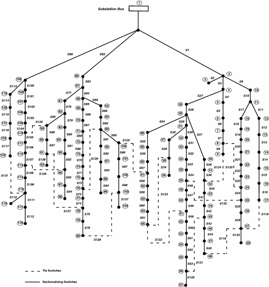

  

  118 buses distribution system

Appendix

See Tables 6 and 7.

Table 6 Line data of the 33 bus distribution system

Table 7 Load data of the 33 bus distribution system

References

Amanulla, B., Chakrabarti, S., Singh, S.: Reconfiguration of power distribution systems considering reliability and power loss. IEEE Trans. Power Del. 27(2), 918–926 (2012)
Baran, M., Wu, F.: Network reconfiguration in distribution systems for loss reduction and load balancing. IEEE Trans. Power Del. 4(2), 1401–1407 (1989)
Billinton, R., Allan, R.: Reliability Evaluation of Power Systems, 2nd edn. Plenum, New York (1996)
Billinton, R., Kumar, S.: Effect of higher-level independent generator outages in composite-system adequacy evaluation. IEEE Proc. 134(1), 17–26 (1987)
Brown, R.: Electric Power Distribution Reliability. Marcel Dekker Inc., New York City (2002)
Chakrabarti, S., Ledwich, G., Ghosh, A.: Reliability driven reconfiguration of rural power distribution systems. In: Proceedings of 3rd International Conference on Power Systems, pp.1–6, (2009)
Chen, Q., McCalley, J.: Identifying high risk N-k contingencies for online security assessment. IEEE Trans. Power Syst. 20(2), 823–834 (2005)
Chiang, H., Jean-Jumeau, R.: Optimal network reconfigurations in distribution systems. II. Solution algorithms and numerical results. IEEE Trans. Power Del. 5(3), 1568–1574 (1990)
Civanlar, S., Grainger, J., Yin, H., Lee, S.: Distribution feeder reconfiguration for loss reduction. IEEE Trans. Power Del. 3(3), 1217–1223 (1988)
Diestel, R.: Graph Theory. Elec. Ed. Springer, New York (2000)
Falaghi, H., Haghifam, M., Singh, C.: Ant colony optimization based method for placement of sectionalizing switches in distribution networks using a fuzzy multi–objective approach. IEEE Trans. Power Del. 24(1), 268–276 (2009)
Goel, L., Billinton, R.: Determination of reliability worth for distribution system planning. IEEE Trans. Power Del. 9(3), 1577–1583 (1994)
Graph Matrices.: Available online at: http://www.compalg.inf.elte.hu/tony/Oktatas/TDK/FINAL/Chap,.PDF. IEEE Standard for Interconnecting Distributed Resources with Electric Power systems, IEEE Std., 1547–2003, pp. 1–16 (2010)
Kennedy, J., Eberhart, R.: Particle swarm optimization. IEEE International Conference on Neural Networks, pp. 1942–1948 (1995)
Kennedy, J., Eberhart, R. (1997). A discrete binary version of the particle swarm algorithm. IEEE International Conference on Computational Cybernetics and Simulation, pp. 4104–4108
Merlin, A., Back, H.: Search for minimum loss operating spanning tree configuration in an urban power distribution system. In: Proceedings of 5th Power Systems Computing Conference Cambridge, U.K., pp. 1–18, (1975)
Mitra, J., Singh, C.: Incorporating the DC load flow model in the decomposition-simulation method of multi-area reliability evaluation. IEEE Trans. on Power Syst. 11(3), 1245–1254 (1996)
Mitra, J.: Application of computational Intelligence in optimal expansion of distribution systems. In: Proceedings of IEEE PES General Meeting, pp. 1–8, (2008)
Moradi, V., Firuzabad, M.: Optimal switch placement in distribution systems using trinary particle swarm optimization algorithm. IEEE Trans. Power Del. 23(1), 271–279 (2008)
Overbye, T., Cheng X., Yan S.: A comparison of AC and DC power flow models for LMP calculations. In: Proceedings 37th Annual Hawaii International Conference on Systems Science, pp. 1–9 (2004)
Rao, R., Ravindra, K., Satish, K., Narasimham, S.: Power loss minimization in distribution system using network reconfiguration in the presence of distributed generation. IEEE Trans. Power Syst., 1–9 (2012)
Shirmohammadi, D., Hong, H.: Reconfiguration of electric distribution networks for resistive line losses reduction. IEEE Trans. Power Del. 4(2), 671–679 (1989)
Skoonpong, A., Sirisumrannukul, S.: Network reconfiguration for reliability worth enhancement in distribution systems by simulated annealing. Proceedings of ECTI-CON, (2008)
Vallem, M., Mitra, J.: Siting and sizing of distributed generation for optimal microgrid architecture. In Proceedings of 37th the North American Power Symposium, pp. 611–616 (2005)
Ye Bin, Xiu-li, W., Be Zhao-hong, Xi-fan, W.: Distribution network reconfiguration for reliability worth enhancement. IEEE Conf. (1990)
Zhang, D., Fu, Z., Zhang, L.: An improved TS algorithm for loss minimum reconfiguration in large-scale distribution systems. Elect. Power Syst. Res. 77, 685–694 (2007)
Zhu, J.: Optimization of Power System Operation. Wiley-IEEE Press (2009)
Author information
Authors and Affiliations
Corresponding author
Editor information
Editors and Affiliations
Rights and permissions
Copyright information
© 2015 Springer International Publishing Switzerland
About this chapter
Cite this chapter
Elsaiah, S., Benidris, M., Mitra, J. (2015). Reliability-Constrained Optimal Distribution System Reconfiguration. In: Azar, A., Vaidyanathan, S. (eds) Chaos Modeling and Control Systems Design. Studies in Computational Intelligence, vol 581. Springer, Cham. https://doi.org/10.1007/978-3-319-13132-0_11
Download citation
DOI: https://doi.org/10.1007/978-3-319-13132-0_11
Published:
Publisher Name: Springer, Cham
Print ISBN: 978-3-319-13131-3
Online ISBN: 978-3-319-13132-0
eBook Packages: EngineeringEngineering (R0)