
Abstract
This chapter explores ways of performing a kind of commutative task by N parties, of which a particular scenario of contract signing is a canonical example. Tasks are defined as commutative if the order in which parties perform them can be freely changed without affecting the final result. It is easy to see that arbitrary N-party commutative tasks cannot be completed in less than N − 1 basic time units.
We conjecture that arbitrary N-party commutative tasks cannot be performed in N − 1 time units by exchanging less than 4N − 6 messages and provide computational evidence in favor of this conjecture. We also explore the most equitable commutative task protocols.
Access provided by Autonomous University of Puebla. Download chapter PDF
Keywords
These keywords were added by machine and not by the authors. This process is experimental and the keywords may be updated as the learning algorithm improves.
1 Introduction
This chapter explores ways of performing commutative tasks by N parties denoted \(\mathcal{A}_{0},\ldots,\mathcal{A}_{N-1}\). Tasks are defined as commutative if the order in which parties perform them can be freely changed without affecting the final result. Furthermore, another requirement is that this result is distributed among the N parties in the end.
A typical formulation, used throughout this work, is the material signature of a contract by N parties. As the contract signing protocol ends, each party obtains a printed contract bearing the N signatures of all other parties. Empty contracts can be printed by all parties. Each contract must transit through all parties to eventually bear all the required signatures.
This problem is not only of theoretical interest. Cryptography conceals the meaning of information but not its existence. In many cases network monitoring allows to infer useful information from the message flow. This attack is called traffic analysis. A well-known way to defeat traffic analysis consists in continuously padding the communication channel with dummy packets to simulate constant bandwidth occupation.
Ferguson and Schneier [1] states that “…it is very hard to hide information about the size or timing of messages. The known solutions require Alice to send a continuous stream of messages at the maximum bandwidth she will ever use…This might be acceptable for military applications, but it is not for most civilian applications…”
We also refer the reader to [2] who mentions that: “…In practice this problem has been known for a very long time, and countermeasures are routinely used in modern link encryptors, by making sure that they always send information between sender and receiver, inserting dummy information if necessary [3] . By doing so, they seek to obscure the difference between actual communication and non-communication. Unfortunately, the approach taken by link encryptors to “keep the channel full” is infeasible on the Internet, due to the requirement that the communication infrastructure serves the needs of multiple parties…”
It is hence useful to look for economical ways in which parties can exchange information without revealing their activity. Here envelopes represent constant-size encrypted data containers.Footnote 1 We show how to exchange containers between N parties in a way that ascertains that ∀i ≠ j, party \(\mathcal{A}_{i}\) can send a message to \(\mathcal{A}_{j}\) in N − 1 elementary time units, provided that the container’s capacity has not been exceeded.
Situation
N parties want to sign a contract. Signatories consider the contract valid when each party possesses a copy of the contract bearing all N genuine signatures (which can only be affixed by their respective owners). Parties are unable to meet physically, so they have to employ a postal service.
Firstly, a total of N copies with no signature must be printed, any party can print some of these empty contracts (printing doesn’t have to be done by one unique party, quite the opposite in fact).
Secondly, these copies must be sent among the parties. If at some point, party \(\mathcal{A}\) wants to send k contracts to party \(\mathcal{B}\), \(\mathcal{A}\) can put these in one single envelope and pay a postal fee for the envelope independently of its contents.
We can assume that whenever a party receives a contract it has not yet signed, the party signs it immediately. The problem consists in finding a contract signing protocol such that each contract has gone through every party at least once and such that at the end, the \(N\) contracts are distributed among the N parties.
We denote by \(\mathfrak{P}\) such a protocol.
The notation \(\mathcal{A}_{i}\mathop{ \rightsquigarrow }\limits ^{\mathit{k}}\mathcal{A}_{j}\) will mean “\(\mathcal{A}_{i}\) signs k contracts and sends them to \(\mathcal{A}_{j}\)”.
We study protocols according to the following three natural criteria:
Cost
The cost of a protocol \(\mathfrak{P}\) is the cumulated postal fee paid by all parties. We also make the assumption that this fee also does not depend on the sender and receiver, so we can consider that cost proportional to the number of envelopes sent globally (hereafter $1∕envelope).
A first natural goal consists in minimizing the postage fees \(\mathtt{Cost}(\mathfrak{P},N)\). We prove that \(\min _{\mathfrak{P}}\mathtt{Cost}(\mathfrak{P},N) = 2N - 2\).
The cheapest protocols are referred to simply as cheap protocols.
Time
In this work, we assume that transmitting an envelope takes 1 day while neglecting the administrative delay to have the contract signed once it has been received.
It is easy to see that the contract signing task cannot be completed in less than N − 1 days. We call protocols that run in N − 1 days fast protocols. If N days are allowed, reaching the $(2N − 2) cost’s lower bound is simple (e.g., protocol \(\mathfrak{P}_{\mathrm{seq}}\) in Sect. 2). Hence, we will focus our attention on the costs of fast protocols. We show how to construct some fast protocols that cost $(4N − 6) and conjecture that this cost is optimal:
Conjecture 1
For all N the cheapest fast protocol costs $(4N − 6).
We checked this conjecture for N ≤ 8 by exploiting problem symmetries and by using backtracking.
Equitableness
It is interesting to find protocols in which postage costs are distributed between parties as evenly as possible.
We observed that for 6 ≤ N ≤ 8, there exist fast protocols in which N − 6 parties pay $4 and 6 parties pay $3.
We do not know how to construct such optimally equitable protocols otherwise than by computerized search. We call such protocols equitable.
Even though current evidence that equitable protocols exist for all N is very limited, heuristics (more details are given in Sect. 10) suggest that all fast protocols are inherently inequitable in the following sense:
Conjecture 2
In every fast protocol for N parties, the most burdened party must pay $ Ω(N).
Convention
In “xxxx-protocol” the xxxx will stand for any combination of the letters F,C,E,M meaning: fast, cheap, equitable and minimal.
2 Straightforward Non-fast Protocols
A trivial sequential protocol is the following:
Note that:
-
\(\mathfrak{P}_{\mathrm{seq}}\) is not fast because \(\mathfrak{P}_{\mathrm{seq}}\) validates the contracts on day N, assuming that indexing days starts from 0.
-
\(\mathfrak{P}_{\mathrm{seq}}\) is cost optimal, i.e., \(\mathtt{Cost}(\mathfrak{P}_{\mathrm{seq}},N) = 2N - 2\).
-
\(\mathfrak{P}_{\mathrm{seq}}\) is inequitable because \(\mathcal{A}_{N-1}\) pays $(N − 1) while all other parties pay $1.
3 Graphical Representation
A protocol is entirely defined by the path followed by each contract, i.e., the sequence of \(\mathcal{A}_{i}\) s that the contracts transit through each day (one row in Fig. 1).

The matrix and the graph of \(\mathfrak{P}_{\mathrm{seq}}\)
For such a matrix to reflect a valid protocol, each \(\mathcal{A}_{i}\) must appear at least once in each row and once in the last column.
We will use a very convenient graphical representation to illustrate protocols (e.g., Fig. 1). The graph of a protocol for N parties and D days is a bidimensional graph with N × (D + 1) vertices.
Vertex (d, i) represents \(\mathcal{A}_{i}\) on day d.
An edge is drawn between (d, i) and (d + 1, j) if \(\mathcal{A}_{i}\) sends an envelope to \(\mathcal{A}_{j}\) on day d. Edges may be labeled with the number of contracts in the corresponding envelope.
Note that such graphs may not uniquely characterize a protocol (see Fig. 2).

A graph may correspond to several different protocols
4 Fast Protocols
It is easy to see that it takes at least N − 1 days to complete the contract signing process and that there is a very simple solution for doing so:
-
\(\mathfrak{P}_{\mathrm{cir}}\) is fast because \(\mathfrak{P}_{\mathrm{cir}}\) validates the contracts on day N − 1, assuming that indexing days starts from 0.
-
\(\mathfrak{P}_{\mathrm{cir}}\) is far from being cost optimal, i.e., \(\mathtt{Cost}(\mathfrak{P}_{\mathrm{cir}},N) = N(N - 1)\).
-
\(\mathfrak{P}_{\mathrm{cir}}\) is equitable because each party pays $(N − 1).
We observe that \(\mathfrak{P}_{\mathrm{cir}}\) outperforms \(\mathfrak{P}_{\mathrm{seq}}\) by one day, but this (small) improvement comes at the rather high price of a quadratic increase in postage costs.
It is hence natural to ask if linear-cost fast protocols exist and, more generally, find out what the cost \(\mathtt{CFP}(N)\) of the cheapest fast protocol is.
5 A Linear Protocol
The following protocol was designed following the intuition that to reduce costs, contracts must follow very similar routes. The obstruction to this is that each contract must carefully avoid one participant, namely, the party at which this contract’s route will end. We hence design two parallel routes with one contract jumping from one route to the other, at each step.
\(\mathtt{Cost}(\mathfrak{P}_{\mathrm{lin}},N) = 4N - 6\). The cost vector of \(\mathfrak{P}_{\mathrm{lin}}\) (fees paid by \(\{\mathcal{A}_{0},\ldots,\mathcal{A}_{N-1}\}\)) is
As mentioned previously, we conjecture $(4N − 6) to be optimal, i.e., \(\mathtt{CFP}(N) = 4N - 6\). We thus call $(4N − 6) protocols cheap protocols. The matrix and graph of a circular (resp. linear) protocol are given in Fig. 3 (resp. 4).

The matrix and the graph of \(\mathfrak{P}_{\mathrm{lin}}\)

The matrix and the graph of \(\mathfrak{P}_{\mathrm{cir}}\)
6 Counting Protocols
We denote by
6.1 Observations
Label each contract by the index of the party that will eventually own this contract; the sequence of parties that each contract n goes through in N − 1 days must be a permutation of the set \(\{\mathcal{A}_{0},\ldots,\mathcal{A}_{N-1}\}\). As such we can identify a fast protocol with an ordered set of N permutations,Footnote 2 in which the nth permutation ends with n.
Also note that for any fast protocol, on day N − 1 there will always be N envelopes sent, one to each party.
6.2 Number of Protocols
We have tried to enumerate fast protocols and look for some pattern in their numbers.
As pointed out supra, a fast protocol can be bijectively mapped to an ordered set of N permutations of \(\mathbb{S}_{N}\), \(\mathfrak{P} = (\mathfrak{P}_{0},\ldots,\mathfrak{P}_{N-1})\) where \(\mathfrak{P}_{n}(N - 1) = n\).
Using \(\mathfrak{P} = \mathfrak{P}_{\mathrm{lin}}\) in Fig. 3 as an example, the nth row \(\mathfrak{P}_{n}\) is the cycle \(\gamma (n,\ldots,N) = (0,\ldots,n - 1,n + 1,n + 2,\ldots,N,n)\).
For \(n = 0,\ldots,N - 1\), consider the nth row without its last coordinate : \((\mathfrak{P}_{n}(0),\ldots,\mathfrak{P}_{n}(N - 2))\) is a permutation of \(\mathbb{S}_{N}\setminus \{n\} \simeq \mathbb{S}_{N-1}\).
The last coordinate that was removed must be equal to the row index. Consequently, fast protocols can be bijectively mapped onto sets of N permutations of \(\mathbb{S}_{N-1}\). There are therefore ((N − 1)! )N fast protocols. Using that identification, we denote the set of fast protocols by \((\mathfrak{S}_{N-1})^{N}\).
6.2.1 Using Symmetry
There is a lot of symmetry in this problem, that we exploited to examine a (somewhat) lesser number of protocols.
The relabeling of \(\mathfrak{P}\) by a permutation \(\sigma \in \mathfrak{S}_{N}\) is the protocol obtained by renaming each party \(\mathcal{A}_{n}\) as \(\mathcal{A}_{\sigma (n)}\):
Notice that the change of index is such that \((\sigma (\mathfrak{P}))_{n}(n) = n\).
6.2.2 Protocol Isomorphism
Two protocols \(\mathfrak{P},\mathfrak{P}'\) are truly isomorphic,Footnote 3 if \(\mathfrak{P}\) can be transformed into \(\mathfrak{P}'\) by relabeling. We denote this relation by \(\mathfrak{P} \equiv \mathfrak{P}'\).
The number of number of fast protocols up to true isomorphism NFP T(N) as a function of N is currently unknown for N > 6.
A naïve algorithm for deciding if \(\mathfrak{P} \equiv \mathfrak{P}'\) requires O(N 2 ⋅ N! ) time. We will now show that the protocol isomorphism decision problemFootnote 4 can be solved in O(N 3) time.
An interesting relabeling is \(\sigma _{\mathrm{Id}} = \mathfrak{P}_{n}^{-1}\) for some \(n \in \mathbb{S}_{N}\). σ Id satisfies:
that is to say that the last ((N − 1)th) row of the relabeled matrix is the identity permutation.
And this equality holds if and only if \(\sigma _{\mathrm{Id}} = \mathfrak{P}_{n}^{-1}\) for some n.
In the lexicographical order on permutations \(\pi = (\pi (0),\ldots,\pi (N - 1))\) seen as words of length N, Id is the smallest of all permutations.
Hence, when looking at protocols, which are ordered sets of N permutations \((\mathfrak{Q}_{n})_{n=0,\ldots,N-1}\) as the concatenation \((\mathfrak{Q}_{N-1},\ldots,\mathfrak{Q}_{0})\) (this is a relation on N × N matrices observed as words of length N 2), we notice that the set \(I_{\mathfrak{P}} =\{ \mathfrak{P}_{n}^{-1}(\mathfrak{P})\,\vert \,n = 0,\ldots,N - 1\}\) contains the lexicographically smallest protocols which are isomorphic to \(\mathfrak{P}\): it is exactly the set of protocols isomorphic to \(\mathfrak{P}\) such that the last row of their matrix is Id.
Note that \(I_{\mathfrak{P}}\) does not always have cardinality N, e.g., in \(\mathfrak{P}_{\mathrm{cir}}\) illustrated in Fig. 4, \(I_{\mathfrak{P}_{\mathrm{cir}}} =\{ \mathfrak{P}_{\mathrm{cir}}\}\) is a singleton.
Furthermore, the family of sets \(I_{\mathfrak{P}}\) defines a partition of the set of matrices whose last row is the identity permutation. Each \(I_{\mathfrak{P}}\) has size at most N. And only one protocol per set is minimal in its true isomorphism class.
Hence a lower bound of the number of fast and minimal protocols is:
This is also a rough estimate of the actual number \(\mathtt{NFP}^{\mathrm{T}}(N)\), if we assume that for most protocols, informally, \(\vert S_{\mathfrak{P}}\vert \sim N\) (approximately equal). This approximation means that protocols are rarely their own relabeling by a nontrivial permutation; this indicates that the roles played by all parties are generally asymmetrical in some sense. Although limited, the current evidence shows a rather accurate lower bound.
For N = 5, we found that there are \(\mathtt{NFP}^{\mathrm{T}}(5) = 66,360\) different protocols up to isomorphism, which is pretty close to \(\frac{(4!)^{4}} {5} = 66,355.2\).
For N = 6 we get \(\mathtt{NFP}^{\mathrm{T}}(6) = 4,147,236,820 \simeq \frac{(5!)^{5}} {6} = 4,147,200,000\).
By examining only the N permutations that constitute \(\mathfrak{P}\), it is possible to determine in O(N 3) time the smallest protocol isomorphic to \(\mathfrak{P}\) (e.g., Fig. 5).

Two isomorphic protocols \(\mathfrak{P}\) (above) and \(\mathfrak{P}' =\sigma (\mathfrak{P})\) (below), where \(\sigma = \mathfrak{P}_{0}^{-1} = (4\,1\,0\,3\,2)\). \(\mathfrak{P}'\) is the lexicographically smallest protocol isomorphic to \(\mathfrak{P}\)
It is then a matter of checking equality between those single minimal representatives to decide if two protocols are isomorphic.
All in all, this process claims O(N 3) time.
6.2.3 Simple Isomorphism
Another equivalence relation can be defined by only considering the last row of every matrix, and the corresponding relabeling. Two protocols \(\mathfrak{P}\) and \(\mathfrak{P}'\) are simply isomorphic if their respective relabelings by the permutation found in the last row are equal:
Simple isomorphism is a proper subrelation of true isomorphism: two isomorphic protocols are simply isomorphic, but the converse is not always true.
However, this new relation is peculiar in that:
-
compared to true isomorphism, it is easier to tell whether a matrix is the lexicographical minimum of its simple isomorphism class, as it amounts to checking that the last row is the identity,
-
simple isomorphism classes partition the set of protocols evenly into sets of size (N − 1)! , as every class can be bijectively mapped to \(\mathfrak{S}_{N-1}\) by associating an arbitrary permutation to its last row. We can find the number of protocols with a given cost by only enumerating protocols up to simple isomorphism, and then multiplying their number by (N − 1)! . In particular, the number of fast protocols up to simple isomorphism is:
$$\displaystyle{\mathtt{NFP}^{\mathrm{S}}(N) = \frac{\mathtt{NFP}(N)} {(N - 1)!} = ((N - 1)!)^{N-1}.}$$True isomorphism does not define an even partition, in fact the number of matrices isomorphic to \(\mathfrak{P}\) is \((N - 1)! \cdot \vert I_{\mathfrak{P}}\vert \), which is not a constant.
6.2.4 Backtracking
We have designed a backtracking algorithm to enumerate all fast protocols whose costs are bounded by a certain value.
The algorithm consists in incrementally completing a partial protocol in every possible way while keeping track of a lower bound on the cost, and backtracking as soon as the upper limit is reached (e.g., when the lower bound exceeds 4N − 6).
As pointed out earlier, to enumerate matrices up to (true or simple) isomorphism, we can consider only matrices whose last row is the identity permutation, as all minimal representatives of isomorphism classes are to be found among these.
The number of such matrices is \(((N - 1)!)^{N-1}\); compared with the original ((N − 1)! )N, this saves the effort of one iterative layer over a set of permutations.
In the case of true isomorphism, when a complete protocol is obtained, we check if it is lexicographically minimal in its isomorphism class, in which case it can be processed or stored for further examination.
To prune even more possibilities, we can further exploit the fact that the protocols we are looking for need to be lexicographically minimal. For example, instead of checking minimality once the protocol has been completed, it is possible to relabel the partial protocol to see that any completion of it will not be minimal. Unfortunately, in our attempt, the resulting overhead outweighted the pruning. We assume this is due to the small values of N we could examine, and that this modification results in a faster algorithm for greater protocols.
By exhaustively examining all protocols whose last row is Id, we could enumerate all fast protocols for N ≤ 6 (Tables 1 and 2).
And using backtracking as described above, we enumerated some of the cheapest protocols for N = 7, 8 while checkingFootnote 5 that protocols cheaper than $(4N − 6) do not exist.
Table 1 also provides the number of $ c protocols for \(4N - 6 \leq c \leq N(N - 1)\).
7 Equitableness
In \(\mathfrak{P}_{\mathrm{lin}}\), all parties but one pay a fixed fee, and one party pays a fee that increases with N. This is not an equitable protocol. We hence looked for the most equitable cheap protocol.
We measure equitableness using the Theil index:
where m n is the fee paid by \(\mathcal{A}_{n}\) and
is the average fee.
A smaller \(T_{N}(\mathfrak{P})\) value expresses a more equitable protocol.
We computed the average Theil index of (fast and) cheap protocols, and we also enumerated those that are equitable with results in Tables 3 and 4.
For N = 7, the average Theil index computed over all minimal representatives of protocol isomorphism classes is ≃ 0. 077, whereas the minimum index is ≃ 0. 0058, reached by the 12 FCEM protocols given in the appendix. We also illustrate in Fig. 6 one of the 27 FCEM protocols for N = 8, found by automated search.

Equitable protocol, N = 8 of cost vector (4, 3, 3, 4, 3, 3, 3, 3) (example)
7.1 Symbol Insertion Experiments
It is natural to wonder if FCE protocols can be constructed from smaller ones. To get a hint, we took all 27 eight-party FCEM protocols \(\mathfrak{P}_{1},\ldots,\mathfrak{P}_{27}\) and performed the following exploration:

Indeed, the above algorithm detected 168 different ways to build (non necessarily minimal) eight-party FCE protocols by inserting new symbols into 7 seven-party FCEM protocols. The process is illustrated in Fig. 7.

Symbol deletion experiment (example). The deleted symbol is 0
The experiment was repeated mutatis mutandis by eliminating all possible combinations of two rows (and their corresponding pairs of symbols). There were 136 ways to obtain eight-party FCE protocols using symbol insertions into six-party FCEM protocols. Only two protocols out of the five equitable six-party protocols enabled these insertions, and 17 out of the 27 eight-party FCEM protocols could be reached that way.
Results are available online.Footnote 6
We doubt that this process would allow to infer a general process for constructing (N + 1) party FCE protocols by extending N-party FCE protocols for the following reason: for N = 6, 7, 8 all FCE protocols have four active parties on day N − 2, never 2 or 3 nor 5.
The exhaustive list of matrices for N = 6, 7, 8 hints that we cannot do better than four parties on day N − 2. If there was an algorithm allowing to build FCE protocols from smaller ones, this algorithm would have to add active parties on day N − 2, and it would be unexpected for it not to work for six, seven, or eight parties.
We regard this as evidence that the algorithmic construction of FCEM protocols is a nontrivial problem.
This approach can be used to find a way of generating cheap protocols rather than equitable protocols. Indeed, there is a pattern we have discovered, though without the use of this approach, as explained in Sect. 9.1.
8 Lower Bounds
8.1 General Case
With no conditions on the protocol’s duration D, we show that
as achieved by \(\mathfrak{P}_{\mathrm{seq}}\).
It should be noted that in general having some party hold a contract for several consecutive days without sending it away is an allowed “move,” and is of course free of charge.
Only with the now unassumed constraint of validation in N − 1 days, it becomes necessary to have all contracts circulating in envelopes every day.
The same applies as well to the fact that a contract can transit through one same party multiple times.
Proof
The proof is done by induction on the number of parties N.
When N = 1, it is clear that \(\mathtt{Cost}(\mathfrak{P},1) = 0\).
Assume that for every N-party protocol \(\mathfrak{P}'\), \(\mathtt{Cost}(\mathfrak{P}') \geq 2N - 2\). Let us prove that for every (N + 1)-party protocol, \(\mathtt{Cost}(\mathfrak{P}) \geq 2N\).
Let \(\mathfrak{P}\) be a $ c (N + 1)-party protocol.
By conveniently removing one party from \(\mathfrak{P}\), we will create an N-party protocol \(\mathfrak{P}'\) that costs at most $(c − 2).
Then, using the inductive hypothesis for \(\mathfrak{P}'\),
will conclude the inductive step.
At least one party is to print an empty copy of the contract, which will be sent using one envelope. Without loss of generality, we can assume that \(\mathcal{A}_{N}\) is one of those who print contracts, that is the party we will want to remove from this protocol.
8.1.1 A First Protocol Transformation
Instead of having \(\mathcal{A}_{N}\) print contracts (on day 0) and send them to \(\mathcal{A}_{\alpha _{0}},\mathcal{A}_{\alpha _{1}},\ldots\) (not necessarily on day 0), we will have \(\mathcal{A}_{\alpha _{0}},\mathcal{A}_{\alpha _{1}},\ldots\) print these contracts. Because \(\mathcal{A}_{N}\) is assumed to print at least one contract, at least one less envelope will be used (Fig. 8).

Transformation on day 0 (first transformation)
We now have to consider the points in time at which \(\mathcal{A}_{N}\) receives some contracts.
This must happen at least once, as every party must receive a final copy of the contract at some point.
8.1.2 A Second Protocol Transformation
The following transformation removes another envelope from the process.
-
If \(\mathcal{A}_{N}\) receives only one envelope containing only the contract that \(\mathcal{A}_{N}\) is to own, then we can just remove this envelope from the protocol.
-
Otherwise, \(\mathcal{A}_{N}\) receives some contracts which are to be signed by \(\mathcal{A}_{N}\). Then these contracts need to be rerouted away (not necessarily on the same day), excluding the contract that is ultimately bound to reach \(\mathcal{A}_{N}\) that we will just remove.
Denote by \(\mathcal{A}_{\beta _{0}},\mathcal{A}_{\beta _{1}},\ldots\) the parties those contracts will be sent to next. There must be at least one of them, \(\mathcal{A}_{\beta _{0}}\). Since \(\mathcal{A}_{N}\) is to be removed, we can change the destination of the contracts to \(\mathcal{A}_{\beta _{0}}\) instead of \(\mathcal{A}_{N}\), and one less envelope will be used as \(\mathcal{A}_{\beta _{0}}\) does not need to send a contract to himself (Fig. 9).
With the above two transformations, we can obtain an N-party protocol instead of an N + 1 one while removing at least one envelope with each transformation. Therefore the resulting protocol costs at most $(c − 2).
We can conclude that for all N-party protocols, \(\mathtt{Cost}(\mathfrak{P}) \geq 2N - 2\).

Transformation when \(\mathcal{A}_{N}\) receives envelopes (second transformation)
8.2 Fast Protocols
Although still unsatisfactory, a lower bound \(\mathtt{CFP}(N) \geq 3N - 5 +\log _{2}(N)\) can be proven.
We first prove that \(\mathtt{CFP}(N) \geq 3N - 4\).
Proof
Assume that \(\mathtt{CFP}(N) \leq 3N - 5\) for some N.
Since \(\mathtt{CFP}(2) = 2\), we can assume that N ≥ 3.
Let \(\mathfrak{P}\) be a $ CFP(N) protocol, i.e., a protocol using less than 3N − 5 envelopes.
We know that on day N − 2, exactly N envelopes are sent. Hence between days 0 and N − 3, strictly less than 2(N − 2) envelopes would be sent.
On at least one day ≤ N − 3, only one envelope is sent; therefore all contracts go through one same party, and on the last day the contract that this party receives would have gone through it twice, which is impossible.
The N contracts must follow N different paths between days 0 and N − 2, as the final destination of each contract is the only party it hasn’t gone through during days 0 to N − 2. Moreover, we can bound the number of different available paths when using \(3N - 4 + q\) envelopes by 2q+1.
Proof
We say that party \(\mathcal{A}_{n}\) is active on day d in protocol \(\mathfrak{P}\) if \(\mathcal{A}_{n}\) has at least one contract on day d, i.e., ∃k such that \(\mathfrak{P}_{k}(d) = n\).
For every active party on each day between days 1 and N − 3, choose one envelope among those sent; we call those chosen envelopes default envelopes. Also choose only one default envelope on day 0.
The number of default envelopes is equal to the cumulated number of active parties in days 1 to N − 3, plus one on day 0. That is at least 2N − 5 as a consequence of the previous proof. There are also N envelopes sent on day N − 2.
Therefore there are at most q + 1 non-default envelopes between days 0 and N − 2.
We associate any path between days 0 and N − 2 with the set L of non-default envelopes that it contains.Footnote 7 This defines an injection into the set of subsets of non-default envelopes, whose size is at most 2q+1.
The reverse procedure to recover a path Δ from its associated subset L consists in the following, starting on day 0:
-
If no envelope sent on day 0 is in L, then path Δ starts with the default envelope.
-
Otherwise there should be a unique such envelope, and this is the first envelope in the path.
The reason why we chose only one default envelope on day 0 is that we don’t know yet where the path begins from. This default envelope allows to set a default starting party at the same time.
Once the first envelope in Δ is found, Δ(0) and Δ(1) are known.
We carry on by induction. On each day \(d = 1,\ldots,N - 2\), assume that Δ(d) is known; there is at most one envelope in L which was sent on day d. If there is none, then Δ(d + 1) is the recipient of the default envelope sent by Δ(d).
A conflict in this procedure, where there are several envelopes in L among those sent on day d, means that L is not associated with any path.
This procedure shows that there are at most 2q+1 paths.
Since there must be at least N paths, q ≥ log2(N) − 1.
In conclusion,
9 Leads
Looking at the proof of the previous lower bound, it is natural to wonder whether we can improve on the lower bound of two envelopes/day.
This is however the best we can do as illustrated in Fig. 11.

On day 1, only two envelopes are sent
This example can be generalized to all N ≥ 4.
Other examples were found where only two envelopes were sent on a day other than N − 3.
9.1 A Wider Class of Protocols
Given one $(4N − 6) protocol \(\mathfrak{P}\) for N ≥ 2, such that on day 0 only two parties print empty contract copies, we can build an (N + 1)-party protocol verifying the same property.
This construction can produce the \(\mathfrak{P}_{\mathrm{lin}}\) protocol and many more cheap protocols which do not comply with the above property, starting with one smaller-size protocol.
Extend every path in protocol \(\mathfrak{P}\) by appending N at the beginning (N paths are defined that way).
Choose \(n \in \mathbb{S}_{N}\), consider the path Δ ending at n, draw a new path that begins at n, ends at N, and follows Δ in between.
This method hints that the number of $(4N − 6) protocols grows at least a fast as a factorial. Example: Fig. 12.

Extension of the protocol of Fig. 11
9.2 Another Point of View
This problem of contract signature can be equivalently formulated as a variant of the traveling salesman problem. This alternative point of view may provide more insight into the problem, although to this date it is still unclear in what way precisely.
There are N salesmen who are located at different cities at the beginning, and each of them wishes to visit all N cities while minimizing transport fees. To that end, they can cooperate by carpooling, such that if k salesmen are at the same city at the same time and if their current destinations are the same, then the overall cost of transport is the same as for 1 salesman.
This formulation amounts to looking at signing protocols in reversed time. Moreover, this point of view reveals several possible generalizations. Indeed, since in this chapter we consider that any party can send mail to any other party, this relationship can be described by a complete graph; it is then natural to wonder how the problem changes with more general classes of graphs: not necessarily complete, with weights indicating different fees or routing delays associated to different sources and destinations, etc.
However a notion such as equitableness for the parties becomes meaningless, as focus is shifted from parties/cities to contracts/salesmen, instead we can then define equitableness for the salesmen.
10 Open Questions and Further Research
Besides proving (or refuting) Conjectures 1 and 2, we encourage readers to research the following open problems:
Algorithmic Construction of FCE Protocols
If equitable protocols exist for all N, design an efficient strategy for constructing FCE protocols. Here “efficient” means constructing a protocol in O(N t) for some fixed t.
It seems there cannot be more than four “active” parties on day N − 2, whatever the protocol is. If that is true then, and because there must be N envelopes sent on this last day, one of the parties is going to pay at least $ N∕4. The best case is $ N∕4 for every four parties.
Assume on the contrary that equitable protocols exist for all N, or even a weaker form of equitableness where the individual cost is bounded by a constant C. On day N − 2, N envelopes must be sent. Since every party pays less than $ C, there are at least N∕C active parties on day N − 2, N∕C 2 on day N − 3, and so on. There would be a treelike structure at the end of the corresponding graph, which means a lot of active parties—whereas the idea behind the current minimal cost protocols is quite the opposite. When N is large enough, this takes a lot of envelopes to set up; in fact we believe that it takes too many and that there won’t be enough on the first days. But we are unsure and maybe such a tree would end up being possible.
Being able to look for equitable protocols for N = 9 would be a first step. Finding out if equitable protocols still exist for N = 12 or 13 would provide very strong evidence in favor of or against the existence of equitable protocols for all N.
Finding a Protocol Matching (or Best Matching) a Given Cost Vector
Given a cost vector:
identify the protocol \(\mathfrak{P}_{s}\) that deviates as little as possible from c.
What Are the Possible Cost Vectors?
Let \(\mathbb{P}_{N} =\{ \mathfrak{P}_{1},\ldots,\mathfrak{P}_{\mathrm{\mathtt{NCP}}(N)}\}\) be all N-party FC protocols. Let s i denote the cost vector of \(\mathfrak{P}_{i} \in \mathbb{P}_{N}\) with elements sorted by increasing order.Footnote 8 How many different s i s are there? What can be said about their frequencies?
Nonconstant Postage Fees
We assumed that the cost of an envelope is independent of the number of contracts sent. What happens for a general cost function f(k), for instance, \(f(k) = \mathit{ak} + b\) or \(f(k) = a\lceil k/b\rceil \)?
Continuous Flow Communication
This chapter dealt with a latency of N − 1 days. What happens if N − 1 shifted protocols are started simultaneously so that N − 1 protocols are always run in parallel? Here the most equitable setting would be N − 6 parties paying $(4N − 10) and six parties paying $(4N − 9) but is this achievable?Footnote 9 If so, how regular can the spending rate of each party be? (i.e., avoid sudden “spending bursts”).
If Conjecture 2 Is True
Does relaxing the fast protocol hypothesis enable equitableness?
11 Appendix: FCEM Protocols for N = 7

Notes
- 1.
\(\mathcal{A}_{i}\) gets a container, decrypts it, and examines its contents. \(\mathcal{A}_{i}\) extracts any messages sent to him and erases these messages from the container. \(\mathcal{A}_{i}\) potentially inserts into the container new messages for other parties and re-encrypts the container for the next receiving party without changing the container’s size.
- 2.
Of \(\mathbb{S}_{N}\).
- 3.
Or isomorphic when there is no ambiguity as is the case until the other relation is presented.
- 4.
That is, given \(\mathfrak{P},\mathfrak{P}' \in \mathfrak{S}_{N-1}^{N}\), decide if \(\mathfrak{P} \equiv \mathfrak{P}'\).
- 5.
Our Ocaml code is available at http://www.eleves.ens.fr/home/xia/posting.
- 6.
- 7.
The reader is referred to Fig. 10 for a clarifying example.
Fig. 10 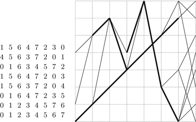
Protocol from Fig. 6 where edges representing default envelopes are drawn in thick lines
An edge \((d,\alpha ) - (d + 1,\beta )\) means that \(\mathcal{A}_{\alpha }\) sends an envelope to \(\mathcal{A}_{\beta }\) on day d.
The path (1, 5, 6, 4, 7, 2, 3) is associated to the set \(\{(0, 1) - (1, 5); (2, 6) - (3, 4); (5, 2) - (6, 3)\}\) (the final destination of the corresponding contract is \(\mathcal{A}_{0}\)).
Note that all available paths on this graph are not necessarily taken by a contract, e.g., (4, 5, 6, 4, 7, 2, 3) is associated to \(\{(0, 4) - (1, 5); (5, 2) - (6, 3)\}\).
- 8.
That is, renumbering the parties by increasing workload.
- 9.
For example, if we launch seven shifted instances of Fig. 6 we get a very uneven split of cost where \(\mathcal{A}_{0}\) and \(\mathcal{A}_{3}\) pay $4 every day (i.e., a total of $28 each) whereas the other six parties pay $3 every day (i.e., a total of $21 each).

References
N. Ferguson, B. Schneier, Practical Cryptography (Wiley, Indianapolis, 2003)
K. McCurley, Language modeling and encryption on packet switched networks, in Advances in Cryptology - Eurocrypt 2006. Lecture Notes in Computer Science, vol. 4004 (Springer, Berlin, 2006), pp. 359–372
V. Voydoc, S. Kent, Security mechanisms in high-level network protocols. ACM Comput. Surv. 15, 135–171 (1983)
Acknowledgements
The authors thank Oğuzhan Külekci for interesting discussions and useful remarks notably concerning the variant of the traveling salesmen problem.
Author information
Authors and Affiliations
Corresponding author
Editor information
Editors and Affiliations
Rights and permissions
Copyright information
© 2014 Springer International Publishing Switzerland
About this chapter
Cite this chapter
Brier, E., Naccache, D., Xia, Ly. (2014). How to Sign Paper Contracts? Conjectures and Evidence Related to Equitable and Efficient Collaborative Task Scheduling. In: Koç, Ç. (eds) Open Problems in Mathematics and Computational Science. Springer, Cham. https://doi.org/10.1007/978-3-319-10683-0_13
Download citation
DOI: https://doi.org/10.1007/978-3-319-10683-0_13
Published:
Publisher Name: Springer, Cham
Print ISBN: 978-3-319-10682-3
Online ISBN: 978-3-319-10683-0
eBook Packages: Computer ScienceComputer Science (R0)