Propositional Encoding of Constraints over Tree-Shaped Data

Abstract

We present a functional programming language for specifying constraints over tree-shaped data. The language allows for Haskell-like algebraic data types and pattern matching. Our constraint compiler CO4 translates these programs into satisfiability problems in propositional logic. We present an application from the area of automated analysis of termination of rewrite systems, and also relate CO4 to Curry.

This author is supported by an ESF grant.

These keywords were added by machine and not by the authors. This process is experimental and the keywords may be updated as the learning algorithm improves.

1 Motivation

The paper presents a high-level declarative language CO4 for describing constraint systems. The language includes user-defined algebraic data types and recursive functions defined by pattern matching, as well as higher-order and polymorphic types. This language comes with a compiler that transforms a high-level constraint system into a satisfiability problem in propositional logic. This is motivated by the following.

Constraint solvers for propositional logic (SAT solvers) like Minisat [ES03] are based on the Davis-Putnam-Logemann-Loveland (DPLL) [DLL62] algorithm and extended with conflict-driven clause learning (CDCL) [SS96] and preprocessing. They are able to find satisfying assignments for conjunctive normal forms with $10^6$ and more clauses in a lot of cases quickly. SAT solvers are used in industrial-grade verification of hardware and software.

With the availability of powerful SAT solvers, propositional encoding is a promising method to solve constraint systems that originate in different domains. In particular, this approach had been used for automatically analyzing (non-)termination of rewriting [KK04, ZSHM10, CGSKT12] successfully, as can be seen from the results of International Termination Competitions (most of the participants use propositional encodings).

So far, these encodings are written manually: the programmer has to construct explicitly a formula in propositional logic that encodes the desired properties. Such a construction is similar to programming in assembly language: the advantage is that it allows for clever optimizations, but the drawbacks are that the process is inflexible and error-prone.

This is especially so if the data domain for the constraint system is remote from the “sequence of bits” domain that naturally fits propositional logic. In typical applications, data is not a flat but hierarchical (e.g., using lists and trees), and one wants to write constraints on such data in a direct way.

Therefore, we introduce a constraint language CO4 that comes with a compiler to propositional logic. Syntactically, CO4 is a subset of Haskell [Jon03], including data declarations, case expressions, higher order functions, polymorphism (but no type classes). The advantages of re-using a high level declarative language for expressing constraint systems are: the programmer can rely on established syntax and semantics, does not have to learn a new language, can re-use his experience and intuition, and can re-use actual code. For instance, the (Haskell) function that describes the application of a rewrite rule at some position in some string or term can be directly used in a constraint system that describes a rewrite sequence with a certain property.

A constraint programming language needs some way of parameterizing the constraint system to data that is not available when writing the program. For instance, a constraint program for finding looping derivations for a rewrite system $R$, will not contain a fixed system $R$, but will get $R$ as run-time input.

A formal specification of compilation is given in Sect. 2, and a concrete realization of compilation of first-order programs using algebraic data types and pattern matching is given in Sect. 3. In these sections, we assume that data types are finite (e.g., composed from Bool, Maybe, Either), and programs are total. We then extend this in Sect. 4 to handle infinite (that is, recursive) data types (e.g., lists, trees), and partial functions. Note that a propositional encoding can only represent a finite subset of values of any type, e.g., lists of Booleans with at most 5 elements, so partial functions come into play naturally.

We then treat in Sect. 5 briefly some ideas that serve to improve writing and executing CO4 programs. These are higher-order functions and polymorphism, as well as hash-consing, memoization, and built-in binary numbers.

Next, we give an application of CO4 in the termination analysis of rewrite systems: In Sect. 6 we describe a constraint system for looping derivations in string rewriting. We compare this to a hand-written propositional encoding [ZSHM10], and evaluate performance. The subject of Sect. 7 is the comparison of CO4 to Curry [Han13], using the standard $N$-Queens-Problem as a test case.

Our constraint language and compiler had been announced in short workshop contributions at HaL 8 (Leipzig, 21 June 13), and Haskell and Rewriting Techniques (Eindhoven, 26 June 13). The current paper is extended and revised from our contribution to Workshop on Functional and Logic Programming (Kiel, 11 September 13). Because of space restrictions, we still leave out some technicalities in Sects. 2 and 3, and instead refer to the full version [BW13].

2 Semantics of Propositional Encodings

In this section, we introduce CO4 syntax and semantics, and give the specification for compilation of CO4 expressions, in the form of an invariant (it should hold for all sub-expressions). When applied to the full input program, the specification implies that the compiler works as expected: a solution for the constraint system can be found via the external SAT solver. We defer discussion of our implementation of this specification to Sect. 3, and give here a more formal, but still high-level view of the CO4 language and compiler.

Evaluations on Concrete Data. We denote by $\mathbb {P}$ the set of expressions in the input language. It is a first-order functional language with algebraic data types, pattern matching, and global and local function definitions (using let) that may be recursive. The concrete syntax is a subset of Haskell. We give examples— which may appear unrealistically simple but at this point we cannot use higher-order or polymorphic features. These will be discussed in Sect. 5.

E.g., f p u is an expression of $\mathbb {P}$, containing three variables f, p and u. We allow only simple patterns (a constructor followed by variables), and we require that pattern matches are complete (there is exactly one pattern for each constructor of the respective type). Nested patterns can be translated to this form.

Evaluation of expressions is defined in the standard way: The domain of concrete values $\mathbb {C}$ is the set of data terms. For instance, Just False $\ \in \mathbb {C}$. A concrete environment is a mapping from program variables to $\mathbb {C}$. A concrete evaluation function $\mathsf{{concrete}}\mathsf{{\text {-}}}\mathsf{{value}}:E_\mathbb {C}\times \mathbb {P}\rightarrow \mathbb {C}$ computes the value of a concrete expression $p\in \mathbb {P}$ in a concrete environment $e_\mathbb {C}$. Evaluation of function and constructor arguments is strict.

Evaluations on Abstract Data. The CO4 compiler transforms an input program that operates on concrete values, to an abstract program that operates on abstract values. An abstract value contains propositional logic formulas that may contain free propositional variables. An abstract value represents a set of concrete values. Each assignment of the propositional values produces a concrete value.

We formalize this in the following way: the domain of abstract values is called $\mathbb {A}$. The set of assignments (mappings from propositional variables to truth values $\mathbb {B}=\{0,1\}$) is called $\varSigma$, and there is a function $\mathrm{\mathsf decode }:\mathbb {A}\times \varSigma \rightarrow \mathbb {C}$.

We now specify abstract evaluation. (The implementation is given in Sect. 3.) We use abstract environments $E_\mathbb {A}$ that map program variables to abstract values, and an abstract evaluation function $\mathsf{{abstract}}\mathsf{{\text {-}}}\mathsf{{value}}: E_\mathbb {A}\times \mathbb {P}\rightarrow \mathbb {A}$.

Allocators. As explained in the introduction, the constraint program receives known and unknown arguments. The compiled program operates on abstract values.

The abstract value that represents a (finite) set of concrete values of an unknown argument is obtained from an allocator. For a property $q : \mathbb {C}\rightarrow \mathbb {B}$ of concrete values, a $q$-allocator constructs an object $a\in \mathbb {A}$ that represents all concrete objects that satisfy $q$:

$$\begin{aligned} \forall c\in \mathbb {C}: q(c) \iff \exists \sigma \in \varSigma : c=\mathrm{\mathsf decode }(a,\sigma ). \end{aligned}$$

We use allocators to specify that $c$ uses constructors that belong to a specific type. Later (with recursive types, see Sect. 4) we also specify a size bound for $c$. An example is an allocator for lists of Booleans of length $\le 4$.

As a special case, an allocator for a singleton set is used for encoding a known concrete value. This constant allocator is given by a function $\mathrm{\mathsf encode }:\mathbb {C}\rightarrow \mathbb {A}$ with the property that $\forall c\in \mathbb {C}, \sigma \in \varSigma : \mathrm{\mathsf decode }(\mathrm{\mathsf encode }(c),\sigma )=c$.

Correctness of Constraint Compilation. The semantical relation between an expression $p$ (a concrete program) and its compiled version $\mathrm{\mathsf compile }(p)$ (an abstract program) is given by the following relation between concrete and abstract evaluation:

Definition 1

We say that $p\in \mathbb {P}$ is compiled correctly if

$$\begin{aligned} \begin{aligned} \forall e\in E_\mathbb {A}\ \forall \sigma \in \varSigma :&\mathrm{\mathsf decode }(\mathsf{{abstract}}\mathsf{{\text {-}}}\mathsf{{value}} (e, \mathrm{\mathsf compile }(p)),\sigma )\\ =&\mathsf{{concrete}}\mathsf{{\text {-}}}\mathsf{{value}} (\mathrm{\mathsf decode }(e,\sigma ), p) \end{aligned} \end{aligned}$$

(1)

Here we used $\mathrm{\mathsf decode }(e,\sigma )$ as notation for lifting the decoding function to environments, defined element-wise by

$$\begin{aligned} \forall e\in E_\mathbb {A}\ \forall v \in \mathrm{dom }(e) \ \forall \sigma \in \varSigma : \mathrm{\mathsf decode }(e,\sigma )(v) = \mathrm{\mathsf decode }(e(v),\sigma ). \end{aligned}$$

Fig. 1.

Exemplary constraint-system in CO4

Application of the Correctness Property. We are now in a position to show how the stages of CO4 compilation and execution fit together.

The top-level parametric constraint is given by a declaration constraint k u = b (cf. Fig. 1) where b (the body, a concrete program) is of type Bool. It will be processed in the following stages:

• 1. compilation produces an abstract program $\mathrm{\mathsf compile }(b)$,

• 2. abstract computation takes a concrete parameter value $p\in \mathbb {C}$ and a $q$-allocator $a\in \mathbb {A}$, and computes the abstract value

  $$\begin{aligned} V =\mathsf{{abstract}}\mathsf{{\text {-}}}\mathsf{{value}}(\{k \mapsto \mathrm{\mathsf encode }(p), u \mapsto a\} , \mathrm{\mathsf compile }(b)) \end{aligned}$$

• 3. solving calls the back-end SAT solver to determine $\sigma \in \varSigma$ with $\mathrm{\mathsf decode }(V,\sigma )=\textsc {True}$. If this was successful,

• 4. decoding produces a concrete value $s = \mathrm{\mathsf decode }(a,\sigma )$,

• 5. and optionally, testing checks $\mathsf{{concrete}}\mathsf{{\text {-}}}\mathsf{{value}} (\{k \mapsto p, u \mapsto s\}, b)= \textsc {True}$.

The last step is just for reassurance against implementation errors, since the invariant implies that the test returns True. This highlights another advantage of re-using Haskell for constraint programming: one can easily check the correctness of a solution candidate.

3 Implementation of a Propositional Encoding

In this section, we give a realization for abstract values, and show how compilation creates programs that operate correctly on those values, as specified in Definition 1.

Encoding and Decoding of Abstract Values. The central idea is to represent an abstract value as a tree, where each node contains an encoding for a symbol (a constructor) at the corresponding position, and the list of concrete children of the node is a prefix of the list of abstract children (the length of the prefix is the arity of the constructor).

The encoding of constructors is by a sequence of formulas that represent the number of the constructor in binary notation.

We denote by $\mathrm{\textsc {F} }$ the set of propositional logic formulas. At this point, we do not prescribe a concrete representation. For efficiency reasons, we will allow some form of sharing. Our implementation¹ assigns names to subformulas by doing the Tseitin transform [Tse83] on-the-fly, creating a fresh propositional literal for each subformula.

Definition 2

The set of abstract values $\mathbb {A}$ is the smallest set with $\mathbb {A}= \mathrm{\textsc {F} }^*\,\times \,\mathbb {A}^*$. An element $a\in \mathbb {A}$ thus has shape $(\overrightarrow{f},\overrightarrow{a})$ where $\overrightarrow{f}$ is a sequence of formulas, called the flags of $a$, and $\overrightarrow{a}$ is a sequence of abstract values, called the arguments of $a$.

We introduce notation

• $\mathrm{\mathsf flags }: \mathbb {A} \rightarrow \mathrm{\textsc {F} }^*$ gives the flags of an abstract value

• $\mathrm{\mathsf flags }_i : \mathbb {A} \rightarrow \mathrm{\textsc {F} }$ gives the $i$-th flag of an abstract value

• $\mathrm{\mathsf arguments }: \mathbb {A}\rightarrow \mathbb {A}^*$ gives the arguments of an abstract value,

• $\mathrm{\mathsf argument }_{i} : \mathbb {A} \rightarrow \mathbb {A}$ gives the $i$-th argument of an abstract value

The sequence of flags of an abstract value encodes the number of its constructor. We use the following variant of a binary encoding: For each data type $T$ with $c$ constructors, we use as flags a set of sequences $S_c \subseteq \{0,1\}^*$ with $|S_c|=c$ and such that each long enough $w\in \{0,1\}^*$ does have exactly one prefix in $S_c$:

$$\begin{aligned} \begin{aligned} S_1 = \{\epsilon \}; \qquad \text {for}~n > 1: \quad S_n = 0\cdot S_{\lceil n/2 \rceil } \cup 1 \cdot S_{\lfloor n/2\rfloor } \end{aligned} \end{aligned}$$

Note that $\forall c: S_c \subset F^c$, i.e. each sequence of flags represents a sequence of constant propositional formulas.

Example 1

$S_2=\{0,1\}$, $S_3 = \{00, 01,1\}$, $S_5 = \{000,001,01,10,11\}$.

The lexicographic order of $S_c$ induces a bijection $\mathrm{\mathsf numeric }_c:S_c\rightarrow \{1,\ldots ,c\}$ to map sequence of flags to constructor indices.

The encoding function (from concrete to abstract values) is defined by

$$\begin{aligned} \mathrm{\mathsf encode }_T(C(v_1,\ldots )) = (\mathrm{\mathsf numeric }_c^-(i), [\mathrm{\mathsf encode }_{T_1}(v_1),\ldots ]) \end{aligned}$$

where $C$ is the $i$-th constructor of type $T$, and $T_j$ is the type of the $j$-th argument of $C$. Note that here, $\mathrm{\mathsf numeric }_c^-(i)$ denotes a sequence of constant flags (formulas) that represents the corresponding binary string.

For decoding, we need to take care of extra flags and arguments that may have been created by the function $\mathrm{\mathsf merge }$ (Definition 4) that is used in the compilation of case expressions. Therefore, we extend the mapping $\mathrm{\mathsf numeric }_c$ to longer strings by $\mathrm{\mathsf numeric }_c(u\cdot v) := \mathrm{\mathsf numeric }_c(u)$ for each $u\in S_c,v\in \{0,1\}^*$. This is possible by the unique-prefix condition. For example, $\mathrm{\mathsf numeric }_5(10) = 4$ and thus $\mathrm{\mathsf numeric }_5(101) = 4$.

Example 2

Given the type declaration data Bool = False | True the concrete value True can be represented by the abstract value $a_1 = \mathrm{\mathsf encode }_\mathtt{Bool }(\mathtt{True }) = ([x],[])$ and assignment $\{x \mapsto 1\}$, since True is the second of two constructors, and $\mathrm{\mathsf numeric }_2(1)=2$. The same concrete value True can also be represented by the abstract value $a_2=([x,y],[a_1])$ and assignment $\{x \mapsto 1,y \mapsto 0\}$, since $\mathrm{\mathsf numeric }_2(10)=2$. This shows that extra flags and extra arguments are ignored in decoding.

We give a formal definition: for a type $T$ with $c$ constructors, $\mathrm{\mathsf decode }_T(({f},{a}),\sigma )$ is the concrete value $v= C_i (v_1,\ldots )$ where $i=\mathrm{\mathsf numeric }_c({f}\sigma )$, and $C_i$ is the $i$-th constructor of $T$, and $v_j = \mathrm{\mathsf decode }_{T_j}(a_j,\sigma )$ where $T_j$ is the type of the $j$-th argument of $C_i$.

As stated, this is a partial function, since any of ${f}, {a}$ may be too short. For this section, we assume that abstract values always have enough flags and arguments for decoding, and we defer a discussion of partial decodings to Sect. 4.

Allocators for Abstract Values. Since we consider (in this section) finite types only, we restrict to complete allocators: for a type $T$, a complete allocator is an abstract value $a\in \mathbb {A}$ that can represent each element of $T$: for each $e\in T$, there is some $\sigma$ such that $\mathrm{\mathsf decode }_T(a,\sigma )=e$.

Example 3

Type	Complete allocator
$\mathtt{data~Bool } {\mathtt {\;\;=\;\;}} \mathtt{False } {\mathtt {\;\;|\;\;}} \mathtt{True }$	$a_1=([x_1], [])$
$\mathtt{data~ Ordering } {\mathtt {\;\;=\;\;}} \mathtt{LT } {\mathtt {\;\;|\;\;}} \mathtt{EQ } {\mathtt {\;\;|\;\;}} \mathtt{GT }$	$a_2=([x_1,x_2], [])$
$\mathtt{data~ EBO } {\mathtt {\;\;=\;\;}} \mathtt{Left~Bool } {\mathtt {\;\;|\;\;}} \mathtt{Right~Ordering }$	$a_3=([x_1], [([x_2,x_3],[])])$

where $x_i$ are (Boolean) variables. We compute $\mathrm{\mathsf decode }_\mathtt{EBO }(a_3,\sigma )$ for $\sigma =\{x_1=0,x_2=1,x_3=0\})$: Since $\mathrm{\mathsf numeric }_2(0)=1$, the top constructor is Left. It has one argument, obtained as $\mathrm{\mathsf decode }_\mathtt{Bool }(([x_2,x_3],[]),\sigma )$. For this we compute $\mathrm{\mathsf numeric }_2(10)=2$, denoting the second constructor (True) of Bool. Thus, $\mathrm{\mathsf decode }_\mathtt{EBO }(a_3,\sigma )=\mathtt{Left~True }$.

Compilation of Programs. In the following we illustrate the actual transformation of the input program (that operates on concrete values) to an abstract program (operating on abstract values).

Generally, compilation keeps structure and names of the program intact. For instance, if the original program defines functions $f$ and $g$, and the implementation of $g$ calls $f$, then the transformed program also defines functions $f$ and $g$, and the implementation of $g$ calls $f$.

Compilation of variables, bindings, and function calls is straightforward, and we omit details.

We deal now with pattern matches. They appear naturally in the input program, since we operate on algebraic data types. The basic plan is that compilation removes pattern matches. This is motivated as follows. Concrete evaluation of a pattern match (in the input program) consists of choosing a branch according to a concrete value (of the discriminant expression). Abstract evaluation cannot access this concrete value (since it will only be available after the SAT solver determines an assignment). This means that we cannot abstractly evaluate pattern matches. Therefore, they are transformed into a linear program by compilation.

We restrict to pattern matches where patterns are simple (a constructor followed by variables) and complete (one branch for each constructor of the type).

Definition 3 (Compilation, pattern match)

Consider a pattern match expression $e$ of shape $\mathtt{case }~d~\mathtt{of }~\{\dots \}$, for a discriminant expression $d$ of type $T$ with $c$ constructors.

We have $\mathrm{\mathsf compile }(e)=\mathtt{let }~x = \mathrm{\mathsf compile }(d)~\mathtt{in }~\mathrm{\mathsf merge }_c(\mathrm{\mathsf flags }(x),b_1,\ldots )$ where $x$ is a fresh variable, and $b_i$ represents the compilation of the $i$-th branch.

Each such branch is of shape $C\ v_1 \ldots v_n \rightarrow e_i$, where $C$ is the $i$-th constructor of the type $T$.

Then $b_i$ is obtained as $\mathtt{let }~\{v_1 = \mathrm{\mathsf argument }_1(x); \dots \}~\mathtt{in }~\mathrm{\mathsf compile }(e_i)$.

Example 4

The following listing shows the abstract counterpart of function constraint from example 1:

The abstract value of the pattern match’s discriminant f p u is bound to variable _128. The result of evaluating all compiled branches are bound to fresh variables _133 and _134. Finally, the resulting value is computed by $\mathrm{\mathsf merge }$ing _133 and _134.

The auxiliary function $\mathrm{\mathsf merge }$ combines the abstract values from branches of pattern matches, according to the flags of the discriminant.

Definition 4 (Combining function)

$\mathrm{\mathsf merge }: F^*\times \mathbb {A}^c\rightarrow \mathbb {A}$ combines abstract values so that $\mathrm{\mathsf merge }(\overrightarrow{f},a_1,\ldots ,a_c)$ is an abstract value $(\overrightarrow{g},z_1,\dots ,z_n)$, where

• number of arguments: $n = \max (|\mathrm{\mathsf arguments }(a_1)|,\dots ,|\mathrm{\mathsf arguments }(a_c)|)$

• number of flags: $|\overrightarrow{g}| = \max (|\mathrm{\mathsf flags }(a_1)|,\dots ,|\mathrm{\mathsf flags }(a_c)|)$

• combining the flags:

  $$\begin{aligned} \text {for}~1\le i\le |\overrightarrow{g}|, \qquad g_i \leftrightarrow \quad \bigwedge _{1\le j\le c} (\mathrm{\mathsf numeric }_c (\overrightarrow{f}) = j \rightarrow \mathrm{\mathsf flags }_i (a_j)) \end{aligned}$$

  (2)

• combining the arguments recursively:

  $$\begin{aligned}&{\text {for each}}~1\le i\le n, z_i = \mathrm{\mathsf merge }(\overrightarrow{f},\mathrm{\mathsf argument }_i (a_1),\ldots ,\mathrm{\mathsf argument }_i (a_c)). \end{aligned}$$

Example 5

Consider the expression case e of False -> u; True -> v, where e,u,v are of type Bool, represented by abstract values $([f_e],[]),([f_u],[]),([f_v],[])$. The case expression is compiled into an abstract value $([f_r],[])$ where

$$\begin{aligned} f_r&= \mathrm{\mathsf merge }_2([f_e],([f_u],[]),([f_v],[])) \\&= (\mathrm{\mathsf numeric }_2 (f_e) = 1 \rightarrow f_u) \wedge (\mathrm{\mathsf numeric }_2 (f_e) = 2 \rightarrow f_v) \\&= (\overline{f_e} \rightarrow f_u) \wedge (f_e \rightarrow f_v) \end{aligned}$$

We refer to [BW13] for the full specification of compilation, and proofs of correctness.

We mention already here one way of optimization: if all flags of the discriminant are constant (i.e., known during abstract evaluation, before running the SAT solver) then abstract evaluation will evaluate only the branch specified by the flags, instead of evaluating all, and merging the results. Typically, flags will be constant while evaluating expressions that only depend on the input parameter, and not on the unknown.

4 Partial Encoding of Infinite Types

We discuss the compilation and abstract evaluation for constraints over infinite types, like lists and trees. Consider declarations

Assume we have an abstract value $a$ to represent x. It consists of a flag (to distinguish between Z and S), and of one child (the argument for S), which is another abstract value. At some depth, recursion must stop, since the abstract value is finite (it can only contain a finite number of flags). Therefore, there is a child with no arguments, and it must have its flag set to $[\textsc {False}]$ (it must represent Z).

There is another option: if we leave the flag open (it can take on values $\textsc {False}$ or $\textsc {True}$), then we have an abstract value with (possibly) a constructor argument missing. When evaluating the concrete program, the result of accessing a non-existing component gives a bottom value. This corresponds to the Haskell semantics where each data type contains bottom, and values like $\mathtt{S }~(\mathtt{S }~ \bot )$ are valid. To represent these values, we extend our previous definition to:

Definition 5

The set of abstract values $\mathbb {A}_{\bot }$ is the smallest set with $\mathbb {A}_{\bot }= \mathrm{\textsc {F} }^*\,\times \,\mathbb {A}_{\bot }^*\,\times \,\mathrm{\textsc {F} }$, i.e. an abstract value is a triple of flags and arguments (cf. definition 2) extended by an additional definedness constraint.

We write $\mathrm{\mathsf def }: \mathbb {A}_{\bot }\rightarrow \mathrm{\textsc {F} }$ to give the definedness constraint of an abstract value, and keep $\mathrm{\mathsf flags }$ and $\mathrm{\mathsf argument }$ notation of Definition 2.

The decoding function is modified accordingly: $\mathrm{\mathsf decode }_T(a,\sigma )$ for a type $T$ with $c$ constructors is $\bot$ if $\mathrm{\mathsf def }(a)\sigma =\textsc {False}$, or $\mathrm{\mathsf numeric }_c(\mathrm{\mathsf flags }(a)\sigma )$ is undefined (because of “missing” flags), or $|~\mathrm{\mathsf arguments }(a)|$ is less than the number of arguments of the decoded constructor.

The correctness invariant for compilation (Eq. 1) is still the same, but we now interpret it in the domain $\mathbb {C}_\bot$, so the equality says that if one side is $\bot$, then both must be. Consequently, for the application of the invariant, we now require that the abstract value of the top-level constraint under the assignment is defined and $\textsc {True}$. Abstract evaluation is extended to $\mathbb {A}_{\bot }$ by the following:

• explicit bottoms: a source expression undefined results in an abstract value $([], [], 0)$ (flags and arguments are empty, definedness is False)

• constructors are lazy: the abstract value created by a constructor application has its definedness flag set to True

• pattern matches are strict: the definedness flag of the abstract value constructed for a pattern match is the conjunction of the definedness of the discriminant with the definedness of the results of the branches, combined by $\mathrm{\mathsf merge }$.

5 Extensions for Expressiveness and Efficiency

We briefly present some enhancements of the basic CO4 language. To increase expressiveness, we introduce higher order functions and polymorphism. To improve efficiency, we use hash-consing and memoization, as well as built-in binary numbers.

More Haskell Features in CO4. For formulating the constraints, expressiveness in the language is welcome. Since we base our design on Haskell, it is natural to include some of its features that go beyond first-order programs: higher order functions and polymorphic types.

Our program semantics is first-order: we cannot (easily) include functions as result values or in environments, since we have no corresponding abstract values for functions. Therefore, we instantiate all higher-order functions in a standard preprocessing step, starting from the main program.

Polymorphic types do not change the compilation process. The important information is the same as with monomorphic typing: the total number of constructors of a type, and the number (the encoding) of one constructor.

In all, we can use in CO4 a large part of the Haskell Prelude functions. CO4 just compiles their “natural” definition, e.g.,

Memoization. We describe another optimization: in the abstract program, we use memoization for all subprograms. That is, during execution of the abstract program, we keep a map from (function name, argument tuple) to result. Note that arguments and result are abstract values. This allows to write “natural” specifications and still get a reasonable implementation.

For instance, the lexicographic path order $>_{\textit{lpo}}$ (cf. [BN98]) defines an order over terms according to some precedence over symbols. Its textbook definition is recursive, and leads to an exponential time algorithm, if implemented literally. For evaluating $s >_{\textit{lpo}} t$ the algorithm still does only compare subterms of $s$ and $t$, and in total, there are $|s|\cdot |t|$ pairs of subterms, and this is also the cost of the textbook algorithm with a memoizing implementation.

For memoization we frequently need table lookups. For fast lookups we need fast equality tests (for abstract values). We get these by hash-consing: abstract constructor calls are memoized as well, so that abstract nodes are globally unique, and structural equality is equivalent to pointer equality.

Memoization is awkward in Haskell, since it transforms pure functions into state-changing operations. This is not a problem for CO4 since this change of types only applies to the abstract program, and thus is invisible on the source level.

Built-in Data Types and Operations. Consider the following natural definition:

The abstract value for $a$ contains one flag each (and no arguments). CO4 will compile not in such a way that a fresh propositional variable is allocated for the result, and then emit two CNF clauses by Definition 4. This fresh result variable is actually not necessary since we can invert the polarity of the input literal directly. To achieve this, Booleans and (some of) their operations are handled specially by CO4.

Similarly, we can model binary numbers as lists of bits:

An abstract value for a $k$-bit number then is a tree of depth $k$. At each level, we need one flag for the list constructor (Nil or Cons), and one flag for the list element (False or True). Instead of this, we provide built-in data types $\mathtt{Nat }_k$ that represent a $k$-bit number as one abstract node with $k$ flags, and no arguments. These types come with standard arithmetical and relational operations.

We remark that a binary propositional encoding for numbers is related to the “sets-of-intervals” representation that a finite domain (FD) constraint solver would typically use. A partially assigned binary number, e.g., $[*,0,1,*,*]$, also represents a union of intervals, here, $[4..7]\cup [20 ..23]$. Assigning variables can be thought of as splitting intervals. See Sect. 7 an application of CO4 to a typical FD problem.

6 Case Study: Loops in String Rewriting

We use CO4 for compiling constraint systems that describe looping derivations in rewriting. We make essential use of CO4’s ability to encode (programs over) unknown objects of algebraic data types, in particular, of lists of unknown lengths, and with unknown elements.

The application is motivated by automated analysis of programs. A loop is an infinite computation, which may be unwanted behaviour, indicating an error in the program’s design. In general, it is undecidable whether a rewriting system admits a loop. Loops can be found by enumerating finite derivations.

Our approach is to write the predicate “the derivation $d$ conforms to a rewrite system $R$ and $d$ is looping” as a Haskell function, and solve the resulting constraint system, after putting bounds on the sizes of the terms that are involved.

Previous work uses several heuristics for enumerations resp. hand-written propositional encodings for finding loops in string rewriting systems [ZSHM10].

We compare this to a propositional encoding via CO4. We give here the type declarations and some code examples. Full source code is available².

In the following, we show the data declarations we use, and give code examples.

• We represent symbols as binary numbers of flexible width, since we do not know (at compile-time) the size of the alphabet: type Symbol = [ Bool ].

• We have words: type Word = [Symbol] , rules: type Rule = (Word, Word), and rewrite systems type SRS = [Rule].

• A rewrite step $(p {+\!\!\!+}l {+\!\!\!+}s) \rightarrow _R (p {+\!\!\!+}r {+\!\!\!+}s)$, where rule $(l,r)$ is applied with left context $p$ and right context $s$, is represented by Step p (l,r) s where

  data Step = Step Word Rule Word

• a derivation is a list of steps: type Derivation = [Step], where each step uses a rule from the rewrite system, and consecutive steps fit each other:

  

• a derivation is looping if the output of the last step is a subword of the input of the first step

  

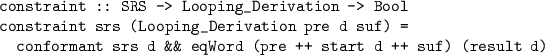
  This is the top-level constraint. The rewrite system srs is given at run-time. The derivation is unknown. An allocator represents a set of derivations with given maximal length (number of steps) and width (length of words).

Overall, the complete CO4 code consists of roughly 100 lines of code. The code snippets above indicate that the constraint system literally follows the textbook definitions. E.g., note the list-append (${+\!\!\!+}$) operators in constraint.

In contrast, Tyrolean Termination Tool 2 (TTT2, version 1.13)³ contains a hand-written propositional encoding for (roughly) the same constraint⁴ consisting of roughly 300 lines of (non-boilerplate) code. The TTT2 implementation explicitly allocates propositional variables (this is implicit in CO4), and explicitly manipulates indices (again, this is implicit in our ${+\!\!\!+}$).

Table 1 compares the performance of our implementation to that of TTT2 on some string rewriting systems of the Termination Problems Data Base⁵ collection. We restrict the search space in both tools to derivations of length 16 and words of length 16. All test were run on a Intel Xeon CPU with 3 GHz and 12 GB RAM. CO4’s test results can be replicated by running cabal test --test-options="loop-srs".

Table 1. Finding looping derivations in rewrite systems.

We note that CO4 generates larger formulas, for which, in general, MiniSat-2.2.0 needs more time to solve. There are rare cases where CO4’s formula is solved faster.

7 A Comparison to Curry

We compare the CO4 language and implementation to that of the functional logic programming language Curry [Han13], and its PAKCS-1.11.1 implementation (using the SICSTUS-4.2.3 Prolog system).

A common theme is that both languages are based on Haskell (syntax and typing), and extend this by some form of non-determinism, so the implementation has to realize some form of search.

In Curry, nondeterminism is created lazily (while searching for a solution). In CO4, nondeterminism is represented by additional Boolean decision variables that are created beforehand (in compilation).

The connection from CO4 to Curry is easy: a CO4 constraint program with top-level constraint $\mathtt {main\,\,{::}\,\, Known\,\, -> Unknown\,\, -> Bool}$ is equivalent to a Curry program (query) $\mathtt {main~k~u =:= True~where~u~free}$ (Fig. 2).

Fig. 2.

Two approaches to solve the $n$ queens problem

In the other direction, it is not possible to translate a Curry program to a CO4 program since it may contain locally free variables, a concept that is not supported in CO4. All free variables are globally defined by the allocator of the unknown parameter of the top-level constraint. For doing the comparison, we restrict to CO4 programs.

Example 6

We give an example where the CO4 strategy seems superior: the $n$ queens problem.

We compare our approach to a Curry formulation (taken from the PAKCS online examples collection) that uses the CLPFD library for finite-domain constraint programming. Our CO4 formulation uses built-in 8-bit binary numbers (Sect. 5) but otherwise is a direct translation. Note that with 8 bit numbers we can handle board sizes up to $2^7$: we add co-ordinates when checking for diagonal attacks.

Table 2 shows the run-times on several instances of the $n$ queens problem. CO4’s runtime is the runtime of the abstract program in addition to the runtime of the SAT-solver. The run-times for PAKCS were measured using the :set +time flag after compiling the Curry program in the PAKCS evaluator. Tests were done on a Intel Core 2 Duo CPU with 2.20 GHz and 4 GB RAM.

The PAKCS software also includes an implementation of the $n$ queens problem that does not use the CLPFD library. As this implementation already needs 6 seconds to solve a $n=8$ instance, we omit it in the previous comparison.

Table 2. Time for finding one solution of the $n$ queens problem

8 Discussion

In this paper we described the CO4 constraint language and compiler that allows to write constraints on tree-shaped data in a natural way, and to solve them via propositional encoding.

We presented the basic ideas for encoding data and translating programs, and gave an outline of a correctness proof for our implementation.

We gave an example where CO4 is used to solve an application problem from the area of termination analysis. This example shows that SAT compilation has advantages w.r.t. manual encodings.

We also gave an experimental comparison between CO4 and Curry, showing that propositional encoding is an interesting option for solving finite domain (FD) constraint problems. Curry provides lazy nondeterminism (creating choice points on-the-fly). CO4 does not provide this, since choice points are allocated before abstract evaluation.

Work on CO4 is ongoing. Our immediate goals are, on the one hand, to reduce the size of the formulas that are built during abstract evaluation, and on the other hand, to extend the source language with more Haskell features.

References

Baader, F., Nipkow, T.: Term Rewriting and all That. Cambridge University Press, New York (1998)
Bau, A., Waldmann, J.: Propositional encoding of constraints over tree-shaped data. CoRR, abs/1305.4957 (2013)
Codish, M., Giesl, J., Schneider-Kamp, P., Thiemann, R.: Sat solving for termination proofs with recursive path orders and dependency pairs. J. Autom. Reasoning 49(1), 53–93 (2012)
Davis, M., Logemann, G., Loveland, D.W.: A machine program for theorem-proving. Commun. ACM 5(7), 394–397 (1962)
Eén, N., Sörensson, N.: An extensible SAT-solver. In: Giunchiglia, E., Tacchella, A. (eds.) SAT 2003. LNCS, vol. 2919, pp. 502–518. Springer, Heidelberg (2004)
Hanus, M.: Functional logic programming: from theory to curry. In: Voronkov, A., Weidenbach, C. (eds.) Programming Logics. LNCS, vol. 7797, pp. 123–168. Springer, Heidelberg (2013)
Peyton Jones, S. (ed.): Haskell 98 Language and Libraries, The Revised Report. Cambridge University Press, Cambridge (2003)
Kurihara, M., Kondo, H.: Efficient BDD encodings for partial order constraints with application to expert systems in software verification. In: Orchard, B., Yang, C., Ali, M. (eds.) IEA/AIE 2004. LNCS (LNAI), vol. 3029, pp. 827–837. Springer, Heidelberg (2004)
Marques Silva, J.P., Sakallah, K.A.: Grasp - a new search algorithm for satisfiability. In: ICCAD, pp. 220–227 (1996)
Tseitin, G.S.: On the complexity of derivation in propositional calculus. In: Siekmann, J., Wrightson, G. (eds.) Automation of Reasoning. Symbolic Computation, pp. 466–483. Springer, Heidelberg (1983)
Zankl, H., Sternagel, C., Hofbauer, D., Middeldorp, A.: Finding and certifying loops. In: van Leeuwen, J., Muscholl, A., Peleg, D., Pokorný, J., Rumpe, B. (eds.) SOFSEM 2010. LNCS, vol. 5901, pp. 755–766. Springer, Heidelberg (2010)
Author information
Authors and Affiliations
Corresponding author
Editor information
Editors and Affiliations
Rights and permissions
Copyright information
© 2014 Springer International Publishing Switzerland
About this paper
Cite this paper
Bau, A., Waldmann, J. (2014). Propositional Encoding of Constraints over Tree-Shaped Data. In: Hanus, M., Rocha, R. (eds) Declarative Programming and Knowledge Management. INAP WLP WFLP 2013 2013 2013. Lecture Notes in Computer Science(), vol 8439. Springer, Cham. https://doi.org/10.1007/978-3-319-08909-6_3
Download citation
DOI: https://doi.org/10.1007/978-3-319-08909-6_3
Published:
Publisher Name: Springer, Cham
Print ISBN: 978-3-319-08908-9
Online ISBN: 978-3-319-08909-6
eBook Packages: Computer ScienceComputer Science (R0)