The Weak (2, 2)-Labelling Problem for Graphs with Forbidden Induced Structures

Abstract

The Weak (2, 2)-Conjecture is a graph labelling problem asking whether all connected graphs of at least three vertices can have their edges assigned red labels 1 and 2 and blue labels 1 and 2 so that any two adjacent vertices are distinguished either by their sums of incident red labels, or by their sums of incident blue labels. This problem emerged in a recent work aiming at proposing a general framework encapsulating several distinguishing labelling problems and notions, such as the well-known 1-2-3 Conjecture and so-called locally irregular decompositions.

In this work, we prove that the Weak (2, 2)-Conjecture holds for two classes of graphs defined in terms of forbidden induced structures, namely claw-free graphs and graphs with no pair of independent edges. One main point of interest for focusing on such classes of graphs is that the 1-2-3 Conjecture is not known to hold for them. Also, these two classes of graphs have unbounded chromatic number, while the 1-2-3 Conjecture is mostly understood for classes with bounded and low chromatic number.

1 Introduction

This work deals with several distinguishing labelling problems, taking part to a wide and vast area of research, as reported in several dedicated surveys on the topic, such as e.g. [7, 10]. More particularly, we focus on a subset of these problems revolving around the so-called 1-2-3 Conjecture, which can all be defined through the following unified terminology, introduced recently in [3].

Let G be a graph, and $\alpha ,\beta \ge 1$ be two positive integers. An $(\alpha ,\beta )$-labelling of G is an assignment $\ell$ of labels from $\{1,\dots ,\alpha \} \times \{1,\dots ,\beta \}$ to the edges of G, where each edge e gets assigned a label $\ell (e)=(x,y)$ with colour $x \in \{1,\dots ,\alpha \}$ and value $y \in \{1,\dots ,\beta \}$. Now, for every vertex v of G and any $i \in \{1,\dots ,\alpha \}$, we denote by $\sigma _i(v)$ the sum of the values of the labels with colour i assigned to the edges incident to v, which we call the i-sum of v. We say that $\ell$ is distinguishing if for every two adjacent vertices u and v of G, there is an $i \in \{1,\dots ,\alpha \}$ such that the i-sums of u and v differ, that is, if $\sigma _i(u) \ne \sigma _i(v)$.

Regarding these notions, it can be noted that if G is $K_2$, the complete graph of order 2, then there are no $\alpha ,\beta \ge 1$ such that G admits distinguishing $(\alpha ,\beta )$-labellings. Apart from this peculiar case, it is not too complicated to prove that, for any fixed $\alpha \ge 1$, there is a $\beta \ge 1$ such that distinguishing $(\alpha ,\beta )$-labellings of any graph G exist. For these reasons, in the context of distinguishing labellings, we generally focus on nice graphs, which are those graphs with no (connected) component isomorphic to $K_2$. Therefore, throughout this work, every graph we consider is thus implicitly assumed nice.

Fig. 1.

The current knowledge we have on whether all graphs admit distinguishing $(\alpha ,\beta )$-labellings, for fixed $\alpha ,\beta \ge 1$. For a pair $(\alpha ,\beta )$, the associated box is green if all graphs were proved to admit the corresponding labellings, the box is red if it is known that not all graphs admit the corresponding labellings, while the box is blue if the status is unknown. Arrows indicate existential implications. (Color figure online)

A natural question, now, is whether, for some fixed $\alpha ,\beta \ge 1$, every graph admits distinguishing $(\alpha ,\beta )$-labellings. It turns out, as mentioned earlier, that the literature actually provides answers for several values of $\alpha$ and $\beta$ (see Fig. 1).

• Note that if $\alpha ,\beta$ and $\alpha ',\beta '$ are such that $\alpha ' \ge \alpha$, $\beta ' \ge \beta$, and $(\alpha ,\beta ) \ne (\alpha ',\beta ')$, then any distinguishing $(\alpha ,\beta )$-labelling is a distinguishing $(\alpha ',\beta ')$-labelling.

• Distinguishing $(1,\beta )$-labellings are labellings where all labels are of the same colour, and all adjacent vertices should be distinguished according to their sums of incident labels. Such labellings are exactly those behind the so-called 1-2-3 Conjecture [9] of Karoński, Łuczak, and Thomason, which asks whether all graphs admit distinguishing (1, 3)-labellings. To date, the best result towards this is that they all admit distinguishing (1, 5)-labellings [8].

• Distinguishing $(\alpha ,1)$-labellings can be seen as edge-colourings where, for every two adjacent vertices, there must be a colour that is not assigned the same number of times to their incident edges. These labellings are those of the multiset version of the 1-2-3 Conjecture [1], which asks whether graphs admit distinguishing (3, 1)-labellings. This conjecture was proved in [11].

• In [3], the authors noticed that, given a distinguishing (1, 5)-labelling of some graph, by modifying the label colours and values in a particular way, we can derive a distinguishing (2, 3)-labelling of the same graph. Similarly, we can derive a distinguishing (3, 2)-labelling from a distinguishing (1, 5)-labelling.

• It is not too complicated to see that, in regular graphs, distinguishing (1, 2)-labellings and distinguishing (2, 1)-labellings are equivalent notions. In [2], it was proved that determining whether a cubic graph admits a distinguishing (1, 2)-labelling is NP-hard. Thus, there are infinitely many graphs that admit neither distinguishing (1, 2)-labellings nor distinguishing (2, 1)-labellings.

• Graphs admitting distinguishing (1, 1)-labellings are precisely the so-called locally irregular graphs, which are those graphs with no two adjacent vertices having the same degree. These graphs have been appearing frequently in the field, and have even been receiving dedicated attention, see e.g. [4].

From this all, there are thus only three pairs $(\alpha ,\beta )$ for which we are still not sure whether all graphs admit distinguishing $(\alpha ,\beta )$-labellings: (1, 3), which corresponds to the original 1-2-3 Conjecture; (1, 4), which is weaker than the 1-2-3 Conjecture since more label values are available (while, similarly, all labels are of the same colour); and (2, 2), which is the only pair for which we have two label colours to deal with. The latter pair leads to the following conjecture [3].

Weak (2, 2)-Conjecture. Every graph admits a distinguishing (2, 2)-labelling.

At first glance, the 1-2-3 Conjecture and the Weak (2, 2)-Conjecture might seem a bit distant. It is worth emphasising, however, that the former conjecture, if true, would imply the latter [5]. For this reason, the Weak (2, 2)-Conjecture can be perceived as a weaker version of the 1-2-3 Conjecture. Also, to get progress towards these conjectures, one can thus investigate the Weak (2, 2)-Conjecture for classes of graphs for which the 1-2-3 Conjecture is not known to hold. To date, the 1-2-3 Conjecture was mainly proved for 3-colourable graphs [10]. The weaker conjecture was mainly proved for 4-colourable graphs [5].

Theorem 1

([5]). The Weak (2, 2)-Conjecture holds for 4-colourable graphs.

Both conjectures were also proved for other classes of graphs, but not as significant. One reason why the chromatic number parameter appears naturally in this context is that having a proper vertex-colouring $\phi$ in hand can be helpful to design a distinguishing labelling, since $\phi$ informs on sets of vertices that are not required to be distinguished. One downside, however, is that making a labelling match $\phi$ somehow, might require lots of labels if $\phi$ itself contains lots of parts.

Here, we prove the Weak (2, 2)-Conjecture for two classes of graphs for which the 1-2-3 Conjecture (and thus the Weak (2, 2)-Conjecture, recall [5]) has not been proved. Besides, these classes have unbounded chromatic number, which, recall, is significant. Precisely, we prove the Weak (2, 2)-Conjecture for $K_{1,3}$-free graphs (with no induced claw) and $2K_2$-free graphs (with no pair of independent edges). Each result is proved by first dealing with the 5-colourable graphs of the class, before focusing on those with chromatic number at least 6.

Due to space limitation, in what follows we only present our result for $2K_2$-free graphs, its proof being a lighter, less technical version of that for $K_{1,3}$-free graphs, which require more involved arguments. We start in Sect. 2 with some preliminaries, before proving the Weak (2, 2)-Conjecture for $2K_2$-free graphs in Sect. 3. In concluding Sect. 4, we explain how to go from $2K_2$-free graphs to $K_{1,3}$-free graphs, summarising the arguments from our full-length paper [6].

2 Preliminaries

Let G be a graph, and $\ell$ be an $(\alpha ,\beta )$-labelling of G. If $\alpha =1$, then we will sometimes call $\ell$ a $\beta$-labelling for simplicity. Also, in such cases, instead of denoting the 1-sum of a vertex v by $\sigma _1(v)$, we will simply denote it as $\sigma (v)$, or as $\sigma _\ell (v)$ in case we want to emphasise that we refer to the labels assigned by $\ell$. Now, when considering the Weak (2, 2)-Conjecture and, thus, $(\alpha ,\beta )=(2,2)$, it will be more convenient to see the labels with colour 1 as red labels, and similarly those with colour 2 as blue labels. We will thus refer, for any vertex v, to the red sum $\sigma _\textrm{r}(v)$ of v (being $\sigma _1(v)$), and to the blue sum $\sigma _\textrm{b}(v)$ of v (being $\sigma _2(v)$).

We now point out a situation where, assuming a partial labelling of a graph is given, we can extend it to some edges so that some properties are preserved.

Lemma 1

Let G be a graph, H be a connected bipartite subgraph of G, and $\ell$ be a partial 2-labelling of G such that only the edges of H are not labelled. For any vertex w of H, there is a 2-labelling $\ell '$ of H such that, for every two adjacent vertices u and v of H with , we have

$$\sigma _\ell (u)+\sigma _{\ell '}(u) \ne \sigma _\ell (v)+\sigma _{\ell '}(v).$$

Proof

Let (U, V) denote the bipartition of H. We produce a 2-labelling $\ell '$ such that, for every vertex $u \ne w$ of H, we have $\sigma _\ell (u)+\sigma _{\ell '}(u) \equiv 0 \bmod 2$ if $u \in U$, and $\sigma _\ell (u)+\sigma _{\ell '}(u) \equiv 1 \bmod 2$ otherwise. This implies what we want to prove.

Start from all edges of H being assigned label 2 by $\ell '$. Now, consider any vertex u of H for which $\sigma _\ell (u)+\sigma _{\ell '}(u)$ does not satisfy the required condition above. Since H is connected, there is a path P from u to w that uses edges of H only. Now turn all 1’s assigned by $\ell '$ to the edges of P into 2’s, and conversely turn all 2’s into 1’s. As a result, note that $\sigma _\ell (v)+\sigma _{\ell '}(v)$ is not altered for every vertex v of H with , while both $\sigma _\ell (u)+\sigma _{\ell '}(u)$ and $\sigma _\ell (w)+\sigma _{\ell '}(w)$ had their parity altered. So $\sigma _\ell (u)+\sigma _{\ell '}(u)$ now verifies the desired condition.

Repeating those arguments until all vertices $u \ne w$ of H have $\sigma _\ell (u)+\sigma _{\ell '}(u)$ verifying the desired condition, we end up with $\ell '$ being as desired.   $\square$

We also recall a nice tool that proved to be very useful towards proving the multiset version of the 1-2-3 Conjecture from [1]. Let G be a graph. A balanced tripartition of G is a partition $V_0,V_1,V_2$ of V(G) fulfilling, for every vertex $v \in V_i$ with $i \in \{0,1,2\}$, that $d_{V_{i+1}}(v) \ge \max \{1,d_{V_i}(v)\}$ (all operations over the subscripts are modulo 3). That is, v has at least one neighbour in the next part $V_{i+1}$, and it actually has more neighbours in $V_{i+1}$ than in $V_i$. It turns out that graphs with large chromatic number admit such balanced tripartitions.

Theorem 2

([1]). Every graph G with $\chi (G)>3$ admits a balanced tripartition.

3 Graphs with No Induced Pair of Independent Edges

As mentioned earlier, we prove the Weak (2, 2)-Conjecture for $2K_2$-free graphs by treating the 5-chromatic ones first, and then those with large chromatic number.

Fig. 2.

Terminology used in the proof of Theorem 3, and the red sums and blue sums we aim at getting for the vertices by the designed (2, 2)-labelling. In the depicted situation, it is assumed that an upward edge of R is assigned red label 1

Theorem 3

Every $2K_2$-free graph with chromatic number 5 admits a distinguishing (2, 2)-labelling.

Proof

Let G be a $2K_2$-free graph with chromatic number 5. We construct a distinguishing (2, 2)-labelling of G assigning red labels 1 and 2 and blue labels 1 and 2. We can assume G is connected, since its 5-chromatic components can be handled through what follows, while Theorem 1 applies for its 4-colourable ones.

Let D be a maximal independent set of G, and set $\mathcal {R}=G-D$. Note that every vertex v in $\mathcal {R}$ is incident to at least one upward edge vu, i.e., going to D (so, $u \in D$). We say that a component of $\mathcal {R}$ is empty if it contains no edges, while it is non-empty otherwise. Since G is $2K_2$-free, note that $\mathcal {R}$ contains at most one non-empty component. Actually, $\mathcal {R}$ must contain exactly one non-empty component R as otherwise G would be bipartite, contradicting that its chromatic number is 5. Let now I denote the vertices from the empty components of $\mathcal {R}$, and let $\mathcal {H}$ be the subgraph of G induced by the edges incident to the vertices of I. Then $\mathcal {H}$ is bipartite, and because G is $2K_2$-free, $\mathcal {H}$ consists of only one component.

Since G is 5-chromatic, note that R is 4-chromatic; let thus $V_{0,0},V_{0,1},V_{1,0},V_{1,1}$ be parts forming a proper 4-vertex-colouring $\phi$ of R. We modify $\phi$, if needed, so that if v is a vertex of R with $d_R(v)=1$, then v belongs to $V_{0,0}$ or $V_{0,1}$ (note that this is clearly possible, since v has exactly one neighbour in R). Now order the vertices $v_1,\dots ,v_n$ in any way satisfying that, for every $i \in \{1,\dots ,n-1\}$, vertex $v_i$ is incident to at least one forward edge $v_iv_j$ (i.e., with $j>i$, which is a backward edge from $v_j$’s point of view). Such an ordering can be obtained e.g. by reversing the ordering in which vertices are encountered while performing a breadth-first search algorithm from any vertex (standing as the last vertex $v_n$).

We are now ready to start labelling the edges of G. We begin with all edges incident to the vertices of R. We consider the $v_i$’s one by one, following the ordering above, and for every vertex $v_i$ considered in that course, we assign a label to all upward edges (assigning them blue labels, except in one peculiar case) and forward edges (assigning them red labels only) incident to $v_i$ so that some desired red sum and blue sum are realised at $v_i$. When proceeding that way, note that, whenever considering a new vertex as $v_i$, only its backward edges can be assumed to be labelled, with red labels. The procedure goes as follows:

• If $i \ne n$, then $v_i$ is incident to forward edges. We start by assigning blue label 2 to all upward edges incident to $v_i$, and red label 2 to all forward edges incident to $v_i$. Assume $v_i \in V_{\alpha ,\beta }$. If , then we change to blue label 1 the label assigned to any one upward edge incident to $v_i$. Likewise, if , then we change to red label 1 the label assigned to any one forward edge incident to $v_i$. This way, we get $\sigma _\textrm{r}(v_i) \equiv \alpha \bmod 2$ and $\sigma _\textrm{b}(v_i) \equiv \beta \bmod 2$. In particular, by how we modified $\phi$ earlier, note that we must have $\sigma _\textrm{r}(v_i) \ge 2$ (either $d_R(v_i) \ge 2$ in which case this condition clearly holds; or $d_R(v_i) = 1$, in which case $\alpha =0$ and thus the only inner edge incident to $v_i$ is assigned red label 2, implying the condition).

• If $i=n$, then the only edges incident to $v_n$ that remain to be labelled are upward edges. Recall, in particular, that all backward edges incident to $v_n$ are assigned red labels. We consider two cases, assuming $v_n \in V_{\alpha ,\beta }$:

  • If $\sigma _\textrm{r}(v_n) \equiv \alpha \bmod 2$, then we assign blue labels to all upward edges incident to $v_n$, their values being chosen so that $\sigma _\textrm{b}(v_n) \equiv \beta \bmod 2$. In that case, we thus have $\sigma _\textrm{r}(v_n) \equiv \alpha \bmod 2$ and $\sigma _\textrm{b}(v_n) \equiv \beta \bmod 2$. Again, by how $\phi$ was modified earlier, we must have $\sigma _\textrm{r}(v_n) \ge 2$.

  • If , then we assign red label 1 to any one upward edge incident to $v_n$, while we assign blue labels to the other upward edges (if any) so that $\sigma _\textrm{b}(v_n) \equiv \beta \bmod 2$. Here, either $\sigma _\textrm{b}(v_n) \ne 0$ in which case $\sigma _\textrm{r}(v_n) \equiv \alpha \bmod 2$ and $\sigma _\textrm{b}(v_n) \equiv \beta \bmod 2$; or $\sigma _\textrm{b}(v_n)=0$ in which case all edges incident to $v_n$ are assigned red labels (implying that $\sigma _\textrm{r}(v_n) \ge 2$).

Note that, in all cases above, for all vertices $v_i \in V_{\alpha ,\beta }$, we guarantee $2 \le \sigma _\textrm{r}(v_i) \equiv \alpha \bmod 2$. Also, except maybe for $v_n$, we also guarantee $0 < \sigma _\textrm{b}(v_i) \equiv \beta \bmod 2$. Regarding $v_n$, either $\sigma _\textrm{b}(v_n)=0$, in which case $v_n$ is distinguished from all its neighbours in R through its blue sum, or $0<\sigma _\textrm{b}(v_n) \equiv \beta \bmod 2$, in which case $v_n$ is distinguished from its neighbours in R through its red sum and/or blue sum. Regarding the vertices of D, only one of them can be incident to an edge being assigned a red label, 1. So, for every $u \in D$, we have $\sigma _\textrm{r}(u) \le 1$, while $\sigma _\textrm{r}(v) \ge 2$ for every $v \in R$. Thus, currently, vertices of R are distinguished from their neighbours in D. If $\mathcal {H}$ has no edges, then all edges of G are labelled, and we have a distinguishing (2, 2)-labelling. So, below, we can assume $\mathcal {H}$ has edges.

We are now left with labelling the edges of $\mathcal {H}$, which, recall, consists of exactly one component. We consider two main cases:

• Assume there is some vertex $w \in \mathcal {H}$ with $\sigma _\textrm{r}(w) = 1$ (Fig. 2). Recall that there can be only one such vertex, which belongs to D and must be a neighbour of $v_n$. Recall also that the vertices of $D \cap V(\mathcal {H})$ can be incident to edges being currently assigned blue labels (being upward edges incident to vertices of R). Taking these labels into account, by Lemma 1 we can assign blue labels 1 and 2 to the edges of $\mathcal {H}$ so that any two of its adjacent vertices u and v with are distinguished by their blue sums. Since we did not modify labels assigned to edges incident to the vertices in R, and the edges of $\mathcal {H}$ are assigned blue labels only, the vertices of R remain distinguished from their neighbours due to arguments above. Regarding adjacent vertices of $\mathcal {H}$, they are either distinguished by their blue sums (if w is not involved), or because one of them has red sum 1 (if w is involved). So, here as well, we do not have conflicts.

• Assume no vertex of $\mathcal {H}$ currently has red sum at least 1. In this case, let w be any vertex of I. By Lemma 1, we can assign blue labels 1 and 2 to the edges of $\mathcal {H}$ so that, taking into account the other edges of G that are currently already assigned blue labels, and omitting w, any two adjacent vertices of $\mathcal {H}$ are distinguished by their blue sums. In case w has $d \ge 2$ neighbours $x_1,\dots ,x_d$ (which lie in D), then we further modify the labelling by changing to red label 1 the label assigned to $wx_1,\dots ,wx_d$. Again, we did not modify the red sums and blue sums of the vertices in R. Also, the only vertex of $D \cup I$ that might have red sum at least 2 is w (note that the $x_i$’s, if they exist, have red sum 1), which lies in I, the set of isolated vertices of $\mathcal {R}$ and thus cannot be adjacent to the vertices of R. Since the vertices of R have red sum at least 2, they thus cannot be involved in conflicts. Now, if $d_G(w)=1$, then, because G is not just an edge, the unique neighbour of w must have degree at least 2, meaning that w is necessarily distinguished from its unique neighbour. Otherwise, i.e., w has $d \ge 2$ neighbours $x_1,\dots ,x_d \in D$, then $\sigma _\textrm{r}(w) = d \ge 2$ while the $x_i$’s have red sum 1, and thus w cannot be involved in conflicts. Regarding the $x_i$’s, they have red sum 1, so they cannot be in conflict with their neighbours of $\mathcal {H}$ different from w, since they have red sum 0. Finally, for every vertex of $\mathcal {H}$ not in $\{w,x_1,\dots ,x_d\}$, note that we did not modify its blue sum when introducing red labels. So we still have that any two such adjacent vertices are distinguished by their blue sums, by how we applied Lemma 1. So, no conflicts exist in G.

The resulting (2, 2)-labelling of G is thus distinguishing, as desired.    $\square$

Fig. 3.

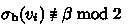
Terminology used in the proof of Theorem 4, and the red sums and blue sums we aim at getting for the vertices by the designed (2, 2)-labelling.

Theorem 4

Every $2K_2$-free graph with chromatic number at least 6 admits a distinguishing (2, 2)-labelling.

Proof

Let G be a $2K_2$-free graph with chromatic number at least 6. We construct a distinguishing labelling of G assigning red labels 1 and 2 and blue labels 1 and 2. Again, we may assume that G is connected.

Let $D_1$ be a maximal independent set of G. Note that every vertex of $G-D_1$ has at least one neighbour in $D_1$. Now let $D_2$ be a maximal independent set of $G-D_1$. Similarly, every vertex of $G-D_1-D_2$ has at least one neighbour in $D_2$. Since $\chi (G) \ge 6$, note that $\chi (G-D_1-D_2) \ge 4$. According to Theorem 2, there is thus a balanced tripartition $V_0, V_1, V_2$ of $G-D_1-D_2$ (see Fig. 3). Note that $D_1$, $D_2$, $V_0$, $V_1$, and $V_2$ form a partition of V(G). An upward edge of G is an edge with one end in $V_0 \cup V_1 \cup V_2$ and the other in $D_1 \cup V_2$. An inner edge of G is an edge with both ends in some $V_i$. If $u \in V_i$ and $u' \in V_{i+1}$ (where the operations over the subscripts of the $V_i$’s are modulo 3) are adjacent for some $i \in \{0,1,2\}$, then $uu'$ is a forward edge from u’s perspective, and a backward edge from that of $u'$. Because G is $2K_2$-free, note that all three of $G[V_0]$, $G[V_1]$, and $G[V_2]$ contain at most one component with edges each.

We denote by $\mathcal {H}$ the set of the components of $G[D_1 \cup D_2]$. Since every vertex of $D_2$ has neighbours in $D_1$, note that $\mathcal {H}$ has edges. Since G is $2K_2$-free, there is exactly one component H of $\mathcal {H}$ that is non-empty, i.e., contains edges. $\mathcal {H}$ can also contain empty components, which consist in a single vertex of $D_1$.

We design the desired (2, 2)-labelling of G following four steps. First, we label all inner, upward, and forward edges incident to the vertices of $V_0$ so that they fulfil certain properties on $\sigma _\textrm{r}$ and $\sigma _\textrm{b}$. Second and third, we then achieve the same for the vertices of $V_1$ and $V_2$. Last, we label the edges of $\mathcal {H}$.

Step 1: Labelling the inner, upward, and forward edges of $V_0$ .

We start by labelling the following edges of G:

• 1. We first assign blue label 2 to all inner edges incident to vertices of $V_0$.

• 2. We then consider every vertex u of $V_0$ in turn, assign red label 2 to all upward edges incident to u, and eventually change to red label 1 one of these red labels so that the red sum of u becomes odd.

• 3. We now distinguish two cases, through which we get to defining a special vertex $w \in D_2$ that will be useful later on, by the last step of the proof.

  • $|V_0|=1$, i.e., $G[V_0]$ is a single vertex u. Here, we assign blue label 2 to all forward edges incident to u. We also modify the labelling further as follows. Set w as any neighbour of u in $D_2$. Note that, by swapping the red labels assigned to uw and another upward edge incident to u, we can, if necessary, assume uw is assigned red label 2. We then change the label assigned to uw to blue label 1.

  • Otherwise, i.e. $|V_0| \ge 2$. Here, let $u_1,\dots ,u_n$ be an arbitrary ordering over the vertices of $V_0$, and consider the $u_i$’s one by one in order. Since extra modifications must be made around $u_1$, let us consider that vertex specifically before describing the general case. Just as in the previous case, let w be any neighbour of $u_1$ in $D_2$. Again, we can swap labels assigned to upward edges, if necessary, so that $u_1w$ is assigned red label 2. Then we change the label assigned to $u_1w$ to blue label 1, before assigning blue label 2 to all forward edges incident to $u_1$. Now, for every subsequent $u_i$ with $i \ge 2$, denote by $u_{i_1},\dots ,u_{i_d}$ the $d \ge 0$ neighbours of $u_i$ in $V_0$ that precede $u_i$ in the ordering. If $d=0$, then assign blue label 2 to all forward edges incident to $u_i$. Now, if $d \ge 1$, then recall that $u_i$ is incident to $d_{V_1}(u_i) \ge d$ forward edges. By assigning red label 2 to none, one, two, etc., or all of these edges, and blue label 2 to all others, we can increase the red sum of $u_i$ by any amount in $\{0,2,\dots ,2d_{V_1}(u_i)\}$, which set contains $d_{V_1}(u_i)+1 \ge d+1$ elements. There is thus a way to assign red label 2 to at most d forward edges incident to $u_i$, and blue label 2 to the rest, so that the red sum of $u_i$ is different from the red sums of $u_{i_1},\dots ,u_{i_d}$.

Once the steps above have been performed fully, note that all inner, upward, and forward edges incident to the vertices of $V_0$ are assigned a label. Also, for every vertex $u \in V_0$, we currently have $\sigma _\textrm{r}(u) \equiv 1 \bmod 2$, and it can be checked that also $\sigma _\textrm{b}(u) \ge 2$. Furthermore, every two adjacent vertices of $V_0$ currently have their red sums being different. Remark last that all upward edges incident to the vertices of $V_0$ are assigned red labels, except for exactly one edge incident to w, which is assigned blue label 1.

Step 2: Labelling the inner, upward, and forward edges of $V_1$ .

Due to the previous step, note also that all backward edges incident to the vertices in $V_1$ are labelled with red label 2 and blue label 2. So, one should keep in mind that, currently, $\sigma _\textrm{r}(u)$ is even for every $u \in V_1$.

We now label more edges as follows:

• 1. First, we assign blue label 2 to all inner edges incident to vertices of $V_1$.

• 2. Second, we consider every vertex u of $V_1$ in turn. Recall that u is incident to at least two upward edges. We assign red label 2 to all these edges. If necessary, we change the label assigned to two of these edges to red label 1, so that $\sigma _\textrm{r}(u) \equiv 2 \bmod 4$.

• 3. Third, let $u_1,\dots ,u_n$ be an arbitrary ordering over the vertices of $V_1$, and consider the $u_i$’s one by one in turn. For every $u_i$ considered that way, denote by $u_{i_1},\dots ,u_{i_d}$ the $d \ge 0$ neighbours of $u_i$ in $V_1$ that precede $u_i$ in the ordering. If $d=0$, then assign blue label 2 to all forward edges incident to $u_i$. Now, if $d \ge 1$, then recall that $u_i$ is incident to $d_{V_2}(u_i) \ge d$ forward edges. Thus, through assigning blue labels to these edges, we can make the blue sum of $u_i$ vary by any amount in the set $\{d_{V_2}(u_i),\dots ,2d_{V_2}(u_i)\}$, which contains $d_{V_2}(u_i)+1 \ge d+1$ elements. Thus, it is possible to assign blue labels to the forward edges incident to $u_i$ so that its resulting blue sum is different from that of $u_{i_1},\dots ,u_{i_d}$.

After completing the previous steps, all edges incident to the vertices in $V_1$ are labelled. For every vertex $u \in V_1$, we get $\sigma _\textrm{r}(u) \equiv 2 \bmod 4$, and also $\sigma _\textrm{b}(u) \ge 2$, because either $d_{V_1}(u)=0$ and at least one forward edge incident to u is assigned blue label 2, or $d_{V_1}(u)>0$ and at least one inner edge incident to u is assigned blue label 2. Also, adjacent vertices of $V_1$ are distinguished by their blue sums, and all upward edges incident to the vertices of $V_1$ are assigned red labels.

Step 3: Labelling the inner, upward, and forward edges of $V_2$ .

Note that after performing the previous step, all backward edges incident to the vertices of $V_2$ are assigned blue labels; so, their red sum is currently 0.

We now perform the following:

• 1. We assign blue label 2 to all inner edges incident to vertices in $V_2$.

• 2. We then consider every vertex u of $V_2$ in turn, which, recall, is incident to at least two upward edges. We assign red label 2 to all these edges before, if necessary, changing the label assigned to two of these edges to red label 1, so that $\sigma _\textrm{r}(u) \equiv 0 \bmod 4$.

• 3. We finish off this step similarly as the previous one. Let $u_1,\dots ,u_n$ be any ordering over the vertices of $V_2$, and consider the $u_i$’s one after the other. For every $u_i$, let $u_{i_1},\dots ,u_{i_d}$ be the $d \ge 0$ neighbours of $u_i$ in $V_2$ that precede $u_i$ in the ordering. If $d=0$, then assign blue label 2 to all forward edges incident to $u_i$. Otherwise, if $d \ge 1$, then recall that $u_i$ is incident to $d_{V_0}(u_i) \ge d$ forward edges. Via assigning blue labels to these edges, we can thus make the blue sum of $u_i$ increase by any value in $\{d_{V_0}(u_i),\dots ,2d_{V_0}(u_i)\}$, which set contains $d_{V_0}(u_i)+1 \ge d+1$ elements. Thus, we can assign blue labels to the forward edges incident to $u_i$ so that its blue sum is different from that of $u_{i_1},\dots ,u_{i_d}$.

Once this step achieves, all edges incident to vertices in $V_0 \cup V_1 \cup V_2$ are labelled. For every vertex $u \in V_2$, we have $\sigma _\textrm{r}(u) \equiv 0 \bmod 4$ and $\sigma _\textrm{b}(u) \ge 2$. Every two adjacent vertices of $V_2$ are distinguished by their blue sums, while all upward edges incident to the vertices in $V_2$ are assigned red labels. It is important to emphasise also that assigning blue labels to the edges joining vertices of $V_2$ and $V_0$ altered the blue sums of the vertices in $V_0$, which is not an issue since the adjacent vertices of $V_0$ are distinguished by their red sums, which were not altered. So, any two adjacent vertices in $V_0$ remain distinguished, and similarly for any two adjacent vertices in $V_1$. Finally, note that any two adjacent vertices in distinct $V_i$’s are distinguished by their red sums having different values modulo 4.

Step 4: Labelling the edges of $\mathcal {H}$ .

Recall that, at this point, we have $\sigma _\textrm{b}(v)=0$ for every vertex $v \in D_1 \cup D_2 \setminus \{w\}$ and $\sigma _\textrm{b}(w)=1$, while $\sigma _\textrm{b}(u) \ge 2$ for every vertex $u \in V_0 \cup V_1 \cup V_2$. In particular, if $v \in D_1$ belongs to an empty component of $\mathcal {H}$, then all edges incident to v are already labelled, and v is distinguished from its neighbours due to its blue sum.

Recall that H denotes the unique non-empty component of $\mathcal {H}$, and that H actually contains all edges of G that remain to be labelled. Recall also that H contains w, a special vertex we defined in the first labelling step, which is the only vertex of H having non-zero blue sum. According to Lemma 1, we can assign red labels 1 and 2 to the edges of H so that, even when taking into account the red labels assigned to the upward edges incident to the vertices in $V_0 \cup V_1 \cup V_2$, any two adjacent vertices of H different from w are distinguished by their red sums. Since $\sigma _\textrm{b}(w)=1$ while $\sigma _\textrm{b}(v)=0$ for every $v \in V(\mathcal {H}) \setminus \{w\}$, vertex w is also distinguished from its neighbours in $\mathcal {H}$. These conditions guarantee we have not introduced any conflicts involving vertices of $D_1 \cup D_2$ and vertices of $V_0 \cup V_1 \cup V_2$.

Thus, the resulting (2, 2)-labelling of G is distinguishing.    $\square$

4 From $2K_2$-free Graphs to $K_{1,3}$-free Graphs, and Beyond

As mentioned earlier, we also proved the Weak (2, 2)-Conjecture for claw-free graphs in the full paper [6], in a way that is quite reminiscent of how we proved Theorems 3 and 4. The structure of $2K_2$-free graphs being much more constrained than that of $K_{1,3}$-free graphs, this required involved refinements over our arguments; in particular:

• The main issue in order to adapt Theorem 3 to $K_{1,3}$-free graphs, is that $\mathcal {R}$ can now have several non-empty components, and similarly for $\mathcal {H}$. Then, by leading the proof the exact same way for every non-empty component of $\mathcal {R}$, multiple upward edges can now be assigned red label 1. Fortunately, the fact that G is claw-free implies that every $u \in D$ neighbours vertices from at most two components of $\mathcal {R}$, meaning that $\sigma _\textrm{r}(u) \le 2$. So there can be conflicts between vertices of $\mathcal {R}$ and D, but we can get rid of those by altering the labelling around very local structures of G.

• Regarding adapting Theorem 4 to $K_{1,3}$-free graphs, the main issue is that $\mathcal {H}$ can now have several non-empty components, the most troublesome of which can consist of a single edge $v_1v_2$ with $v_1 \in D_1$ and $v_2 \in D_2$. The problem is that distinguishing $v_1$ and $v_2$ has nothing to do with the label assigned to $v_1v_2$; in particular, $v_1$ and $v_2$ might get in conflict because of how we labelled the upward edges, when dealing with the vertices of $V_0 \cup V_1 \cup V_2$. We deal with this issue through being extra cautious when labelling upward edges, to make sure such situations do not occur. This requires us to also modify our sum rules by a bit. For instance, we allow vertices of $V_0$ to have a red sum that is not odd, provided their neighbourhood satisfies some conditions.

In both cases, the final step of labelling the edges of $\mathcal {H}$ is also slightly trickier, due to the fact that we have less control over the labels assigned to upward edges. Fortunately, when G is claw-free, $\mathcal {H}$ is actually a bipartite graph with maximum degree at most 2, a structure which is quite favourable, and which we manage to deal with using algebraic tools (such as the Combinatorial Nullstellensatz).

To go farther on this topic, it could be interesting to investigate the Weak (2, 2)-Conjecture for more classes of graphs defined in terms of forbidden structures, such as triangle-free graphs, or graphs with large girth in general. One could wonder also about graphs in which many short cycles are present, such as chordal graphs. Another class could be that of $P_4$-free graphs (cographs).

References

Addario-Berry, L., Aldred, R.E.L., Dalal, K., Reed, B.A.: Vertex colouring edge partitions. J. Comb. Theory. Ser. B 94(2), 237–244 (2005)
Ahadi, A., Dehghan, A., Sadeghi, M.-R.: Algorithmic complexity of proper labeling problems. Theor. Comput. Sci. 495, 25–36 (2013)
Baudon, O., et al.: A general decomposition theory for the 1-2-3 Conjecture and locally irregular decompositions. Discret. Math. Theor. Comput. Sci. 21(1), 2 (2019)
Baudon, O., Bensmail, J., Przybyło, J., Woźniak, M.: On decomposing regular graphs into locally irregular subgraphs. Eur. J. Comb. 49, 90–104 (2015)
Bensmail, J.: On a graph labelling conjecture involving coloured labels. Discuss. Math. Graph Theory (in press)
Bensmail, J., Hocquard, H., Marcille, P.-M.: The weak \((2,2)\)-Labelling Problem for graphs with forbidden induced structures. Preprint (2022). https://hal.archives-ouvertes.fr/hal-03784687
Gallian, J.A.: A dynamic survey of graph labeling. Electron. J. Comb. 1, DS6 (2021)
Kalkowski, M., Karoński, M., Pfender, F.: Vertex-coloring edge-weightings: towards the 1-2-3 conjecture. J. Comb. Theory. Ser. B 100, 347–349 (2010)
Karoński, M., Łuczak, T., Thomason, A.: Edge weights and vertex colours. J. Comb. Theory. Ser. B 91, 151–157 (2004)
B. Seamone. The 1–2-3 Conjecture and related problems: a survey. Preprint (2012). http://arxiv.org/abs/1211.5122
Vučković, B.: Multi-set neighbor distinguishing \(3\)-edge coloring. Discret. Math. 341, 820–824 (2018)
Author information
Authors and Affiliations
Corresponding author
Editor information
Editors and Affiliations
Rights and permissions
Copyright information
© 2023 The Author(s), under exclusive license to Springer Nature Switzerland AG
About this paper
Cite this paper
Bensmail, J., Hocquard, H., Marcille, PM. (2023). The Weak (2, 2)-Labelling Problem for Graphs with Forbidden Induced Structures. In: Bagchi, A., Muthu, R. (eds) Algorithms and Discrete Applied Mathematics. CALDAM 2023. Lecture Notes in Computer Science, vol 13947. Springer, Cham. https://doi.org/10.1007/978-3-031-25211-2_16
Download citation
DOI: https://doi.org/10.1007/978-3-031-25211-2_16
Published:
Publisher Name: Springer, Cham
Print ISBN: 978-3-031-25210-5
Online ISBN: 978-3-031-25211-2
eBook Packages: Computer ScienceComputer Science (R0)