Quantum Rewinding for Many-Round Protocols

Abstract

We investigate the security of succinct arguments against quantum adversaries. Our main result is a proof of knowledge-soundness in the post-quantum setting for a class of multi-round interactive protocols, including those based on the recursive folding technique of Bulletproofs. To prove this result, we devise a new quantum rewinding strategy, the first that allows for rewinding across many rounds. This technique applies to any protocol satisfying natural multi-round generalizations of special soundness and collapsing. For our main result, we show that recent Bulletproofs-like protocols based on lattices satisfy these properties, and are hence sound against quantum adversaries.

1 Introduction

Succinct arguments [13, 20] allow a prover to convince a verifier that a statement x belongs to a language $\mathcal {L}$, with communication shorter than the witness length for the corresponding relation. Succinct arguments have become a cornerstone of modern cryptography and fueled the development of many real-world applications, such as verifiable computation and anonymous cryptocurrencies. Recent years have seen an explosion of new constructions of succinct arguments, based on a variety of cryptographic assumptions.

However, the advent of quantum computation poses a significant threat to these advancements. On the one hand, Shor’s algorithm [22] forces us to transition to cryptographic systems based on post-quantum assumptions, such as the hardness of the learning with errors (LWE) problem [21]. On the other hand, some known techniques to prove security of cryptographic protocols no longer apply in the post-quantum regime, due to the fundamentally different nature of quantum information. Most notable are rewinding techniques, which are ubiquitous in security proofs for succinct arguments.

In a rewinding proof, it is argued that an adversary that succeeds on a single random challenge with high enough probability must succeed on multiple challenges. This classically intuitive idea fails in the quantum setting, because measuring the adversary’s response to one challenge causes an irreversible loss of information which may render it useless for answering other challenges.

An important family of succinct arguments are interactive protocols based on the recursive folding technique of [7, 10], also known in the literature as Bulletproofs. Leveraging algebraic properties of cryptographic schemes, Bulletproofs-like protocols can achieve much smaller proof sizes than PCP- and IOP-based succinct arguments [6, 13] while retaining the benefit of a public-coin setup. Unlike PCP- and IOP-based arguments, however, the original Bulletproofs constructions are not post-quantum secure, being based on the hardness of the discrete logarithm problem. This has motivated a line of work that aims to design “post-quantum Bulletproofs” [2, 4, 8, 9]. While these works do not rely on cryptographic assumptions which are quantum-insecure, their analysis of post-quantum security is only heuristic, in the sense that soundness is only shown against a classical adversary. Motivated by this state of affairs, we ask the following question:

Can we prove post-quantum security for Bulletproofs-like protocols?

Known techniques for rewinding quantum adversaries [11, 24] do not appear to generalize to multi-round challenge-response protocols, let alone to logarithmic-round protocols like Bulletproofs. Thus, answering the above question requires us to develop new quantum rewinding techniques.

1.1 Our Results

In this work, we show that a class of “recursive” many-round interactive protocols is knowledge-sound against quantum adversaries. As a special case, we establish that lattice-based Bulletproofs protocols are post-quantum secure, assuming the quantum hardness of LWE. Loosely speaking, our main result can be restated as follows.

Theorem 1

(Informal). Assuming the quantum hardness of the (Ring-)LWE problem, lattice-based Bulletproofs protocols are knowledge-sound against quantum algorithms.

Our main result is obtained by developing two technical contributions of independent interest:

• Fold-Collapsing Hash: We show that the lattice-based hash function $\textsf{Hash}_\textbf{A} (\textbf{x}) = \textbf{A} \textbf{x} \bmod q$, where $\textbf{A}$ is sampled uniformly at random and $\textbf{x}$ is a “short” vector, satisfies a strong collapsing property¹. Intuitively, we show that $\textsf{Hash}_\textbf{A}$ remains collapsing even when the key $\textbf{A}$ is compressed via linear combinations of its columns with coefficients being short units in the base ring. This fold-collapsing property can be based on a variety of computational assumptions, including the (Ring-)LWE assumption.

• Quantum Tree Rewinding: We develop a new quantum rewinding technique that allows us to extract from multi-round interactive protocols with certain collapsing and “recursive special soundness” properties. Our method combines the state-repair procedure of [11] with a probability estimation step that determines the success probability of the adversary on a given sub-tree. Combined with the collapsing property above and the recursive special soundness of Bulletproofs-like arguments, this establishes the post-quantum security of these protocols.

1.2 Related Work

The witness folding technique for constructing succinct arguments was first introduced by Bootle et al. [7] and later optimized by Bünz et al. [10], who called their protocols Bulletproofs. The term “Bulletproofs” is now used to refer to a family of succinct arguments with a certain recursive structure. The early Bulletproofs protocols [7, 10] prove quadratic relations of exponents of elements in prime-order cyclic groups, and their soundness relies on the discrete logarithm assumption over these groups. Lai, Malavolta, and Ronge [14] generalized the folding technique to prove quadratic relations over bilinear pairing groups under a variant of the discrete logarithm assumption defined over these groups. As the discrete logarithm problems can be solved by Shor’s algorithm [22] in quantum polynomial time, none of these protocols are post-quantum sound.

While it is necessary to consider non-linear relations to obtain an argument for NP, Attema and Cramer [3] showed how to linearize the non-linear relations using secret-sharing techniques, and apply the folding technique to compress the argument for the linearized relations. Although their protocols for proving linear relations over groups are in fact unconditionally sound, they are trivial in the quantum setting because the relations that they prove are in $\textsf{BQP}$.

Bootle et al. [9] adapted the Bulletproofs folding technique to the lattice setting, giving a succinct argument for proving knowledge of the witness of a short integer solution (SIS) instance, i.e. a short vector $\textbf{x}$ satisfying $\textbf{A} \textbf{x} = \textbf{y} \bmod q$, over the m-th cyclotomic ring with m being a power of 2. The protocol, however, has large “slack”: the knowledge extractor is only able to extract a short vector $\textbf{x}'$ satisfying $\textbf{A} \textbf{x}' = 8^t \cdot \textbf{y} \bmod q$, where $\ell = 2^t$ is the dimension of the witness $\textbf{x}$. Albrecht and Lai [2] revisited this protocol and reduced the slack from $8^t$ to $2^t$ with a careful choice of the challenge set R. They further eliminated the slack in the case of prime-power cyclotomic rings, i.e. when m is a power of a polynomially-large prime. Attema, Cramer, and Kohl [4] improved the soundness analysis of [2, 9], reducing the knowledge error from $O(\log \ell /|R|)$ to $2 \log \ell /|R|$, which is tight. Bootle, Chiesa, and Sotiraki [8] proposed the abstract framework of sumcheck arguments which captures all Bulletproofs-like protocols, particularly lattice-based ones, mentioned above. Although lattice-based Bulletproofs for proving SIS relations are shown to be unconditionally sound against classical provers, the security proofs implicitly assume that the success probability of a prover remains unchanged after rewinding, which is generally false in the quantum setting.

1.3 Organization

In Sect. 2 we give an overview of our technical results. In Sect. 3 we recall standard preliminaries. In Sect. 4 we recall the notion of public-coin interactive arguments and introduce the notions of recursive special soundness and last-round collapsing. In Sect. 5 we show that protocols satisfying these properties are also knowledge-sound, even against quantum provers. In Sect. 6 we study the collapsing properties of hash function families implicit in lattice-based Bulletproof protocols. In the full version we build upon the results of Sect. 6 to show that lattice-based Bulletproof protocols are recursive special sound and last-round collapsing, and hence knowledge-sound, even against quantum provers.

2 Technical Overview

We give a brief overview of the main technical steps of our work. Before delving into the details of our analysis, we summarize the main conceptual steps of our proof:

• Step I: We formalize a family of public-coin protocols $\varSigma$ that satisfy two main properties of interest, namely recursive special soundness and last-round collapsing.

• Step II: We describe a new quantum rewinding strategy that allows us to extract a witness from any recursive special sound and last-round collapsing protocol of the above defined family.

• Step III: We show that the lattice-based hash function $\textsf{Hash}_\textbf{A} (\textbf{x}) = \textbf{A} \textbf{x}$ is fold-collapsing, assuming that the (Ring-)LWE problem is intractable for quantum algorithms.

• Step IV: Using the result from the previous step, we show that lattice-based Bulletproofs protocols are recursive special sound and last-round collapsing.

The remainder of the technical overview will be split into two parts, detailing Step I–II and Step III–IV respectively.

2.1 Quantum Rewinding

We first establish some context. Consider a $(2t+1)$-message public-coin interactive argument $\varSigma$ where both the prover and the verifier input a statement x and the prover additionally inputs a witness w. The first 2t rounds of the protocol consists of the prover sending a “commitment” $z_i$ and the verifier sending a challenge $r_i$ for $i \in [t]$. The protocol ends with the prover sending a response $w_{t+1}$ and the verifier outputting a single bit. The protocol $\varSigma$ is k-tree-special sound, or $(k,\ldots ,k)$-special sound, for a relation $\mathfrak {R}$ if the following holds: There exists an efficient extractor $E$ which, given a statement x and complete k-ary tree of (edge-)depth t where the nodes and edges in each root-to-leaf path are labelled by a transcript $(z_1,r_1,\ldots ,z_t,r_t,w_{t+1})$ of $\varSigma$ which is accepting, extracts a witness w satisfying $\mathfrak {R} (x,w) = 1$.

In the following, we first review how tree-special soundness classically implies knowledge-soundness, and discuss where the classical reduction fails in the quantum setting. We then overview how post-quantum knowledge-soundness can be proven for protocols which satisfy a strengthening of tree special soundness along with a natural “collapsing” property.

Classical Tree Rewinding. To prove that a tree-special sound argument is knowledge-sound, the classical extraction proof (e.g. given in [9]) is based on the tree extraction technique of [7]. This technique obtains a k-ary tree of transcripts using a simple recursive strategy. This tree can then be provided to E in order to obtain the witness. For $i \in [t]$, [7] define subtree extractors $T_{i}$ which, given a transcript prefix, obtain a k-ary subtree rooted at that prefix:

$\underline{T_{i}(r_1,\ldots ,r_{i-1}):}$

• 1. Let $\tau$ be a graph containing a single (root) node v.

• 2. Query the adversary at $(r_1,\ldots ,r_{i-1})$ to obtain the i-th round commitment $z_{i}$. Label v with $z_i$.

• 3. Repeat until v has k children: Choose $r_{i} \leftarrow R_i$ uniformly at random, and run $\tau ' \leftarrow T_{i+1}(r_1,\ldots ,r_{i})$. If $T_{i+1}$ does not abort, attach $\tau '$ to v via an edge labelled with $r_{i}$. If $T_{i+1}$ aborts, and this is the first loop iteration, then abort.

• 4. Return $\tau$.

The base case $T_{t+1}(r_1,\ldots ,r_{t})$ queries the adversary at $(r_1,\ldots ,r_{t})$ to obtain a full protocol transcript $(z_1,\ldots ,z_{t+1})$ and returns $z_{t+1}$ if that transcript is accepting (and otherwise aborts). The italicized condition above ensures that the procedure runs in expected polynomial time. Concretely, let $\varepsilon$ denote the probability for $r_{i}$ chosen uniformly at random that $T_{i+1}(r_1,\ldots ,r_{i})$ does not abort. The number of calls that $T_{i}$ makes to $T_{i+1}$ is then 1 with probability $1 - \varepsilon$ (due to the italicized condition) and $1 + (k-1)/\varepsilon$ (in expectation) with probability $\varepsilon$. Hence the overall expected number of calls is k, and by induction $T_{i}$ runs in expected time $O(k^{t-i} \cdot t_{A})$, where $t_A$ is the running time of the adversary.

Quantum Tree Rewinding. Moving now to the quantum setting, the immediate problem is that Step 3 is a rewinding step: The above argument implicitly uses the fact that a classical adversary can be rewound to ensure that the success probability of $T_{i+1}$ in each iteration is always $\varepsilon$. For quantum adversaries, the situation is more complicated, since measurements are in general irreversible operations. Known techniques [11, 24] allow one to recover this type of rewinding in the quantum setting, provided the protocol satisfies a special “collapsing” condition.

Roughly speaking, this condition says the measurement performed by the reduction in the rewinding loop to obtain the response (in this case $\tau$) is indistinguishable (to the adversary) from a binary measurement of whether the obtained response is valid or not (in this case, whether $T_{i+1}$ aborts). Unfortunately, for the extractor above for general tree-special sound protocols we do not have this guarantee. The issue is that $\tau$ contains information about the set of challenges to which the adversary produces an accepting response. Measuring this information can cause the adversary’s state to be disturbed in a detectable way. As a result, we do not know how to achieve general tree extraction in the quantum setting.

Instead, we observe that Bulletproofs-like protocols satisfy additional structural properties such that extracting the full tree is not necessary. Specifically, we can identify a family of protocols $(\varSigma _i)_{i=0}^t$ associated to $\varSigma$, where $\varSigma _i$ has $2i+1$ messages, $\varSigma _t = \varSigma$ and $\varSigma _0$ is a noninteractive protocol where the prover sends w and the verifier checks $\mathfrak {R} (x,w)$.

This family has the property that, given a k-ary tree of accepting transcripts for $\varSigma _{i}$, we can obtain a k-ary tree of accepting transcripts for $\varSigma _{i-1}$ by applying only “local” operations at the i-th layer: specifically, we compute a new label for each node $v_i$ at depth i by applying a function $E_{i}$ to the labels of its children. With this structural property, we can modify $T_i$ (for all i) to directly output a witness (label) $w_i$ instead of a tree $\tau$. As a result, $T_0$ will directly output a witness w for x.

Moreover, we identify that if each $\varSigma _i$ satisfies another property called last-round collapsing and, crucially, $T_{i+1}$ is executed projectively by $T_{i}$, then measuring the output of $T_{i+1}$ is in fact indistinguishable from a binary measurement. It turns out that the key technical challenge here is the projectivity of $T_{i+1}$.

The Extractor. A general quantum measurement given by a circuit can be implemented projectively in a standard way using the principle of deferred measurement. Specifically, a circuit C has a corresponding unitary dilation U (given by replacing measurement gates with controlled-NOTs); the projective implementation is obtained by applying U, measuring the output register, and then applying $U^{\dagger }$.

Unfortunately, this method only applies to circuits, whereas in the above template, $T_{i+1}$ is an algorithm with variable (expected polynomial) runtime. The unitary dilation of an expected (quantum) polynomial time (EQPT) algorithm is not generally efficiently implementable². To avoid this problem, we design an extractor where the recursive call is to a strict polynomial-time algorithm. To give a sense of our construction, we will (for now) return to the classical setting. A natural first attempt is to simply truncate $T_{i+1}$ to some strict number of repetitions N; applying this to all layers of the tree yields an extractor that makes $N^t$ calls to the adversary. How large does N need to be? By Markov’s inequality, the error incurred by truncation is O(k/N); hence to achieve any guarantee, we require that $N = \varOmega (k/\varepsilon )$. As a result, $N^t$ is superpolynomial (since $\varepsilon$ is an arbitrary inverse polynomial).

The key to overcoming this issue is to ensure that, no matter how many repetitions of Step 3 we execute, we only make k recursive calls. In particular, we must guarantee that whenever we make a call to $T_{i+1}$, it succeeds with high probability. To do this in the classical setting, we can modify the extractor as follows.

$\underline{T_{i,\varepsilon }(r_1,\ldots ,r_{i-1}):}$

• 1. Repeat at most N times until $|W| = k$:

  • (a) Choose $r_{i} \leftarrow R_i$ uniformly at random.

  • (b) Estimate $\varepsilon ' \leftarrow \textsf{Pr}_{r_{i+1},\ldots ,r_{t}}\left[ A(r_{1},\ldots ,r_{t}) \text { convinces } V\right]$.

  • (c) If $\varepsilon ' \ge \varepsilon - \beta$, compute $w_{i} \leftarrow T_{i+1,\varepsilon -\beta }(r_1,\ldots ,r_{i})$. Add $(r_{i},w_{i+1})$ to W.

• 2. Return $w_{i} \leftarrow E_i(W)$.

Note that we explicitly provide T with a lower bound $\varepsilon$ on the success probability of A. We choose $\beta = 1/\textsf{poly}\,(\lambda )$ to be small enough so that the adversary still has high enough success probability at the base of the recursion. The estimation step must be accurate to within an additive $o(\beta ) = 1/\textsf{poly}\,(\lambda )$ factor, which can be achieved using polynomially many calls to A. By Markov’s inequality, the probability that $\varepsilon ' \ge \varepsilon - \beta$ is at least $\beta$, and so by setting $N = O(\lambda /\beta ) = \textsf{poly}\,(\lambda )$ we see k successful iterations with probability $2^{-\lambda }$. The running time of $T_{i,\varepsilon }$ is then $k \cdot |T_{i+1,\varepsilon - \beta }| + N \cdot \textsf{poly}\,(\lambda ) = O(k^{t-i} \cdot \textsf{poly}\,(\lambda ))$.

Instantiating the above template in the quantum setting requires some care. The estimation step is achieved using e.g. the Marriott-Watrous algorithm [19] as described in [11]. We facilitate the main rewinding loop using the state repair technique of [11]. The state repair technique recovers the success probability of a state after it is disturbed by a (binary) projective measurement. In our setting, this measurement is “does the estimation step output $\varepsilon ' \ge \varepsilon - \beta$?” All of these procedures have associated error; this error must be managed to ensure that it does not increase too much throughout the recursion. For more details, we refer the reader to Sect. 5.

2.2 Lattice-Based Bulletproofs

In the above, we established that if a $(2t+1)$-message public-coin argument $\varSigma$ induces a family $(\varSigma _i)_{i=0}^t$ which is recursive special sound, and each $\varSigma _i$ is last-round collapsing, then $\varSigma$ has post-quantum knowledge-soundness. In the following, we consider the case where $\varSigma$ is a lattice-based Bulletproofs protocol, describe what it means for $(\varSigma _i)_{i=0}^t$ to be recursive special sound and $\varSigma _i$ to be last-round collapsing, and outline how the properties can be achieved.

We recall the lattice-based Bulletproofs protocols from [2, 4, 9]. In such protocols, both the prover and the verifier receive as input a SIS instance $(\textbf{A},\textbf{y})$ defined over a ring $\mathcal {R}$³, and the prover additionally receives a short vector $\textbf{x}$ satisfying $\textbf{A} \textbf{x} = \textbf{y} \bmod q$⁴. The interactive protocol consists of a recursive application of a subroutine that allows the prover and the verifier to cut the size of the relation in half at each iteration: On input a hash key $\textbf{A} = \textbf{A} _0 \Vert \textbf{A} _1$ and an image $\textbf{y}$, the verifier samples a random (short) ring element r from a challenge set $R \subseteq \mathcal {R}$. The hash key is then “folded” by taking the appropriate linear combination of the columns $\textbf{A} ' = r\cdot \textbf{A} _0 + \textbf{A} _1$. Next, the prover updates the witness $\textbf{x} = \textbf{x} _0 \Vert \textbf{x} _1$ to $\textbf{x} ' = \textbf{x} _0 + r\cdot \textbf{x} _1$, thus defining a new SIS instance $(\textbf{A} ',\textbf{y}')$ satisfying

$$\begin{aligned} \textbf{A} ' \textbf{x} '&= (r \cdot \textbf{A} _0 + \textbf{A} _1) (\textbf{x} _0 + r\cdot \textbf{x} _1) \\&= \textbf{A} _1 \textbf{x} _0 + r \cdot (\textbf{A} _0\textbf{x} _0+ \textbf{A} _1 \textbf{x} _1) + r^2\cdot \textbf{A} _0\textbf{x} _1 \\&= \underbrace{\textbf{A} _1 \textbf{x} _0}_{\textbf{l}} + r\cdot \textbf{y} + r^2\cdot \underbrace{\textbf{A} _0\textbf{x} _1}_{\textbf{r}} = \textbf{y} ' \end{aligned}$$

where the terms $(\textbf{l}, \textbf{r})$ are sent by the prover to help the verifier compute the new image $\textbf{y}'$. This effectively reduces the dimension of the statement by half. Repeating this procedure t-times, where $\ell = 2^t$ is the dimension of the witness $\textbf{x}$, brings the dimension down to 1, at which point the prover can simply send the witness in the plain to the verifier.

Recursive Special Soundness. To define recursive special soundness, we first specify the family of protocols $(\varSigma _i)_{i=0}^t$ induced by a lattice-based Bulletproofs protocol $\varSigma$. For each i, the $(2i+1)$-message protocol $\varSigma _i$ applies the folding technique recursively on the input statement $(\textbf{A},\textbf{y})$ for i times, each taking 2 messages, and the final message is simply the witness $\textbf{x}_i$ of the i-th folded statement $(\textbf{A} _i,\textbf{y}_i)$. Note that $\varSigma _0$ is the trivial 1-message protocol where the prover simply sends the witness $\textbf{x}$ of $(\textbf{A},\textbf{y})$, while $\varSigma _t = \varSigma$. Recursive special soundness requires that, for each $i \in [t]$, given k accepting transcripts (for Bulletproofs $k = 3$) for $\varSigma _i$ that differ only in the last challenge-response rounds (i.e. messages 2i and $2i+1$), it is possible to efficiently recover a valid last-round (i.e. $(2i-1)$^th) message for the protocol $\varSigma _{i-1}$. From this definition, we can see that given a complete k-ary tree of accepting transcripts for $\varSigma _t$, it is possible to recursively recover a valid prover message $\textbf{x}$ for the trivial protocol $\varSigma _0$.

With its close connection to the standard special soundness property, it is natural that the recursive special soundness of $(\varSigma _i)_{i=0}^t$ can be proven similarly: Given an accepting transcript of $\varSigma _i$ of the form

$$ (\textbf{A}, \textbf{y}, (\textbf{l}_1, \textbf{r}_1), r_1, \ldots , (\textbf{l}_{i-1}, \textbf{r}_{i-1}), r_{i-1}, (\textbf{l}_i, \textbf{r}_i), (r_i^{(j)}, \textbf{x}_i^{(j)})_{j \in [k]}) $$

the extractor $E_i$ first derives $(\textbf{A} _i,\textbf{y}^{(j)}_i)_{j \in [k]}$ satisfying

$$ \textbf{A} _i~ \begin{pmatrix} \textbf{x}_i^{(1)}&\textbf{x}_i^{(2)}&\textbf{x}_i^{(3)} \end{pmatrix} = \textbf{y}_i \bmod q, $$

then extracts $\textbf{x}_{i-1}$ satisfying $\textbf{A} _{i-1} \textbf{x}_{i-1} = \textbf{y}_{i-1} \bmod q$, provided that the challenges $(r_i^{(j)})_{j \in [k]}$ are chosen from a subtractive set [2]⁵. The tuple

$$ (\textbf{A}, \textbf{y}, (\textbf{l}_1, \textbf{r}_1), r_1, \ldots , (\textbf{l}_{i-1}, \textbf{r}_{i-1}), r_{i-1}, \textbf{x}_{i-1}) $$

is then an accepting transcript of $\varSigma _{i-1}$. As usual, two subtleties in the lattice setting are that the norm of the witness is slightly increased with each extraction step, and that the extracted witness may only be a preimage of $s \cdot \textbf{y}_{i-1}$ for some short slack element $s \in \mathcal {R}$. These soundness gap issues can be handled by making an appropriate choice of (extraction relation) $\mathfrak {R}$, and choosing the challenge set and other parameters carefully.

Fold-Collapsing. Finally, we describe what it means for $\varSigma _i$ to be last-round collapsing and how it is achieved. Last-round collapsing requires that, provided an accepting transcript of $\varSigma _i$ where all messages but the last one are measured, it is computationally hard to tell whether the last message was also measured or not. In the procotol $\varSigma _i$ induced above, the last message consists of a witness $\textbf{x} _i$ of the statement $(\textbf{A} _i, \textbf{y}_i)$ defined by the previous rounds of interaction. Importantly, $(\textbf{A} _i, \textbf{y}_i)$ is fixed by the first 2i messages of the protocol. Thus, proving the above property is equivalent to establishing that the hash function

$$ \textsf{Hash}_{\textbf{A} _i}(\textbf{x}_i) = \textbf{A} _i \textbf{x}_i \bmod q $$

is collapsing for all $i \in \{0, \dots , t\}$. It is known that such function satisfies the collapsing property, if the key $\textbf{A}$ is uniformly chosen [1, 15]. However, recall that $\textbf{A} _i$ is obtained by progressively folding the original key $\textbf{A}$, so we need to show that the function remains collapsing even after we perform such operations over the hash key. We refer to this notion as fold-collapsing.

Our strategy to prove that the function is fold-collapsing proceeds in three steps: First, we appeal to the well-known fact that collapsing is implied by the stronger notion of somewhere statistically binding (SSB). Loosely speaking, SSB requires that the hash function has an alternative key generation mode, which is (i) computationally indistinguishable from the original mode, and that (ii) makes the hash statistically binding for a chosen position (say the j-th one) of the pre-image. Second, we show that the function $\textsf{Hash}_{\textbf{A}}$ is SSB. This is done by embedding ciphertexts of a linearly homomorphic encryption (with the appropriate ciphertext space) as the columns of the key $\textbf{A}$. In the alternative mode, the key $\tilde{\textbf{A}}_j$ consists of

$$ \tilde{\textbf{A}}_j = \left( \textsf{Enc}(0) \dots \textsf{Enc}(0) \underbrace{\textsf{Enc}(1)}_{j\text {-th position}} \textsf{Enc}(0) \dots \textsf{Enc}(0)\right) . $$

Since $\textsf{Hash}_{\tilde{\textbf{A}}_j}$ is a linear function, by the linearly-homomorphic property of the encryption scheme, we have $\tilde{\textbf{A}}_j \textbf{x} = \textsf{Enc}(x_j) \bmod q$. Then, by the correctness of the encryption scheme, the hash function statistically binds the j-th coordinate of $\textbf{x}$, as desired. Finally, to show that the folded key is still SSB, it suffices to observe that if the challenge set R consists of only units, i.e. $R \subseteq \mathcal {R}^\times$, then $r \textbf{A} _0 + \textbf{A} _1$ still preserves the invariant that exactly one ciphertext is not an encryption of 0 for any $r \in R$, again invoking the linear homomorphism of the encryption scheme. Thus, the folded key is still statistically binding on exactly one position of the input vector. Repeating this process recursively yields the desired statement.

Conveniently, for each of the subtractive sets $R'$ suggested in [2] to be used as a challenge set, all but one element (i.e. 0) in $R'$ are units in $\mathcal {R}$. Instantiating R with $R' \setminus \left\{ 0\right\}$ therefore meets all our requirements.

Remark 1

We stress that all of our results concern the protocol in the interactive setting. In particular, it should be noted that all lattice-based Bulletproofs protocols have at most inverse polynomial soundness, due to the fact that the challenge space is only polynomial size. While one can always reduce this to negligible by sequentially repeating the protocol, parallel repetition for super-constant round arguments is much less well-understood. In the classical setting, this was recently solved for tree special sound protocols in [5]; we leave open the problem of extending this to the quantum setting. Note that this required to establish that existing lattice-based Bulletproofs protocols can be made non-interactive in the QROM via Fiat-Shamir; importantly, sequential repetition does not suffice.

3 Preliminaries

Let $\lambda \in \mathbb {N}$ be the security parameter. We write $[n] := \left\{ 1,2,\ldots ,n\right\}$ and $\mathbb {Z}_n := \left\{ 0,1,\ldots ,n-1\right\}$ for $n \in \mathbb {N}$. We write $\varphi (n)$ for the Euler totient function, i.e. the number of positive integers at most and coprime with n. If a is a ring element, we write $\left\langle a \right\rangle$ for the ideal generated by a.

We make use of the following simple fact, a consequence of Markov’s inequality.

Proposition 1

Let X be a random variable supported on [0, 1]. Then for all $\alpha \ge 0$, $\textsf{Pr}_{}\left[ X \ge \alpha \right] \ge E[X] - \alpha$.

3.1 Lattices

For $m \in \mathbb {N}$, let $\zeta = \zeta _m \in \mathbb {C}$ be any fixed primitive m-th root of unity. We write $\mathbb {K}= \mathbb {Q}(\zeta )$ for the cyclotomic field of order $m \ge 2$ and degree $\varphi (m)$, and $\mathcal {R}= \mathbb {Z}[\zeta ]$ for its ring of integers, called a cyclotomic ring for short. It is well-known that $\mathcal {R}\cong \mathbb {Z}[x]/\left\langle \varPhi _m(x) \right\rangle$, where $\varPhi _m(x)$ is the m-th cyclotomic polynomial. For $q \in \mathbb {N}$, write $\mathcal {R}_q := \mathcal {R}/q \cdot \mathcal {R}$.

For elements $x \in \mathcal {R}$ we denote the infinity norm of its coefficient vector (with the powerful basis $\left\{ 1,\zeta ,\ldots ,\zeta ^{\varphi (m)-1}\right\}$) as $\Vert x\Vert$. If $\textbf{x} \in \mathcal {R}^{k}$ we write $\Vert \textbf{x}\Vert$ for the infinity norm of $\textbf{x}$.

The ring expansion factor of $\mathcal {R}$ is defined as $\gamma _\mathcal {R}:= \max _{a,b \in \mathcal {R}} \frac{\left\| a \cdot b\right\| }{\left\| a\right\| \cdot \left\| b\right\| }$. By definition, we have for any $x, y \in \mathcal {R}$ that $\left\| x \cdot y\right\| \le \gamma _{\mathcal {R}} \cdot \left\| x\right\| \cdot \left\| y\right\|$.

For any ordered set $T = (r_i)_{i \in \mathbb {Z}_t} \subseteq \mathcal {R}$, we write

$$ \textbf{V} _T := \begin{pmatrix} 1 &{} 1 &{} \ldots &{} 1 \\ r_0 &{} r_1 &{} \ldots &{} r_{t-1} \\ \vdots &{} \vdots &{} \ddots &{} \vdots \\ r_0^{t-1} &{} r_1^{t-1} &{} \ldots &{} r_{t-1}^{t-1} \end{pmatrix} $$

for the (column-style) Vandermonde matrix induced by T.

Definition 1

((s, t)-Subtractive Sets [2]). Let $s \in \mathcal {R}$ and $t \in [n]$. A set $R \subseteq \mathcal {R}$ is said to be (s, t)-subtractive if for any t-subset $T = \left\{ r_i\right\} _{i \in \mathbb {Z}_t} \subseteq R$, it holds that $s \in \left\langle \textrm{det}(\textbf{V} _T) \right\rangle$. If R is (1, 2)-subtractive, we simply say that R is subtractive.

Proposition 2

([2]). If m is a power of a prime p and $\mathcal {R}$ is the m-th order cyclotomic ring, then the set $R := \left\{ 1,1+\zeta ,\ldots ,\sum _{i \in \mathbb {Z}_{p-1}} \zeta ^i\right\} \subseteq _{p-1} \mathcal {R}$ is subtractive. Furthermore, for any ordered set $T = (r_0, r_1, r_2) \subseteq R$ and any $x_0, x_1, x_2 \in R$ with $\left\| x_j\right\| \le \beta$,

$$ \left\| \begin{pmatrix} r_0 \cdot x_0 &{} r_1 \cdot x_1 &{} r_2 \cdot x_2 \\ x_0 &{} x_1 &{} x_2 \end{pmatrix}~ \cdot \textbf{V} _T^{-1} \cdot \begin{pmatrix} 0 \\ 1 \\ 0 \end{pmatrix} \right\| \le 24 \cdot \varphi (m) \cdot \gamma _\mathcal {R}\cdot \beta . $$

If m is a power of 2 and $\mathcal {R}$ is the m-th order cyclotomic ring, then the set $R := \left\{ 1,\zeta ,\ldots ,\zeta ^{\varphi (m)-1}\right\} \subseteq _{\varphi (m)} \mathcal {R}$ is (2, 3)-subtractive. Furthermore, for any ordered set $T = (r_0, r_1, r_2) \subseteq R$ and any $x_0, x_1, x_2 \in R$ with $\left\| x_j\right\| \le \beta$,

$$ \left\| \begin{pmatrix} r_0 \cdot x_0 &{} r_1 \cdot x_1 &{} r_2 \cdot x_2 \\ x_0 &{} x_1 &{} x_2 \end{pmatrix}~ \cdot s \cdot \textbf{V} _T^{-1} \cdot \begin{pmatrix} 0 \\ 1 \\ 0 \end{pmatrix} \right\| \le 3 \cdot \varphi (m) \cdot \gamma _\mathcal {R}\cdot \beta . $$

3.2 Quantum Information

We recall the basics of quantum information. Most of the following is taken almost in verbatim from [11]. A (pure) quantum state is a vector $|\psi \rangle$ in a complex Hilbert space $\mathcal {H}$ with $\left\| |\psi \rangle \right\| = 1$; in this work, $\mathcal {H}$ is finite-dimensional. We denote by $\textbf{S}(\mathcal {H})$ the space of Hermitian operators on $\mathcal {H}$. A density matrix is a positive semi-definite operator $\mathbf {\rho }\in \textbf{S}(\mathcal {H})$ with $\textrm{Tr}(\mathbf {\rho }) = 1$. A density matrix represents a probabilistic mixture of pure states (a mixed state); the density matrix corresponding to the pure state $|\psi \rangle$ is $|{\psi }{\rangle }\!{\langle }{\psi }|$. Typically we divide a Hilbert space into registers, e.g. $\mathcal {H}= \mathcal {H}_1 \otimes \mathcal {H}_2$. We sometimes write, e.g., $\mathbf {\rho }^{\mathcal {H}_1}$ to specify that $\mathbf {\rho }\in \textbf{S}(\mathcal {H}_1)$.

A unitary operation is a complex square matrix U such that $U U^\dagger = \textbf{I}$. The operation U transforms the pure state $|\psi \rangle$ to the pure state $U |\psi \rangle$, and the density matrix $\mathbf {\rho }$ to the density matrix $U \mathbf {\rho }U^\dagger$. We write $U(\mathcal {H})$ for the set of unitary operators on $\mathcal {H}$.

A projector $\varPi$ is a Hermitian operator ($\varPi ^\dagger = \varPi$) such that $\varPi ^2 = \varPi$. A projective measurement is a collection of projectors $\textsf{P}= (\varPi _i)_{i \in S}$ such that $\sum _{i \in S} \varPi _i = \textbf{I}$. This implies that $\varPi _i \varPi _j = 0$ for distinct i and j in S. The application of $\textsf{P}$ to a pure state $|\psi \rangle$ yields outcome $i \in S$ with probability $p_i = \left\| \varPi _i |\psi \rangle \right\| ^2$; in this case the post-measurement state is $|\psi _i\rangle = \varPi _i |\psi \rangle /\sqrt{p_i}$. We refer to the post-measurement state $\varPi _i |\psi \rangle /\sqrt{p_i}$ as the result of applying $\textsf{P}$ to $|\psi \rangle$ and post-selecting (conditioning) on outcome i. A state $|\psi \rangle$ is an eigenstate of $\textsf{P}$ if it is an eigenstate of every $\varPi _i$. A two-outcome projective measurement is called a binary projective measurement, and is written as $\textsf{P}= (\varPi , \textbf{I}- \varPi )$, where $\varPi$ is associated with the outcome 1, and $\textbf{I}- \varPi$ with the outcome 0.

General (non-unitary) evolution of a quantum state can be represented via a completely-positive trace-preserving (CPTP) map $T :\textbf{S}(\mathcal {H}) \rightarrow \textbf{S}(\mathcal {H}')$. We omit the precise definition of these maps in this work; we only use the facts that they are trace-preserving (for every $\mathbf {\rho }\in \textbf{S}(\mathcal {H})$ it holds that $\textrm{Tr}(T(\mathbf {\rho })) = \textrm{Tr}(\mathbf {\rho })$) and linear. For every CPTP map $T :\textbf{S}(\mathcal {H}) \rightarrow \textbf{S}(\mathcal {H})$ there exists a unitary dilation U that operates on an expanded Hilbert space $\mathcal {H}\otimes \mathcal {K}$, so that $T(\mathbf {\rho }) = \textrm{Tr}_{\mathcal {K}}(U (\rho \otimes |{0}{\rangle }\!{\langle }{0}|^{\mathcal {K}}) U^{\dagger })$. This is not necessarily unique; however, if T is described as a circuit then there is a dilation $U_T$ represented by a circuit of size O(|T|).

For Hilbert spaces $\mathcal {A},\mathcal {B}$ the partial trace over $\mathcal {B}$ is the unique CPTP map $\textrm{Tr}_{\mathcal {B}} :\textbf{S}(\mathcal {A}\otimes \mathcal {B}) \rightarrow \textbf{S}(\mathcal {A})$ such that $\textrm{Tr}_{\mathcal {B}}(\mathbf {\rho }_A \otimes \mathbf {\rho }_B) = \textrm{Tr}(\mathbf {\rho }_B) \mathbf {\rho }_A$ for every $\mathbf {\rho }_A \in \textbf{S}(\mathcal {A})$ and $\mathbf {\rho }_B \in \textbf{S}(\mathcal {B})$.

A general measurement is a CPTP map $\textsf{M}:\textbf{S}(\mathcal {H}) \rightarrow \textbf{S}(\mathcal {H}\otimes \mathcal {O})$, where $\mathcal {O}$ is an ancilla register holding a classical outcome. Specifically, given measurement operators $\{ M_{i} \}_{i=1}^{N}$ such that $\sum _{i=1}^{N} M_{i} M_{i}^{\dagger } = \textbf{I}$ and a basis $\{ |i\rangle \}_{i=1}^{N}$ for $\mathcal {O}$, $\textsf{M}(\mathbf {\rho }) = \sum _{i=1}^{N} (M_{i} \mathbf {\rho }M_{i}^{\dagger } \otimes |{i}{\rangle }\!{\langle }{i}|^{\mathcal {O}})$. We sometimes implicitly discard the outcome register. A projective measurement is a general measurement where the $M_{i}$ are projectors. A measurement induces a probability distribution over its outcomes given by $\textsf{Pr}_{}\left[ i\right] = \textrm{Tr}(|{i}{\rangle }\!{\langle }{i}|^{\mathcal {O}} \textsf{M}(\mathbf {\rho }))$; we denote sampling from this distribution by $i \leftarrow \textsf{M}(\mathbf {\rho })$. The trace distance between states $\mathbf {\rho },\mathbf {\sigma }$, denoted $d(\mathbf {\rho },\mathbf {\sigma })$, is defined as

$$ d(\mathbf {\rho },\mathbf {\sigma })= \frac{1}{2}\textrm{Tr}( \sqrt{(\mathbf {\rho }- \mathbf {\sigma })^2}).$$

The trace distance is contractive under CPTP maps (for any CPTP map T, $d(T(\mathbf {\rho }),T(\mathbf {\sigma })) \le d(\mathbf {\rho },\mathbf {\sigma })$). It follows that for any measurement $\textsf{M}$, the statistical distance between the distributions $\textsf{M}(\mathbf {\rho })$ and $\textsf{M}(\mathbf {\sigma })$ is bounded by $d(\mathbf {\rho },\mathbf {\sigma })$.

We also define a notion of quantum computational distinguishability. Specifically, for states $\mathbf {\rho },\mathbf {\sigma }$,

$$\begin{aligned} d_{\textsf{comp}}(\mathbf {\rho },\mathbf {\sigma })_N := \max _{D,|D| \le N} |\textsf{Pr}_{}\left[ D(\mathbf {\rho }) \rightarrow 1\right] - \textsf{Pr}_{}\left[ D(\mathbf {\sigma }) \rightarrow 1\right] |~, \end{aligned}$$

where D is a quantum circuit. For sequences of states $(\mathbf {\rho }_{\lambda })_{\lambda },(\mathbf {\sigma }_{\lambda })_{\lambda }$ we say that $d_{\textsf{comp}}(\mathbf {\rho }_{\lambda },\mathbf {\sigma }_{\lambda }) \le \varepsilon + \textsf{negl}\,(\lambda )$ if for all polynomials p, $d_{\textsf{comp}}(\mathbf {\rho }_{\lambda },\mathbf {\sigma }_{\lambda })_{p(\lambda )} \le \varepsilon + \textsf{negl}\,(\lambda )$.

Clearly $d_{\textsf{comp}}$ satisfies the triangle inequality and for all $\lambda \in \mathbb {N}$, $d_{\textsf{comp}}(\mathbf {\rho },\mathbf {\sigma })(\lambda ) \le d(\mathbf {\rho },\mathbf {\sigma })$. For bipartite states on $\mathcal {A}\otimes \mathcal {B}$ we affix a superscript $\mathcal {A}$ to d and $d_{\textsf{comp}}$ to indicate that the distance is with respect to $\mathcal {A}$ only, i.e.

Gentle Measurement. We have the following gentle measurement lemma, which bounds how much a state is disturbed by applying a measurement whose outcome is almost certain.

Lemma 1

(Gentle Measurement [26]). Let $\mathbf {\rho }\in \textbf{S}(\mathcal {H})$ and $\textsf{P}= (\varPi , \textbf{I}- \varPi )$ be a binary projective measurement on $\mathcal {H}$ such that $\textrm{Tr}(\varPi \mathbf {\rho }) \ge 1-\delta$. Let

$$\begin{aligned} \mathbf {\rho }' {=} \frac{\varPi \mathbf {\rho }\varPi }{\textrm{Tr}(\varPi \mathbf {\rho })} \quad \text { and } \quad \mathbf {\rho }'' {=} \varPi \mathbf {\rho }\varPi + (I-\varPi ) \mathbf {\rho }(I-\varPi ). \end{aligned}$$

Then

$$\begin{aligned} d(\mathbf {\rho },\mathbf {\rho }') \le 2\sqrt{\delta } \quad \text { and } \quad d(\mathbf {\rho },\mathbf {\rho }'') \le 2\sqrt{\delta } . \end{aligned}$$

Quantum Algorithms. In this work, a quantum adversary is a family of quantum circuits $\{ A_{\lambda } \}_{\lambda \in \mathbb {N}}$ represented classically using some standard universal gate set. A quantum adversary is polynomial-size if there exists a polynomial p and $\lambda _0 \in \mathbb {N}$ such that for all $\lambda > \lambda _0$ it holds that $|A_{\lambda }| \le p(\lambda )$ (i.e., quantum adversaries have classical non-uniform advice).

A circuit C with black-box access to a unitary U, denoted $C^{U}$, is a standard quantum circuit with special gates that act as U and $U^{\dagger }$. We also use $C^{T}$ to denote black-box access to a map T, which we interpret as $C^{U_T}$ for a unitary dilation $U_T$ of T; all of our results are independent of the choice of dilation. This allows, for example, the “partial application” of a projective measurement, and the implementation of a general measurement via a projective measurement on a larger space.

Interactive Quantum Circuits. We introduce the definition for interactive quantum circuits.

Definition 2

A $t$-round interactive quantum circuit A is a sequence of maps $(U_{1},\dots ,U_{t})$ where $U_{i} :R_i \rightarrow U(\mathcal {I}\otimes \mathcal {Z}_{i})$. We also denote by $U_{i}$ the unitary $\sum _{r_i \in R_{i}} |{r_i}{\rangle }\!{\langle }{r_i}|\otimes U_{i}(r_i)$. The size of an interactive quantum circuit is the sum of the sizes of the circuits implementing the unitaries $U_{1},\ldots ,U_{t}$.

Let $P^* = (U_{1},\ldots ,U_{t},|\psi \rangle )$; then $E^{P^*}$ is a quantum circuit with special gates corresponding to the unitaries $U_{i}$ and $(U_{i})^\dagger$ for $i \in [t]$. The requirement that the $U_{i}$ be unitary is without loss of generality, in the sense that any interactive quantum adversary not of this form can be “purified” into a circuit of this form that is only a constant factor larger with the same observable behavior. Using this formulation, we can sample the random variable $\langle P^*(|\psi \rangle ), V \rangle$ equivalently as:

• 1. Initialize the register $\mathcal {I}$ to $|\psi \rangle$, and $\tau = ()$.

• 2. For $i = 1\ldots t$:

  • (a) Sample $r_i \leftarrow R_i$.

  • (b) Apply unitary $U_{i}(r_i)$ to $\mathcal {I}\otimes \mathcal {Z}_{i}$.

  • (c) Measure $\mathcal {Z}_{i}$ in the computational basis to obtain response $z_i$. Append $(r_i,z_i)$ to $\tau$.

• 3. Return the output of $V(\tau )$.

In particular, the interaction is public coin. Note again that we restrict the operation of $P^*$ in each round to be unitary except for the measurement of $\mathcal {Z}_{i}$ in the computational basis.

4 Recursive Special Sound and Last-Round Collapsing Arguments

We recall the definitions of interactive arguments and their knowledge soundness. We then define the new notions of recursive special soundness and last-round collapsing.

Definition 3

(Arguments). Let $i \ge 0$ be an integer. A $(2i+1)$-message public-coin argument system $\varPi = (\textsf{Setup}, \varSigma = (P, V))$ consists of a PPT algorithm $\textsf{Setup}$ and a $(2i+1)$-message protocol $\varSigma = (P,V)$ between an interactive PPT prover P and an interactive PPT verifier V, is associated to a tuple of spaces $(X,W,(Z_j,R_j)_{j \in [i]},W_{i+1})$, and has the following structural properties:

• The $\textsf{Setup}$ algorithm takes as input the security parameter $1^\lambda$ and outputs some public parameters $\textsf{pp}$.

• Both P and V receive as input the public parameters $\textsf{pp}$ and a statement $x \in X$. The prover P additionally receives a witness $w \in W$.

• The public parameters, the statement x, and the $2i+1$ messages sent by P and V in the protocol $\varSigma$, called collectively a transcript, is labelled by $(\textsf{pp}, x, z_1, r_1, \ldots , z_{i}, r_{i}, w_{i+1})$, where $z_j \in Z_j$ sent by P are called commitments, $r_j \in R_j$ sent by V are called challenges, and $w_{i+1} \in W_{i+1}$ sent by P is called a response.

• The challenges $r_j$ are sampled by V uniformly randomly from $R_j$⁶.

A transcript $(\textsf{pp}, x, z_1, r_1, \ldots , z_{i}, r_{i}, w_{i+1})$ is said to be accepting for $\varSigma$ if it holds that $V(\textsf{pp}, x, z_1, r_1, \ldots , z_{i}, r_{i}, w_{i+1}) = 1$. A k-branch of transcripts of $\varSigma$ is a tuple consisting of some public parameters, a statement, and a prefix of messages

$$\begin{aligned} (\textsf{pp}, x, z_1, r_1, \ldots , z_{i-1}, r_{i-1}, z_{i}) \end{aligned}$$

along with k distinct i-th round challenges $(r_{i}^{(j)})_{j \in [k]}$, and k responses $(w^{(j)}_{i+1})_{j \in [k]}$. A k-branch of transcripts is said to be accepting for $\varSigma$ if

$$\begin{aligned} (\textsf{pp}, x, z_1, r_1, \ldots , z_{i-1}, r_{i-1}, z_{i}, r_{i}^{(j)}, w^{(j)}_{i+1}) \end{aligned}$$

is accepting for $\varSigma$ for all $j \in [k]$.

Note that if $i = 0$ then the protocol is non-interactive: the transcript consists only of $(\textsf{pp},x,w_1)$.

For the protocols we consider, the statement to be proved depends on the public parameters $\textsf{pp}$. As such, we will define proofs of knowledge with respect to relations on triples $(\textsf{pp},x,w)$. Observe, in particular, that when $i = 0$ in Definition 3 the verifier itself defines such a relation. Our proof of knowledge definition is somewhat weaker than standard definitions of proof of knowledge in that the extractor is permitted a given additive inverse polynomial loss.

Definition 4

(Proof of knowledge). We say that an argument system $\varPi = (\textsf{Setup},\varSigma = (P,V))$ is a (post-quantum) proof of knowledge with knowledge error $\kappa$ for a relation $\mathfrak {R}$ if there exists a (quantum) polynomial-time extractor E and such that for any inverse polynomial $\nu$ and any (quantum) polynomial-size adversary $P^*$,

Definition 5

(Recursive k-Special Soundness). For $i \in \mathbb {Z}_{t+1}$, let $\varPi _i = (\textsf{Setup}, \varSigma _i = (P_i,V_i))$ be a $(2i+1)$-message public-coin argument system with a common $\textsf{Setup}$ algorithm associated to the spaces $(X, W, (Z_j, R_j)_{j \in [i]}, W_{i+1})$. The family $(\varPi _i)_{i=0}^t$ is said to be recursive k-special sound if for each $i \in [t]$ there exists an efficient extractor $E_i$ satisfying the following properties:

• The extractor $E_i$ takes as input $(r_i^{(j)}, w_{i+1}^{(j)})_{j \in [k]} \in (R_i \times W_{i+1})^k$ and outputs $w_{i} \in W_{i}$.

• If

  $$\begin{aligned} (\textsf{pp}, x, z_1, r_1, \ldots , z_{i-1}, r_{i-1}, z_{i}, (r_{i}^{(j)}, w_{i}^{(j)})_{j \in [k]}) \end{aligned}$$

  is an accepting k-branch of transcripts for $\varSigma _i$, and $w_{i} = E_i((r_i^{(j)}, w_{i+1}^{(j)})_{j \in [k]})$, then

  $$(\textsf{pp}, x, z_1, r_1, \ldots , z_{i-1}, r_{i-1}, w_{i})$$

  is an accepting transcript for $\varSigma _{i-1}$.

Definition 6

(Last-Round Collapsing). Let $\varPi$ be a $(2i+1)$-message public-coin argument system associated to the spaces $(X, W, (Z_j, R_j)_{j \in [i]}, W_{i+1})$. We say that $\varPi$ is last round collapsing if for any efficient (quantum) adversary A

$$\begin{aligned} \left|\textrm{Pr}\left[ {\textsf{LastRoundCollapsing}^{0}_{\varPi ,A}(1^\lambda ) = 1}\right] - \textrm{Pr}\left[ {\textsf{LastRoundCollapsing}^{1}_{\varPi ,A}(1^\lambda ) = 1}\right] \right|&\\\le \textsf{negl}(\lambda ),&\end{aligned}$$

where the experiment $\textsf{LastRoundCollapsing}^{b}_{\varPi ,A}$ is defined as follows:

$\underline{\textsf{LastRoundCollapsing}^{b}_{\varPi ,A}(1^\lambda ):}$

• 1. The challenger generates $\textsf{pp} \leftarrow \textsf{Setup} (1^\lambda )$.

• 2. The challenger runs $x \leftarrow A(\textsf{pp})$.

• 3. The challenger executes the interaction $(A, V(\textsf{pp}, x))$ up until measuring the last message of the adversary. Let $\tau = (\textsf{pp}, x, z_1, r_1, \dots , z_t, r_t)$ be the protocol transcript thus far (excluding the last message) and let $\mathcal {W}$ be the register that contains the state corresponding to the last message of the adversary.

• 4. Let $V_\tau$ be the unitary that acts on $\mathcal {W}$ and a fresh ancilla, and CNOTs into the fresh ancilla the bit that determines whether the transcript is valid. Apply $V_\tau$, measure the ancilla, and apply $V_\tau ^\dagger$.

• 5. If the output of the measurement is 0, then abort the experiment. Else proceed.

• 6. If $b = 0$ do nothing.

• 7. If $b = 1$ measure the register $\mathcal {W}$ in the computational basis, discard the result.

• 8. Return to A all registers and output whichever bit A outputs.

5 Quantum Tree-Extraction

In this section we give an algorithm for extracting a witness from a recursively k-special sound, last-round collapsing protocol. We prove the following general theorem.

Theorem 2

Let $(\varPi _i = (\textsf{Setup},\varSigma _i = (P_i,V_i)))_{i=0}^t$ be a recursively k-special sound family where $\varPi _i$ is last-round collapsing for all i. Then $\varPi _t$ is a post-quantum proof of knowledge for (the relation induced by) $V_0$ with knowledge error

$$\begin{aligned} \sum _{i=1}^{t} \frac{k-1}{|R_i|}~. \end{aligned}$$

In Sect. 5.1 we give some notation which will be used in this section, and specify the quantum algorithms we require. We also prove a new result about the $\textsf{Repair}$ algorithm of [11], which gives a better characterization of the distribution of outcomes from repeated applications of the repair experiment; this is necessary for our main result. In Sect. 5.2 we specify our extractor and show that it runs in polynomial time. In Sect. 5.3 we prove that the extractor is correct.

5.1 Notation and Quantum Algorithms

For a classical predicate $f :R \times Z \rightarrow \{0,1\}$, let $\varPi _{f(r,\cdot )} := \sum _{z \in Z, f(r,z) = 1} |{z}{\rangle }\!{\langle }{z}|_{\mathcal {Z}}$. Given also a mapping $U :r \rightarrow U(\mathcal {A},\mathcal {Z})$, we define the Hermitian matrix $E_{U,f} := \frac{1}{|R|} \sum _{r \in R} U(r)^{\dagger } \varPi _{f(r,\cdot )} U(r)$. Let $\textsf{T}_{\ge p}^{U,f} := (\varPi _{\ge p}^{U,f}, I - \varPi _{\ge p}^{U,f})$, where

$$ \varPi _{\ge p}^{U,f} := \sum _{j, p_j \ge p} |{j}{\rangle }\!{\langle }{j}|~, $$

for $\sum _{j} p_j |{j}{\rangle }\!{\langle }{j}|$ the spectral decomposition of $E_{U,f}$. Note that $0 \le p_j \le 1$ for all j.

Fig. 1.

Experiments involving the $\textsf{Repair}$ algorithm.

Lemma 2

([11, 27]). For every $\varepsilon ,\delta > 0$ there is a quantum algorithm $\textsf{Estimate}_{\varepsilon ,\delta }$ with the following guarantees. For any classical predicate $f :R \times Z \rightarrow \{0,1\}$, mapping $U :r \rightarrow U(\mathcal {A},\mathcal {Z})$ and state $\rho \in \mathcal {A}\otimes \mathcal {Z}$:

• $\mathbb {E}[p \mid (p,\rho ') \leftarrow \textsf{Estimate}_{\varepsilon ,\delta }^{U,f}(\rho )] = \textrm{Tr}(E_{U,f} \rho ) = \frac{1}{|R|} \sum _{r \in R} \textrm{Tr}(\varPi _{f(r,\cdot )} U_r \rho U_r^{\dagger })$;

• $\textsf{Estimate}_{\varepsilon ,\delta }^{U,f}$ is $(\varepsilon ,\delta )$-almost projective; and

• For any $q \in [0,1]$,

  

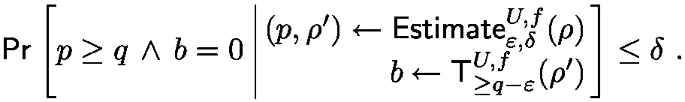
$\textsf{Estimate}_{\varepsilon ,\delta }^{U,f}$ has quantum circuit complexity $O(|f| \cdot \frac{1}{\varepsilon } \log \frac{1}{\delta })$ given oracle access to $U := \sum _{r \in R} |{r}{\rangle }\!{\langle }{r}|\otimes U(r)$.

We denote by $\textsf{Threshold}_{\gamma ,\varepsilon ,\delta }$ the quantum algorithm which runs $\textsf{Estimate}$ and outputs 1 if its output is at least $\gamma$, and 0 otherwise.

We recall the state repair theorem of [11].

Theorem 3

(State repair, [11]). Let $\textsf{M}$ be an $(\varepsilon ,\delta )$-almost projective measurement on $\mathcal {H}$, let $\textsf{P}$ be an n-outcome projective measurement on $\mathcal {H}$, and let T be any positive integer. There is quantum procedure $\textsf{Repair}$ such that $\textsf{RepExpt}_T^{\textsf{M},\textsf{P}}$ (see Fig. 1) satisfies the following guarantee. For any state $\mathbf {\rho }$ on $\mathcal {H}$ and $(p,p') \leftarrow \textsf{RepExpt}_{T}^{\textsf{M},\textsf{P}}(\mathbf {\rho })$:

$$\begin{aligned} \textsf{Pr}_{}\left[ |p' - p| > 2\varepsilon \right] \le n(\delta + 1/T) + 4 \sqrt{\delta }. \end{aligned}$$

Moreover, $\textsf{Repair}$ has quantum circuit complexity O(T) given oracle access to $\textsf{P}$ and $\overline{\textsf{M}}$.

Fix $\textsf{M}$ to be the procedure $\textsf{Estimate}_{\varepsilon ,\delta }^{U,f}$ from Lemma 2, and for $r \in R$, denote by $\textsf{P}_r$ the binary measurement $(U_r^{\dagger } \varPi _{f(r,\cdot )} U_r, I - U_r^{\dagger } \varPi _{f(r,\cdot )} U_r)$. In [11] it is observed that Theorem 3 directly implies the following. If we choose a uniformly random sequence $(r_1,\ldots ,r_N) \in R^N$ and apply $\textsf{RepExpt}_{T}^{\textsf{M},\textsf{P}_{r_1}},\ldots , \textsf{RepExpt}_{T}^{\textsf{M},\textsf{P}_{r_N}}$ sequentially, the expected number of 1-outcomes for the $\textsf{P}_{r_i}$ is at least $p - O(\varepsilon N)$, where p is the prover’s success probability in the protocol.

For our application we will need to strengthen this result in two ways. First, we allow the sequence to be drawn from a more general distribution, even depending on prior measurement outcomes. Second, we require a strong concentration guarantee, which we obtain by showing that the number of successes dominates a binomial distribution of the appropriate parameters. The relevant experiment is given as $\textsf{MultiExpt}$ in Fig. 1. Note that the setting in [11] is obtained by choosing $D_s$ as the uniform distribution over R for all s.

Lemma 3

For each $s = 1,\ldots ,N$, let $D_{s}$ be a randomized function that takes an element of $(\mathbb {N} \times \{0,1\})^{s-1}$ and outputs $i_s \in \mathbb {N}$. Let $(\textsf{M}_{i})_{i \in \mathbb {N}}$ be a list of measurements.

For any state $\mathbf {\rho }\in \textbf{S}(\mathcal {A}\otimes \mathcal {Z})$, the following holds:

$$\begin{aligned} \textsf{Pr}_{S \leftarrow \textsf{MultiExpt}(\mathbf {\rho })}\left[ S< k\right] \le \textsf{Pr}_{}\left[ \sum _{i=1}^{N} Y_s < k\right] + N/T + O(\sqrt{\delta } + (N/T)^2)~, \end{aligned}$$

where the $(Y_s)_{s=1}^{N}$ are distributed as follows:

• 1. Apply $\textsf{Estimate}_{\varepsilon ,\delta }^{U,f}$ to $\mathbf {\rho }$, obtaining outcome $p_0$. Let $\alpha := p_0 - 2\varepsilon N$.

• 2. For each $s \in [N]$, sample $Y_s$ from a Bernoulli distribution with parameter

  $$\begin{aligned} \zeta := \min _{|v\rangle \in \textrm{im}(\varPi _{\ge \alpha }^{U,f})} \min _{\begin{array}{c} \textbf{i} \in \mathbb {N}^{s-1} \\ \textbf{b} \in \{0,1\}^{s-1} \end{array}} \mathbb {E}_{i_s \leftarrow D_s(\textbf{i},\textbf{b})} \textsf{Pr}_{}\left[ \textsf{M}_{i_s} (|{v}{\rangle }\!{\langle }{v}|) \rightarrow 1 \right] ~. \end{aligned}$$

Proof

By Theorem 3, for each $s \in [N]$ it holds that

$$\begin{aligned} \textsf{Pr}_{}\left[ p_{s} < p_{s-1} - 2\varepsilon \right] \le 2/T + O(\sqrt{\delta })~. \end{aligned}$$

Denote by E the event that, for any $s \in [N]$, $p_{s} < p_{s-1} - 2\varepsilon$. By a union bound,

$$ \textsf{Pr}_{}\left[ E\right] \le 2N/T + O(N\sqrt{\delta } + (N/T)^2)~. $$

Now consider the following hybrid experiment:

• $\textsf{Hyb}^{\textsf{P}}_T$:

  • 1. Apply $\textsf{Estimate}$, obtaining outcome $p_0$.

  • 2. For $s = 1, \ldots , N$:

    • (a) Apply $\textsf{Estimate}$, obtaining outcome $p_s$.

    • (b) Apply $\textsf{T}_{\ge p_s - \varepsilon }^{U,f}$, and postselect on obtaining outcome 1.

    • (c) Sample $(i_s,\textsf{M}_{}) \leftarrow D_s(i_1,b_1,\ldots ,i_{s-1},b_{s-1})$, and measure $b_s \leftarrow \textsf{M}_{}$.

    • (d) Run $\textsf{Repair}_{T}[\textsf{Estimate},\textsf{M}_{i}](b_s,p_s)$.

By Lemma 2, in each iteration s, $\textsf{T}_{\ge p_s - \varepsilon }^{U,f}$ yields outcome 1 with probability at least $1-\delta$. Hence by gentle measurement, $d(\textsf{MultiExpt},\textsf{Hyb}) = O(N \sqrt{\delta })$. Switching to $\textsf{Hyb}$, it holds by definition of $\zeta$ that

$$\begin{aligned} \textsf{Pr}_{\textsf{Hyb}}\left[ b_s = 1 \mid \lnot E, i_1,b_1,\ldots ,i_{s-1},b_{s-1}\right] \ge \zeta ~. \end{aligned}$$

Therefore the distribution of $(\sum _{s=1}^{N} b_s \mid \lnot E)$ induced by $\textsf{Hyb}$ stochastically dominates $\sum _{s=1}^N Y_s$; that is, for all k,

Since $\textsf{Pr}_{}\left[ A\right] \le \textsf{Pr}_{}\left[ A | B\right] \textsf{Pr}_{}\left[ B\right]$, we have that

$$\begin{aligned} \textsf{Pr}_{\textsf{Hyb}}\left[ \sum _{s=1}^{N} b_s< k\right]&\le \frac{\textsf{Pr}_{}\left[ \sum _{s=1}^N Y_s< k\right] }{\textsf{Pr}_{\textsf{Hyb}}\left[ E\right] } \\&\le \textsf{Pr}_{}\left[ \sum _{s=1}^N Y_s < k\right] + 2N/T + O(N\sqrt{\delta } + (N/T)^2) ~. \end{aligned}$$

The lemma then follows by trace distance.    $\square$

5.2 Description of the Extractor

For a measurement channel $\textsf{M}_{}:\textbf{S}(\mathcal {A}) \rightarrow \textbf{S}(\mathcal {A}\otimes \mathcal {O})$, we denote by $\overline{\textsf{M}_{}} \in U(\mathcal {A}\otimes \mathcal {O}\otimes \mathcal {B})$ some unitary dilation of $\textsf{M}_{}$. We denote by $\underline{\textsf{M}_{}} :\textbf{S}(\mathcal {A}\otimes \mathcal {B}) \rightarrow \textbf{S}(\mathcal {A}\otimes \mathcal {O}\otimes \mathcal {B})$ a projective dilation of $\textsf{M}_{}$, given by

where $\{|i\rangle \}_i$ is a basis for $\mathcal {O}$. All of our procedures and correctness analyses are independent of the choice of dilation, and we assume that the circuit complexity of $\overline{\textsf{M}_{}},\underline{\textsf{M}_{}}$ is linear in the circuit complexity of $\textsf{M}_{}$.

We now describe the extractor, which is a measurement channel $\textsf{Extract}_{i,\nu } :\textbf{S}(\mathcal {A}\otimes \mathcal {Z}) \rightarrow \textbf{S}(\mathcal {A}\otimes \mathcal {Z}\otimes \mathcal {O})$, where $\mathcal {Z}= (\mathcal {Z}_1,\ldots ,\mathcal {Z}_t,\mathcal {W}_{t+1})$ are the prover’s output registers. Recall that we model the prover as a sequence of unitaries $U_{1},\ldots ,U_{t}$.

For $i \in [t]$, denote by $U^{(i)} :R_{i} \times \cdots \times R_{t} \rightarrow U(\mathcal {A}\otimes \mathcal {Z}_{i+1} \otimes \cdots \otimes \mathcal {Z}_{t} \otimes \mathcal {W}_{t+1})$ the map

$$\begin{aligned} U^{(i)}(r_i,\ldots ,r_t) = U_t(r_t) \cdots U_{i}(r_{i})~. \end{aligned}$$

For $i \in [t], \textbf{r} = (r_1,\ldots ,r_{i-1}) \in R_1 \times \cdots \times R_{i-1}$, let $f^{(i)}_{(\textbf{r})} :(R_{i} \times \cdots \times R_{t}) \times (Z_{1} \times \cdots \times Z_{t} \times W_{t+1}) \rightarrow \{0,1\}$ denote the function $f^{(i)}_{(\textbf{r})}(r_i,\ldots ,r_t,z_1,\ldots ,z_t,w_{t+1}) := V(z_1,r_1,\ldots ,z_t,r_t,w_{t+1})$.

$\textsf{Extract}_{t,\nu }(r_1,\ldots ,r_{t-1})$ is simply the [11] extractor, modified to sample $r_t$ without replacement:

Lemma 4

$\textsf{Extract}_{i,\nu }$ is a circuit of size $P(t,k,\log (1/\delta ),1/\nu ) \cdot (ck)^{t-i}$ for some polynomial P and constant c. In particular, if $k = O(1)$, $t = O(\log n)$, $\delta = 2^{-\lambda }$ and $\nu = 1/\textsf{poly}\,(\lambda )$ then $\textsf{Extract}_{\nu } = \textsf{Extract}_{1,\nu }$ is a polynomial-size quantum circuit.

Proof

Let P be a polynomial (with positive coefficients) such that for any i,

$$\begin{aligned} |\textsf{Extract}_{i,\nu }| \le P(t,k,\log (1/\delta ),1/\beta ,1/\nu ) + k \cdot 2|\textsf{Extract}_{i+1,\nu '}|~. \end{aligned}$$

Such a polynomial exists by Lemma 2 and Theorem 3. Let c be a constant such that $P(1,1,1,1,2) \le c \cdot P(1,1,1,1,1)$. The circuit size of $\textsf{Extract}_{i,\nu }$ is then bounded by

$$\begin{aligned}&P(t,k,\log (1/\delta ),1/\beta ,1/\nu ) + k \cdot 2|\textsf{Extract}_{i+1,\nu '}| \\&\le P(t,k,\log (1/\delta ),1/\beta ,1/\nu ) + 2c^{t-i-1} k^{t-i} \cdot P(t,k,\log (1/\delta ),1/\beta ,\textstyle {\frac{1}{\nu } \cdot \frac{t-i}{t-i-1}}) \\&\le (ck)^{t-i} P(t,k,\log (1/\delta ),1/\beta ,1/\nu )~, \end{aligned}$$

since $\frac{t-i}{t-i-1} \le 2$ for all $i \in \{1, \ldots , t-1\}$.    $\square$

5.3 Correctness

The key lemma which establishes the correctness of the extractor is the following.

Lemma 5

Let $\textsf{Extract}'$ be as $\textsf{Extract}$, except that its output is 0 if $\textsf{Extract}$ outputs $\bot$ and

$$\begin{aligned} V_{i-1}(z_1,r_1,\ldots ,z_{i-1},r_{i-1},w_{i-1}) \end{aligned}$$

otherwise. Then for $\gamma := \sum _{j=i}^{t} \frac{k-1}{R_i} + \nu$ and all $\textbf{r} = (r_1,\ldots ,r_{i-1})$,

$$\begin{aligned}&d_{\textsf{comp}}^{\mathcal {A},\mathcal {Z},\mathcal {O}}(\underline{\textsf{Extract}}'_{i,\nu }(\textbf{r};\mathbf {\rho }),\underline{\textsf{Threshold}}_{\gamma ,\varepsilon ,\delta }^{U^{(i)},f^{(i)}_{\textbf{r}}}(\mathbf {\rho })) \\ \le ~&k^{t-i} \cdot (\beta + O(\beta ^2) + \textsf{poly}\,(\lambda ) \cdot \root 4 \of {\delta }) + \textsf{negl}\,(\lambda )~. \end{aligned}$$

Before proving the lemma, we discuss the intuition behind it and then show how to use it to prove Theorem 2. $\underline{\textsf{Extract}}'_{i,\nu }$ measures whether the extractor succeeds at the i-th level. $\underline{\textsf{Threshold}}_{\gamma ,\varepsilon ,\delta }^{U^{(i)},f^{(i)}_{\textbf{r}}}$ measures whether the prover’s success probability in the i-th round is at least $\gamma$. The lemma bounds the computational distinguishability of these measurements; in particular, it implies that if we first measure $\underline{\textsf{Threshold}}_{\gamma ,\varepsilon ,\delta }^{U^{(i)},f^{(i)}_{\textbf{r}}}$ and obtain an outcome $b \in \{0,1\}$, then the outcome of applying $\underline{\textsf{Extract}}'_{i,\nu }$ to the post-measurement state is also b with all but inverse polynomial probability. Hence to determine whether $\underline{\textsf{Extract}}'_{i,\nu }$ will succeed it suffices to measure $\underline{\textsf{Threshold}}_{\gamma ,\varepsilon ,\delta }^{U^{(i)},f^{(i)}_{\textbf{r}}}$; the complexity of the latter does not grow with decreasing i.

We note that it is crucial that Lemma 5 bounds the distinguishability of these measurements and not simply the probability that they produce different outcomes when applied in sequence. While gentle measurement allows one to move from the latter property to the former, this incurs a square-root loss in the bound. Compounding this loss over $\log n$ rounds would make the bound trivial.

Proof

(Theorem 2). Let $P^* = (U_{1},\ldots ,U_{t}, \rho )$ be an adversary for $\varPi _t$. By Lemma 2, $\mathbb {E}[\textsf{Estimate}_{\varepsilon ,\delta }^{U^{(1)},f^{(1)}}(\rho )] = \textsf{Pr}_{}\left[ \langle P^*, V_t \rangle \rightarrow 1\right]$. Hence by Proposition 1,

$$\begin{aligned} \textsf{Pr}_{}\left[ \textsf{Threshold}_{\gamma ,\varepsilon ,\delta }^{U^{(1)},f^{(1)}}(\rho ) \rightarrow 1\right] \ge \textsf{Pr}_{}\left[ \langle P^*, V_t \rangle \rightarrow 1\right] - \gamma . \end{aligned}$$

It follows by Lemma 5 that

$$\begin{aligned} \textsf{Pr}_{}\left[ \textsf{Extract}'_{1,\nu /2} \rightarrow 1\right] \ge \textsf{Pr}_{}\left[ \langle P^*, V_t \rangle \rightarrow 1\right] - \kappa - \nu \end{aligned}$$

for $\kappa := \sum _{i=1}^{t} \frac{k-1}{|R_i|}$ and since $\beta = \nu /2k^t$. The theorem follows by noting that, by definition, the probability that $\textsf{Extract}$ succeeds is equal to the probability that $\textsf{Extract}'$ outputs 1.    $\square$

Proof

We argue the inductive step. The base case follows by a similar (simpler) argument.

Consider a hybrid extractor $\textsf{Hyb}_1$ in which we replace Steps 3f and 4 with

• 3f’. If $b' = 1$, add $(r_i \mapsto \bot )$ to W.

• 4’. Output 1 if $|W| = k$, else 0.

By last-round collapsing, $d_{\textsf{comp}}^{\mathcal {A},\mathcal {Z},\mathcal {O}}(\textsf{Extract}'_{i,\gamma ,\varepsilon },\textsf{Hyb}_1) = \textsf{negl}\,(\lambda )$.

Observe that after removing the measurement of $\mathcal {W}_i$ in $\textsf{Extract}'$, Steps 3d,3e and 3g are equivalent to an invocation of $\underline{\textsf{Extract}}'_{i+1,\nu '}$. We can now invoke the inductive hypothesis. Specifically, we consider another hybrid extractor $\textsf{Hyb}_2$, in which we replace Steps 3d to 3g with the following:

• If $b = 1$, measure $b' \leftarrow \underline{\textsf{Threshold}}_{\gamma '-\varepsilon ,\varepsilon ,\delta }^{U_{\textbf{r}},f_{\textbf{r}}}$. If $b' = 1$, add $(r_i \rightarrow \bot )$ to W.

By induction and the triangle inequality, $d(\textsf{Hyb}_1,\textsf{Hyb}_2) \le k^{t-i} \cdot (\varepsilon + O(\varepsilon ^2) + \textsf{poly}\,(\lambda ) \cdot \root 4 \of {\delta } + \textsf{negl}\,(\lambda ))$.

$\textsf{Hyb}_3$ is obtained from $\textsf{Hyb}_2$ by replacing Step 5.3 with

• 5.3’ If $b = 1$, add $(r_i \rightarrow \bot )$ to W.

If $b = 1$, then by Lemma 2, $\textsf{Pr}_{}\left[ b' = 1\right] \ge 1 - \delta$. Hence by gentle measurement, $d^{\mathcal {A},\mathcal {Z},\mathcal {O}}(\textsf{Hyb}_2,\textsf{Hyb}_3) = O(k \sqrt{\delta })$. We write out $\textsf{Hyb}_3$ in full, simplifying where possible.

Consider now the j-th iteration of the outer loop. We compute the quantity $\zeta$ from Lemma 3. Let $|v\rangle \in \textrm{im}(\varPi _{\ge \alpha }^{U^{(i)},f^{(i)}_{\textbf{r}}})$. Then

So by Proposition 1,

$$\begin{aligned} \textsf{Pr}_{r_i \leftarrow R_{i} \setminus \textrm{Supp}{W}}\left[ \underline{\textsf{Threshold}}_{\gamma ',\varepsilon ,\delta }^{U^{(i+1)},f^{(i+1)}}(U_{i}(r_i)|v\rangle ) \rightarrow 1\right] \ge \alpha - \frac{k-1}{|R_i|} - \gamma '. \end{aligned}$$

Since we abort if $p_0 < \gamma$, by our choice of $\varepsilon$ we have that $\alpha - \frac{k-1}{|R_i|} \ge \gamma ' + \frac{\nu }{2t}$. Hence $\zeta \ge \nu /2t$.

Then by Lemma 3, the probability that b is never set to 1 is at most

$$\begin{aligned} (1 - \nu /2t)^{N} + O(N(1/T + \sqrt{\delta })) \le \beta ^2/2k + O(N\sqrt{\delta } + \beta ^4/k^2) \end{aligned}$$

given our choice of N. Hence the probability that $p_0 \ge \gamma$ and $\textsf{Hyb}_3$ outputs 0 is at most $\beta ^2/2 + O(kN\sqrt{\delta } + \beta ^4)$. By gentle measurement,

$$\begin{aligned} d^{\mathcal {A},\mathcal {Z},\mathcal {O}}(\underline{\textsf{Hyb}}_3,\underline{\textsf{Threshold}}_{\gamma ,\varepsilon ,\delta }^{U^{(i)},f^{(i)}_{\textbf{r}}}) \le \beta + O(\sqrt{kN}\root 4 \of {\delta } + \beta ^2). \end{aligned}$$

The lemma then follows by the triangle inequality.    $\square$

6 Collapsing Hash Function Families

In the following, we show that the hash functions $\textsf{Hash}_{\textbf{A}}(\textbf{x}) = \textbf{A} \cdot \textbf{x} \bmod q$, indexed by the matrix $\textbf{A}$, are collapsing and even when $\textbf{A}$ is “folded” with coefficients being small units in the base ring.

6.1 Definitions

We recall the definition of a hash function family and the desired properties.

Definition 7

(Hash Function Family). Let $\ell , k \in \textsf{poly}\,(\lambda )$. A hash function family $\textsf{Hash} = (\textsf{Setup}, \textsf{H})$ from $\mathcal {X} ^\ell$ to $\mathcal {Y} ^h$ consists of a PPT $\textsf{Setup}$ algorithm and a deterministic polynomial-time $\textsf{H}$ algorithm. The $\textsf{Setup}$ algorithm inputs a security parameter $1^\lambda$ and outputs the public parameters $\textsf{pp}$. The $\textsf{H}$ algorithm inputs $\textsf{pp}$ and a preimage $\textbf{x} \in \mathcal {X} ^\ell$. It outputs an image $\textbf{y} \in \mathcal {Y} ^h$. When it is clear from the context, we omit the input $\textsf{pp}$ and write $\textbf{y} = \textsf{H}(\textbf{x})$.

We define below the notion of collapsing for hash functions [25].

Definition 8

(Collapsing). Let $\ell , k \in \textsf{poly}\,(\lambda )$ and $\mathcal {W} \subseteq \mathcal {X}$. Let $\textsf{Hash} = (\textsf{Setup}, \textsf{H})$ be a hash function from $\mathcal {X} ^\ell$ to $\mathcal {Y} ^h$. We say that $\textsf{Hash}$ is collapsing over $\mathcal {W}^\ell$ if for any efficient (quantum) adversary A

$$ \left|\textrm{Pr}\left[ {\textsf{Collapsing}^{0}_A(1^\lambda ) = 1}\right] - \textrm{Pr}\left[ {\textsf{Collapsing}^{1}_A(1^\lambda ) = 1}\right] \right| \le \textsf{negl}\,(\lambda ), $$

where the experiment $\textsf{Collapsing}^{b}_A$ is defined as follows:

$\underline{\textsf{Collapsing}^{b}_A(1^\lambda ):}$

• 1. Sample $\textsf{pp}$ using the $\textsf{Setup} (1^\lambda )$ algorithm and send it over to A.

• 2. A replies with a classical bitstring y and a quantum state on a register $\mathcal {X}$.

• 3. Let $U_{\textsf{H}, y}$ be the unitary that acts on $\mathcal {X}$ and a fresh ancilla, and CNOTs into the fresh ancilla the bit that determines whether the output of $\textsf{H}(\cdot )$ equals y and the input belongs to $\mathcal {W}^\ell$. Apply $U_{\textsf{pp}, y}$, measure the ancilla, and apply $U_{\textsf{pp}, y}^\dagger$.

• 4. If the output of the measurement is 0, then abort the experiment. Else proceed.

• 5. If $b = 0$ do nothing.

• 6. If $b = 1$ measure the register $\mathcal {X}$ in the computational basis, discard the result.

• 7. Return to A all registers and output whichever bit A outputs.

Note that the security experiment $\textsf{Collapsing}^{b}_A$ in the definition of collapsing is a quantum algorithm. It is often easier to work with the classical security notion of somewhere-statistically binding (SSB), defined below, which is known to imply collapsing.

Definition 9

(Somewhere-Statistically Binding). Let $h, \ell \in \textsf{poly}\,(\lambda )$ and $\mathcal {W} \subseteq \mathcal {X}$. A hash function family $\textsf{Hash} = (\textsf{Setup}, \textsf{H})$ from $\mathcal {X} ^\ell$ to $\mathcal {Y} ^h$ is said to be somewhere-statistically binding (SSB) over $\mathcal {W}^\ell$ if there exists a PPT $\textsf{BSetup}$ algorithm such that the following hold:

• The $\textsf{BSetup}$ algorithm inputs a security parameter $1^\lambda$ and an index $i \in \mathbb {Z}_\ell$. It outputs the public parameters $\textsf{pp}$.

• For all $i \in \mathbb {Z}_\ell$, the distributions $\textsf{Setup} (1^\lambda )$ and $\textsf{BSetup} (1^\lambda , i)$ are computationally indistinguishable.

• For all $i \in \mathbb {Z}_\ell$,

  $$\begin{aligned} \textrm{Pr}{ \left[ \exists ~\textbf{x}_0, \textbf{x}_1 \in \mathcal {W}^\ell : x_{0,i} \ne x_{1,i} \wedge \textsf{H}(\textsf{pp}, \textbf{x}_0) = \textsf{H}(\textsf{pp}, \textbf{x}_1)\right. \,\left| \,\left. \textsf{pp} \leftarrow \textsf{BSetup} (1^\lambda , i)\right] \right. }&\\ \le \textsf{negl}\,(\lambda ). \end{aligned}$$

Lemma 6

([1, 18]). Let $\textsf{Hash} = (\textsf{Setup}, \textsf{H})$ be a hash function family from $\mathcal {X} ^\ell$ to $\mathcal {Y} ^h$ and $\mathcal {W} \subseteq \mathcal {X}$. If $\textsf{Hash}$ is SSB over $\mathcal {W}^\ell$, then $\textsf{Hash}$ is collapsing over $\mathcal {W}^\ell$.

6.2 Bounded Homomorphic Public-Key Encryption

We recall the notion of public-key encryption. Note that we define a variant of public-key encryption with perfect correctness.

Definition 10

(Public-Key Encryption). A public-key encryption $(\textsf{Gen}, \textsf{Enc}, \textsf{Dec})$ consists of a key generation algorithm $\textsf{Gen}$ that takes as input the security parameter $1^\lambda$ and returns a key pair $(\textsf{pk}, \textsf{sk})$. The encryption algorithm $\textsf{Enc}$ takes as input $\textsf{pk}$ and a message m an produces a ciphertext c. We require that for all $\lambda \in \mathbb {N}$, all $(\textsf{pk}, \textsf{sk})$ in the support of $\textsf{Gen} (1^\lambda )$ and all messages m, it holds that $\textsf{Dec}(\textsf{sk}, \textsf{Enc}(\textsf{pk}, m)) = m$.

To prove the security of the hash function family $f_{\textbf{A}}$ we assume the existence of a bounded linearly homomorphic encryption scheme, that we define in the following.

Definition 11

($(\ell ,\beta )$-Bounded Linearly Homomorphic Encryption over $\mathcal {R}_q^h$). Let $h,q \in \mathbb {N}$. An encryption scheme $(\textsf{Gen}, \textsf{Enc}, \textsf{Dec})$ is $(\ell ,\beta )$-bounded linearly homomorphic over $\mathcal {R}_q^h$ if the following hold:

• (Ciphertext Indistinguishability) For a uniformly sampled key pair $(\textsf{pk}, \textsf{sk}) \leftarrow \textsf{Gen} (1^\lambda )$, and for all bits $b\in \{0,1\}$ it holds that the following distributions are computationally indistinguishable:

  

• (Bounded Homomorphism) For all key pairs $(\textsf{pk}, \textsf{sk})$ in the support of $\textsf{Gen} (1^\lambda )$, all bits $(b_1, \dots , b_\ell )\in \{0,1\}^\ell$, all ciphertexts $(\textbf{c}_1, \dots , \textbf{c}_\ell )\in \mathcal {R}_q^{h \times \ell }$ in the support of $(\textsf{Enc}(\textsf{pk}, b_1), \dots , \textsf{Enc}(\textsf{pk}, b_\ell ))$, and all vectors $\textbf{x} \in \mathcal {R}^\ell$ where $\left\| \textbf{x}\right\| \le \beta$, it holds that:

  $$ \textsf{Dec}(\textsf{sk}, (\textbf{c}_1,\dots , \textbf{c}_\ell )\cdot \textbf{x} \bmod q) = \sum _{i=1}^\ell b_i \cdot \textbf{x}_i. $$

Examples of encryption schemes that satisfy the above property are NTRU [12, 23] (for $h=1$) and Regev encryption based on (Ring)-LWE [17, 21] (for $h > 1$).

6.3 A Fold-Collapsing Hash Function

Let $h, t \in \mathbb {N}$, $\ell = 2^t$, $i \in \left\{ 0,1,\ldots ,t\right\}$, and $(r_j)_{j \in [i]]} \in \mathcal {R}^i$. Define $\ell _i := \ell /2^i = 2^{t-i}$. For any matrix $\textbf{A} _i \in \mathcal {R}_q^{h \times \ell _i}$, we denote by $(\textbf{A} _{i,0}, \textbf{A} _{i,1}) \in (\mathcal {R}_q^{h \times \ell _{i+1}})^2$ an arbitrary fixed partitioning of the columns of $\textbf{A}$ into two disjoint sets of columns of identical cardinality. Similarly, for any vector $\textbf{x}_i \in \mathcal {R}^{\ell _i}$, we denote by $(\textbf{x} _{i,0}, \textbf{x} _{i,1}) \in (\mathcal {R}_q^{\ell _{i+1}})^2$ the partitioning of $\textbf{x}$ induced by that of $\textbf{A}$. In Fig. 2 we define a hash function family $\textsf{Hash}_i := \textsf{Hash}[h,\ell ,(r_j)_{j \in [i]}]$ from $\mathcal {X} ^{\ell _i}$ to $\mathcal {Y} ^h$.

Fig. 2.

Construction of hash function families $\textsf{Hash}_i$ from $\mathcal {X} ^{\ell _i}$ to $\mathcal {Y} ^h$, where $\ell _i := \ell /2^i = 2^{t-i}$. For $i = 0$, we denote the family by $\textsf{Hash}_0 = \textsf{Hash}[h,\ell ]$.

We are now ready to show that the hash function as defined above is SSB, generalizing a Theorem from [1]. As an immediate corollary, we obtain that the hash function is also collapsing.

Lemma 7

(Collapsing). Let $\beta _0 \in \mathbb {R}$. Let $\mathcal {W}_0 := \left\{ x \in \mathcal {R}: \left\| x\right\| \le \beta _0 \right\}$. If there exists an $(\ell , \beta _0)$-bounded linearly homomorphic encryption over $\mathcal {R}_q^h$, then $\textsf{Hash}[h,\ell ]$ is SSB over $\mathcal {W}_0$.

Proof

Let $(\textsf{Gen}, \textsf{Enc}, \textsf{Dec})$ be an $(\ell , \beta _0)$-bounded linearly homomorphic encryption over $\mathcal {R}_q^h$. Let $\textbf{A}$ be a uniformly sampled hash key. We define $\ell$ hybrid distributions where we gradually substitute the columns of $\textbf{A}$ with encryptions of 0. That is, in the i-th hybrid, the key of the hash function consists of

$$ \left( \textbf{c}_1, \dots , \textbf{c}_{i} , \textbf{B} _i \right) $$

where and . It is easy to show that the hybrids of each neighbouring pair are computationally indistinguishable by the ciphertext indistinguishability of the encryption scheme. Note that, in the $\ell$-th hybrid, the hash key consists of a concatenation of encryption of 0.

We will now show that the hash function defined in the $\ell$-th hybrid is SSB, and the lemma statement will follow. We define $\textsf{BSetup} (1^\lambda , i)$ to be identical to the distribution above, except that we substitute the i-th column of the key with . The two distributions are computationally indistinguishable by another application of ciphertext indistinguishability. We now show that there does not exist a pair $(\textbf{x}_0, \textbf{x}_1) \in \mathcal {W}_0^{2\ell }$ such that $\textsf{H}(\textbf{x}_0) = \textsf{H}(\textbf{x}_1)$ and $x_{0,i} \ne x_{1,i}$. Assume towards contradiction that it exists, then we have that

$$ \tilde{c} = (\textbf{c}_1, \dots , \textbf{c}_{\ell })\cdot \textbf{x}_0 = (\textbf{c}_1, \dots , \textbf{c}_{\ell })\cdot \textbf{x}_1 \bmod q. $$

By the $(\ell , \beta _0)$-bounded linear homomorphism of the encryption scheme, it holds that $\tilde{c}$ decrypts to two different $x_{0,i}$ and $x_{1,i}$. This contradicts the correctness of the scheme.    $\square$

Next we show that the function remains collapsing even if we fold the hashing key by linear combinations with short units. We refer to this property as fold-collapsing.

Lemma 8

(Fold-Collapsing). Let $\beta _i \in \mathbb {R}$, $i \in \mathbb {Z}_t$, $r_{i+1} \in \mathcal {R}^{\times }$ be a unit with $\left\| r_{i+1}\right\| = 1$, $\mathcal {W}_i := \left\{ x \in \mathcal {R}: \left\| x\right\| \le \beta _i \right\}$, $\mathcal {W}_{i+1} := \left\{ x \in \mathcal {R}: \left\| x\right\| \le \gamma _\mathcal {R}^{-1} \cdot \beta _i \right\}$, $\textsf{Hash}_i := \textsf{Hash}[h,\ell ,(r_j)_{j \in [i]}] = (\textsf{Setup} _i, \textsf{H}_i)$, and $\textsf{Hash}_{i+1} := \textsf{Hash}[h,\ell ,(r_j)_{j \in [i+1]}] = (\textsf{Setup} _{i+1}, \textsf{H}_{i+1})$. If $\textsf{Hash}_i$ is SSB over $\mathcal {W}_i^{\ell _i}$, then $\textsf{Hash}_{i+1}$ is SSB over $\mathcal {W}_{i+1}^{\ell _{i+1}}$.

Proof

Since $\textsf{Hash}_i$ is SSB over $\mathcal {W}_i^{\ell _i}$, there exists a PPT algorithm $\textsf{BSetup} _i$ such that

• 1. $\textsf{BSetup} _i$ inputs $1^\lambda$ and $j \in \mathbb {Z}_{\ell _i}$ and outputs $\textsf{pp}$.

• 2. For any $j \in \mathbb {Z}_{\ell _i}$, $\textsf{Setup} _i(1^\lambda )$ and $\textsf{BSetup} _i(1^\lambda , j)$ are computationally indistinguishable.

• 3. For any $j \in \mathbb {Z}_{\ell _i}$,

  $$ \textrm{Pr}{\,\left[ \textsf{BAD}(i,j)\right. \,\left| \,\left. \textbf{A} _i \leftarrow \textsf{BSetup} _i(1^\lambda , j)\right] \right. } \le \textsf{negl}(\lambda ) $$

  where $\mathsf {BAD(i,j)}$ is defined as the following event:

  $$ \left\{ \exists ~ \textbf{x}_{i,0}, \textbf{x}_{i,1} \in \mathcal {W}_i^{\ell _i}: x_{i,0,j} \ne x_{i,1,j} \wedge \textbf{A} _i \cdot \textbf{x}_{i,0} = \textbf{A} _i \cdot \textbf{x}_{i,1} \bmod q\right\} . $$

We construct a PPT algorithm $\textsf{BSetup} _{i+1}$ which, on input $j' \in \mathbb {Z}_{\ell _{i+1}}$, samples $b \in \{0,1\}^{}$, runs $\textsf{BSetup} _i$ on $j = j' + b \cdot \ell _{i+1}$ to obtain $\textbf{A} _i$, and returns $\textbf{A} _{i+1} := r_{i+1} \cdot \textbf{A} _{i,0} + \textbf{A} _{i,1} \bmod q$. By Property 2 above, we clearly have that $\textsf{Setup} _{i+1}(1^\lambda )$ and $\textsf{BSetup} _{i+1}(1^\lambda , j')$ are computationally indistinguishable for all $j' \in \mathbb {Z}_{\ell _{i+1}}$.

Fix any $j \in \mathbb {Z}_{\ell _{i}}$ and $j' \in \mathbb {Z}_{\ell _{i+1}}$ satisfying $j = j' \bmod \ell _{i+1}$, any $\textbf{A} _i \in \textsf{BSetup} _i(1^\lambda , j)$, any $\textbf{A} _{i+1} = r_{i+1} \cdot \textbf{A} _{i,0} + \textbf{A} _{i,1} \bmod q \in \textsf{BSetup} _{i+1}(1^\lambda , j')$, and any $\textbf{x}_{i+1,0}, \textbf{x}_{i+1,1} \in \mathcal {W}_{i+1}^{\ell _{i+1}}$ satisfying $\textbf{A} _{i+1} \cdot \textbf{x}_{i+1,0} = \textbf{A} _{i+1} \cdot \textbf{x}_{i+1,1} \bmod q$. Define $\textbf{x}_{i,0} := (r_{i+1} \cdot \textbf{x}_{i+1,0}, \textbf{x}_{i+1,0})$ and $\textbf{x}_{i,1} = (r_{i+1} \cdot \textbf{x}_{i+1,1}, \textbf{x}_{i+1,1})$.

Note that $\left\| \textbf{x}_{i+1,0}\right\| \le \gamma _\mathcal {R}^{-1} \cdot \beta _i$ and $\left\| \textbf{x}_{i+1,1}\right\| \le \gamma _\mathcal {R}^{-1} \cdot \beta _i$. Clearly $\left\| \textbf{x}_{i,0}\right\| \le \beta _i$ and $\left\| \textbf{x}_{i,1}\right\| \le \beta _i$. In other words, we have $\textbf{x}_{i,0}, \textbf{x}_{i,1} \in \mathcal {W}_{i}^{\ell _{i}}$.

Since $\textbf{A} _{i+1} \cdot \textbf{x}_{i+1,0} = \textbf{A} _{i+1} \cdot \textbf{x}_{i+1,1} \bmod q$, we have

$$\begin{aligned} \textbf{A} _{i+1} \cdot \textbf{x}_{i+1,0}&= \textbf{A} _{i+1} \cdot \textbf{x}_{i+1,1} \bmod q, \\ (r_{i+1} \cdot \textbf{A} _{i,0} + \textbf{A} _{i,1}) \cdot \textbf{x}_{i+1,0}&= (r_{i+1} \cdot \textbf{A} _{i,0} + \textbf{A} _{i,1}) \cdot \textbf{x}_{i+1,1} \bmod q, \\ \textbf{A} _i \cdot (r_{i+1} \cdot \textbf{x}_{i+1,0}, \textbf{x}_{i+1,0})&= \textbf{A} _i \cdot (r_{i+1} \cdot \textbf{x}_{i+1,1}, \textbf{x}_{i+1,1}) \bmod q, \\ \textbf{A} _i \cdot \textbf{x}_{i,0}&= \textbf{A} _i \cdot \textbf{x}_{i,1} \bmod q. \end{aligned}$$

Furthermore, if $x_{i+1,0,j'} \ne x_{i+1,1,j'}$, we have $x_{i,0,j'} \ne x_{i,1,j}$ and $x_{i,0,j' + \ell _{i+1}} \ne x_{i,1,j' + \ell _{i+1}}$ since $r_{i+1} \in \mathcal {R}^\times$ is a unit in $\mathcal {R}$.

Suppose $\textsf{Hash}_{i+1}$ is not SSB over $\mathcal {W}_{i+1}^{\ell _{i+1}}$, then there exists $j' \in \mathbb {Z}_{\ell _{i+1}}$ such that

$$ \textrm{Pr}{\,\left[ \textsf{BAD}(i+1, j')\right. \,\left| \,\left. \textbf{A} _{i+1} \leftarrow \textsf{BSetup} _{i+1}(1^\lambda , j')\right] \right. } $$

is non-negligible. Consequently, by the above derivation, the average

$$\begin{aligned}&\frac{1}{2} \cdot \textrm{Pr}{\,\left[ \textsf{BAD}(i,j')\right. \,\left| \,\left. \textbf{A} _i \leftarrow \textsf{BSetup} _i(1^\lambda , j')\right] \right. } \\ +&\frac{1}{2} \cdot \textrm{Pr}{\,\left[ \textsf{BAD}(i,j'+\ell _{i+1})\right. \,\left| \,\left. \textbf{A} _i \leftarrow \textsf{BSetup} _i(1^\lambda , j'+\ell _{i+1})\right] \right. } \end{aligned}$$

is non-negligible. We conclude that there exists $j \in \left\{ j', j'+\ell _{i+1}\right\} \subseteq \mathbb {Z}_{\ell _{i}}$ such that

$$ \textrm{Pr}{\,\left[ \textsf{BAD}(i,j)\right. \,\left| \,\left. \textbf{A} _i \leftarrow \textsf{BSetup} _i(1^\lambda , j)\right] \right. } $$

is non-negligible, contradicting Property 3 above.    $\square$

Note that the elements $r_j$ of the sets R defined in Proposition 2 satisfy the requirements in Lemma 8.

References

Albrecht, M.R., Cini, V., Lai, R.W.F., Malavolta, G., Thyagarajan, S.A.K.: Lattice-based snarks: publicly verifiable, preprocessing, and recursively composable. In: Dodis, Y., Shrimpton, T. (eds.) Advances in Cryptology–CRYPTO 2022. Lecture Notes in Computer Science, vol. 13508, pp. 102–132. Springer, Cham (2022). https://doi.org/10.1007/978-3-031-15979-4_4
Albrecht, M.R., Lai, R.W.F.: Subtractive sets over cyclotomic rings. In: Malkin, T., Peikert, C. (eds.) CRYPTO 2021. LNCS, vol. 12826, pp. 519–548. Springer, Cham (2021). https://doi.org/10.1007/978-3-030-84245-1_18
Attema, T., Cramer, R.: Compressed \(\varSigma \)-protocol theory and practical application to plug & play secure algorithmics. In: Micciancio, Daniele, Ristenpart, Thomas (eds.) CRYPTO 2020. LNCS, vol. 12172, pp. 513–543. Springer, Cham (2020). https://doi.org/10.1007/978-3-030-56877-1_18
Attema, T., Cramer, R., Kohl, L.: A compressed \(\varSigma \)-protocol theory for lattices. In: Malkin, T., Peikert, C. (eds.) CRYPTO 2021, Part II. LNCS, vol. 12826, pp. 549–579. Springer, Heidelberg, Virtual Event (Aug 2021). https://doi.org/10.1007/978-3-030-84245-1_19
Attema, T., Fehr, S.: Parallel repetition of \((k_1,\dots , k_{\mu })\)-special-sound multi-round interactive proofs. Cryptology ePrint Archive, Report 2021/1259 (2021). https://ia.cr/2021/1259
Ben-Sasson, E., Chiesa, A., Spooner, N.: Interactive oracle proofs. In: Hirt, M., Smith, A. (eds.) TCC 2016. LNCS, vol. 9986, pp. 31–60. Springer, Heidelberg (2016). https://doi.org/10.1007/978-3-662-53644-5_2
Bootle, J., Cerulli, A., Chaidos, P., Groth, J., Petit, C.: Efficient zero-knowledge arguments for arithmetic circuits in the discrete log setting. In: Fischlin, M., Coron, J.-S. (eds.) EUROCRYPT 2016. LNCS, vol. 9666, pp. 327–357. Springer, Heidelberg (2016). https://doi.org/10.1007/978-3-662-49896-5_12
Bootle, J., Chiesa, A., Sotiraki, K.: Sumcheck arguments and their applications. In: Malkin, T., Peikert, C. (eds.) CRYPTO 2021. LNCS, vol. 12825, pp. 742–773. Springer, Cham (2021). https://doi.org/10.1007/978-3-030-84242-0_26
Bootle, J., Lyubashevsky, V., Nguyen, N.K., Seiler, G.: A non-PCP approach to succinct quantum-safe zero-knowledge. In: Micciancio, D., Ristenpart, T. (eds.) CRYPTO 2020. LNCS, vol. 12171, pp. 441–469. Springer, Cham (2020). https://doi.org/10.1007/978-3-030-56880-1_16
Bünz, B., Bootle, J., Boneh, D., Poelstra, A., Wuille, P., Maxwell, G.: Bulletproofs: short proofs for confidential transactions and more. In: 2018 IEEE Symposium on Security and Privacy, pp. 315–334. IEEE (2018). https://doi.org/10.1109/SP.2018.00020
Chiesa, A., Ma, F., Spooner, N., Zhandry, M.: Post-quantum succinct arguments: Breaking the quantum rewinding barrier. In: FOCS, pp. 49–58. IEEE (2021)
Hoffstein, J., Pipher, J., Silverman, J.H.: NTRU: a ring-based public key cryptosystem. In: Buhler, J.P. (ed.) ANTS 1998. LNCS, vol. 1423, pp. 267–288. Springer, Heidelberg (1998). https://doi.org/10.1007/BFb0054868
Kilian, J.: A note on efficient zero-knowledge proofs and arguments (extended abstract). In: 24th ACM STOC, pp. 723–732. ACM Press (1992). https://doi.org/10.1145/129712.129782
Lai, R.W.F., Malavolta, G., Ronge, V.: Succinct arguments for bilinear group arithmetic: practical structure-preserving cryptography. In: Cavallaro, L., Kinder, J., Wang, X., Katz, J. (eds.) ACM CCS 2019, pp. 2057–2074. ACM Press (2019). https://doi.org/10.1145/3319535.3354262
Liu, Q., Zhandry, M.: Revisiting post-quantum fiat-Shamir. In: Boldyreva, A., Micciancio, D. (eds.) CRYPTO 2019. LNCS, vol. 11693, pp. 326–355. Springer, Cham (2019). https://doi.org/10.1007/978-3-030-26951-7_12
Lombardi, A., Ma, F., Spooner, N.: Post-quantum zero knowledge, revisited (or: How to do quantum rewinding undetectably). CoRR abs/2111.12257 (2021)
Lyubashevsky, V., Peikert, C., Regev, O.: On ideal lattices and learning with errors over rings. In: Gilbert, H. (ed.) EUROCRYPT 2010. LNCS, vol. 6110, pp. 1–23. Springer, Heidelberg (2010). https://doi.org/10.1007/978-3-642-13190-5_1
Ma, F.: Quantum-secure commitments and collapsing hash functions. https://www.cs.princeton.edu/fermim/talks/collapse-binding.pdf (2020)
Marriott, C., Watrous, J.: Quantum arthur-merlin games. In: Computational Complexity Conference, pp. 275–285. IEEE (2004)
Micali, S.: CS proofs (extended abstracts). In: 35th FOCS, pp. 436–453. IEEE (1994). https://doi.org/10.1109/SFCS.1994.365746
Regev, O.: On lattices, learning with errors, random linear codes, and cryptography. In: Gabow, H.N., Fagin, R. (eds.) 37th ACM STOC, pp. 84–93. ACM Press (2005). https://doi.org/10.1145/1060590.1060603
Shor, P.W.: Algorithms for quantum computation: discrete logarithms and factoring. In: 35th FOCS, pp. 124–134. IEEE (1994). https://doi.org/10.1109/SFCS.1994.365700
Stehlé, D., Steinfeld, R.: Making NTRU as secure as worst-case problems over ideal lattices. In: Paterson, K.G. (ed.) EUROCRYPT 2011. LNCS, vol. 6632, pp. 27–47. Springer, Heidelberg (2011). https://doi.org/10.1007/978-3-642-20465-4_4
Unruh, D.: Quantum proofs of knowledge. In: Pointcheval, D., Johansson, T. (eds.) EUROCRYPT 2012. LNCS, vol. 7237, pp. 135–152. Springer, Heidelberg (2012). https://doi.org/10.1007/978-3-642-29011-4_10
Unruh, D.: Computationally binding quantum commitments. In: Fischlin, M., Coron, J.-S. (eds.) EUROCRYPT 2016. LNCS, vol. 9666, pp. 497–527. Springer, Heidelberg (2016). https://doi.org/10.1007/978-3-662-49896-5_18
Winter, A.: Coding theorem and strong converse for quantum channels. IEEE Trans. Inf. Theory 45(7), 2481–2485 (1999). https://doi.org/10.1109/18.796385, https://doi.org/10.1109
Zhandry, M.: Schrödinger’s pirate: how to trace a quantum decoder. In: Pass, R., Pietrzak, K. (eds.) TCC 2020. LNCS, vol. 12552, pp. 61–91. Springer, Cham (2020). https://doi.org/10.1007/978-3-030-64381-2_3
Acknowledgments
The authors thank Fermi Ma for many helpful discussions throughout the development of this work.
G.M. is partially supported by the German Federal Ministry of Education and Research BMBF (grant 16K15K042, project 6GEM) and funded by the Deutsche Forschungsgemeinschaft (DFG, German Research Foundation) under Germany\(\acute{}\)s Excellence Strategy - EXC 2092 CASA - 390781972.
Author information
Authors and Affiliations
Corresponding author
Editor information
Editors and Affiliations
Rights and permissions
Copyright information
© 2022 The Author(s), under exclusive license to Springer Nature Switzerland AG
About this paper
Cite this paper
Lai, R.W.F., Malavolta, G., Spooner, N. (2022). Quantum Rewinding for Many-Round Protocols. In: Kiltz, E., Vaikuntanathan, V. (eds) Theory of Cryptography. TCC 2022. Lecture Notes in Computer Science, vol 13747. Springer, Cham. https://doi.org/10.1007/978-3-031-22318-1_4
Download citation
DOI: https://doi.org/10.1007/978-3-031-22318-1_4
Published:
Publisher Name: Springer, Cham
Print ISBN: 978-3-031-22317-4
Online ISBN: 978-3-031-22318-1
eBook Packages: Computer ScienceComputer Science (R0)