
Abstract
Development of hydraulic fracture in lab tests is accompanied by a significant pressure drop in fracturing fluid. This is not normally observed in the field. The pressure drop suggests the presence of a stage of unstable fracture growth in the laboratory samples. The paper shows that unstable fracture growth is produced by interaction between the fracture and free sample surfaces that are parallel to the fracture. This is another difference from the field situation on top of the scale difference, since in the field the presence of a nearby free surfaces parallel and close to the hydraulic fractures is a rare occurrence. This finding is important in analysing the results of laboratory experiments and developing methods of their upscaling.
Access provided by Autonomous University of Puebla. Download conference paper PDF
Keywords
1 Introduction
Pressure monitoring of fracturing fluid in the process of hydraulic fracture propagation in the field shows at most a slight pressure drop (not exceeding the recorded pressure fluctuations) corresponding to the time of hydraulic fracture initiation (e.g. [1, 2]). Opposite to this, the laboratory experiments on hydraulic fracturing show considerable pressure drop at the fracture initiation [3, 4] (in some cases almost to zero pressure, [5,6,7,8,9] as also shown in the experiments described below).
While small pressure drops at the time of onset of the field hydraulic fracture can be attributed to the difference between the pressure required to initiate the fracture and the pressure needed to maintain the fracture growth, the considerable pressure drops observed in the laboratory experiments require the presence of an unstable stage of fracture propagation. Unstable fracture propagation, that is propagation under reduced pressure, requires considerable increase of the stress intensity factor with fracture size, R. If one assumes that the hydraulic fracture propagates under the pressure p of fracturing fluid applied to the whole fracture surface, then the growth will be unstable as the stress intensity factor \(K_{I} \propto p\sqrt R\) increases as a square root of the crack size. However, the almost instantaneous pressure drop measured at the pump suggests that the fractures have grown faster than the fracturing fluid could fill the fracture. (This would not be the case in the field as the hydraulic fractures there are large enough to ensure their filling with the fracturing fluid.) Therefore, the unstable fracture growth is produced by the pressure concentrated at the fracture area of the order of the borehole diameter. In the simplest case when the fracture is modelled as a 2D crack this corresponds to the situation of the crack growing under the action of a pair of concentrated forces of magnitude \(F = 2al/L\), where a is the borehole radius, l is the length of the pressurised part of the borehole (between packers), L is the sample length. Such a loading leads to the stress intensity factor \(K_{I} \propto p/\sqrt R\) decreasing as a square root of the crack size.
This paper investigates the above mechanism of fracture growth instability assuming that the unstable fracture growth is induced by interaction of the fracture with the sample free surfaces that are parallel to the fracture. (The other pairs of the sample faces are assumed to produce little effect on the fracture propagation.)
2 Unstable Fracture Growth in Laboratory Experiments
Two tests [10] were conducted on 100 mm cubic samples of mortar (cement:sand:water = 1:1:0.4). The sand particle sizes were under 0.15 mm. The properties of mortar samples are: density ρ = 2.3 g/cm3, Young’s modulus (dynamic) E = 27.9 GPa, dynamic Poisson’s ratio \(\nu = 0.19\).
The experiments and equipment are shown in Fig. 1 [10]. Silicon oil of 97.77 cp viscosity was used as fracturing fluid; it was pumped using a GDS high pressure pump with volume control. Figure 2a shows schematics of the fracture-produced loading, a model of borehole of radius a = 2 mm and working (fracture-produced) length of l = 30 mm. Sample size is L = 100 mm. The produced hydraulic fracture is indicated by a circle (broken line). The pressure changes with time are shown in Fig. 2b, c. The sample was also pre-loaded vertically (z-axis, Figs. 1b, 2a) with steel loading platens to ensure that the fracture propagates vertically. During the tests the acoustic emission was recorded by the AE sensors hosted by the upper loading platen, Fig. 1b. The accumulated number of pulses is plotted in Fig. 2b, c. The displacement was measured on the face parallel to the crack using the DIC with Phantom stereo-vision high speed cameras, Fig. 1a.
Hydraulic fracture growth proceeds with local interruptions and overlapping resulting in formation of bridges distributed across the whole fracture and constricting the fracture opening [8, 9]. The effective stiffness k of the system of bridges relating stress that opens the fracture and fracture surface displacement, \(\sigma = k{\Delta }u/2\), where \({\Delta }u\) is the average fracture opening can be estimated from the displacement measurements as follows. Since the stage is considered when the fracture almost traverses the sample, the average displacement related to the average fracture opening, \({\Delta }u/2\) is approximately equal to the average displacement of the sample surface. The average opening stress \(\sigma\) is taken as approximately equal to the peak borehole pressure since the fracturing fluid moves inside the fracture. The effective bridge stiffness produces a characteristic length [8,9,10], so-called constriction length \(\lambda = E/k\), where E is the Young’s modulus of the sample material (mortar).
The peak pressure, the (average) fracture opening at the peak as well as the estimated effective bridge stiffnesses and the constriction lengths are summarised in Table 1. It is seen that the constriction length is almost 2 orders of magnitude greater than the sample size, which suggests that the effect of bridges can be neglected, and the fracture can be modelled as a conventional crack with non-interacting faces.

Laboratory experiments on hydraulic fracture [10]: (a) Experimental set-up; (b) tested sample with a hydraulic fracture between two vertical loading platens; the upper loading platen also hosts the AE sensors; (c) schematics of the model of borehole.

Results of laboratory experiments on hydraulic fracture (of radius R) in a cubic sample of size L = 100 mm [10]: (a) schematics of the fracture-produced loading in the experiment; only pressurised part of the borehole is shown (length l = 30 mm, diameter 2a = 4 mm); the acoustic emission sensors are located between the upper loading platen and the sample; (b) results of test 1; (c) results of test 2, pump pressure (kPa) and total number of AE events versus time (s).
3 Mechanism of Unstable Fracture Growth in Laboratory Experiments
In the above experiments the size, 2R, of the produced fractures is of the order of the sample size, L = 100 mm, Figs. 1b, 2a. This is much greater than the borehole radius a = 2 mm. This suggests a simplified way of modelling the fracture growth by considering it as a 2D crack opened at the centre by a pair of 2D concentrated forces F (such a crack is shown in Fig. 3a) representing the opening action of the pressurised borehole.
Here p is the peak pressure in the borehole, a is the borehole radius, l is the pressurised part of the borehole, L is the sample size. In this 2D modelling the total force 2pal is referred to the whole sample thickness, L.
The unstable growth of such a crack can be produced by interaction with a free surface parallel to the crack [11, 12]; as soon as the crack length reaches a critical value (corresponds to the minimum of the stress intensity factor) the stress intensity starts increasing with the crack size and the crack growth becomes unstable.
In the case under consideration the fracture is located at the centre of the sample, therefore the closest configuration would be the crack located at the centre of a free strip with free surfaces, Fig. 3a. For this configuration the stress intensity factor reads:
Function f(s) is tabulated in [13]. It is also shown to have two simple asymptotics: \(f\left( s \right)\sim \left( {1 - s} \right)^{3/2}\) as \(s \to 0\) and \(f\left( s \right)\sim \sqrt {3\pi } s^{3/2} /2\) as \(s \to 1\). This allows putting forward the following approximation that incorporates these two asymptotics:
Comparison of Eq. (3) with the numerical values given by [13] shows that the average relative error over 7 points is 4%.
Dependence (2), (3) is shown in Fig. 3b. It is seen that as R increases the stress intensity factor reaches minimum and then increases. The critical crack size, \(R_{cr}\), obviously corresponds to the minimum, \(dK_{I} /dR = 0\). This gives:
The unstable fracture propagation commences when the pressure p is such that
where \(K_{Ic}\) is the fracture toughness of the material.

Unstable fracture growth due to interaction of with free surfaces: (a) crack at the centre of a strip with free surfaces; (b) normalised stress intensity factor versus the normalised crack size.
4 Discussion
-
1.
The obtained criterion of unstable fracture propagation (4), (5) can be interpreted by introducing a characteristic microscopic fracture length \(l_{m}\) which is the minimum size of the fracturing element. In the case of crack propagation it is an equivalent of the process zone length, but instead of considering the non-linear processes within this zone (which might well be material specific) we will use a simplified approach [14,15,16] by considering the magnitude of the singular stress at distance \(l_{m}\) from the crack tip, Fig. 4, and equating it to the minimum tensile strength \(\sigma_{t}\) to express the criterion of fracture propagation. (In [14] the non-singular terms were also taken into account which lead to the expression of the scale effect in fracture toughness; in the simplified model considered in this paper only singular terms are used.)
Subsequently, the criterion of unstable fracture propagation (4), (5) expressed in terms of the minimum tensile strength \(\sigma_{t}\) reads:
The fracture starts from the borehole pressurised to pressure p, at the point with the minimum strength, which is \(\sigma_{t}\). Given that the stress concentration at the borehole surface is p, one finds that \(\sigma_{t} = p\). From here, using criterion (6) one can estimate the characteristic microscopic length \(l_{m} \sim 7 \cdot 10^{ - 3} {\text{mm}}\). This is close to the lower limit of Portland cement grain sizes, \(10^{ - 3} - 10^{ - 1} {\text{ mm}}\) (e.g., [17]). This suggests that fracturing of mortar involves the scale of cement grains (that is the smallest scale) while the presence of heterogeneities of larges sizes leads to complex fracture surface geometry at the microscale. In particular, the fracture becomes patchy with local overlapping and formation of bridges distributed all over the fracture, Fig. 5 [10].
-
2.
The above approach ignores the effect of the other pairs of sample surfaces. The pair of surfaces subjected to vertical load is in contact with the loading platens and hence cannot be free due to the contact friction. The other pair of surfaces that is normal to the fracture is not included because the model is two dimensional. A planned 3D modelling will be directed towards investigating the effect of fracture geometry and interaction with all sample surfaces.
Fig. 4. 
The concept of crack growth criterion based on the introduction of characteristic microscopic length \(l_{m}\). The coordinate frame corresponds to that of Fig. 3a.
Fig. 5. 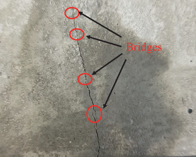
Bridges (local interruptions and overlapping) observed on the fracture trace [10].


5 Conclusions
Laboratory experiments on hydraulic fracture are often used to investigate fracking in the field. It is conventionally accepted that the major distinction between the laboratory experiments and the field situation is the scale difference, which is to be addressed by upscaling. This paper demonstrates that there exists another important difference—the presence of the sample free surfaces in the laboratory tests, which are not normally present in the field. (The faults or joints do not represent free surfaces as their faces are in contact due to in situ compressive stresses.)
Interaction between the growing fracture and the free surfaces oriented parallel to the fracture turns initially stable fracture growth into unstable well before the fracturing fluid is able to fill the fracture and thus ensures the continuation of fracture growth. This leads to the sharp drop of the pressure not observed in the field.
The analysis also shows that fractures in mortar samples grow by breaking microscopic elements at the cement grain scale. This produces patchy fracturing leading to local overlapping and formation of distributed bridges [8,9,10].
References
Jeffrey, R.G., Bunger, A.P., Lecampion, B., Zhang, X, Chen, Z.R., van As, A. Allison, D.P. de Beer, W., Dudley, J.W., Siebrits, E, Thiercelin, M, Mainguy, M.: Measuring hydraulic fracture growth in naturally fractured rock. SPE 124919, 1–19 (2009)
Zhang, Y., Zhang, J., Yuan, B., Yin, S.: In-situ stresses controlling hydraulic fracture propagation and fracture breakdown pressure. J. Petrol. Sci. Eng. 164, 164–173 (2018)
Hayashi, K., Haimson, B.C.: Characteristics of shut-in curves in hydraulic fracturing stress measurements and determination of in situ minimum compressive stress. J Geophys. Res. 96(B11), 18311–18321 (1991)
Ning, L., Shicheng, Z., Yushi, Z., Xinfang, M., Shan, W., Yinuo, Z.: Experimental analysis of hydraulic fracture growth and acoustic emission response in a layered formation. Rock Mech. Rock Eng. 51, 1047–1062 (2018)
AlTammar, M.J., Sharma, M.M., Manchanda, R.: The effect of pore pressure on hydraulic fracture growth: an experimental study. Rock Mech. Rock Eng. 51, 2709–2732 (2018)
Hampton, J.C., Hu, D., Matzar, L., Gutierrez, M.: Cumulative volumetric deformation of a hydraulic fracture using acoustic emission and micro-CT imaging. ARMA 14-7041 (2014)
Bunger, A.P., Kear, J., Dyskin, A.V., Pasternak, E.: Interpreting post-injection acoustic emission in laboratory hydraulic fracturing experiments. Proc. ARMA 14-6973 (2014)
Dyskin, A.V., Pasternak, E., He, J., Lebedev, M., Gurevich, B.: The role of bridge cracks in hydraulic fracturing. In: Proceedings of the 10th International Conference on Structural Integrity and Failure (SIF2016). Adelaide, Australia, Paper #6 (2016)
He, J., Pasternak, E., Dyskin, A.V.: Bridges outside fracture process zone: their existence and effect. Eng. Fract. Mech. 225, 106453 (2020)
He, J., Pasternak, E., Dyskin, A.V.: Monitoring of hydraulic fracture using photogrammetry and acoustic emission. Abstract and presentation for seminar series: Mechanics of Rocks and Structural Materials. University of Western Australia, 23 July (2020)
Dyskin, A.V., Germanovich, L.N.: Model of rockburst caused by cracks growing near free surface. In: Rockbursts and Seismicity in Mines, vol. 93, pp. 169–175 (1993)
Germanovich, L.N., Dyskin, A.V.: Fracture mechanisms and instability of openings in compression. Int. J. Rock Mech. Min. Sci. 37(1), 263–284 (2000)
Tada, H., Paris, P.C., Irwin, R.I.: The Stress Analysis of Cracks Handbook, 2nd edn. Paris Production Inc., St Luis, Missouri (1985)
Dyskin, A.V.: Crack growth criteria incorporating non-singular stresses: Size effect in apparent fracture toughness. Int. J. Fracture 83, 191–206 (1997)
Dyskin, A.V., Pasternak, E.: Asymptotic analysis of fracture propagation in materials with rotating particles. Eng. Fract. Mech. 150, 1–18 (2015)
Dyskin, A.V., Pasternak, E., Esin, M.: Multiscale rotational mechanism of fracture propagation in geomaterials. Phil. Mag. 95(28–30), 3167–3191 (2015)
Ferraris, C.F., Hackley, V.A., Avilés, A.I.: Measurement of particle size distribution in Portland cement powder: analysis of ASTM Round Robin studies. Cem. Concr. Aggregates 26(2), 1–11 (2004)
Acknowledgement
AVD and EP acknowledge the support of the Australian Research Council through projects DP190103260 and LE17170100079.
Author information
Authors and Affiliations
Corresponding author
Editor information
Editors and Affiliations
Rights and permissions
Copyright information
© 2023 The Author(s), under exclusive license to Springer Nature Switzerland AG
About this paper

Cite this paper
Dyskin, A.V., Pasternak, E., He, J. (2023). A Mechanism of Unstable Growth of Hydraulic Fractures in Laboratory Experiments. In: Pasternak, E., Dyskin, A. (eds) Multiscale Processes of Instability, Deformation and Fracturing in Geomaterials. IWBDG 2022. Springer Series in Geomechanics and Geoengineering. Springer, Cham. https://doi.org/10.1007/978-3-031-22213-9_13
Download citation
DOI: https://doi.org/10.1007/978-3-031-22213-9_13
Published:
Publisher Name: Springer, Cham
Print ISBN: 978-3-031-22212-2
Online ISBN: 978-3-031-22213-9
eBook Packages: EngineeringEngineering (R0)