Concept of Relational Similarity Search

Abstract

For decades, the success of the similarity search has been based on a detailed quantification of pairwise similarity of objects. Currently, the search features have become much more precise but also bulkier, and the similarity computations more time-consuming. While the k nearest neighbours (kNN) search dominates the real-life applications, we claim that it is principally free of a need for precise similarity quantifications. Based on the well-known fact that a selection of the most similar alternative out of several options is a much easier task than deciding the absolute similarity scores, we propose the search based on an epistemologically simpler concept of relational similarity. Having arbitrary objects $q, o_1, o_2$ from the search domain, the kNN search is solvable just by the ability to choose the more similar object to q out of $o_1, o_2$ – the decision can also contain a neutral option. We formalise such searching and discuss its advantages concerning similarity quantifications, namely its efficiency and robustness. We also propose a pioneering implementation of the relational similarity search for the Euclidean spaces and report its extreme filtering power in comparison with 3 contemporary techniques.

This research was supported by ERDF “CyberSecurity, CyberCrime and Critical Information Infrastructures Center of Excellence” (No. CZ.02.1.01/0.0/0.0/16_019/ 0000822).

1 Introduction and Preliminaries

Efficient similarity search in complex objects, actions, and events is a central problem of many data processing tasks [1, 13, 15]. Geometric models of similarity are established as a basic and practically the only approach to an efficient similarity search [17]. They assume a domain of the searched objects D and a distance function $d: D \times D \mapsto \textbf{R}^+_0$ that quantifies the dissimilarity of two objects. Two basic types of similarity queries are the kNN(q) and range(q, r) queries, where $q \in D, k \in \textbf{N}, r \in \textbf{R}^+_0$. Having a searched dataset $X \subseteq D$ and a query object $q \in D$, kNN(q) queries search for k most similar objects $o \in X$ to q, and range(q, r) queries search for objects $o \in X$ within distance $d(q, o) \le r$. In this article, we focus on kNN(q) queries which are more user friendly since setting the k value is intuitive and does not require any knowledge of the searched space.

Most of the approaches to kNN(q) query executions maintain k distances d(q, o) between q and k closest objects o found during the query evaluation. Typically, they require plenty of expensive distance computations [7, 10, 11]. We claim that kNN(q) queries do not require most of the dissimilarity quantifications since they ask just for the ordered list of k objects $o \in X$.

We propose to replace most of the precise dissimilarity quantifications with possibly much simpler decisions on which of the objects $o_1, o_2 \in X$ is more similar to $q \in D$. These decisions can use several independent and domain-specific views. The similarity/relevance comparisons of 2 objects with respect to the referent are widely used, e.g., in active learning, and they are well discussed theoretically [3]. Yet, they are not directly used to speed up the similarity search, according to our best knowledge. We discuss advantages of this relational similarity search considering the evaluation efficiency, effectiveness, and robustness while preserving the applicability. We formalise the relational kNN similarity search and propose the implementation for high dimensional Euclidean spaces.

The rest of the article is organised as follows. Sect. 2 presents the concept of relational similarity, Sect. 3 describes the implementation of relational similarity for Euclidean spaces and the experiments, and Sect. 4 concludes the paper.

2 Similarity Quantifications vs. Relational Similarity

This article focuses on kNN(q) similarity queries, and we start with the simplest case of the 1NN(q) search for the most similar object $o \in X$ to q.

2.1 One Nearest Neighbour Search

Consider an intermediate state of the 1NN(q) query execution, i.e., the objects:

• q: the query object

• $o_{top} \in X$: the most similar object to q found so far

• $o \in X$: object that is checked whether forms a better answer than $o_{top}$

In this situation, search techniques based on similarity quantifications usually know the distance $d(q, o_{top})$ and evaluate d(q, o) to decide the more similar object to q out of $o_{top}$ and o. Evaluation of d(q, o) is generally expensive [4, 14, 17], and the only optimisation related to this paper is applicable to distance functions which do not decrease during d(q, o) evaluation: Since $d(q, o_{top})$ is known, object o is relevant just until d(q, o) is known to be bigger than $d(q, o_{top})$. Therefore, d(q, o) evaluation can be interrupted when $d(q, o) > d(q, o_{top})$ is guaranteed.

Fig. 1.

Three images during the 1NN(q) search: query image q, the answer candidate $o_{top}$, and image o from the dataset. Despite distances $d(q, o_{top}) \approx d(q, o)$, approaches to efficiently discard o as irrelevant to q exist and are used by humans. In this case, it is checking the contours of $q, o_{top}, o$, for instance.

Nevertheless, the question whether o provides a better query answer than $o_{top}$ is often much simpler than d(q, o) evaluation, as illustrated by Fig. 1. Here, we consider the image similarity search, though our ideas are applicable to various domains. Distances $d(q, o_{top}) = 79.8$ and $d(q, o) = 80.5$ provided in Fig. 1 are the actual distances of corresponding image visual descriptors DeCAF described in Sect. 3.1. The distances suggest that d(q, o) evaluation cannot be cut much before its end since the difference $d(q, o) - d(q, o_{top})$ is small. At the same time, image o with the bird is obviously irrelevant to the query image q, and this is quickly realised by humans. By an analogy, an efficient formal approach to choose the 1NN(q) query answer from $o_{top}$ and o should exist.

We inspire our thoughts by humans, who typically give a quick glimpse at each of the images $q, o_{top}, o$, trying to make a quick decision on which of $o_{top}, o$ is more similar to q. If the first glimpse is insufficient to decide, the human gives another glimpse at images $q, o_{top}, o$ trying to choose the more similar image to q, and then continues (if necessary) in this iterative process until making the decision. The conclusion can also be “I do not know” or “the similarities of $o_{top}$ and o to q are (almost) the same”.

To illustrate this iterative approach, we again consider Fig. 1 and a human who first focuses on the colours in the images, for instance. Colours of images $q, o_{top}, o$ in Fig. 1 cannot efficiently distinguish the suitability of $o_{top}$ and o as the 1NN(q) answer, so after no success with the first glimpse, the considered human gives another glimpse at all objects $q, o_{top}, o$. Let us assume that the humans’ second glimpse reveals o displaying a different object than q and $o_{top}$ since he/she focuses on the image contours. Therefore, he/she decides that $o_{top}$ forms a better 1NN(q) answer than o.

The iterative process of the human deciding on which of $o_{top}, o$ forms a better 1NN(q) answer is in a principal contrast with the similarity quantifications performed by contemporary similarity search techniques. Most of the data domains are nowadays associated with an expensive similarity function d, and both distances d(q, o) and $d(q, o_\textit{top})$ are evaluated (with the possible early termination of d(q, o) evaluation) whenever the relevance of $o \in X$ and $o_{top}$ with respect to q must be decided. Different approaches of humans and contemporary search engines motivate us to formalise the concept of the relational similarity search that follows the humans’ attitude.

2.2 Relational Similarity Search

Beside of the pairwise similarity quantification $d: D \times D \mapsto \textbf{R}^+_0$, we define function (the similarity relation) $\textit{simRel}: D \times D \times D \mapsto \{0, 1, 2\}$:

$$\begin{aligned} \textit{simRel}(q, o_1, o_2) = {\left\{ \begin{array}{ll} 1 &{} \text {similarity of }q, o_1\text { is bigger than the similarity of }q, o_2\\ 2 &{} \text {similarity of }q, o_1\text { is lower than the similarity of }q, o_2\\ 0 &{} \!\begin{aligned} &{} \text {similarity of }q, o_1\text { is the same as the similarity of }q, o_2, \\ &{} \text {or the difference in the similarities is as small as its} \\ &{} \text {proper investigation does not pay-off, and similarities} \\ &{} \text {can be treated arbitrarily} \end{aligned} \end{array}\right. } \end{aligned}$$

(1)

We propose the simRel evaluations according to the informal concept sketched by Algorithm 1. The actual simRel implementations should be dependent on the data domain as well as on the application, which is well captured by the doubled semantic of the equality $0 = \textit{simRel}(q, o_1, o_2)$. The applications preferring the search efficiency should implement the simRel in an approximate manner and return 0 in more cases than the applications requiring high search effectiveness. We have shown that the simRel captures the core of the 1NN(q) search. In the following, we propose an algorithm for the kNN(q) search.

2.3 The k Nearest Neighbour Search with the Relational Similarity

To achieve the best search efficiency, we assume an abstract simRel implementation and discuss the kNN search algorithm, first. Let us consider $q \in D$, and $o_1, o_2, o_3 \in X$ such that $0 = \textit{simRel}(q, o_1, o_2) = \textit{simRel}(q, o_2, o_3)$. In other words, $o_1$ and $o_2$ are interchangeable in their similarity to q, and so do objects $o_2$ and $o_3$. Notation suggests the transitivity of these equations, i.e., the deduction of the equality $\textit{simRel}(q, o_1, o_3) = 0$. Still, it does not hold, in general, so the kNN search algorithms have to deal with this non-transitivity.

We propose the search algorithm which starts to build the query answer $\textit{ans}(k\text {NN}(q))$ as a list of the most similar objects $o \in X$ found during the query execution. When $o \in X$ is asked whether it is one the k nearest neighbours of q, the non-transitivity of the equalities $0 = \textit{simRel}(q, o_1, o_2)$ motivates us to focus on objects $o_a \in \textit{ans}(k\text {NN}(q)){}$ such that $\textit{simRel}(q, o_a, o) \ne 0$. We start to check $\textit{ans}(k\text {NN}(q))$ from its end:

• If we find $o_1 \in \textit{ans}(k\text {NN}(q)){}$ such that $\textit{simRel}(q, o_1, o) = 2$, i.e., o matches the query object q better than $o_1$, we mark $o_1$ to be removed from $\textit{ans}(k\text {NN}(q))$.

• We remember the lowest position i of $o_1 \in \textit{ans}(k\text {NN}(q)){}: \textit{simRel}(q, o_1, o) = 2$. If $\textit{ans}(k\text {NN}(q))$ does not contain $o_2: \textit{simRel}(q, o_2, o) = 1$, i.e., $o_2$ matches q better than o, then o is inserted to $\textit{ans}(k\text {NN}(q))$ at position i.

• If $\textit{ans}(k\text {NN}(q))$ contains $o_2$ such that $\textit{simRel}(q, o_2, o) = 1$ and $o_2$ is at the position $i < k - 1$ (numbering from 0) of $\textit{ans}(k\text {NN}(q))$, we add o into $\textit{ans}(k\text {NN}(q))$ just after $o_2$.

• Finally, we delete as many of marked objects $o_1$ from the answer $\textit{ans}(k\text {NN}(q))$ as the answer size does not decrease below k.

An important case remains: If $\textit{ans}(k\text {NN}(q))$ contains just objects $o_a$ such that $\textit{simRel}(q, o_a, o) = 0$, we add o into list $\textit{objsUnknown}(q)$ of objects with an unknown relation to q. The way of $\textit{objsUnknown}(q)$ processing is application dependent, and we consider two variants. The search algorithm returns either $\textit{candSet}(q){} = \textit{ans}(k\text {NN}(q)){} \cup \textit{objsUnknown}(q){}$, or $\textit{candSet}(q)= \textit{ans}(k\text {NN}(q))$. The second option which ignores list $\textit{objsUnknown}(q)$ is suitable for the applications oriented on a high efficiency and just the relevance of query answers. In both cases, $\textit{candSet}(q)$ is processed sequentially, i.e., distances $d(q, o), o \in \textit{candSet}(q)$ are evaluated to return k most similar objects from $\textit{candSet}(q)$ as a query answer. It can be just an approximation of the precise answer. The whole relational kNN search is formalised by Algorithm 2.

3 Proof of Concept for Euclidean Spaces

The only goal of the simRel implementations is to algorithmize Eq. 1 for a specific application and domain D to provide a suitable trade-off between the evaluation efficiency, correctness, and the number of equalities $\textit{simRel}(q, o_1, o_2) = 0$. We assume that the simRel implementations should follow the humans’ behaviour, i.e., the smaller the difference in the similarities of $q, o_1$ and $q, o_2$, the longer time to decide the $\textit{simRel}(q, o_1, o_2)$ correctly, or return 0 to save time.

The concept of relational similarity has potential to improve various aspects of the similarity search. We present a simRel implementation to efficiently search high-dimensional Euclidean spaces with a low memory consumption and just a small decrease in the search effectiveness.

No ambition to improve the search effectiveness enables us to implement the simRel which approximates the search space $({\textbf {R}}^\lambda , \ell _2)$ – here $\ell _2$ is the Euclidean distance function and $\lambda$ is the length of vectors. Motivated by the humans’ abilities, we want to implement simRel($q, o_1, o_2$) in a way that the bigger the difference $|\ell _2(q, o_1) - \ell _2(q, o_2)|$, the more efficient simRel($q, o_1, o_2$) evaluation. Consequently, we want to capture as much information about each $o \in X$ in one number, then capture as much of the remaining information in the second number, etc. This informal description sufficiently fits the Principal component analysis (PCA) [12, 16], i.e., the transformation of vectors $o \in X$ of length $\lambda$ to the vectors $o^\textit{PCA(L)} \in {\textbf {R}}^L$ of length $L < \lambda$ such that the variance of values in coordinates of $o^\textit{PCA(L)}$ decreases with the coordinates’ index, and the shortened vector $o^\textit{PCA(L)}$ preserves as much of the information about o as possible. First coordinates of vectors $q^\textit{PCA(L)}$, $o_1^\textit{PCA(L)}$, $o_2^\textit{PCA(L)}$ thus often contain sufficient information to decide $\textit{simRel}(q, o_1, o_2)$.

Our $\textit{simRel}(q, o_1, o_2)$ implementation starts to evaluate $\ell _2(q^\textit{PCA(L)}, o_1^\textit{PCA(L)})$ and $\ell _2(q^\textit{PCA(L)}, o_2^\textit{PCA(L)})$ distances in parallel. During the evaluation, it checks which of the vectors $o_1^\textit{PCA(L)}$ and $o_2^\textit{PCA(L)}$ is currently closer to $q^\textit{PCA(L)}$ and how much. If one of the vectors $o_1^\textit{PCA(L)}$, $o_2^\textit{PCA(L)}$ is sufficiently closer to $q^\textit{PCA(L)}$ than the second one, we claim the result of $\textit{simRel}(q^\textit{PCA(L)}, o_1^\textit{PCA(L)}, o_2^\textit{PCA(L)})$. We use this result as the estimation of $\textit{simRel}(q, o_1, o_2)$.

Formally, we denote $o^\textit{PCA(L)}$[i] the value in the ith coordinate of $o^\textit{PCA(L)}$, and define:

$$\begin{aligned} \begin{aligned} \textit{difSqPref}(&q^\textit{PCA(L)}, o_1^\textit{PCA(L)}, o_2^\textit{PCA(L)}, \varOmega ) = \\ {}&\sum _{i = 0}^\varOmega \left( q^\textit{PCA(L)}[i] - o_1^\textit{PCA(L)}[i]\right) ^2 - \sum _{i = 0}^\varOmega \left( q^\textit{PCA(L)}[i] - o_2^\textit{PCA(L)}[i]\right) ^2 \end{aligned} \end{aligned}$$

(2)

We evaluate this function for each integer $\varOmega : 0 \le \varOmega < L$, and consider thresholds $t(\varOmega ) \in \textbf{R}_0^+$ which determine the stop conditions for the $\textit{simRel}(q, o_1, o_2)$ evaluation: we start with $\varOmega$ = 0 and use Eq. 2 as follows:

• If $\textit{difSqPref}(q^\textit{PCA(L)}, o_1^\textit{PCA(L)}, o_2^\textit{PCA(L)}, \varOmega ) > t(\varOmega )$, then simRel($q, o_1, o_2$) = 2

• If $\textit{difSqPref}(q^\textit{PCA(L)}, o_1^\textit{PCA(L)}, o_2^\textit{PCA(L)}, \varOmega ) < - t(\varOmega )$, then simRel($q, o_1, o_2$) = 1

• If $\varOmega = L - 1$, then simRel($q, o_1, o_2$) = 0, else increment $\varOmega$

The (non-optimised) simRel implementation which takes $t(\varOmega )$ thresholds as an input is formalised by Algorithm 3.

We learn thresholds $t(\varOmega )$ using Algorithm 2 which evaluates kNN(q) queries with random query objects on a sample of the dataset X and use the simRel implementation formalised by Algorithm 4. This simRel implementation does not use the thresholds $t(\varOmega )$ but learns them instead. First, it evaluates distances $\ell _2(q^\textit{PCA(L)}, o_1^\textit{PCA(L)})$ and $\ell _2(q^\textit{PCA(L)}, o_2^\textit{PCA(L)})$. Let us assume inequality $\ell _2(q^\textit{PCA(L)}, o_1^\textit{PCA(L)}) \le \ell _2(q^\textit{PCA(L)}, o_2^\textit{PCA(L)})$ – if it does not hold, the notation of $o_1$ and $o_2$ is swapped. For each $\varOmega : 0 \le \varOmega < L$, the simRel algorithm stores a list wit $[\varOmega ]$ of observed positive values difSqPref $(q^\textit{PCA(L)}, o_1^\textit{PCA(L)}, o_2^\textit{PCA(L)}, \varOmega )$. These values wit $[\varOmega ]$ are witnesses of the insufficiency of prefix of length $\varOmega$: while first $\varOmega$ coordinates of vectors (i.e. function difSqPref) suggests the inequality $\ell _2(q^\textit{PCA(L)}, o_1^\textit{PCA(L)}) > \ell _2(q^\textit{PCA(L)}, o_2^\textit{PCA(L)})$, the last coordinates $i: \varOmega< i < L$ of vectors change the relation to the final inequality $\ell _2(q^\textit{PCA(L)}, o_1^\textit{PCA(L)}) \le \ell _2(q^\textit{PCA(L)}, o_2^\textit{PCA(L)})$. When all the queries are evaluated, each $\textit{wit}[\varOmega ]$ is sorted and $t(\varOmega )$ is defined as a given percentile perc of wit $[\varOmega ]$. The percentile defines the trade-off between the simRel correctness, evaluation times and the number of the equalities $0 = \textit{simRel}(q, o_1, o_2)$: the bigger the perc, the longer and the more precise the simRel decisions with possibly more neutral assessments $0 = \textit{simRel}(q, o_1, o_2)$. In the experiments, we use the perc = 0.85. The whole approach to determine thresholds $t(\varOmega )$ is formalised by Algorithm 4, and a Java implementation of this article is provided upon request.

3.1 Test Data

We examine the DeCAF image visual descriptors [5] extracted from the Profiset image collection¹ to verify the simRel implementation. We use a subset of 1 million descriptors that are derived from the Alexnet convolutional neural network [6] as the data from the second-last fully connected layer (FC7). Each descriptor consists of a 4,096-dimensional vector of floating-point values that describes characteristic image features, so there is a correspondence 1 to 1 between images and descriptors. Pairwise similarities of the DeCAF descriptors are expressed by Euclidean distances.

3.2 PCA and Relational Similarity Search Implementation

The PCA defines vectors with the most of information in their first coordinates. The relational similarity $\textit{simRel}(q, o_1, o_2)$ is thus decided just by a short prefix of vectors $q^\textit{PCA(L)}$, $o_1^\textit{PCA(L)}$, $o_2^\textit{PCA(L)}$ in most of the cases, and we propose to store just prefixes of $o^\textit{PCA(L)}, o \in X$ in the main memory while the long descriptors o can be in the secondary storage. If the prefixes are insufficient to decide $\textit{simRel}(q, o_1, o_2)$, zero is returned. The proposed simRel implementation contains several sources of approximation errors, and we address the setting of parameters one by one to mitigate them. We consider 30NN(q) queries on 4,096-dimensional DeCAF descriptors. Reported statistics are the medians over 1,000 query evaluations with different query objects q selected in random. The ground-truth consists of 30 closest objects $o_{\textit{NN}} \in X$ to q as defined by $\ell _2$ distance function.

Table 1. Median accuracy of the 30NN(q) search in DeCAF descriptors shortened by the PCA to length L: $k'$ vectors are pre-selected in a shrunk space and refined

The first parameter to be fixed is length L of vectors shortened by the PCA, and we set it experimentally using the filter & refine paradigm: Having an object $q \in D$, we select $k'$ closest vectors $o^\textit{PCA(L)}$ to $q^\textit{PCA(L)}$ using the $\ell _2$ distances, find the corresponding vectors $o \in X$ to form $\textit{c}(q) \subseteq X$, and re-rank these o according to $\ell _2(q, o)$. Finally, we consider just 30 closest objects $o \in \textit{c}(q)$ and check how many of them are the true nearest neighbours from the ground-truth.

Table 1 provides the median search² accuracy for various L and $k'$. For instance, vectors shortened to just 24 dimensions are of a quality that the set $\textit{c}(q)$ of size 1,000 vectors (0.1 % of the dataset) contains 28 out of 30 (93.3 %) true nearest neighbours per median query object q. Since the proposed simRel implementation speeds up the search by efficient and quite accurate similarity comparisons, we use the simRel together with a high-quality approximation of DeCAF descriptors given by $L = 256$. Having $L = 256$, the $\textit{candSet}(q)$ of 100 vectors contains all 30 true nearest neighbours per median query, so in the following, we address 100NN(q) search in vectors $o^\textit{PCA(L)}, o \in X, L = 256$.

Fig. 2.

Early terminations of simRel evaluations. The first coordinate of vectors shortened by the PCA decides 511,850 simRel evaluations per median query (Color figure online)

3.3 Experimental Verification of the Relation Similarity Search

The simRel evaluations must be efficient to pay-off. We use just first 24 coordinates of vectors $o^\textit{PCA(L)}, o \in X$ with $4\text {B}$ precision per coordinate stored in the main memory. The memory occupation is thus $24 \cdot 4\text {B} = 96\text {B}$ plus ID per $o \in X$. We learn thresholds $t[\varOmega ]$ by Algorithms 2 and 4 evaluating a hundred 30NN(q) queries with different q than 1,000 tested and a sample of 100K objects $o \in X$.

Fig. 3.

Relative numbers early terminations of the simRel evaluations during the query execution after checking the ith coordinate of vectors (Color figure online)

Number of simRel evaluations during kNN(q) execution by Algorithm 2 can be almost $k \cdot |X|$, but this happens just if $\textit{simRel}(q, o_1, o_2) = 0$ for nearly all examined triplets. Figure 4a reports numbers of simRel evaluations during 100NN$(q^\textit{PCA(L)})$ search in the prefixes of 1M vectors $o^\textit{PCA(L)}$. All box plots in this paper depict the distribution of values over 1,000 randomly selected query objects. The simRel evaluation counts are from 1.027M to 35.23M with the quartiles 1.2M, 1.47M and 2.37M, respectively. The results are thus much better than the theoretical worst case of almost $100 \cdot 1\text {M} = 100\text {M}$ simRel evaluations.

The simRel implementation given by Algorithm 3 adaptively decides how many out of 24 coordinates to use for an efficient simRel decision. Figure 2 presents numbers of simRel terminations just after checking the ith coordinate of vectors $q^\textit{PCA(L)}$, $o_1^\textit{PCA(L)}$, $o_2^\textit{PCA(L)}$. Indexes i are on the x-axis, and y-axis depicts the number of simRel terminations. The only exception is the last grey box plot which represents the last stored coordinate of $o^\textit{PCA(L)}$: Since we are interested in the simRel result, we use two box plots here. The red right-most box plot, as well as the last grey box plot depict the numbers of simRel evaluations which use all 24 coordinates – the red box plot depicts the zero results of simRel computations, and the last grey box plot depicts non-zero results. The first coordinate of $q^\textit{PCA(L)}$, $o_1^\textit{PCA(L)}$, $o_2^\textit{PCA(L)}$ is sufficient to decide 513,133 simRel comparisons per median query – see the first box plot in Fig. 2. The first and third quartiles are 439,776 and 645,781, respectively, the minimum is 324,425 and the maximum is 999,756. Value simRel = 0 is returned in 456,929 evaluations per median query, as depicted by the red box plot. This statistic has a large variance over q: the first and third quartiles are 192,897 and 1.35M, respectively, the minimum is 4,272, and the maximum is 34.2M.

Figure 3 also reports the simRel terminations after checking the ith coordinate of vectors, but expressed relatively with respect to the number of simRel evaluations during the query execution. The first box plot depicts that 33.68 % of simRel evaluations performed during the median query execution are terminated just after the check of the first coordinate of $q^\textit{PCA(L)}$, $o_1^\textit{PCA(L)}$, $o_2^\textit{PCA(L)}$. This statistic also have a large variance, and ranges from 1.91 % to 93.74 % with the quartiles 21.65 %, 33.64 %, and 43.08 %. The relative number of equalities $0 = \textit{simRel}(q, o_1, o_2)$ during the query execution ranges from 0.42 % to 97.18 % with the quartiles 15.94 %, 31.04 %, and 57.30 % – see the red box plot in Fig. 3. We suppose that query objects with a large number of simRel = 0 are probably outlying objects, and we postpone their investigation for the future work. We emphasise that the prevalent early termination of simRel evaluations leading to flexible evaluation times figure the key advantage of the simRel in comparison with most of the traditional search techniques based on, for example, dimensionality reduction or hashing.

Fig. 4.

Statistics gathered during 100NN search in 1M dataset, distributions over 1,000 query objects q

Table 2. Comparison of the filtering power

Finally, we chain all steps and report results of Algorithm 2 evaluating 30NN queries in the original space of 4,096-dimensional DeCAF descriptors. The simRel implementation uses the first 24 coordinates of $o^\textit{PCA(L)}, L = 256$. First, we evaluate Algorithm 2 to return $\textit{candSet}(q){} = \textit{ans}(k\text {NN}(q)){} \cup \textit{objsUnknown}(q){}$, i.e., we also refine the objects with an unknown relation to q. Figure 4b illustrates that Algorithm 2 correctly finds 28 out of 30 true nearest neighbours per median query. Figure 4c reports $\textit{candSet}(q)$ sizes which express the only number of 4,096-dimensional descriptors from X that we access during the query execution and evaluate their $\ell _2$ distances to q. It ranges from 101 to 19,643, i.e., from 0.01 % to 1.96 % of the dataset, with the quartiles 524; 1,076; and 2,477. The median thus expresses that the simRel filters out 99.89 % of the 1M dataset, 1,076 objects remains, and 28 out of them are in the set of 30 true nearest neighbours – all for a median query object q.

Table 2 compares³ the filtering power of the simRel with 3 most powerful filtering techniques we have ever tried. The GHP_50_256 [8] and GHP_80_256 [9] techniques transform DeCAF descriptors to the bit-strings of length 256 bits in the Hamming space. In this space, they identify the $\textit{candSet}(q)$ which they re-rank to return 30 most similar objects $o \in \textit{candSet}(q){}$. The pivot permutation based index PPP-codes [11] stores distances to 24 reference objects (pivots) which is the only information used to identify the $\textit{candSet}(q)$ before its refinement. We set parameters of all examined techniques to produce $\textit{candSet}(q)$ with the median accuracy 28/30. However, the results of all techniques except of the simRel are simulations describing the minimum $\textit{candSet}(q)$ size implying this accuracy. The $\textit{candSet}(q)$ size must be set in advance in case of GHP_50_256, GHP_80_256, and PPP-codes, and no support for an estimation of a suitable $\textit{candSet}(q)$ size is provided. The numbers presented for these 3 techniques thus form just a theoretical optimum. On the contrary, the result of the simRel describes a real usage which requires no hidden knowledge. Having the same memory overhead as the PPP-codes and 3 times bigger overhead than the bit-strings, the filtering with the simRel is 3 times, 3.1 times, and 9.8 times more powerful than the filtering with GHP_50_256, GHP_80_256, and PPP-codes, respectively.

Proposed simRel implementation has an advantage of automatic adapting to particular query objects q, which causes a significant variance in the simRel evaluation times and numbers of simRel evaluations during the query execution. Conversely, plenty of search techniques execute the similarity queries with fixed parameters and no adaptation to particular query objects. It leads to wasting computational sources in case of easy-to-evaluate query objects, or a low-quality evaluation of difficult queries [10].

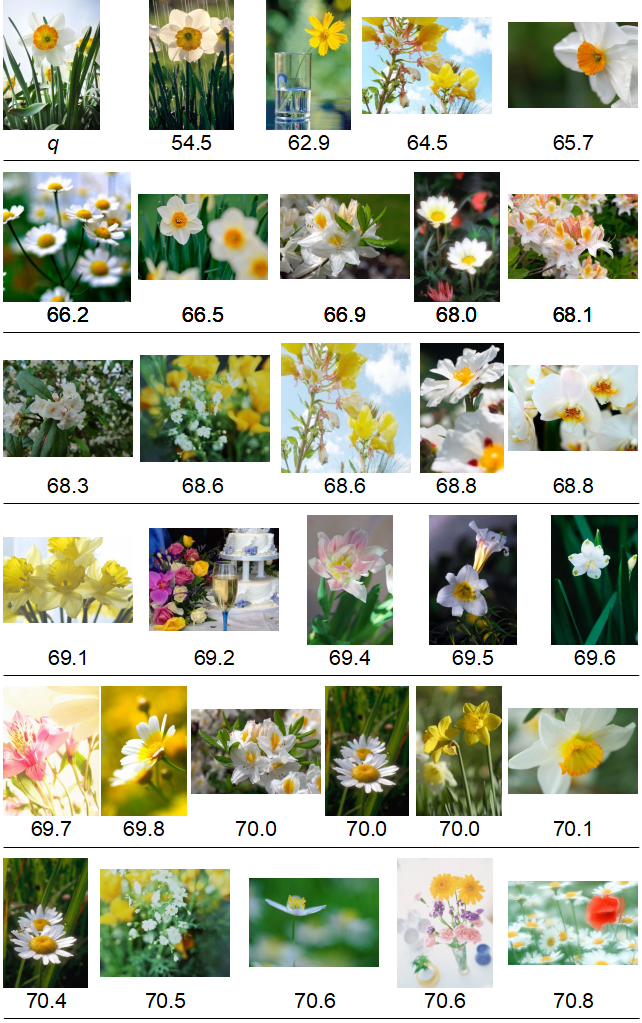
Finally, we examine the 30NN search with Algorithm 2 ignoring objects $\textit{objsUnknown}(q)$ with an unknown relation to q. The search accuracy of such search has median 10/30 and the third quartile 14/30, but the $\textit{candSet}(q)$ is pretty small with just 252 objects (0.0252 % of X) per median q. We visualise online⁴ the answer of typical quality to one 30NN query evaluated in this way. Its accuracy is 12/30 and it requires just 250 $\ell _2(q, o)$ evaluations to re-rank the $\textit{candSet}(q)$. We emphasise that the order of the images is given by full $\ell _2$ distances of the DeCAF descriptors depicted below each image. All answer images are relevant to q.

4 Conclusions

The content preserving features of contemporary digital data objects become more precise but also more voluminous and their similarity quantifications more computationally demanding. The partitioning techniques are not able to constrain the query response set sufficiently, and many distance computations are needed to get the result. We have proposed the relational similarity search to reduce the number of distance computations. In general, a large number of not necessary distance computations is eliminated by an efficient selection of a more similar data object out of two to the referent. We exemplify the approach by the search in a challenging high-dimensional Euclidean space and demonstrate the savings of 99.89 % distance computations per median query when finding 28 out of 30 nearest neighbours. The search algorithm can also be set to prefer the search efficiency at the cost of accuracy. In that case, we have observed the filtering of 99.9748 % of the dataset with the search accuracy of 33.3 % per median query, but still achieving a good answer relevance. In the future, we plan to implement the simRel in other domains, and combine the approach with the similarity indexes to efficiently search large datasets.

References

Amato, G., Falchi, F., Vadicamo, L.: Visual recognition of ancient inscriptions using convolutional neural network and fisher vector. ACM J. Comput. Cultural Heritage 9(4), 21:1–21:24 (2016)
Brázdil, J.: Dimensionality reduction methods for vector spaces. Master’s thesis, Masaryk University, Faculty of Informatics, Brno (2016). https://is.muni.cz/th/v9xlg/. Supervisor Pavel Zezula
Chang, R.: Are Hard Cases Vague Cases? Value Incommensurability: Ethics, Risk, and Decision-Making, pp. 50–70. Routledge, New York (2021)
Deza, M.M., Deza, E.: Encyclopedia of Distances, pp. 1–583. Springer, Heidelberg (2009). https://doi.org/10.1007/978-3-642-00234-2
Donahue, J., et al.: DeCAF: a deep convolutional activation feature for generic visual recognition. In: Proceedings of the 31th International Conference on Machine Learning, ICML, China, pp. 647–655 (2014)
Krizhevsky, A., Sutskever, I., Hinton, G.E.: ImageNet classification with deep convolutional neural networks. In: Advances in Neural Information Processing Systems 25, pp. 1097–1105. Curran Associates, Inc. (2012)
Mariachkina, I.: Experimental verification of a synergy of techniques for efficient similarity search in metric spaces (2022). https://is.muni.cz/th/m14as/. Bachelor’s thesis, Masaryk University, Faculty of Informatics, Brno, supervisor Vladimir Mic
Mic, V., Novak, D., Zezula, P.: Designing sketches for similarity filtering. In: 2016 IEEE 16th International Conference on Data Mining Workshops (ICDMW), pp. 655–662 (2016)
Mic, V., Novak, D., Zezula, P.: Sketches with unbalanced bits for similarity search. In: Beecks, C., Borutta, F., Kröger, P., Seidl, T. (eds.) SISAP 2017. LNCS, pp. 53–63. Springer, Heidelberg (2017). https://doi.org/10.1007/978-3-319-68474-1_4
Mic, V., Novak, D., Zezula, P.: Binary sketches for secondary filtering. ACM Trans. Inf. Syst. 37(1), 1:1–1:28 (2018)
Novak, D., Zezula, P.: PPP-codes for large-scale similarity searching. Trans. Large-Scale Data- and Knowl.-Centered Syst. 24, 61–87 (2016)
Pearson, K.: On lines and planes of closest fit to systems of points in space. Philos. Mag. Series 6 2(11), 559–572 (1901)
Sedmidubský, J., Elias, P., Zezula, P.: Effective and efficient similarity searching in motion capture data. Multimed. Tools Appl. 77(10), 12073–12094 (2018)
Skopal, T., Bustos, B.: On nonmetric similarity search problems in complex domains. ACM Comput. Surv. 43(4), 34:1–34:50 (2011)
Skopal, T., Durisková, D., Pechman, P., Dobranský, M., Khachaturian, V.: Videolytics: system for data analytics of video streams. In: ACM International Conference on Information and Knowledge Management (CIKM), Australia, pp. 4794–4798. ACM (2021)
Wall, M.E., Rechtsteiner, A., Rocha, L.M.: Singular value decomposition and principal component analysis. In: Berrar, D.P., Dubitzky, W., Granzow, M. (eds.) A Practical Approach to Microarray Data Analysis, pp. 91–109. Springer, Heidelberg (2003). https://doi.org/10.1007/0-306-47815-3_5
Zezula, P., Amato, G., Dohnal, V., Batko, M.: Similarity Search - The Metric Space Approach, vol. 32 (2006). https://doi.org/10.1007/0-387-29151-2
Author information
Authors and Affiliations
Corresponding author
Editor information
Editors and Affiliations
Rights and permissions
Copyright information
© 2022 The Author(s), under exclusive license to Springer Nature Switzerland AG
About this paper
Cite this paper
Mic, V., Zezula, P. (2022). Concept of Relational Similarity Search. In: Skopal, T., Falchi, F., Lokoč, J., Sapino, M.L., Bartolini, I., Patella, M. (eds) Similarity Search and Applications. SISAP 2022. Lecture Notes in Computer Science, vol 13590. Springer, Cham. https://doi.org/10.1007/978-3-031-17849-8_8
Download citation
DOI: https://doi.org/10.1007/978-3-031-17849-8_8
Published:
Publisher Name: Springer, Cham
Print ISBN: 978-3-031-17848-1
Online ISBN: 978-3-031-17849-8
eBook Packages: Computer ScienceComputer Science (R0)