A Specification Logic for Programs in the Probabilistic Guarded Command Language

Abstract

The semantics of probabilistic languages has been extensively studied, but specification languages for their properties have received little attention. This paper introduces the probabilistic dynamic logic pDL, a specification logic for programs in the probabilistic guarded command language (pGCL) of McIver and Morgan. The proposed logic pDL can express both first-order state properties and probabilistic reachability properties, addressing both the non-deterministic and probabilistic choice operators of pGCL. In order to precisely explain the meaning of specifications, we formally define the satisfaction relation for pDL. Since pDL embeds pGCL programs in its box-modality operator, pDL satisfiability builds on a formal MDP semantics for pGCL programs. The satisfaction relation is modeled after PCTL, but extended from propositional to first-order setting of dynamic logic, and also embedding program fragments. We study basic properties of pDL, such as weakening and distribution, that can support reasoning systems. Finally, we demonstrate the use of pDL to reason about program behavior.

1 Introduction

This paper introduces a specification language for probabilistic programs. Probabilistic programming techniques and systems are becoming increasingly important not only for machine-learning applications but also for, e.g., random algorithms, symmetry breaking in distributed algorithms and in the modelling of fault tolerance. The semantics of probabilistic languages has been extensively studied, from Kozen’s seminal work [1] to recent research [2,3,4,5], but specification languages for their properties have received little attention (but see, e.g., [6]).

The specification language we define in this paper is the probabilistic dynamic logic pDL, a specification logic for programs in the probabilistic guarded command language pGCL of McIver and Morgan [7]. This programming language combines the guarded command language of Dijkstra [8], in which the non-deterministic scheduling of threads is guarded by Boolean assertions, with state-dependent probabilistic choice. Whereas guarded commands can be seen as a core language for concurrent execution, pGCL can be seen as a core language for probabilistic and non-deterministic execution.

The proposed logic pDL can express both first-order state properties and reachability properties, addressing the non-deterministic as well as the probabilistic choice operators of pGCL. Technically, pDL is a probabilistic extension of (first-order) dynamic logic [9], a modal logic in which programs can occur within the modalities of logical formulae. The semantics of dynamic logic is defined as a Kripke-structure over the set of valuations of program variables. Dynamic logic allows reachability properties to be expressed for given (non-probabilistic) programs by means of modalities. The probabilistic extension pDL allows probabilistic reachability properties to be similarly expressed.

In order to precisely explain the meaning of specifications expressed in pDL, we formally define the semantics of this logic in terms of a satisfaction relation for pDL formulae (a model-theoretic semantics). The satisfaction relation is modeled after PCTL [10], but extended from a propositional to a first-order setting of dynamic logic, embedding program fragments in the modalities. Since pDL embeds pGCL programs in its formulae, the formalization of pDL satisfiability builds on a formal semantics for pGCL programs, which is defined by Markov Decision Processes (MDP) [11]. The formalization of pDL satisfiability allows us to study basic properties of specifications, such as weakening and distribution. Finally, we demonstrate how pDL can be used to specify and reason about program behavior. The main contributions of this paper are:

• The specification logic pDL to syntactically express probabilistic properties of stochastic non-deterministic programs written in pGCL;

• A model-theoretic semantics for pDL over a simple MDP semantics for pGCL programs; the satisfaction relation is modeled after PCTL, but extended from a propositional to a first-order setting of dynamic logics with embedded pGCL programs; and

• A study of basic properties of pDL and a demonstration of how pDL can be used to specify and reason about pGCL programs.

Our motivation for this work is ultimately to define a proof system which allows us to mechanically verify high-level properties for programs written in probabilistic programming languages. Dynamic logic has proven to be a particularly successful logic for such verification systems in the case of regular (non-probabilistic) programs; in particular, KeY [12], which is based on forward reasoning over DL formulae, has been used for breakthrough results such as the verification of the TimSort algorithm [13]. The specification language introduced in this paper constitutes a step in this direction, especially by embedding probabilistic programs into the modalities of the specification language. Further, the semantic properties of pDL form a semantic basis for proof rules, to be formalized, proven correct, and implemented in future work.

The proofs of the theorems below can be found in the extended version [14].

2 State of the Art

Verification of probabilistic algorithms has been addressed with abstract interpretation [15], symbolic execution [16], or probabilistic model checking [17]. Here, we focus on logical reasoning about probabilistic algorithms using dynamic logic. Existing dynamic logics for probabilistic programs are Kozen’s PPDL and PrDL of Feldman and Harel. Kozen introduces probability by drawing variable values from distributions, while propositions are measurable real-valued functions [18]. The program semantics is purely probabilistic; PPDL does not include demonic choice. Probabilistic Dynamic Logic (PrDL) relies on the same notion of state, but introduces probabilistic transitions using a random choice operator [19]. Since neither PPDL nor PrDL include non-determinism, to reason about non-deterministic stochastic programs in a program logic we need a new specification language. We aim to develop a first-order dynamic logic for programs (PPDL was propositional) with demonic and probabilistic choice.

The main alternative for logical reasoning about probabilistic programs is the weakest pre-expectation calculus, proposed by McIver and Morgan for the probabilistic guarded command language (pGCL) [7]. The language contains explicit probabilistic and demonic choice. Program states are modeled by classical (non-probabilistic) variable assignments, and probabilities are introduced by an explicit probabilistic choice. Assertions are real-valued functions over program state capturing expectations, where a Boolean embedding is used to derive expectations from logical assertions. Reasoning in pGCL follows a backwards expectation transformer semantics. McIver and Morgan define an axiomatic semantics given by the weakest pre-expectation calculus over pGCL programs, but do not introduce an operational semantics for the language. Also they do not provide a specification language for pGCL assertions, i.e., real-valued functions, beyond the Boolean embedding (cf. [20]). In this work, we want to build on this tradition. However, we think there is a need for a specification language with classical model-theoretical semantics known from logics—a satisfaction semantics. Dynamic logics is a good basis for such a development, since it is strictly more expressive than Hoare logic and weakest precondition calculi—both can be embedded in dynamic logic [21]. In contrast to these calculi, dynamic logics are closed under logical operators such as first-order connectives and quantifiers; for example, program equivalence, relative to state formulae $\varphi$ and $\psi$, can be expressed by the formula $\varphi \Rightarrow [s_1]_{} \psi \iff \varphi \Rightarrow [s_2]_{} \psi$.

As mentioned, the original pGCL lacked operational semantics. Since semantics is needed for a traditional definition of satisfaction in a modal logic, we propose to use the MDP semantics similar to the one of Gretz et al.  [22], where post-expectations are rewards in final states. An alternative could be Kaminski’s computation tree semantics  [3], but we find it more complex and less standard for our purpose (deviating further from traditions of simpler logics like PCTL).

Termination analysis of probabilistic programs [2, 23] considers probabilistic reachability properties. This and other directions of related work, such as separation logic for probabilistic programs [24], expected run-time analysis for probabilistic programs [25] and relational reasoning over probabilistic programs for sensitivity analysis [26], are orthogonal to the goal of defining a specification language for programs, and thus outside of scope of interest for this particular paper. Generally all these approaches rely on the backwards pre-expectation transformer semantics of McIver and Morgan [7].

3 Preliminaries

We review the basic semantic notions used in the main part of the paper.

Definition 1 (Markov Decision Process)

A Markov Decision Process (MDP) is a tuple $M \! = \! (\textit{State},\textit{Act}, \textbf{P})$ where (i) $\textit{State}$ is a countable set of states, (ii) $\textit{Act}$ is a countable set of actions, (iii) $\textbf{P} \! : \textit{State} \!\times \! \textit{Act}\rightharpoonup \text {Dist}(\textit{State})$ is a partial transition probability function.

Let $\sigma$ denote the states and a the actions of an MDP. A state $\sigma$ is final if no further transitions are possible from it, i.e. $(\sigma , a) \not \in \text {dom} (\textbf{P})$ for any a. A path, denoted $\overline{\sigma }$, is a sequence of states $\sigma _1,\ldots ,\sigma _n$ such that $\sigma _n$ is final and there are actions $a_1, \ldots , a_{n-1}$ such that $\textbf{P}(\sigma _i,a_i)(\sigma _{i+1})\ge 0$ for $1\le i < n$. Let $\text {final}(\overline{\sigma })$ denote the final state of a path $\overline{\sigma }$.

For a given state, the set of applicable actions of $\textbf{P}$ defines the demonic choices between successor state distributions. A positional policy $\pi$ is a function that maps states to actions, so $\pi : \textit{State} \rightarrow \textit{Act}$. We assume $\pi$ to be consistent with $\textbf{P}$, so $\textbf{P} (\sigma , \pi (\sigma ))$ is defined. Given a policy $\pi$, we define a transition relation $\xrightarrow {\cdot }_\pi \subseteq \textit{State} \times [0,1] \times \textit{State}$ on states that resolves all the demonic choices in $\textbf{P}$ and write:

$$\begin{aligned} \sigma \xrightarrow { p }_\pi \sigma ' \quad \text { iff } \quad \textbf{P}(\sigma ,\pi (\sigma )) (\sigma ') = p . \end{aligned}$$

(1)

For a given policy $\pi$, we let $\smash {\xrightarrow { p }}^*_\pi \subseteq \textit{State} \times [0,1] \times \textit{State}$ denote the reflexive and transitive closure of the transition relation, and define the probability of a path $\overline{\sigma }=\sigma _1,\ldots ,\sigma _n$ by

$$\begin{aligned} p = \Pr (\overline{\sigma }) = 1 \cdot p _1 \cdots p _n \quad \text { where } \sigma _1 \xrightarrow { p _1}_\pi \cdots \xrightarrow { p _n}_\pi \sigma _n . \end{aligned}$$

(2)

Thus, a path with no transitions consists of a single state $\sigma$, and $\Pr (\sigma )=1$. Let $\text {paths}_\pi (\sigma )$ denote the set of all paths with policy $\pi$ from $\sigma$ to final states.

In this paper we assume that MDPs (and the programs we derive them from) arrive at final states with probability 1 under all policies. This means that the logic pDL that we will be defining and interpreting over these MDPs can only talk about properties of almost surely terminating programs, so in general it cannot be used to reason about termination without adaptation. This is what corresponds to the notion of partial correctness in non-probabilistic proof systems.

An MDP may have an associated reward function $r: \textit{State} \rightarrow [0,1]$ that assigns a real value $r(\sigma )$ to any final state $\sigma \in \textit{State}$. (In this paper we assume that rewards are zero everywhere but in the final states.) We define the expectation of the reward starting in a state $\sigma$ as the greatest lower bound on the expected value of the reward over all policies; so the real valued function defined as

$$\begin{aligned} \textbf{E}_{\sigma }(r) = \inf _\pi \mathbb {E}_{\sigma ,\pi }(r) = \inf _\pi \sum _{\overline{\sigma }\in \text {paths}_\pi (\sigma )} \!\!\!\!\!\! \Pr (\overline{\sigma }) \, r ( \text {final}(\overline{\sigma }) ) , \end{aligned}$$

(3)

where $\mathbb {E}_{\sigma , \pi }(r)$ stands for the expected value of the random variable induced by the reward function under the given policy, known as the expected reward. Note that the expectation $\textbf{E}_{\sigma }(r)$ always exists and it is well defined. First, for a given policy the expected value $\mathbb {E}_{\sigma , \pi }(r)$ is guaranteed to exist, as we only consider terminating executions and our reward functions are bounded, non-negative, and non-zero in final states only. The set of possible positional policies that we are minimizing over might be infinite, but the values we are minimizing over are bounded from below by zero, so the set of expected values has a well defined infimum. Finally, because the MDPs considered here almost surely arrive at a final state, we do not need to condition the expectations on terminating paths to re-normalize probability distributions, which greatly simplifies the technical machinery.

To avoid confusing expectations and scalar values, we use bold font for expectations in the sequel. For instance, ${\boldsymbol{p}}$ represents an unknown expectation from the state space into [0, 1], and ${\boldsymbol{0}}$ represents a constant expectation function, equal to zero everywhere.

We use characteristic functions to define rewards for the semantics of pGCL programs, consistently with McIver & Morgan  [7]. For a formula $\varphi$ in some logic with the corresponding satisfaction relation, a characteristic function ${[\![\varphi ]\!]}$, also known as a Boolean embedding or an indicator function, assigns $1$ to states satisfying $\varphi$ and $0$ otherwise. In this paper, models will be program states, and also states of an MDP. In general, characteristic functions can be replaced by arbitrary real-valued functions [3], but this is not needed to interpret logical specifications, so we leave this to future work.

Finally, given a formula $\varphi$ that can be interpreted over a state space of an MDP, we define the truncation of a reward function ${\boldsymbol{p}}$ as the function $({\boldsymbol{p}}\!\downarrow \!\varphi )(\sigma ) = {\boldsymbol{p}}(\sigma )\cdot {[\![\varphi ]\!]}(\sigma )$. The truncation of ${\boldsymbol{p}}$ to $\varphi$ maintains the original value of ${\boldsymbol{p}}$ for states satisfying $\varphi$ and gives zero otherwise. Note that ${\boldsymbol{p}}\!\downarrow \!\varphi$ remains a valid reward function if ${\boldsymbol{p}}$ was.

Fig. 1.

The syntax of the probabilistic guarded command language pGCL

4 pGCL: A Probabilistic Guarded Command Language

The probabilistic guarded command language pGCL  [7], extends Dijkstra’s guarded command language [8] with probabilistic choice. Figure 1 gives the syntax of pGCL. We let x range over the set X of program variables, v over primitive values, and e over expressions $Exp$. Expressions e are constructed over program variables x and primitive values v by means of unary and binary operators $op$ (including logical operators $\lnot , \wedge ,\vee$ and arithmetic operators $+, -, *,/$). Expressions are assumed to be well-formed.

Statements s include the non-deterministic (or demonic) choice $s_1 \sqcap s_2$ between the branches $s_1$ and $s_2$. We write $s {\,}_{e}\!\oplus s'$ for the probabilistic choice between the branches s and $s'$; if the expression e evaluates to a value $p$ given the current values for the program variables, then s and $s'$ have probability $p$ and $1- p$ of being selected, respectively. In many cases e will be a constant, but in general it can be an expression over the state variables (i.e., $e\in Exp$), so its semantics will be an real-valued function. Sequential composition, , assignment, and are standard (e.g., [8]).

The semantics of pGCL programs s is defined as an MDP $\mathcal {M}_s$ (cf. [22]), and its executions are captured by the partial transition probability function for a given policy $\pi$, which induces the relation $\xrightarrow {p}_\pi$ for some probability p, (Eq. (1)). A state $\sigma$ of $\mathcal {M}_s$ is a pair of a valuation and a program, so $\sigma =\langle \varepsilon , s\rangle$ where the valuation $\varepsilon$ is a mapping from all the program variables in s to concrete values (sometimes we omit the program part, if it is unambiguous in the context). The state $\langle \varepsilon , s\rangle$ represents an initial state of the program s given some initial valuation $\varepsilon$ and the state represents a final state in which the program has terminated with the valuation $\varepsilon$.

The rules defining the partial transition probability function for a given policy $\pi$ are shown in Fig. 2. We denote by $\langle \varepsilon ,s\rangle \xrightarrow { p }_\pi \langle \varepsilon ',s'\rangle$ the transition from $\langle \varepsilon ,s\rangle$ to $\langle \varepsilon ',s'\rangle$ by action $\alpha =\pi (\langle \varepsilon ,s\rangle )$, where $p$ is the resulting probability. Note that for demonic choice, the policy $\pi$ fixes the action choice between the distributions 0, 1 and 1, 0; for all other statements, there is already a single successor distribution. The transitive closure of this relation, denoted $\langle \varepsilon _0,s_0\rangle \smash {\xrightarrow { p }}^*_\pi \langle \varepsilon _n,s_n\rangle$, expresses that there is a sequence of zero or more such transitions from $\langle \varepsilon _0,s_0\rangle$ to $\langle \varepsilon _n,s_n\rangle$ with corresponding actions $\alpha _i =\pi (\varepsilon _i,s_i)$ and probability $p _i$ for $0<i\le n$, such that $p =1 \cdot p _1\cdots p _n$.

Remark that the rules in Fig. 2 allow programs to get stuck, for instance if an expression e evaluates to a value outside [0, 1] (ProbChoice). Since we are interested in partial correctness, we henceforth rule out such programs and only consider programs that successfully reduce to a single statement under all policies with probability 1.

Fig. 2.

An MDP-semantics for pGCL.

5 Probabilistic Dynamic Logic

Formulae and Satisfiability. Given sets $X$ of program variables and $L$ of logical variables disjoint from $X$, let ${{\textsf {ATF}}}$ denote the well-formed atomic formulae built using constants, program and logical variables. For every $l\!\in \!L$, let $\textrm{dom}\,l$ denote the domain of $l$. We extend valuations to also map logical variables $l\in L$ to values in $\textrm{dom}\,l$ and let $\varepsilon \models _{{\textsf {ATF}}}\varphi$ denote standard satisfaction, expressing that $\varphi \in {{\textsf {ATF}}}$ holds in valuation $\varepsilon$.

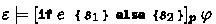
The formulae of probabilistic dynamic logic (pDL) are defined inductively as the smallest set generated by the following grammar:

$$\begin{aligned} \varphi \quad :\,\!:= \quad {{\textsf {ATF}}}~\mid ~\lnot \varphi ~\mid ~\varphi _1\wedge \varphi _2 ~\mid ~\forall l \cdot \varphi ~\mid ~[s]_{\boldsymbol{p}}\,\varphi \end{aligned}$$

(4)

where $\varphi$ ranges over pDL formulae, $l\! \in \! L$ over logical variables, s is a pGCL program with variables in $X$, and ${\boldsymbol{p}}$ is an expectation assigning values in [0, 1] to initial states of the program $s$. The logical operators $\rightarrow$, $\vee$ and $\exists$ are derived in terms of $\lnot$, $\wedge$ and $\forall$ as usual.

The last operator in Eq. (4) is known as the box-operator in dynamic logics, but now we give it a probabilistic interpretation along with the name “p-box.” Given a pGCL program s, we write $[s]_{\boldsymbol{p}}\,\varphi$ to express that the expectation that a formula $\varphi$ holds after successfully executing s is at least ${\boldsymbol{p}}$; i.e., the function ${\boldsymbol{p}}$ represents the expectation for $\varphi$ in the current state of $\mathcal {M}_s$ using ${[\![\varphi ]\!]}$ as the reward function (see Sect. 3). For the reader familiar with the CTL/PCTL terminology, the p-box formulae are path formulae, and all other formulae are state formulae.

We define semantics of well-formed formulae in pDL, so formulae with no free logical variables—all occurrences of logical variables are captured by a quantifier. The definition extends the standard satisfaction relation of dynamic logic [9] to the probabilistic case:

Definition 2

(Satisfaction of pDL  Formulae). Let $\varphi$ be a well-formed pDL formula, $\pi$ range over policies, $l \! \in \! L$, ${\boldsymbol{p}}: \textit{State} \rightarrow [0,1]$ be an expectation lower bound, and $\varepsilon$ be a valuation defined for all variables mentioned in $\varphi$. The satisfiability of a formula $\varphi$ in a model $\varepsilon$, denoted $\varepsilon \models \varphi$, is defined inductively as follows:

$$\begin{aligned}&\varepsilon \models \varphi&\text {iff}\quad&\varepsilon \models _{{\textsf {ATF}}}\varphi \quad \textrm{for}\quad \varphi \in {{\textsf {ATF}}}\\&\varepsilon \models \varphi _1\wedge \varphi _2&\textrm{iff}\quad&\varepsilon \models \varphi _1 \quad \textrm{and}\quad \varepsilon \models \varphi _2 \\&\varepsilon \models \lnot \varphi&\textrm{iff}\quad&\textrm{not}~ \varepsilon \models \varphi \\&\varepsilon \models \forall l \cdot \varphi&\textrm{iff}\quad&\varepsilon \models \varphi [ l := v ] ~\mathrm {for~each}~ v\in \textrm{dom}\,l \\&\varepsilon \models [s]_{\boldsymbol{p}}\varphi&\textrm{iff}\quad&{\boldsymbol{p}}(\varepsilon )\le \textbf{E}_{\varepsilon }{{[\![\varphi ]\!]}} ~\mathrm {where~the~expectation~is~taken~in}~\mathcal {M}_s \end{aligned}$$

For $\varphi \in {{\textsf {ATF}}}$, $\models _{{\textsf {ATF}}}$ can be used to check satisfaction just against the valuation of program variables since $\varphi$ is well-formed. In the case of universal quantification, the substitution replaces logical variables with constants. The last case (p-box) is implicitly recursive, since the characteristic function ${[\![\varphi ]\!]}$ refers to the satisfaction of $\varphi$ in the final states of $s$.

The satisfaction of a p-box formula $[s]_{\boldsymbol{p}}\,\varphi$ captures a lower bound on the probability of $\varphi$ holding after the program $s$. Consequently, pDL supports specification and reasoning about probabilistic reachability properties in almost surely terminating programs.

It is convenient to omit the valuation $\varepsilon$ from the satisfaction judgement, meaning that the judgement holds for all valuations (validity):

$$\begin{aligned} \models [s]_{{\boldsymbol{p}}}\, \varphi \quad \text {iff} \quad \varepsilon \models [s]_{{\boldsymbol{p}}}\, \varphi \quad \text {for all valuations } \varepsilon \end{aligned}$$

(5)

6 The P-Box Modality and Logical Connectives

We begin our investigation of pDL by exploring how the p-box operator interacts with different expectations and the other connectives of pDL.

In a proof system, weakening is useful to allow adjusting proven facts to a format of a syntactic proof rule. Since all operators of pDL, with the exception of p-box, behave like in first order logic, the usual qualitative weakening properties apply for these operators at the top-level. For instance, $\varphi _1 \wedge \varphi _2$ can be weakened to $\varphi _1$. These properties follow directly from Definition 2. The following proposition states the key properties for p-box:

Proposition 3

(Weakening). Let $\varepsilon$ stand for a valuation, ${\boldsymbol{p}}, {\boldsymbol{0}} \in \textit{State} \rightarrow [0, 1]$ be expectation lower bounds, s a pGCL program, and $\varphi \in {{\textsf {pDL}}}$. Then:

• 1. Universal lower bound: $\varepsilon \models [s]_{\boldsymbol{0}}\, \varphi$

• 2. Quantitative weakening: $\varepsilon \models [s]_{{\boldsymbol{p}}_1}\, \varphi$ then $\varepsilon \models [s]_{{\boldsymbol{p}}_2}\, \varphi \text { if } {\boldsymbol{p}}_2 \le {\boldsymbol{p}}_1$ everywhere

• 3. Weakening conjunctions: $\varepsilon \models [s]_{{\boldsymbol{p}}}\, (\varphi _1 \wedge \varphi _2)$ then $\varepsilon \models [s]_{{\boldsymbol{p}}}\, \varphi _i \text { ~for } i = 1, 2$

• 4. Qualitative weakening: $\varepsilon \models [s]_{{\boldsymbol{p}}}\, \varphi _1$ and $\models \varphi _1 \rightarrow \varphi _2$ then $\varepsilon \models [s]_{{\boldsymbol{p}}}\, \varphi _2$ .

The first point states that there is a limit to the usefulness of weakening the expectation: if you cannot guarantee that the lower bound is positive, then you do not have any information at all. A zero lower-bound would hold for any property. The second property is a probabilistic variant of weakening, which follows directly from the last case of Definition 2; the lower bound on an expectation can always be lowered. The last two properties are the probabilistic counterparts of weakening in standard (non-probabilistic) dynamic logic; the third property is syntactic for conjunction, the last one is general.

When building proofs with pDL, the other direction of reasoning seems more useful: we would like to be able to derive a conjunction from two independently concluded facts. For state formulae, this holds naturally, like in first-order logic. For p-box formulae, we would like to use the expectations ${\boldsymbol{p}}_i$ of two formulae $\varphi _i$ to draw conclusions about the expectation that their conjunction holds. It seems tempting to translate the intuitions from the Boolean lattice to real numbers, and to suggest that a minimum of the expectations for both formulae is a lower bound for their conjunction. To develop some intuition, let us first consider an incorrect proposal using the following counterexample:

Example 4

Consider the program , modeling a six-sided fair die:

$$\text{IMAGE}$$

Let ‘odd’ be an atomic formula stating that a value is odd, and ‘prime’ an atomic formula stating that it is prime. Since the die is fair, the expectations for each of these after are:

$$\text{IMAGE}$$

The minimum of the two expectations is a constant function which equals ${\boldsymbol{1/2}}$ everywhere, but the expectation bound in $[s]_{{\boldsymbol{p}}}(\text {odd} (x) \wedge \text {prime} (x))$ can be at most ${\boldsymbol{1/3}}$ since only two outcomes ($x\mapsto 3$ and $x\mapsto 5$) satisfy both predicates. Effectively, even if $\varepsilon \models [s]_{{\boldsymbol{p}}_1} \, \varphi _1$ and $\varepsilon \models [s]_{{\boldsymbol{p}}2} \, \varphi _2$ hold, we do not necessarily have $\varepsilon \models [s]_{\min ({\boldsymbol{p}}_1, {\boldsymbol{p}}_2)} \, \varphi _1 \wedge \varphi _2$. The reason is that the expectation bounds measure what is the lower bound on satisfaction of a property, but not where in the execution space this probability mass is placed. There is not enough information to see to what extent the two properties are overlapping.    $\square$

Similarly, ${\boldsymbol{p}}(\varepsilon ) = {\boldsymbol{p}}_1 (\varepsilon ) {\boldsymbol{p}}_2 (\varepsilon )$ is not a good candidate in Example 4, since it is only guaranteed to be a lower bound for a conjunction when $\varphi _i$ are independent events. Unless ${\boldsymbol{p}}_1 \! = \! {\boldsymbol{p}}_2 \! = \! {\boldsymbol{1}}$, combining proven facts with conjunction (or disjunction) weakens the expectation:

Theorem 5

Let $\varepsilon$ be a valuation, ${\boldsymbol{p}}, {\boldsymbol{p}}_1, {\boldsymbol{p}}_2 \in \textit{State} \rightarrow [0, 1]$ expectation lower bounds, s a pGCL program, and $\varphi _1, \varphi _2 \in {{\textsf {pDL}}}$. Then:

• 1. p-box conjunction: if $\varepsilon \models [s]_{{\boldsymbol{p}}_1}\, \varphi _1$ and $\varepsilon \models [s]_{{\boldsymbol{p}}_2}\, \varphi _2$, then $\varepsilon \models [s]_{{\boldsymbol{p}}}\, ( \varphi _1 \wedge \varphi _2 )$ where ${\boldsymbol{p}}= \max ( {\boldsymbol{p}}_1\! + \! {\boldsymbol{p}}_2 -1, 0 )$ everywhere.

• 2. p-box disjunction: if $\varepsilon \models [s]_{{\boldsymbol{p}}_1}\, \varphi _1$ or $\varepsilon \models [s]_{{\boldsymbol{p}}_2}\, \varphi _2$, then $\varepsilon \models [s]_{{\boldsymbol{p}}}\, ( \varphi _1 \vee \varphi _2 )$ where ${\boldsymbol{p}}= \min ({\boldsymbol{p}}_1, {\boldsymbol{p}}_2)$ everywhere.

Note the asymmetry between these cases: reasoning about conjunctions of low probability properties using Theorem 5.1 is inefficient, and quickly arrives at the lower bound expectation ${\boldsymbol{0}}$, which, as observed in Proposition 3, holds vacuously. If both properties have an expected probability lower than $1/2$, then pDL cannot really see (in a compositional manner) whether there is any chance that they can be satisfied simultaneously. In contrast, compositional reasoning about disjunctions makes sense both for low and high probability events. This is a consequence of using lower bounds on expectations. The bounds in Theorem 5 are consistent with prior work by Baier et al. on LTL verification of probabilistic systems [27].

The qualitative non-probabilistic specialization of Theorem 5.1 behaves reasonably: when $\varphi _1$ or $\varphi _2$ hold almost surely, then the theorem reduces to a familiar format:

$$\begin{aligned} \text {if } \varepsilon \models [s]_{{\boldsymbol{p}}} \varphi _1 \text { and } \varepsilon \models [s]_{{\boldsymbol{1}}} \varphi _2 \text { then } \varepsilon \models [s]_{{\boldsymbol{p}}} (\varphi _1 \wedge \varphi _2) \end{aligned}$$

(6)

Theorem 6

Let $\varepsilon$ be a valuation, ${\boldsymbol{p}} \in \textit{State} \!\rightarrow \! [0, 1]$ an expectation lower bound, $s$ a pGCL program, and $\varphi \in {{\textsf {pDL}}}$ a well-formed formula.

• 1. If $\varepsilon \models [s]_{{\boldsymbol{p}}}\, \forall l \cdot \varphi$  then  $\varepsilon \models \forall l \cdot [s]_{{\boldsymbol{p}}}\, \varphi$, but not the other way around in general.

• 2. If $\varepsilon \models \exists l \cdot [s]_{{\boldsymbol{p}}}\, \varphi \text { ~then~ } \varepsilon \models [s]_{{\boldsymbol{p}}}\, \exists l \cdot \varphi$ but not the other way around in general.

The essence of the above two properties lies in the fact that quantifiers in pDL only affect logical variables, programs cannot access logical variables, and we do not allow quantification over expectation variables.

In a deductive proof system, one works with abstract states, not just concrete states. A state abstraction can be introduced as a precondition, a pDL property that captures the essence of an abstraction, and is satisfied by all the abstracted states sharing the property. If an abstract property is a precondition for a proof, it is naturally introduced using implication. However, implication is unwieldy in an expectation calculus, so it is practical to be able to eliminate it in the proof machinery. The following theorem explains how a precondition can be folded into an expectation function:

Theorem 7

(Implication Elimination). Let $s$ be a pGCL program, $\varphi _i$ be pDL formulae, and ${\boldsymbol{p}}$ a lower-bound function for expectations. Then:

$$ \models \varphi _1 \rightarrow ([s]_{{\boldsymbol{p}}}\, \varphi _2) \quad \text {iff} \quad \models [s]_{{\boldsymbol{p}}\downarrow \varphi _1} \varphi _2 $$

Note that we use validity naturally when working with abstract states, as the state is replaced by the precondition in the formula.

Finally, negation in pDL is difficult to push over boxes. This is due to non-determinism and the lower bound semantics of expectations it enforces. A p-box property expresses a lower bound on probability of a post-condition holding after a program. Naturally, a negation of a p-box property will express an upper-bound on a property, but pDL has no upper-bound modality first-class. We return to this problem in Sect. 8, where we discuss reasoning about upper-bounds in non-deterministic and in purely probabilistic programs.

7 Expectations for Program Constructs

This section investigates how expectations are transformed by pGCL program constructs, as opposed to logical constructs discussed above. We begin by looking at the composite statements, which build the structure of the underlying MDP. The probabilistic choice introduces a small expectation update, consistent with an expectation of a Bernoulli variable (item 1). The demonic choice (item 2), requires that both sides provide the same guarantee, which is consistent with worst-case reasoning.

Theorem 8

(Expectation and Choices). Let $s_i$ be programs, $\varphi$ a PDL formula, ${\boldsymbol{p}}_i$ lower bound functions for expectations into [0, 1], and $\varepsilon$ a valuation of variables. Then:

• 1. If $\varepsilon \models [s_1]_{{\boldsymbol{p}}_1} \varphi$ and $\varepsilon \models [s_2]_{{\boldsymbol{p}}_2} \varphi$ then $\varepsilon \models [s_1 {\,}_{e}\!\oplus s_2]_{{\boldsymbol{p}}} \, \varphi$

  with ${\boldsymbol{p}}= \varepsilon (e){\boldsymbol{p}}_1 \! + \! ( 1 \! - \! \varepsilon (e)) {\boldsymbol{p}}_2$

• 2. $\varepsilon \models [s_1]_{{\boldsymbol{p}}} \, \varphi$ and $\varepsilon \models [s_2]_{{\boldsymbol{p}}} \, \varphi$ if and only if $\varepsilon \models [ s_1 \sqcap s_2 ]_{{\boldsymbol{p}}}\, \varphi$

Note that in the second case, demonic, we can always use weakening (Proposition 3.2) to equalize the left-hand-side expectation lower-bounds using a point-wise minimum, if the premises are established earlier for different lower bound functions.

Example 9

This example shows that a non-deterministic assignment is less informative than a probabilistic assignment. It shows that pDL can be used to make statements that compare programs directly in the formal system—one of its distinctive features in comparison with prior works (cf. Sect. 2). We check satisfaction of the following pDL formula for any expectation lower bound ${\boldsymbol{p}}$:

For simplicity, we use the logical variable p directly in the rightmost program (this can easily be encoded as an additional assumption equating a fresh logical variable to a program variable). For the proof, we first simplify the formula using equivalence rewrites:

In the last line above the left expectation is taken in MDP and the right one is taken in .

Now the property is a disjunction of three cases. If the first or second disjunct hold the formula holds vacuously (the assumptions in the statement are violated). We focus on the last case, when the first two disjuncts are violated (so the assumptions hold). We need to show that the last disjunct holds. We split the reasoning in two cases:

• 1. $\delta \le 0$: Consider the right expectation $\textbf{E}_{\varepsilon }({x \ge \delta })$. In the right program this expectation is equal to $1$ because the formula always holds (both possible values of $x$ are greater or equal to $\delta$). Consequently, any expectation lower bound ${\boldsymbol{p}}$ is correct for this formula: ${\boldsymbol{p}}(\varepsilon ) \le \textbf{E}_{\varepsilon }({x \ge \delta })$ in the right program.

• 2. $\delta > 0$: Consider the left expectation $\textbf{E}_{\varepsilon }({x \ge \delta })$. By Eq. (3) this expectation is equal to zero (the policy that chooses the left branch in the program violates the property as $x = 0 < \delta$). Since ${\boldsymbol{p}}(\varepsilon ) \le \textbf{E}_{\varepsilon }({x \ge \delta }) = 0$, it must be that ${\boldsymbol{p}}(\varepsilon ) = 0$ in the left program. By the universal lower bound property (Proposition 3.1), all properties hold after any program with the expectation lower bound ${\boldsymbol{p}}$, including the post-condition of the right program.    $\square$

For any program logic, it is essential that we can reason about composition of consecutive statements; allowing the post-condition of one to be used as a pre-condition for the other. The following theorem demonstrates that sequencing in pGCL corresponds to composition of expectations in the MDP domain. It uses implication elimination (Theorem 7) to compute a post-condition for a sequence of programs. Crucially, the new lower bound is computed using an expectation operation in the MDP of the first program, using the lower-bound of the second program as a reward function. Here, the expectation operation acts as a way to explore the program graph and accumulate values in final states.

Theorem 10

(Expectation and Sequencing). Let $s_i$ be pGCL programs, $\varphi _i$ be pDL formulae, $\varepsilon$ be a valuation, and ${\boldsymbol{p}}$ an expectation lower bound function.

$$\begin{aligned} \text { If }\models \varphi _1 \rightarrow ([s_2]_{{\boldsymbol{p}}} \, \varphi _2) \text { then } \varepsilon \models [s_1;s_2]_{_{\textbf{E}}{_{\langle \varepsilon ,s_1\rangle }({{\boldsymbol{p}}\downarrow \varphi _1})}} \, \varphi _2 , \end{aligned}$$

where the expectation $\textbf{E}_{\langle \varepsilon ,s_1\rangle }({{\boldsymbol{p}}\!\downarrow \!\varphi _1})$ is taken in $\mathcal {M}_{s_1}$ with ${\boldsymbol{p}}\!\downarrow \!\varphi _1$ as the reward function.

For a piece of intuition, note that the above theorem captures the basic step of a backwards reachability algorithm for MDPs, but expressed in pDL; it accumulates expectations backwards over $s_1$ from what is already known for $s_2$.

We now move to investigating how simple statements translate expectations:

Theorem 11

(Unfolding Simple Statements). Let $s$ be a pGCL program, $\varphi$ a pDL formula, ${\boldsymbol{p}}$ a function into $[0,1]$, a lower bound on expectations, and $\varepsilon$ a valuation. Then

• 1. iff $\varepsilon \models \varphi$

• 2. $\varepsilon \models [s]_{{\boldsymbol{p}}}\, \varphi$   iff  

• 3.   iff   $\varepsilon [x \mapsto \varepsilon (e)] \models [s]_{{\boldsymbol{p}}}\, \varphi$

The case of if-conditions below is rather classic (Theorem 12.3). For any given state, we can evaluate the head condition and inherit the expectation from the selected branch. For this to work we assume that the atomic formulae (${{\textsf {ATF}}}$) satisfaction semantics in pDL is consistent with the expression evaluation semantics in pGCL. The case of while loops is much more interesting—indeed a plethora of works have emerged recently on proposing sound reasoning rules for while loop invariants, post-conditions and termination (see Sect. 2). In this paper, we show the simplest possible reasoning rule for loops that performs a single unrolling, exactly along the operational semantics. Of course, we are confident that many other rules for reasoning about while loops (involving invariants, prefixes, or converging chains of probabilities) can also be proven sound in pDL—left as future work.

Theorem 12

(Unfolding Loops and Conditionals). Let $e$ be a program expression (also an atomic pDL formula over program variables in $X$), $\varphi$ be a pDL atomic formula, $s_i$ be pGCL programs, ${\boldsymbol{p}}$ an expectation lower bound function, and $\varepsilon$ a valuation. Then:

• 1. If $\varepsilon \models e \wedge [ s_1 ]_{{\boldsymbol{p}}}\, \varphi$ then

• 2. If $\varepsilon \models \lnot e \wedge [ s_2 ]_{{\boldsymbol{p}}}\, \varphi$ then

• 3. iff

8 Purely Probabilistic and Deterministic Programs

The main reason for the lower-bound expectation semantics in pDL (inherited from McIver & Morgan) is the presence of demonic choice in pGCL. With non-determinism in the language, calculating precise probabilities is not possible. However, this does not mean that pDL cannot be used to reason about upper-bounds. The following theorem explains:¹

Theorem 13

(Joni’s Theorem). For a policy $\pi$, property $\varphi$, program $s$, and state $\varepsilon$: if $\varepsilon \models [s]_{{\boldsymbol{p}}_1} \varphi$ and $\varepsilon \models [s]_{{\boldsymbol{p}}_2} \lnot \varphi$ then $\mathbb E_{ \pi , \varepsilon } {[\![\varphi ]\!]}\in [ p_1, 1-p_2 ]$.

The theorem means that for a purely probabilistic program derived by fixing a policy for a pGCL program s, the expected reward is bounded from below by the expectation of this reward in $s$, and from above by the expectation of its negation in $s$. The theorem follows directly from Eq. (3) and the negation case in Definition 2.

For deterministic programs, some surprising properties, follow from interaction of probability and logics. For instance, we can conclude a conjunction of expectations from an expectation of a disjunction.

Theorem 14

Let s be a purely probabilistic pGCL program (a program that does not use the demonic choice), let $\varepsilon$ stand for a valuation, ${\boldsymbol{p}} \in \textit{State} \rightarrow [0, 1]$ be an expectation function, and $\varphi _i \in {{\textsf {pDL}}}$ properties. Then if $\varepsilon \models [s]_{{\boldsymbol{p}}} \, ( \varphi _1 \vee \varphi _2 )$ then there exist ${\boldsymbol{p}}_1$, ${\boldsymbol{p}}_2$, ${\boldsymbol{p}}_1 + {\boldsymbol{p}}_2 \ge {\boldsymbol{p}}$ everywhere, such that $\varepsilon \models [s]_{{\boldsymbol{p}}_1}\, \varphi _1$ and $\varepsilon \models [s]_{{\boldsymbol{p}}_2}\, \varphi _2$.

Intuitively, the property holds, because each of the measure of the space of final states of the disjointed properties can be separated between the disjuncts. This separation would not be possible with non-determinism, as shown in the following counterexample.

Example 15

Consider the program . The following holds for any initial valuation $\varepsilon$:

This happens because disjunction is weakening and a weaker property is harder to avoid, here impossible to avoid, for an adversary minimizing an expectation satisfaction. However, at the same time: . Importantly, zero is the tightest expectation lower bound possible here.    $\square$

9 Program Analysis with pDL

In this section, we apply pDL to reason about two illustrative examples: the Monty Hall game (Sect. 9.1), and convergence of a Bernoulli random variable (Sect. 9.2).

9.1 Monty Hall Game

In this section, we use pDL to compute the probability of winning the Monty Hall game. In this game, a host presents 3 doors, one of which contains a prize and the others are empty, and a contestant must figure out the door behind which the prize is hidden. To this end, the host and contestant follow a peculiar sequence of steps. First, the location of the prize is non-deterministically selected by the host. Secondly, the contestant chooses a door. Then, the host opens an empty door from those that the contestant did not choose. Finally, the contestant is asked whether she would like to switch doors. We determine, using pDL, what option increases the chances of winning the prize (switching or not).

Listing 1.1 shows a pGCL program, , modeling the behavior of host and contestant. There are 4 variables in this program: (door containing the prize), (door selected by the contestant), (door opened by the host), (Boolean indicating whether the user switches in the last step). Note that the variable is undefined in the program. The value of encodes the strategy of the contestant, so its value will be part of a pDL specification that we study below. Line 1 models the hosts’s non-deterministic choice of the door for the prize. Line 2 models the door choice of the contestant (uniformly over the 3 doors). Lines 3–6 model the selection of the door to open, from the non-selected doors by the contestant. Lines 7–10 model whether the contestant switches door or not. For clarity and to reduce the size of the program, in lines 6 and 8, we use a shortcut to compute the door to open and to switch, respectively. Note that for $x,y \in \{0,1,2\}$ the expression $z = (2x-y)\;\textbf{mod}\;3$ simply returns $z \in \{0,1,2\}$ such that $z \not = x$ and $z\not =y$. Similarly, in line 4, the expressions $y=(x+1)\;\textbf{mod}\;3, z=(x+2)\;\textbf{mod}\;3$ ensure that $y\not =x$, $z\not =x$ and $y \not = z$. This shortcut computes the doors that the host may open when the contestant’s choice (line 2) is the door with the prize.

We use pDL to find out the probability of the contestant selecting the door with the prize. To this end, we check satisfaction of the following formula, and solve it for ${\boldsymbol{p}}$.

(7)

First, we show that ${\boldsymbol{p}}= \min ({\boldsymbol{p}}_0,{\boldsymbol{p}}_1,{\boldsymbol{p}}_2)$ where each ${\boldsymbol{p}}_i$ is the probability for the different locations of the prize. Formally, we use Theorem 8.2 (twice) as follows

For each ${\boldsymbol{p}}_i$, we compute the probability for each branch of the probabilistic choice. To this end, we use Theorem 8.1 as follows:

and apply it again for ${\boldsymbol{p}}_{i1}$ to resolve the inner probabilistic choice:

These steps show that ${\boldsymbol{p}}_i = 1/3\cdot {\boldsymbol{p}}_{i0} + 2/3\cdot 1/2\cdot {\boldsymbol{p}}_{i10} + 2/3\cdot 1/2\cdot {\boldsymbol{p}}_{i11}$ where ${\boldsymbol{p}}_{i0}$, ${\boldsymbol{p}}_{i10}$ and ${\boldsymbol{p}}_{i11}$ are the probabilities for the paths with $\textit{choice}$ equals to 0, 1 and 2, respectively.

Let us focus on the case ${\boldsymbol{p}}_1$. This is the case when the prize is behind door 1, $\varepsilon [\textit{prize} \mapsto 1]$. In what follows, we explore the three possible branches of the probabilistic choice. Consider the case where the user chooses door 1, i.e., $\varepsilon [\textit{choice} \mapsto 1]$ and

where and correspond to lines 4 and 6 in Listing 1.1, respectively. Since $\varepsilon \models \textit{prize} = \textit{choice}$ holds and by Theorem 12.1 we derive that

Note that ${\boldsymbol{p}}_{110}$ remains unchanged. Statement contains a non-deterministic choice, so we apply Theorem 8.2 to derive ${\boldsymbol{p}}_{110} = \min ({\boldsymbol{p}}_{1100},{\boldsymbol{p}}_{1101})$ where each ${\boldsymbol{p}}_{110i}$ correspond to the cases where $\varepsilon [\textit{open} \mapsto 2]$ and $\varepsilon [\textit{open} \mapsto 0]$, respectively. Since $\textit{switch} = \textit{true}$ both branches execute line 8, and the probabilities remain the same (Theorem 12.1). A simple calculation shows that after executing line 8 $\varepsilon \not \models (\textit{prize} = \textit{choice})$ for both cases. For instance, consider

By Theorem 11.3$\varepsilon [\textit{choice} \mapsto (2*1-0)\%3 = 2]$, which results in $\textit{prize} \not = \textit{choice}$. By the universal lower bound rule (Proposition 3.1) we derive ${\boldsymbol{p}}_{1100} = 0$. The same derivations show that ${\boldsymbol{p}}_{1101} = 0$, and, consequently, ${\boldsymbol{p}}_{110} = 0$.

The same reasoning shows that $\textit{prize}=\textit{choice}$ holds for the cases where $\textit{choice} \not =1$ in line 2, i.e., ${\boldsymbol{p}}_{i0}$ and ${\boldsymbol{p}}_{i11}$—we omit the details as they are analogous to the steps above. In these cases, by Theorem 11.1 we derive that ${\boldsymbol{p}}_{i0} = 1$ and ${\boldsymbol{p}}_{i11} = 1$. Recall that ${\boldsymbol{p}}_{110} = 0$ (see above), then we derive that ${\boldsymbol{p}}_1 = 1/3\cdot 1 \; + \; 2/3\cdot 1/2 \cdot 0 \; + \; 2/3\cdot 1/2\cdot 1$. Consequently, ${\boldsymbol{p}}_1 = 1/3 + 1/3 = 2/3$. Analogous reasoning shows that all ${\boldsymbol{p}}_i = 2/3$.

To summarize, the probability of choosing the door with the prize when switching is at most 2/3. In other words, we have proven that switching door maximizes the probability of winning the prize.

9.2 Convergence of a Bernoulli Random Variable

We use pDL to study the convergence of a program that estimates the expectation of a Bernoulli random variable. To this end, we compute the probability that an estimated expectation is above an error threshold $\delta > 0$. This type of analysis may be of practical value for verifying the implementation of estimators for statistical models.

Consider the following pGCL program for estimating the expected value of a Bernoulli random variable (Technically the program computes the number of successes out of $n$ trials, and we will put the estimation into the post-condition):

Intuitively, computes the average of n Bernoulli trials $X_i$ with mean $\mu$, i.e., $X = \sum _i X_i/n$. It is well-known that $\textrm{E}[X] = \mu$ (e.g., [28]). Each $X_i$ can be seen as a sample or measurement to estimate $\mu$. A common way to study convergence is to check the probability that the estimated mean X is within some distance $\delta > 0$ of $\mu$, i.e., $\Pr (|X-\mu | > \delta )$. In , a sample $X_i$ corresponds to the execution of the probabilistic choice ${\,}_{\mu \,}\!\oplus$ in line 3 of Listing 1.2. After running all loop iterations, variable c contains the sum of all the samples, i.e., $c = \sum _i X_i$. Thus, X is equivalent to c/n and the specification of convergence can be written as $\Pr (|c/n - \mu | > \delta )$. Note that this specification is independent of the implementation of the program. The same specification can be used for any program estimating $\mu$—by simply replacing X with the term estimating $\mu$ in the program.

In pDL, we can study the convergence of this estimator by checking

for some value of $\mu \in [0,1], \, \delta > 0$ and $n \in \mathbb {N}$. Note that, since the program contains no non-determinism, ${\boldsymbol{p}}= \Pr (|X-\mu | > \delta )$. We describe the reasoning to compute ${\boldsymbol{p}}$.

First, note that the while-loop in is bounded. Therefore, we can replace it with a sequence of n iterations of the loop body. Let $s_i$ denote the ith iteration of the loop (lines 3–4 in Listing 1.2). We omit for brevity the assignments in line 1 of Listing 1.2 and directly proceed with a state $\varepsilon [c \mapsto 0, i \mapsto 0]$. Consider the first iteration of the loop, i.e., $i=0$. By Theorem 12.3 we can derive

Assume $\varepsilon \models 0 < n$ holds, then by Theorem 12.1 we derive

By applying the above rules repeatedly we can rewrite as

with the added in the last iteration of the loop by Theorem 12.3 and 12.2.

Second, we compute the value of ${\boldsymbol{p}}$ for a possible path of . Consider the case when $c=0$ after executing the program. That is,

This only happens for the path where the probabilistic choice is resolved as for all loop iterations. Applying Theorem 10 we derive

Here $\textbf{E}_{\varepsilon }$ is computed over (cf. Theorem 10). For , this expectation is computed over the two paths resulting from the probabilistic choice in Listing 1.2, line 3. Since only the left branch satisfies $c=0$ and it is executed with probability $\mu$, then $\textbf{E}_{\varepsilon }{{\boldsymbol{p}}'} = \mu {\boldsymbol{p}}'$. Applying this argument for each iteration of the loop we derive that holds for ${\boldsymbol{p}}= \mu ^n$. Similarly, consider the case where $c=1$ after running all iterations of the loop, due to the first iteration resulting in and the rest . Then, we apply Theorem 10 as follows

In this case, $\textbf{E}_{\varepsilon }{{\boldsymbol{p}}'} = (1-\mu ) {\boldsymbol{p}}'$, as the probability of $c=1$ is $(1-\mu )$ (cf. Listing 1.2 line 3). Since, in this case, the remaining iterations of the loop result in , and from our reasoning above, we derive that ${\boldsymbol{p}}' = \mu ^{n-1}$. Hence, ${\boldsymbol{p}}= (1-\mu )\mu ^{n-1}$. In general, by repeatedly applying these properties, we can derive that the probability of a path is $\mu ^i(1-\mu )^j$ where i is the number loop iterations resulting in and j the number of loop iterations resulting in .

Fig. 3.

Convergence of Bernoulli random variable with $\mu =0.5$.

Now we return to our original problem . Recall from Definition 2 that ${\boldsymbol{p}}$ is the sum of the probabilities over all the paths that satisfy the post-condition. has $2^n$ paths (two branches per loop iteration). Therefore, we conclude that ${\boldsymbol{p}}= \sum _{i \in \varPhi } \mu ^{\textit{zeros(i)}}(1-\mu )^{\textit{ones(i)}}$ where $\textit{zeros}(\cdot ), \textit{ones}(\cdot )$ are functions returning the number of zeros and ones in the binary representation of the parameter, respectively, and $\varPhi = \{\,i \in 2^n \, \mid \, |\textit{ones}(i)/n - \mu | > \delta \,\}$ enumerates all paths in the program satisfying the post-condition. Note that the binary representation of $0,\ldots ,2^n$ conveniently captures each of the possible executions of .

The result above is useful to examine the convergence of . It allows us to evaluate the probability of convergence for increasing number of samples and different values of $\mu$ and $\delta$. As an example, Fig. 3 shows the results for $\mu =0.5$, $\delta \in \{0.1,0.2,0.4\}$ and up to $n=20$ iterations of the loop. The dotted and dashed lines in the figure show that with 20 iterations the probability of having an error $\delta >0.2$ is less than $5\%$. However, for an error $\delta > 0.1$ the probability increases to more than $20\%$.

10 Conclusion

This paper has proposed pDL, a specification language for probabilistic programs—the first dynamic logic for probabilistic programs written in pGCL. Like pGCL, pDL contains probabilistic and demonic choice. Unlike pGCL, it includes programs as first-order entities in specifications and allows forward reasoning capabilities as usual in dynamic logic. We have defined the model-theoretic semantics of pDL and shown basic properties of the newly introduced p-box modality. We demonstrated the reasoning capabilities on two well-known examples of probabilistic programs. In the future, we plan to develop a deductive proof system for pDL supported by tools for (semi-)automated reasoning about pGCL programs. Furthermore, the current definition of pDL gives no syntax to the expectations. Batz et al. propose a specification language for real-valued functions that is closed under the construction of weakest pre-expectations [20]; such a language could be used to express assertions for pGCL programs. It would be interesting to integrate these advances into pDL.

References

Kozen, D.: Semantics of probabilistic programs. In: Proceedings 20th Annual Symposium on Foundations of Computer Science, IEEE Computer Society, 101–114 (1979)
Hark, M., Kaminski, B.L., Giesl, J., Katoen, J.: Aiming low is harder: induction for lower bounds in probabilistic program verification. In: Proceedings of ACM Programming Language, 4(POPL), pp. 37:1–37:28 (2020)
Kaminski, B.L.: Advanced weakest precondition calculi for probabilistic programs. PhD thesis, RWTH Aachen University, Germany (2019)
Stein, D., Staton, S.: Compositional semantics for probabilistic programs with exact conditioning. In: Proceedings on 36th Annual ACM/IEEE Symposium on Logic in Computer Science (LICS 2021), pp. 1–13 IEEE (2021)
Smolka, S., Kumar, P., Foster, N., Kozen, D., Silva, A.: Cantor meets Scott: semantic foundations for probabilistic networks. In: Castagna, G., Gordon, A.D., (eds.) Proceedings of the 44th ACM SIGPLAN Symposium on Principles of Programming Languages (POPL 2017), pp. 557–571. ACM (2017)
Batz, K., et al.: Foundations for entailment checking in quantitative separation logic. In: Sergey, I. (ed.) ESOP 2022. LNCS, vol. 13240, pp. 57–84. Springer, Cham (2022). https://doi.org/10.1007/978-3-030-99336-8_3
McIver, A., Morgan, C.: Abstraction, Refinement And Proof For Probabilistic Systems. Monographs in Computer Science. Springer, Cham (2005)
Dijkstra, E.W.: A discipline of programming. Prentice-Hall (1976)
Harel, D., Kozen, D., Tiuryn, J.: Dynamic Logic. Foundations of Computing, MIT Press, Cambridge (2000)
Hansson, H., Jonsson, B.: A logic for reasoning about time and reliability. Formal Aspects Comput. 6(5), 512–535 (1994)
Puterman, M.L.: Markov Decision Processes. Wiley, Hoboken (2005)
Ahrendt, W., Beckert, B., Bubel, R., Hähnle, R., Schmitt, P.H., Ulbrich, M. (eds.): Deductive Software Verification - The KeY Book - From Theory to Practice. Lecture Notes in Computer Science, vol. 10001. Springer, Cham (2016)
de Gouw, S., Rot, J., de Boer, F.S., Bubel, R., Hähnle, R.: OpenJDK’s Java.utils.Collection.sort() is broken: The good, the bad and the worst case. In: Kroening, D., Pasareanu, C.S., (eds.) Proceedings of 27th International Conference on Computer Aided Verification (CAV 2015), Lecture Notes in Computer Science, vol. 9206, pp. 273–289 Springer, Cham (2015)
Pardo, R., Johnsen, E.B., Schaefer, I., Wąsowski, A.: A specification logic for programs in the probabilistic guarded command language (extended version). ArXiv: https://arxiv.org/abs/2205.04822 (2022)
Cousot, P., Monerau, M.: Probabilistic abstract interpretation. In: Seidl, H. (ed.) ESOP 2012. LNCS, vol. 7211, pp. 169–193. Springer, Heidelberg (2012). https://doi.org/10.1007/978-3-642-28869-2_9
Filieri, A., Pasareanu, C.S., Visser, W.: Reliability analysis in symbolic pathfinder. In: 35th International Conference on Software Engineering (ICSE 2013). IEEE Computer Society, pp. 622–631 (2013)
Kwiatkowska, M.Z., Norman, G., Parker, D.: The PRISM benchmark suite. In: Ninth International Conference on Quantitative Evaluation of Systems (QEST 2012). IEEE Computer Society, pp. 203–204 (2012)
Kozen, D.: A probabilistic PDL. J. Comput. Syst. Sci. 30(2), 162–178 (1985)
Feldman, Y.A., Harel, D.: A probabilistic dynamic logic. In: Proceedings of the 14th Annual ACM Symposium on Theory of Computing (STOC), pp. 181–195. ACM (1982)
Batz, K., Kaminski, B.L., Katoen, J., Matheja, C.: Relatively complete verification of probabilistic programs: an expressive language for expectation-based reasoning. Proc. ACM Program. Lang. 5(POPL), 1–30 (2021)
Hähnle, R.: Dijkstra’s legacy on program verification. In: Apt, K.R., Hoare, T., (eds.).: Edsger Wybe Dijkstra: His Life, Work, and Legacy. ACM / Morgan & Claypool, pp. 105–140 (2022)
Gretz, F., Katoen, J., McIver, A.: Operational versus weakest pre-expectation semantics for the probabilistic guarded command language. Perform. Eval. 73, 110–132 (2014)
McIver, A., Morgan, C., Kaminski, B.L., Katoen, J.: A new proof rule for almost-sure termination. Proc. ACM Program. Lang. 2(POPL), 33:1–33:28 (2018)
Batz, K., Kaminski, B.L., Katoen, J., Matheja, C., Noll, T.: Quantitative separation logic: a logic for reasoning about probabilistic pointer programs. Proc. ACM Program. Lang. 3(POPL), 34:1–34:29 (2019)
Kaminski, B.L., Katoen, J.-P., Matheja, C., Olmedo, F.: Weakest precondition reasoning for expected run–times of probabilistic programs. In: Thiemann, P. (ed.) ESOP 2016. LNCS, vol. 9632, pp. 364–389. Springer, Heidelberg (2016). https://doi.org/10.1007/978-3-662-49498-1_15
Aguirre, A., Barthe, G., Hsu, J., Kaminski, B.L., Katoen, J., Matheja, C.: A pre-expectation calculus for probabilistic sensitivity. Proc. ACM Program. Lang. 5(POPL), 1–28 (2021)
Baier, C., Kwiatkowska, M.Z., Norman, G.: Computing probability bounds for linear time formulas over concurrent probabilistic systems. Electron. Notes Theor. Comput. Sci. 22, 29 (1999)
Dekking, F.M., Kraaikamp, C., Lopuhaä, H.P., Meester, L.E.: A Modern Introduction to Probability and Statistics: Understanding Why and How. STS, Springer, London (2005). https://doi.org/10.1007/1-84628-168-7
Acknowledgments
This work was supported by the Research Council of Norway via SIRIUS (project no. 237898).
Author information
Authors and Affiliations
Corresponding author
Editor information
Editors and Affiliations
Rights and permissions
Copyright information
© 2022 The Author(s), under exclusive license to Springer Nature Switzerland AG
About this paper
Cite this paper
Pardo, R., Johnsen, E.B., Schaefer, I., Wąsowski, A. (2022). A Specification Logic for Programs in the Probabilistic Guarded Command Language. In: Seidl, H., Liu, Z., Pasareanu, C.S. (eds) Theoretical Aspects of Computing – ICTAC 2022. ICTAC 2022. Lecture Notes in Computer Science, vol 13572. Springer, Cham. https://doi.org/10.1007/978-3-031-17715-6_24
Download citation
DOI: https://doi.org/10.1007/978-3-031-17715-6_24
Published:
Publisher Name: Springer, Cham
Print ISBN: 978-3-031-17714-9
Online ISBN: 978-3-031-17715-6
eBook Packages: Computer ScienceComputer Science (R0)