Sobolev Spaces and Elliptic Boundary Value Problems

Abstract

In this course, we are interested to the resolution of elliptical equations with various types of boundary conditions: Dirichlet, Neumann or Fourier-Robin, Navier or Navier type conditions. We will study the existence, the uniqueness, and the regularity of the solutions. This regularity will depend, as we will see, on data of the problem and, in particular, of the regularity of the domain. For the sake of clarity and simplification, we will examine two model problems, one involving the Laplacian and the other the Stokes operator.

1 Sobolev Spaces, Inequalities, Dirichlet, and Neumann Problems for the Laplacian

1.1 Sobolev Spaces

Let us introduce the following Sobolev spaces: for any 1 < p < ∞

$$\displaystyle \begin{aligned}W^{m,p} (\Omega) = \left\{u \in \mathscr{D}^\prime (\Omega);\; \forall \, |\alpha| \leq m,\, D^\alpha u \in L^p (\Omega)\right\} \end{aligned}$$

and

$$\displaystyle \begin{aligned}W^{s,p} (\Omega) = \left\{u \in W^{m,p}(\Omega); \; \int_\Omega \int_\Omega \frac{\left| D^\alpha u(x) - D^\alpha u(y)\right|{}^p}{|x-y|{}^{N + \sigma p}} < \infty,\, \forall \, |\alpha| = m \right\}, \end{aligned}$$

where $m \in \mathbb {N}, s = m + \sigma , 0 < \sigma < 1$ and Ω is an open set of $\mathbb {R}^N.$ Equipped with the graph norm, they are Banach spaces.

When $\Omega = \mathbb {R}^N$, using the Fourier transform, we define for any real number s the space

$$\displaystyle \begin{aligned}H^s (\mathbb{R}^N) = \left\{u \in \mathscr{S}^\prime (\mathbb{R}^N); \int_{\mathbb{R}^N} (1 + |\xi|{}^2)^s \, |\hat{u}(\xi)|{}^2 \, d\xi < \infty \right\}, \end{aligned}$$

which is an Hilbert space for the norm:

$$\displaystyle \begin{aligned}\Vert u\Vert_{H^s(\mathbb{R}^N)} = \left(\int_{\mathbb{R}^N} (1+|\xi|{}^2)^{s}\vert\hat{u}\vert^2 dx\right)^{1/2}. \end{aligned}$$

By Plancherel’s theorem we prove that $W^{s,2}(\mathbb {R}^N) = H^s(\mathbb {R}^N)$ for all s ≥ 0 and this identity is algebraical and topological. So, in the case p = 2, we denote more simply the space W ^{s, 2}( Ω) by H ^s( Ω).

Definition 1.1

For s > 0 and 1 ≤ p < ∞, we denote

$$\displaystyle \begin{aligned}W_0^{s,p}(\Omega) = \overline{\mathscr{D}(\Omega)}^{\left\| \cdot \right\|{}_{W^{s,p}(\Omega)}}, \end{aligned}$$

and its topological dual space

$$\displaystyle \begin{aligned}W^{-s,p^\prime}(\Omega) = \left[W^{s,p}_0 (\Omega)\right]^\prime, \end{aligned}$$

where p ^′ is the conjugate of p: 1∕p + 1∕p ^′ = 1. For p = 2, we will write $H_0^{s}(\Omega )$ and H ^−s( Ω), respectively.

Proposition 1.2

Suppose $T \in \mathscr {D}^\prime (\Omega )$ . Then $T \in W^{-m,p^\prime } (\Omega )$ , with $m \in \mathbb {N}^*$ , if and only if

$$\displaystyle \begin{aligned}T = \displaystyle \sum_{|\alpha| \leq m} D^\alpha f_\alpha,\quad \mathrm{with}\quad f_\alpha \in L^{p^\prime}(\Omega). \end{aligned}$$

1.2 First Properties

It will be assumed from now on that Ω is a bounded open subset of $\mathbb {R}^N$ with a Lipschitz boundary.

Let us consider the following space

$$\displaystyle \begin{aligned}\mathscr{D}(\overline{\Omega}) = \left\{v_{|\Omega}; \; v \in \mathscr{D}(\mathbb{R}^N) \right\}. \end{aligned}$$

Theorem 1.3

• (i) The space $\mathscr {D}(\overline {\Omega })$ is dense in W ^{s, p}( Ω) for any s > 0 (even if Ω is unbounded).

• (ii) The space $\mathscr {D}(\mathbb {R}^N)$ is dense in $W^{s,p}(\mathbb {R}^N)$ for any $s \in \mathbb {R}$.

As consequence, we have the following property: for any s > 0

$$\displaystyle \begin{aligned}W^{s,p}_0 (\mathbb{R}^N) = W^{s,p}(\mathbb{R}^N)\quad \mathrm{and}\quad W^{-s,p^\prime} (\mathbb{R}^N ) = \left[W^{s,p}(\mathbb{R}^N)\right]^\prime. \end{aligned}$$

But in general, for any s > 0, we have $W^{s,p}_0 (\Omega ) \subsetneq W^{s,p} (\Omega ).$

Definition 1.4

For s > 0, we set

$$\displaystyle \begin{aligned}\widetilde{W}^{s,p} (\Omega) = \left\{u \in W^{s,p}(\Omega); \; \widetilde{u} \in W^{s,p}(\mathbb{R}^N) \right\}, \end{aligned}$$

where $\widetilde {u}$ is the extension by 0 of u outside of Ω.

The space $\widetilde {W}^{s,p}(\Omega )$ is a Banach space for the norm

$$\displaystyle \begin{aligned}\left\|u\right\|{}_{\widetilde{W}^{s,p}(\Omega)} = \left\| \widetilde{u}\right\|{}_{W^{s,p}(\mathbb{R}^N)}. \end{aligned}$$

It is easy to verify that for any nonnegative integer m

$$\displaystyle \begin{aligned} W^{m,p}_0 (\Omega) \hookrightarrow \widetilde{W}^{m,p}(\Omega) \end{aligned} $$

(1)

and for any $u \in W^{m,p}_0 (\Omega )$ we have

$$\displaystyle \begin{aligned} \left\|u\right\|{}_{\widetilde{W}^{m,p}(\Omega)} = \left\| u\right\|{}_{W^{m,p}(\Omega)}. \end{aligned} $$

(2)

When s = m + σ with 0 < σ < 1, we can show that

$$\displaystyle \begin{aligned} \left\|u\right\|{}_{\widetilde{W}^{s,p}(\Omega)} \simeq \left\|u\right\|{}_{W^{s,p}(\Omega)} + \displaystyle \sum_{|\alpha| = m} \left\| \frac{D^\alpha u}{\varrho^\sigma} \right\|{}_{L^p(\Omega)}, \end{aligned} $$

(3)

where ϱ(x) = d(x, Γ) and Γ = ∂ Ω.

Theorem 1.5

The space $\mathscr {D}(\Omega )$ is dense in $\widetilde {W}^{s,p}(\Omega )$ for all s > 0 (even if Ω is unbounded).

From (1), (2) and the definition of $W^{m,p}_0(\Omega )$, we deduce the following: for any $m \in \mathbb {N}^*,$

$$\displaystyle \begin{aligned} \widetilde{W}^{m,p}(\Omega) = W^{m,p}_0(\Omega). \end{aligned} $$

(4)

Theorem 1.6

For any 0 < s ≤ 1∕p, the space $\mathscr {D}(\Omega )$ is dense in W ^{s, p}( Ω), which means that

$$\displaystyle \begin{aligned} W^{s,p}_0(\Omega) = W^{s,p}(\Omega). \end{aligned} $$

(5)

Theorem 1.7

Let 0 < s ≤ 1 and $u \in W^{s,p}_0(\Omega ).$ Then

$$\displaystyle \begin{aligned}\frac{u}{\varrho^s} \in L^p (\Omega) \Longleftrightarrow s \neq 1/p \end{aligned}$$

and in this case

$$\displaystyle \begin{aligned}\left\|\frac{u}{\varrho^s}\right\|{}_{L^p(\Omega)} \leq C \, \vert u \vert_{W^{s,p}(\Omega)}, \end{aligned}$$

where the notation |⋅| denotes the semi-norm of W ^{s, p}( Ω).

The case s = 1 is known as Hardy’s inequality: for all $u \in W^{1,p}_0 (\Omega ),$

$$\displaystyle \begin{aligned}\left\|\frac{u}{\varrho}\right\|{}_{L^p(\Omega)} \leq C \, \left\|\nabla u\right\|{}_{L^p(\Omega)}. \end{aligned}$$

Using again a Hardy’s inequality, we prove the following result:

Theorem 1.8

Let s > 0 and $u \in W_0^{s,p}(\Omega ).$ Then for any |α|≤ s, we have

$$\displaystyle \begin{aligned} \frac{D^\alpha u}{\varrho^{s - |\alpha|}} \in L^p (\Omega) \Longleftrightarrow s - 1/p \notin \mathbb{N}. \end{aligned} $$

(6)

From (3) and (6), we deduce the following identity:

$$\displaystyle \begin{aligned} \widetilde{W}^{s,p}(\Omega) = W^{s,p}_0(\Omega) \end{aligned} $$

(7)

which holds for any s > 0 satisfying $s - 1/p \notin \mathbb {N}.$

Proposition 1.9

• (i) For any 1 ≤ j ≤ N and for any $s \in \mathbb {R}$ , the operator

  $$\displaystyle \begin{aligned} \frac{\partial }{\partial x_j} : W^{s,p}(\mathbb{R}^N) \longrightarrow W^{s-1,p}(\mathbb{R}^N) \end{aligned} $$

  (8)

  is continuous.

• (ii) However, if we replace $\mathbb {R}^N$ by Ω, Property (8) takes place unless s = 1∕p.

Sketch of the Proof of Point (ii)

1. Case :

s = m + σ, with $m\in \mathbb {N}^*$ and 0 ≤ σ < 1. Let u ∈ W ^{s, p}( Ω). By definition, we know that

$$\displaystyle \begin{aligned}u \in W^{m,p}(\Omega) \;\; \; \mbox{and} \; \; \; \int_\Omega \int_\Omega \frac{\left| D^\alpha u(x) - D^\alpha u(y)\right|{}^p}{|x-y|{}^{N + \sigma p}} <\infty, \quad \forall \, |\alpha| = m. \end{aligned}$$

So for any 1 ≤ j ≤ N

$$\displaystyle \begin{aligned}\frac{\partial u}{\partial x_j} \in W^{m-1,p}(\Omega) \quad \mbox{and} \quad \int_\Omega \int_\Omega \frac{\left| D^\alpha \frac{\partial u}{\partial x_j}(x) - D^\alpha \frac{\partial u}{\partial x_j}(y)\right|{}^p}{|x-y|{}^{N + \sigma p}} <\infty, \end{aligned}$$

for all |α| = m − 1. Consequently $\frac {\partial u}{\partial x_j} \in W^{s-1,p}(\Omega ).$

2. Case s ≤ 0.:

Let u ∈ W ^{s, p}( Ω). Since − s + 1 ≥ 1, for any $\varphi \in \mathscr {D}(\Omega )$, we get:

$$\displaystyle \begin{aligned}\begin{array}{ll} \left|\langle \frac{\partial u}{\partial x_j},\varphi\rangle_{ \mathscr{D}^\prime (\Omega) \times \mathscr{D}(\Omega)} \right| &= \left|- \langle u,\frac{\partial \varphi}{\partial x_j}\rangle_{\mathscr{D}^\prime (\Omega) \times \mathscr{D}(\Omega)} \right| \\ &\leq \left\| u\right\|{}_{W^{s,p}(\Omega)} \left\| \frac{\partial \varphi}{\partial x_j}\right\|{}_{W_0^{-s,p^\prime}(\Omega)}\\ &\leq \left\| u\right\|{}_{W^{s,p}(\Omega)} \left\| \varphi\right\|{}_{W_0^{-s +1,p^\prime}(\Omega)}. \end{array} \end{aligned}$$

We conclude by using the density of $\mathscr {D}(\Omega )$ in $W^{-s +1,p^\prime }_0(\Omega )$.

3. Case 0 < s < 1.:

Let u ∈ W ^{s, p}( Ω). Recall that Ω being Lipschitz open set, there exists an extension operator

$$\displaystyle \begin{aligned}\forall t \geq 0, \quad P : W^{t,p}(\Omega) \longrightarrow W^{t,p}(\mathbb{R}^N) \end{aligned}$$

which is linear, continuous, and satisfying

$$\displaystyle \begin{aligned}Pv_{|\Omega} = v, \quad \mbox{for any }\; v \in W^{t,p}(\Omega). \end{aligned}$$

As $Pu \in W^{s,p}(\mathbb {R}^N)$, we get $\frac {\partial Pu}{\partial x_j} \in W^{s-1,p} (\mathbb {R}^N).$ But

$$\displaystyle \begin{aligned}\left(\frac{\partial Pu}{\partial x_j} \right)_{|\Omega} = \frac{\partial u}{\partial x_j}, \end{aligned}$$

where $\frac {\partial u}{\partial x_j}$ is the restriction to Ω of the distribution $T = \frac {\partial Pu}{\partial x_j} \in W^{s-1,p}(\mathbb {R}^N)$. More precisely, we have:

$$\displaystyle \begin{aligned}\forall \, \varphi \in \mathscr{D}(\Omega), \quad \langle \frac{\partial u}{\partial x_j},\varphi \rangle_{\mathscr{D}^\prime(\Omega) \times \mathscr{D}(\Omega)} = \langle T, \widetilde{\varphi}\rangle_{\mathscr{D}^\prime(\mathbb{R}^N) \times \mathscr{D}(\mathbb{R}^N)}. \end{aligned}$$

That implies

$$\displaystyle \begin{aligned}\left| \langle \frac{\partial u}{\partial x_j},\varphi \rangle \right| \leq \left\|T\right\|{}_{W^{s-1,p}(\mathbb{R}^N)} \left\|\widetilde{\varphi}\right\|{}_{W^{1-s,p^\prime} (\mathbb{R}^N)} = \left\|T\right\|{}_{W^{s-1,p}(\mathbb{R}^N)} \left\|\varphi\right\|{}_{\widetilde{W}^{1-s,p^\prime} (\Omega)}. \end{aligned}$$

We have shown that $\frac {\partial u}{\partial x_j} \in \left [\widetilde {W}^{1-s,p^\prime }(\Omega )\right ]^\prime .$ But

$$\displaystyle \begin{aligned}\left[\widetilde{W}^{1-s,p^\prime}(\Omega)\right]^\prime = \left[W_0^{1-s,p^\prime}(\Omega)\right]^\prime \Longleftrightarrow 1-s \neq 1/p^\prime, \end{aligned}$$

i.e., s ≠ 1∕p. □

Remark 1

The above proof shows that

$$\displaystyle \begin{aligned}u \in W^{1/p,p}(\Omega) \Longrightarrow \frac{\partial u}{\partial x_j} \in \left[\widetilde{W}^{1/p^\prime,p^\prime}\right]^\prime. \end{aligned}$$

In particular,

$$\displaystyle \begin{aligned}u \in H^{1/2}(\Omega) \Longrightarrow \frac{\partial u}{\partial x_j}\in \left[\widetilde{H}^{1/2}(\Omega)\right]^\prime, \end{aligned}$$

where we remark also that

$$\displaystyle \begin{aligned}\widetilde{H}^{1/2}(\Omega) \hookrightarrow H^{1/2}(\Omega) = H^{1/2}_0 (\Omega). \end{aligned}$$

This embedding being dense, we get by duality

$$\displaystyle \begin{aligned}H^{-1/2} (\Omega) = \left[H^{1/2}_0 (\Omega)\right]^\prime \hookrightarrow \left[\widetilde{H}^{1/2}(\Omega)\right]^\prime . \end{aligned}$$

Corollary 1.10

Let s > 0. The following characterization holds:

$$\displaystyle \begin{aligned}u \in \widetilde{W}^{s,p}(\Omega) \Longleftrightarrow u \in W^{s,p}_0(\Omega) \quad \mathit{\mbox{and}} \quad \mathit{\mbox{for any}} \; |\alpha| = m, \; \; \frac{D^\alpha u}{\varrho^\sigma} \in L^p (\Omega), \end{aligned}$$

where $s = m + \sigma , m \in \mathbb {N}$ and 0 ≤ σ < 1.

1.3 Traces

Firstly, recall the following inclusions:

$$\displaystyle \begin{aligned}W^{s,p}(\mathbb{R}^N) \hookrightarrow \mathscr{C}^0 (\mathbb{R}^N) \quad \mbox{if} \quad s >\frac{N}{p}. \end{aligned}$$

So that if $u \in W^{s,p}(\mathbb {R}^N)$ with $s >\frac {N}{p}$, the restriction of u to the hyperplane x _N = 0 is well defined. But the continuity with respect to all variables is not necessary. It is enough to have the continuity with respect to the variable x _N. This is possible as soon as s > 1∕p.

Actually, we have the following result:

Theorem 1.11

• (i) Suppose that s − 1∕p = k + σ, with $k \in \mathbb {N}$ and 0 < σ < 1 (which implies, in particular, that $s- 1/p \notin \mathbb {N}$ ). Then the mapping

  

  where

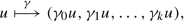
  $$\displaystyle \begin{aligned}\gamma_0 u (x) = u(x^\prime,0), x^\prime =(x_1,\ldots, x_{N-1}), \quad and\quad \gamma_j u (x^\prime) = \frac{\partial^j u}{\partial x_N^j} (x^\prime,0), \end{aligned}$$

  defined for $u \in \mathscr {D}(\mathbb {R}^N)$ , has a unique extension

  $$\displaystyle \begin{aligned}W^{s,p}(\mathbb{R}^n) \longrightarrow \displaystyle \prod_{j=0}^k W^{s-j-1/p,p}(\mathbb{R}^{N-1}) \end{aligned}$$

  which is continuous and where k is the integer part of s > 0.

• (ii) Moreover this operator has a right continuous inverse R:

  $$\displaystyle \begin{aligned}\left\{ \begin{array}{ll} \forall \, \boldsymbol{g} = (g_0,\ldots, g_k) \in \displaystyle \prod_{j=0}^k W^{s-j-1/p,p}(\mathbb{R}^{N-1}), \quad \gamma R \boldsymbol{g} = \boldsymbol{g} \\ \left\| R \boldsymbol{g} \right\|{}_{W^{s,p}(\mathbb{R}^N)} \leq C_N \, \displaystyle \sum_{j=0}^k \left\|g_j\right\|{}_{W^{s-j -1/p,p}(\mathbb{R}^{N-1})}. \end{array} \right. \end{aligned}$$

Remark 2

For p = 2, the above result can be proved using the Fourier transform.

This result can be extended to the case where Ω is a bounded open subset of $\mathbb {R}^{N}$, with a $\mathscr {C}^{k, 1}$ boundary (see the definition below).

Definition 1.12

Let Ω be an open subset of $\mathbb {R}^N$. We say that Ω is Lipschitz (respectively of class $\mathscr {C}^{k,1}, k \in \mathbb {N}^\star$) if for every x ∈ Γ, there exists a neighborhood V of x in $\mathbb {R}^N$ and orthonormal coordinates $\left \{y_1,\ldots ,y_N\right \}$ satisfying:

• (i) V is an hypercube

  $$\displaystyle \begin{aligned}V = \left\{(y_1,\ldots,y_N) \in \mathbb{R}^N; \; |y_j| <a_j, \; 1 \leq j \leq N \right\}, \end{aligned}$$

• (ii) there exists a function φ defined in

  $$\displaystyle \begin{aligned}V^\prime = \left\{ y^\prime\in \mathbb{R}^{N-1}; \; |y_j| < a_j, 1 \leq j \leq N-1 \right\}, \end{aligned}$$

  such that φ and φ ⁻¹ are Lipschitz (respectively, $\mathscr {C}^{k,1}$) and satisfying (Fig. 1)

  $$\displaystyle \begin{aligned}\forall \, y^\prime \in V^\prime , \quad \left|\varphi(y^\prime)\right| \leq \frac{1}{2} a_N \end{aligned}$$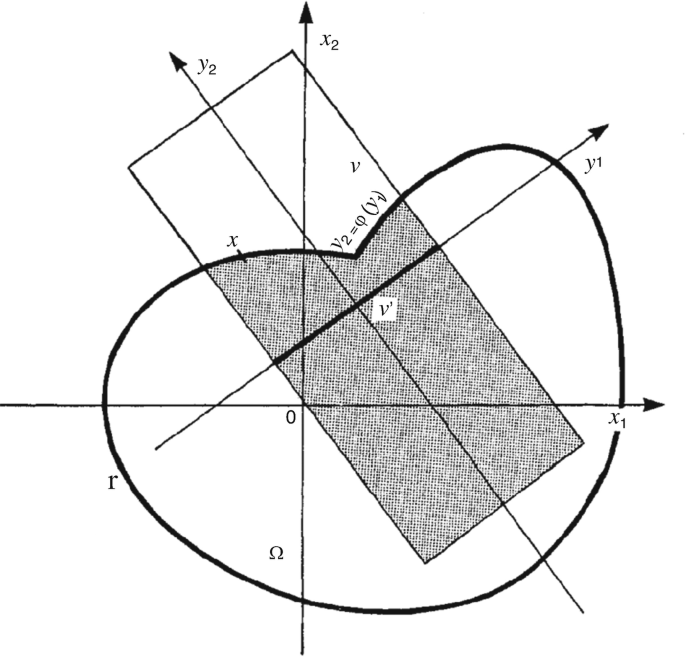

  

  Fig. 1

  $$\displaystyle \begin{aligned}\Omega \cap V = \left\{(y^\prime,y_N) \in V;\; y_N < \varphi (y^\prime) \right\} \end{aligned}$$
  $$\displaystyle \begin{aligned}\Gamma \cap V = \left\{(y^\prime,y_n) \in V; \; y_N = \varphi(y^\prime) \right\}. \end{aligned}$$

Let

$$\displaystyle \begin{aligned}\begin{array}{ll} \Phi : & V^\prime \longrightarrow \Gamma \cap V\\ & y^\prime \longmapsto (y^\prime,\varphi(y^\prime)). \end{array} \end{aligned}$$

Definition 1.13

Suppose that Ω is an open subset of $\mathbb {R}^N$ of class $\mathscr {C}^{k,1}$, with $k \in \mathbb {N}$ and let 0 < s ≤ k + 1. We introduce the following space

$$\displaystyle \begin{aligned}W^{s,p}(\Gamma) = \left\{u \in L^p(\Gamma);\; u\circ \Phi \in W^{s,p}(V^\prime \cap \Phi^{-1}(\Gamma \cap V)) \right\} \end{aligned}$$

for any (V, φ) verifying the previous definition.

Let (V _j, φ _j), 1 ≤ j ≤ J, be any atlas of Γ for which each pair (V _j, φ _j) satisfies the above definition. One possible Banach norm for W ^{s, p}( Γ) is given by:

$$\displaystyle \begin{aligned}\left\|u\right\|{}_{W^{s,p}(\Gamma)} = \displaystyle \sum_{j=1}^J \left\|u\circ \Phi_j\right\|{}_{W^{s,p}(V^\prime_j \cap \Phi_j^{-1} (\Gamma \cap V_j))} \end{aligned}$$

which is equivalent when 0 < s < 1 to the norm

$$\displaystyle \begin{aligned}\left(\left\|u\right\|{}^p_{L^p(\Gamma)} + \int_\Gamma \int_\Gamma \frac{\left|u(x) - u(y)\right|{}^p}{|x-y|{}^{N-1 + sp}} d\sigma_x d\sigma_y \right)^{1/p}. \end{aligned}$$

We are now in position to extend Theorem 1.11 to the case where $\mathbb {R}^{N-1}$ is replaced by an N − 1-dimensional manifold of $\mathbb {R}^N$, but which is sufficiently regular. This simply uses changes of variables.

If locally Γ is represented by the pair (V, φ) with φ and φ ⁻¹ Lipschitz, then a unit outward normal vector can be defined as follows:

$$\displaystyle \begin{aligned}\mbox{for}\; y^\prime \in V^\prime,\quad \boldsymbol{\nu}(y^\prime,\varphi(y^\prime)) = \frac{(-\nabla^\prime \varphi(y^\prime),1)}{\sqrt{1+ |\nabla^\prime \varphi (y^\prime)|{}^2}}. \end{aligned}$$

One can then extend this vector in all V by setting

$$\displaystyle \begin{aligned}\boldsymbol{\nu} (y^\prime,y_N) =\boldsymbol{\nu}(y^\prime,\varphi(y^\prime)), y \in V. \end{aligned}$$

As $\Gamma \subset \displaystyle \cup _{j=1}^J V_j$, we know that there exist functions $\mu _0, \mu _1,\ldots , \mu _J \in \mathscr {C}^\infty (\mathbb {R}^N)$ such that

• (i) for all j = 0, …, J, $0 \leq \mu _j \leq 1 \quad \mbox{and} \quad \displaystyle \sum _{j=1}^J \mu _j = 1$

• (ii) supp μ _j is compact and supp μ _j ⊂ V _j for any j ≥ 1 and supp μ ₀ ⊂ Ω.

This partition of unity then allows to extend ν in a neighborhood of $\overline {\Omega }$ as follows: $\boldsymbol {\nu } = \displaystyle \sum _{j=0}^J (\mu _j\boldsymbol {\nu }).$ It is then easy to verify that $\boldsymbol {\nu } \in L^\infty (\overline {\Omega })$ if Γ is Lipschitz and $\boldsymbol {\nu } \in \mathscr {C}^{k-1,1}(\overline {\Omega })$ if Γ is $\mathscr {C}^{k,1}$.

We are now ready to establish the following result:

Theorem 1.14 (Traces)

Let Ω be an open subset of $\mathbb {R}^N$ of class $\mathscr {C}^{k,1}$ , with $k \in \mathbb {N}$ . Let s > 0 satisfying s ≤ k + 1 and s − 1∕p = ℓ + σ with 0 < σ < 1 and $\ell \in \mathbb {N}.$ Then the mapping

defined for $\mathscr {C}^{k,1}$ has a unique continuous extension as an operator from W ^{s, p}( Ω) into $\displaystyle \prod _{j=0}^\ell W^{s-j - 1/p,p} (\Gamma )$ where

$$\displaystyle \begin{aligned}\gamma_1 u = \frac{\partial u}{\partial\boldsymbol{\nu}} = \nabla u \cdot \boldsymbol{\nu}, \quad \gamma_j u = \frac{\partial^j u}{\partial\boldsymbol{\nu}^j}. \end{aligned}$$

Moreover this operator has a right continuous inverse R (not depending of p).

Case Ω Lipschitz. Suppose 1∕p < s ≤ 1. We have the following properties:

• (i) If u ∈ W ^{s, p}( Ω), then u _{| Γ}∈ W ^{s−1∕p, p}( Γ).

• (ii) If g ∈ W ^{s−1∕p, p}( Γ), then there exists u ∈ W ^{s, p}( Ω) such that u = g on Γ and satisfying the estimate

  $$\displaystyle \begin{aligned}\left\|u\right\|{}_{W^{s,p}(\Omega)} \leq C \, \left\|g \right\|{}_{W^{s - 1/p,p}(\Gamma)}. \end{aligned}$$

Case Ω of class $\mathscr {C}^{1,1}$ .

• (i) Let u ∈ W ^{s, p}( Ω). If 1∕p < s ≤ 2, then u _{| Γ}∈ W ^1−1∕p( Γ). Moreover, for any g ∈ W ^{s−1∕p, p}( Γ), there exists u ∈ W ^{s, p}( Ω) such that u = g on Γ, with

  $$\displaystyle \begin{aligned}\left\|u\right\|{}_{W^{s,p}(\Omega)} \leq C \, \left\|g\right\|{}_{W^{s-1/p,p}(\Gamma)}. \end{aligned}$$

• (ii) Let u ∈ W ^{s, p}( Ω). If 1 + 1∕p < s ≤ 2, then $\frac {\partial u}{\partial \boldsymbol {\nu }} \in W^{s-1-1/p,p}(\Gamma ).$ Moreover, for any g ₀ ∈ W ^{s−1∕p, p}( Γ) and g ₁ ∈ W ^{s−1−1∕p, p}( Γ), there exists u ∈ W ^{s, p}( Ω) such that

  $$\displaystyle \begin{aligned}u = g_0 \quad \mbox{and} \quad \frac{\partial u}{\partial\boldsymbol{\nu}} = g_1 \quad \mbox{on} \; \Gamma \end{aligned}$$

  with

  $$\displaystyle \begin{aligned}\left\|u\right\|{}_{W^{s,p}(\Omega)} \leq C \, \left( \left\|g_0\right\|{}_{W^{s-1/p,p}(\Gamma)} + \left\|g_1\right\|{}_{W^{s-1-1/p,p}(\Gamma)}\right). \end{aligned}$$

Theorem 1.15

Suppose that Ω is an open subset of $\mathbb {R}^N$ of class $\mathscr {C}^{k,1}$ , with $k \in \mathbb {N}$ . Let s > 0 such that $s- 1/p \notin \mathbb {N}$ and s − 1∕p = ℓ + σ, where 0 < σ < 1 and ℓ ≥ 0 is an integer. Then we have the following characterization for s ≤ k + 1:

$$\displaystyle \begin{aligned}W^{s,p}_0(\Omega) = \left\{u \in W^{s,p}(\Omega); \gamma_0 u = \gamma_1 u = \ldots = \gamma_\ell u = 0 \right\}. \end{aligned}$$

1.4 Interpolation

We will consider here only the case of spaces H ^s( Ω), with Ω bounded open Lipschitz of $\mathbb {R}^N$.

Recall that for every s > 0 there exists a continuous linear operator:

$$\displaystyle \begin{aligned}P : H^s (\Omega) \longrightarrow H^s (\mathbb{R}^N) \end{aligned}$$

satisfying

$$\displaystyle \begin{aligned}\, \forall \, u \in H^s(\Omega), \quad Pu_{|\Omega} = u.\end{aligned} $$

Theorem 1.16

[Interpolation Inequality] Let s ₁, s ₂, s ₃ with 0 ≤ s ₁ < s ₂ < s ₃. Then

$$\displaystyle \begin{aligned}\forall \, \varepsilon > 0,\quad \left\|u\right\|{}_{W^{s_2,p}(\Omega)}\leq \varepsilon \left\|u\right\|{}_{W^{s_3,p}(\Omega)} + K\varepsilon^{- \frac{s_2-s_1}{s_3 - s_2}} \left\| u\right\|{}_{W^{s_1,p}(\Omega)},\end{aligned} $$

where K = K( Ω, s ₁, s ₂, s ₃, p).

The above inequality is a consequence of the compactness of the embedding of $W^{s_3,p}(\Omega )$ into $W^{s_2,p}(\Omega )$.

Recall now that we have different ways to define the Sobolev space H ^m( Ω), for $m \in \mathbb {N}$:

$$\displaystyle \begin{aligned} \begin{array}{ll} u \in H^m(\Omega) \iff \forall \, |\alpha| \leq m, \; D^\alpha u \in L^2(\Omega),\\ u \in H^m (\Omega)\iff u = U_{|\Omega} \; \mbox{with} \; U \in H^m (\mathbb{R}^N),\\ u \in H^m (\mathbb{R}^N) \iff u\in \mathscr{S}^\prime (\mathbb{R}^N) \quad \mathrm{and}\quad (1 + |\xi|{}^2)^{m/2} \hat{u} \in L^2(\mathbb{R}^N). \end{array} \end{aligned} $$

(9)

In the case of fractional Sobolev spaces H ^s( Ω), with $s = m + \sigma , m\in \mathbb {N}, 0 < \sigma < 1$, we have:

$$\displaystyle \begin{aligned} \begin{array}{ll} u \in H^s(\Omega) \iff u \in H^m(\Omega) \quad \mathrm{and}\quad \forall \, |\alpha| = m,\; \int_\Omega \int_\Omega \frac{\left|D^\alpha u(x) - D^\alpha u(y)\right|}{|x-y|{}^{N + 2 \sigma}} < \infty\\ u \in H^s (\Omega) \iff u = U_{|\Omega} \;\quad \mathrm{with} \quad U \in H^s (\mathbb{R}^N), \\ u \in H^s (\mathbb{R}^N) \iff u\in \mathscr{S}^\prime (\mathbb{R}^N) \quad \mathrm{and}\quad (1 + |\xi|{}^2)^{s/2} \hat{u} \in L^2(\mathbb{R}^N). \end{array} \end{aligned} $$

(10)

We can also get this space by interpolation:

$$\displaystyle \begin{aligned}H^s(\Omega) = \left[H^m(\Omega), L^2(\Omega)\right]_{\mu}, \, 0 <\mu < 1 \quad (1-\mu) m = s\end{aligned} $$

and more generally we have for any 0 < μ < 1

$$\displaystyle \begin{aligned}\left[H^{s_1}(\Omega), H^{s_2}(\Omega)\right]_{\mu} = H^{(1-\mu)s_1 + \mu s_2} (\Omega).\end{aligned} $$

Concerning the interpolation of spaces $H^m_0(\Omega )$, we have:

$$\displaystyle \begin{aligned}\left[H^{s_1}_0(\Omega), H^{s_2}_0(\Omega)\right]_{\mu} = H_0^{(1-\mu)s_1 + \mu s_2} (\Omega)\quad \mbox{ if }\quad (1-\mu) s_1 + \mu s_2\notin \frac{1}{2} + \mathbb{N}\end{aligned} $$

and

$$\displaystyle \begin{aligned}\left[H_0^{s_1}(\Omega), H_0^{s_2}(\Omega)\right]_{\mu} = \widetilde{H}^{(1-\mu)s_1 + \mu s_2} (\Omega)\quad \mathrm{otherwise}, \end{aligned}$$

with equivalent norms.

1.5 Transposition

Let V and H be two Hilbert spaces on $\mathbb {R}$ and $A \in \mathscr {L} (V,H)$. For every fixed g ∈ H ^′, we consider the following mapping

$$\displaystyle \begin{aligned}\begin{array}{ll} V & \longrightarrow \mathbb{R} \\ x & \longmapsto \langle g,Ax\rangle_{H^\prime \times H} \end{array}\end{aligned} $$

which defines a linear and continuous form on V that we denote by ^t Ag:

$$\displaystyle \begin{aligned}\langle ^t A g, x\rangle_{V^\prime \times V} = \langle g,Ax\rangle_{H^\prime \times H}. \end{aligned}$$

Remark 3

If A : V →H is an isomorphism, then we can define the transpose of A ⁻¹ and we easily verify that

$$\displaystyle \begin{aligned}^t{A^{-1}} = \left({}^t A\right)^{-1} \quad \mbox{and} \quad ^t A : H^\prime \longrightarrow V^\prime \; \mbox{is an isomorphism}.\end{aligned} $$

1.6 Inequalities

They are fundamental tools in the study of partial differential equations:

• (i) Poincaré’s Inequality. Let Ω be an open space bounded in at least one direction. Then there exists a constant C ≥ 0, depending on the diameter of Ω such that

  $$\displaystyle \begin{aligned}\forall \, u \in W^{1,p}_0 (\Omega),\quad \left\|u\right\|{}_{L^p(\Omega)} \leq C \, \left\|\nabla u\right\|{}_{L^p(\Omega)}.\end{aligned} $$

• (ii) Poincaré-Wirtinger’s Inequality. Let Ω be a Lipschitz bounded domain of $\mathbb {R}^N$. Then there exists a constant C( Ω) ≥ 0 such that

  $$\displaystyle \begin{aligned}\forall \, u \in W^{1,p}(\Omega),\quad \displaystyle \inf_{K \in \mathbb{R}} \left\|u + K\right\|{}_{L^p(\Omega)} \leq C(\Omega) \, \left\|\nabla u \right\|{}_{L^p(\Omega)}. \end{aligned}$$

• (iii) Hardy’s Inequality. Let Ω be a Lipschitz bounded open subset of $\mathbb {R}^N$. Then there exists a constant C( Ω) ≥ 0 such that

  $$\displaystyle \begin{aligned}\forall \, u \in W^{1,p}_0 (\Omega), \quad \left\|\frac{u}{\varrho}\right\|{}_{L^p(\Omega)} \leq C(\Omega) \, \left\|\nabla u \right\|{}_{L^p(\Omega)}. \end{aligned}$$

• (iv) Calderòn–Zygmund’s Inequality.

  $$\displaystyle \begin{aligned}\forall \, u \in \mathscr{D}(\Omega), \quad \left\|\frac{\partial^2 u}{\partial x_i \partial x_j}\right\|{}_{L^p(\Omega)} \leq C(\Omega) \, \left\|\Delta u \right\|{}_{L^p(\Omega)}. \end{aligned}$$

1.7 Weak Solutions

Consider the following problems:

$$\displaystyle \begin{aligned}(P_D) \quad - \Delta u = f \quad \mbox{in} \; \Omega \quad \quad \mathrm{and}\quad u = g \quad \mbox{on} \; \Gamma \end{aligned}$$

and

$$\displaystyle \begin{aligned}(P_N) \quad - \Delta u = f \quad \mbox{in} \; \Omega \quad \quad \mathrm{and}\quad \frac{\partial u}{\partial\boldsymbol{\nu}} = h \quad \mbox{on} \; \Gamma , \end{aligned}$$

where Ω is a Lipschitz bounded domain of $\mathbb {R}^N$, f, g, and h are given.

Theorem 1.17

Given any f ∈ H ⁻¹( Ω) and any g ∈ H ^1∕2( Γ), there exists a unique solution u ∈ H ¹( Ω) to Problem (P _D). Moreover

$$\displaystyle \begin{aligned}\left\|u\right\|{}_{H^1(\Omega)} \leq C(\Omega) \, \left(\left\|f\right\|{}_{H^{-1}(\Omega)} + \left\|g\right\|{}_{H^{1/2}(\Gamma)}\right). \end{aligned}$$

Proof

Using Theorem 1.14, there exists u _g ∈ H ¹( Ω) such that

$$\displaystyle \begin{aligned}u_g = g \quad \mbox{on} \; \Gamma \quad \mathrm{with} \quad \left\|u_g\right\|{}_{H^1(\Omega)} \leq C(\Omega) \, \left\|g \right\|{}_{H^{1/2}(\Gamma)}. \end{aligned}$$

Setting

$$\displaystyle \begin{aligned}f_g = - \Delta u_g = - \mathrm{div}\, \nabla u_g \in H^{-1}(\Omega), \end{aligned}$$

the problem becomes: Find $v\in H^1_0(\Omega )$ solution of

$$\displaystyle \begin{aligned}(P^0_D) \quad - \Delta v = f - f_g \quad \mbox{in} \; \Omega \quad \quad \mathrm{and}\quad v = 0 \quad \mbox{on} \; \Gamma . \end{aligned}$$

This last problem is equivalent to the following variational formulation:

$$\displaystyle \begin{aligned}(FV)_D \, \left\{ \begin{array}{ll} \mbox{Find} \; v \in H^1_0(\Omega) \; \mbox{such that} \\ \forall \, \varphi \in H^1_0(\Omega), \quad \displaystyle \int_\Omega \nabla v \cdot \nabla \varphi dx = \langle f- f_g, \varphi \rangle_{{H^{-1}(\Omega} \times H^1_0(\Omega)}. \end{array} \right. \end{aligned}$$

Applying Lax–Milgram Lemma or Riesz Theorem, we prove the existence of a unique solution $v \in H^1_0(\Omega )$ satisfying (FV )_D.

Note that the bilinear form

$$\displaystyle \begin{aligned}a(v,\varphi) = \int_\Omega \nabla v \cdot \nabla \varphi dx \end{aligned}$$

is continuous on $H^1_0(\Omega ) \times H^1_0(\Omega )$ and coercive on $H^1_0(\Omega )$ thanks to Poincaré’s inequality. In addition, this form allows to define a scalar product on Hilbert’s space $H^1_0(\Omega )$. □

Remark 4

• (i) If Ω is of class $\mathscr {C}^{1}$, f ∈ W ^{−1, p}( Ω) and g ∈ W ^{1−1∕p, p}( Γ) with 1 < p < ∞, then there exists a unique solution u ∈ W ^{1, p}( Ω) to (P _D).

• (ii) When Ω is only Lipschitz, this regularity result holds for p ∈ ]2 − ε ^′, 2 + ε[ where ε and ε ^′ > 0 are depending on Ω and 2 − ε ^′ and 2 + ε are conjugate.

Concerning the Neumann problem, the approach is a bit more complicated. Indeed, if we are looking for a solution u ∈ H ¹( Ω) only, the boundary condition on the normal derivative does not make sense, since the functions of L ²( Ω) do not have any trace at the boundary. Here, in fact, if one set v = ∇u we have

$$\displaystyle \begin{aligned}\frac{\partial u}{\partial\boldsymbol{\nu}} = \boldsymbol{v} \cdot \boldsymbol{\nu} \; \mbox{on} \; \Gamma. \end{aligned}$$

Definition 1.18

$$\displaystyle \begin{aligned}H(\mathrm{div};\, \Omega) = \left\{ \boldsymbol{v} \in L^2(\Omega); \; \mathrm{div}\, \boldsymbol{v} \in L^2(\Omega) \right\}. \end{aligned}$$

It is a Hilbert space for the scalar product

$$\displaystyle \begin{aligned}(( \boldsymbol{v},\boldsymbol{w}))_{H(\mathrm{div};\, \Omega)} = \int_\Omega \boldsymbol{v} \cdot \boldsymbol{w} dx + \int_\Omega (\mathrm{div}\, \boldsymbol{v}) (\mathrm{div}\, \boldsymbol{w}) dx. \end{aligned}$$

Proposition 1.19

• (i) The space $\mathscr {D}(\overline {\Omega })$ is dense in H(div;  Ω).

• (ii) The linear mapping

  $$\displaystyle \begin{aligned}\boldsymbol{v} \longmapsto \boldsymbol{v}\cdot \boldsymbol{\nu}, \end{aligned}$$

  defined on $\mathscr {D}(\overline {\Omega })^N,$ can be uniquely extended into a linear mapping of H(div; Ω) in $H^{-1/2}(\Gamma ):= \left [H^{1/2}(\Gamma )\right ]^\prime$.

• (iii) In addition, we have the following Green’s formula (or Stokes’ formula):

  $$\displaystyle \begin{aligned}\forall \varphi \in H^1(\Omega),\; \forall \boldsymbol{v}\in H(\mathrm{div}; \, \Omega),\quad \int_\Omega \boldsymbol{v} \cdot \nabla \varphi \, dx + \int_\Omega \varphi \, \mathrm{div}\, \boldsymbol{v} \, dx = \langle \boldsymbol{v}\cdot\boldsymbol{\nu},\varphi \rangle_{\Gamma} \end{aligned}$$

  where 〈⋅, ⋅〉_Γ denotes the duality brackets H ^−1∕2( Γ) × H ^1∕2( Γ).

Corollary 1.20

Let u ∈ H ¹( Ω) be such that Δu ∈ L ²( Ω). Then $\frac {\partial u}{\partial \boldsymbol {\nu }} \in H^{-1/2} (\Gamma ).$ Moreover for any φ ∈ H ¹( Ω), we have the following Green formula:

$$\displaystyle \begin{aligned}\int_\Omega \varphi \Delta u \, dx + \int_\Omega \nabla u \cdot \nabla \varphi \, dx = \langle \frac{\partial u}{\partial\boldsymbol{\nu}}, \varphi \rangle_\Gamma. \end{aligned}$$

Proof

It suffices to apply Proposition 1.19 by setting v = ∇u. □

As a Consequence we can show that for any f ∈ L ²( Ω) and for any g ∈ H ^−1∕2( Γ), the problems

$$\displaystyle \begin{aligned}(P_N) \, \left\{ \begin{array}{ll} \mbox{Find} \; u \in H^1(\Omega)\; \mbox{such that} \\ -\Delta u = f \quad \mbox{in} \; \Omega, \\ \frac{\partial u}{\partial\boldsymbol{\nu}} = g \quad \mbox{on} \; \Gamma \end{array} \right. \end{aligned}$$

and

$$\displaystyle \begin{aligned}(Q_N) \, \left\{ \begin{array}{ll} \mbox{Find} \; u \in H^1(\Omega) \; \mbox{such that} \\ \forall \, \varphi \in H^1(\Omega),\quad \displaystyle \int_\Omega \nabla u \cdot \nabla \varphi \, dx = \int_\Omega f \varphi \, dx + \langle g, \varphi \rangle_{\Gamma} \end{array} \right. \end{aligned}$$

are equivalent, so that any solution of one is a solution of the other.

Remark 5

• (i) The open Ω being bounded, the constant functions belong to H ¹( Ω). So that if u is a solution of (Q _N), taking φ = 1, the data f and g must satisfy the (necessary) compatibility condition:

  $$\displaystyle \begin{aligned}\int_\Omega f \, dx + \langle g,1\rangle_\Gamma = 0. \end{aligned}$$

• (ii) The implication (P _N)⇒(Q _N) results from Corollary 1.20. The reverse implication also uses Green’s formula and the surjectivity of the trace operator of H ¹( Ω) into H ^1∕2( Γ).

Theorem 1.21

Let Ω be a bounded, connected, and Lipschitzian open of $\mathbb {R}^N,$ with N ≥ 2. Let f ∈ L ²( Ω), g ∈ H ^−1∕2( Γ) satisfying the compatibility condition

$$\displaystyle \begin{aligned}\int_\Omega f \, dx + \langle g,1\rangle_\Gamma = 0. \end{aligned}$$

Then Problem (P _N) has a solution H ¹( Ω), unique to an additive constant, verifying the estimate:

$$\displaystyle \begin{aligned}\left\|\nabla u\right\|{}_{L^2(\Omega)} \leq C(\Omega) \, \left(\left\|f \right\|{}_{L^2(\Omega)} + \left\|g\right\|{}_{H^{-1/2}(\Gamma)} \right). \end{aligned}$$

Proof

According to Poincaré-Wirtinger’s inequality, we have

$$\displaystyle \begin{aligned}\displaystyle \inf_{K \in \mathbb{R}} \left\|u + K \right\|{}_{H^1(\Omega)} \leq C(\Omega) \, \left\|\nabla u \right\|{}_{L^2(\Omega)}. \end{aligned}$$

So that the bilinear form

$$\displaystyle \begin{aligned}a(u,\varphi) = \int_\Omega \nabla u \cdot\nabla \varphi \, dx \end{aligned}$$

is coercive on the quotient space $V = H^1(\Omega ) /_{ \displaystyle {\mathbb {R}}}$. It is then sufficient to apply Lax–Milgram on the Hilbert space V . □

Remark 6

• (i) We could have chosen as space V the space $H^1(\Omega ) \cap L^2_0(\Omega )$ where

  $$\displaystyle \begin{aligned}L^2_0(\Omega) = \left\{v \in L^2(\Omega); \int_\Omega v\, dx = 0 \right\}, \end{aligned}$$

  which is a Hilbert space and then use the inequality:

  $$\displaystyle \begin{aligned}\forall \, v \in H^1(\Omega) \cap L^2_0(\Omega), \quad \left\|v\right\|{}_{H^1(\Omega)} \leq C \, \left\| \nabla v\right\|{}_{L^2(\Omega)}. \end{aligned}$$

• (ii) We could have taken f in a space larger than L ²( Ω). More precisely if $f \in L^{(2^*)^\prime }(\Omega )$, where (2^∗)^′ is the conjugate of 2^∗ defined by

  $$\displaystyle \begin{aligned}\frac{1}{2^*} = \left\{ \begin{array}{ll} \frac{1}{2} - \frac{1}{N} \quad \mbox{if} \; N \geq 3 \\ \varepsilon > 0 \quad \mbox{arbitrary if} \;N =2, \end{array} \right. \end{aligned}$$

  i.e., $(2^*)^\prime = \frac {2N}{N + 2}$ if N ≥ 3 and (2^∗)^′ > 1 if N = 2.

• (iii) In L ^p-theory, we have existence results in W ^{1, p}( Ω) when Ω is $\mathscr {C}^{1}$ and 1 < p < ∞ or when Ω is $\mathscr {C}^{0,1}$ and 2 − ε ^′ < p < 2 + ε.

In the same spirit, we can consider the case of Fourier-Robin boundary condition:

$$\displaystyle \begin{aligned}(P_{FR}) \left\{ \begin{array}{ll} \mbox{Find} \; u \in H^1(\Omega) \\ - \Delta u = f \quad \mbox{in}\; \Omega, \\ \frac{\partial u}{\partial\boldsymbol{\nu}} + \alpha u = g \quad \mbox{on } \; \Gamma, \end{array} \right. \end{aligned}$$

where α is a positive function defined on Γ, which can be formulated in an equivalent way by:

$$\displaystyle \begin{aligned}(Q_{FR}) \left\{ \begin{array}{ll} \mbox{Find} \; u \in H^1(\Omega) \; \mbox{such that} \\ \forall \, \varphi \in H^1(\Omega), \quad \displaystyle \int_\Omega \nabla u \cdot \nabla \varphi \, dx + \int_\Gamma \alpha u \varphi \, dx = \int_\Omega f \varphi \, dx + \langle g,\varphi \rangle_\Gamma. \end{array} \right. \end{aligned}$$

1.8 Strong Solutions

Theorem 1.22

Let Ω be a bounded open of class $\mathscr {C}^{1,1}$ of $\mathbb {R}^N$ . Let f ∈ L ²( Ω) and g ∈ H ^∕2( Γ). Then the solution u given by Theorem 1.17 belongs to H ²( Ω) and verifies the estimate:

$$\displaystyle \begin{aligned}\left\|u\right\|{}_{H^2(\Omega)} \leq C(\Omega) \, \left( \left\|f\right\|{}_{L^2( \Omega)} + \left\|g\right\|{}_{H^{3/2}(\Gamma)} \right). \end{aligned}$$

Proof

Firstly, we note that

$$\displaystyle \begin{aligned}L^2(\Omega) \hookrightarrow H^{-1}(\Omega) \quad \mbox{and} \quad H^{3/2}(\Gamma) \hookrightarrow H^{1/2}(\Gamma) \end{aligned}$$

so that the problem (P _D) has a unique solution u ∈ H ¹( Ω).

We shift the data g ∈ H ^3∕2( Γ) by u _g ∈ H ²( Ω) and we set again u = v + u _g, so that v ∈ H ¹( Ω) vérifies:

$$\displaystyle \begin{aligned}\left\{ \begin{array}{ll} - \Delta v = f + \Delta u_g \in L^2(\Omega), \\ v = 0 \quad \mbox{on} \; \Gamma. \end{array} \right. \end{aligned}$$

So, we need to show that v ∈ H ²( Ω). One of the methods to establish this regularity consists in using the technique of the differential quotients.

The complete proof being long and tedious, we will admit it. □

Remark 7

We can also establish the existence of solutions in W ^{2, p}( Ω) when the data f and g verify:

$$\displaystyle \begin{aligned}f \in L^p(\Omega)\quad \mathrm{and} \quad g \in W^{2 - 1/p,p}(\Gamma) \end{aligned}$$

and the domain Ω is of class $\mathscr {C}^{1,1}$.

1.9 Very Weak Solutions

We assume here that Ω is a bounded open of class $\mathscr {C}^{1,1}$ and we are interested in the homogeneous problem

$$\displaystyle \begin{aligned}(P^H_{D}) \left\{ \begin{array}{ll} \mbox{Find} \; u \in L^2(\Omega) \\ - \Delta u = 0 \quad \mbox{in}\; \Omega, \\ u = g \quad \mbox{on } \; \Gamma, \end{array} \right. \end{aligned}$$

where g ∈ H ^−1∕2( Γ).

Remark 8

As the function u belongs “only” to L ²( Ω), the boundary condition u = g on Γ has a priori no sense. But we will see that in fact, we can make sense of the trace of a harmonic function in L ²( Ω) and (we can in fact weaken this last hypothesis).

Lemma 1.23

• (i) The space $\mathscr {D}(\overline {\Omega })$ is dense in the space

  $$\displaystyle \begin{aligned}E(\Omega;\Delta) = \left\{v \in L^2(\Omega);\; \Delta v \in L^2(\Omega) \right\}. \end{aligned}$$

• (ii) The mapping v↦v _{| Γ} defined on $\mathscr {D}(\overline {\Omega })$ can be uniquely extended into a continuous linear mapping of E( Ω; Δ) into H ^−1∕2( Γ).

• (iii) In addition, we have the following Green’s formula:

  $$\displaystyle \begin{aligned}\left\{ \begin{array}{ll} \forall \, v \in E(\Omega;\Delta),\quad \forall \, \varphi \in H^2(\Omega) \cap H^1_0(\Omega) \\ \displaystyle \int_\Omega v \Delta \varphi \, dx - \int_\Omega \varphi \Delta v\, dx = \langle v, \frac{\partial \varphi}{\partial\boldsymbol{\nu}} \rangle_{H^{-1/2}(\Gamma) \times H^{1/2}(\Gamma)}. \end{array} \right. \end{aligned}$$

Proof

• (i) The idea is to use the Hahn–Banach theorem. So let $\ell \in \left [E(\Omega ;\Delta )\right ]^\prime$ vanishing on $\mathscr {D}(\overline {\Omega })$ and show that it cancels on E( Ω; Δ).

  We know that there exist (f, g) ∈ L ²( Ω) × L ²( Ω) such that

  $$\displaystyle \begin{aligned}\forall \, v \in E(\Omega;\Delta), \quad \langle \ell,v\rangle = \int_\Omega f v \, dx + \int_\Omega g \Delta v \, dx. \end{aligned}$$

  Let $\widetilde {f}$ and $\widetilde {g}$ the extensions by 0 outside of Ω of f and g, respectively. Then, for any $v\in \mathscr {D}(\mathbb {R}^N)$

  $$\displaystyle \begin{aligned}\langle \ell,\, v_{\vert\Omega} \rangle = \int_\Omega fv \, dx + \int_\Omega g \Delta v \, dx = \int_{\mathbb{R}^N} \widetilde{f} v \, dx + \int_{\mathbb{R}^N} \widetilde{g} \Delta v \, dx, \end{aligned}$$

  i.e.,

  $$\displaystyle \begin{aligned}\Delta \widetilde{g} = - \widetilde{f} \; \mbox{in} \; \mathbb{R}^N. \end{aligned}$$

  As $\widetilde {g} \in L^2(\mathbb {R}^N)$ and $\Delta \widetilde {g} \in L^2(\mathbb {R}^N),$ then $\widetilde {g} \in H^2(\mathbb {R}^N)$. Therefore, g ∈ H ²( Ω). The extension $\widetilde {g}$, by 0 outside of Ω, belongs to $H^2(\mathbb {R}^N)$. We know then that $g \in H^2_0(\Omega )$. By definition, there exists a sequence (g _k)_k of functions of $\mathscr {D}(\Omega )$ such that g _k→g in H ²( Ω).

  Finally, let v ∈ E( Ω; Δ). So,

  $$\displaystyle \begin{aligned}\langle \ell,v \rangle = \displaystyle\lim_{k \Longrightarrow \infty} \left[ \int_\Omega - v \Delta v_k \, dx + \int_\Omega g_k \Delta v \, dx \right] = \displaystyle \lim_{k \Longrightarrow \infty} 0 = 0. \end{aligned}$$

• (ii) Let $v \in \mathscr {D}(\overline {\Omega })$ fixed and $\varphi \in H^2(\Omega ) \cap H^1_0 (\Omega )$. Then

  $$\displaystyle \begin{aligned}\int_\Omega v \Delta \varphi \, dx - \int_\Omega \varphi \Delta v \, dx = \int_\Gamma v \frac{\partial \varphi }{\partial\boldsymbol{\nu}}. \end{aligned}$$

  Now let μ ∈ H ^1∕2( Γ). According to the trace theorem and since Ω is of class $\mathscr {C}^{1,1}$, there exists φ ∈ H ²( Ω) verifying

  $$\displaystyle \begin{aligned}\left\{ \begin{array}{ll} \varphi = 0 \quad \mbox{and} \quad \frac{\partial \varphi}{\partial\boldsymbol{\nu}} = \mu \quad \mbox{on} \; \Gamma, \\ \left\|\varphi\right\|{}_{H^2(\Omega)} \leq C \, \left\|\mu\right\|{}_{H^{1/2}(\Gamma)}. \end{array} \right. \end{aligned}$$

  Thus, using the Cauchy–Schwarz inequality

  $$\displaystyle \begin{aligned}\left|\langle v,\mu\rangle_{H^{-1/2}(\Gamma) \times H^{1/2}(\Gamma)} \right| = \left| \int_\Gamma v \mu \right| = \left|\int_\Gamma v \frac{\partial \varphi}{\partial\boldsymbol{\nu}}\right| \end{aligned}$$
  $$\displaystyle \begin{aligned}\leq C(\Omega) \, \left( \left\|v\right\|{}^2_{L^2(\Omega)} + \left\|\Delta v \right\|{}_{L^2(\Omega)}^2 \right)^{1/2} \, \left\|\varphi\right\|{}_{H^2(\Omega)} \end{aligned}$$
  $$\displaystyle \begin{aligned}\leq C(\Omega) \left\|v\right\|{}_{E(\Omega;\Delta)} \left\|\mu\right\|{}_{H^{1/2}(\Gamma)}. \end{aligned}$$

  This shows that the linear mapping

  $$\displaystyle \begin{aligned}\begin{array}{ll} \mathscr{D}(\overline{\Omega}) & \longrightarrow H^{-1/2}(\Gamma) \\ \; \; \; \; v & \longmapsto v_{|\Gamma} \end{array} \end{aligned}$$

  is continuous when $\mathscr {D}(\overline {\Omega })$ is equipped with the norm of E( Ω; Δ). We finish the proof by using the density of $\mathscr {D}(\overline {\Omega })$ in E( Ω; Δ).

• (iii) Immediate.

□

Theorem 1.24

Let Ω be a bounded open of class $\mathscr {C}^{1,1}$ of $\mathbb {R}^N$ and let g ∈ H ^−1∕2( Γ). Then, the problem $(P_D^0)$ has a unique solution u ∈ L ²( Ω) verifying the estimate

$$\displaystyle \begin{aligned}\left\|u\right\|{}_{L^2(\Omega)} \leq C(\Omega) \, \left\|g\right\|{}_{H^{-1/2}(\Gamma)}. \end{aligned}$$

Proof

From Green’s formula above, it is easy to see that u ∈ L ²( Ω) is a solution of the problem $(P_D^0)$ if and only if

$$\displaystyle \begin{aligned} \forall \, \varphi \in H^2(\Omega) \cap H^1_0(\Omega), \quad \displaystyle \int_\Omega u \Delta \varphi \, dx = \langle g,\frac{\partial \varphi}{\partial\boldsymbol{\nu}} \rangle_\Gamma. \end{aligned} $$

(11)

Indeed, let u ∈ L ²( Ω) be a solution of $(P_D^0)$. Green’s formula implies that (11) takes place.

Conversely, let u ∈ L ²( Ω) be a solution of (11). Then, for all $\varphi \in \mathscr {D}(\Omega )$, we have

$$\displaystyle \begin{aligned}0 = \int_\Omega u \Delta \varphi \, dx = \langle \Delta u, \varphi\rangle_{\mathscr{D}^\prime (\Omega) \times \mathscr{D}(\Omega)}, \end{aligned}$$

i.e.,

$$\displaystyle \begin{aligned} \Delta u = 0 \quad \mbox{in} \; \Omega. \end{aligned} $$

(12)

Let now $\varphi \in H^2(\Omega ) \cap H^1_0(\Omega ).$ From (12) and Green’s formula above, we deduce successively that:

$$\displaystyle \begin{aligned}0 =\displaystyle \int_\Omega \varphi \Delta u \, dx = \int_\Omega u \Delta \varphi\, dx - \langle u,\frac{\partial \varphi}{\partial\boldsymbol{\nu}} \rangle_\Gamma \end{aligned}$$

then

$$\displaystyle \begin{aligned}\langle u,\frac{\partial \varphi}{\partial\boldsymbol{\nu}}\rangle_\Gamma = \langle g,\frac{\partial \varphi}{\partial\boldsymbol{\nu}}\rangle_\Gamma. \end{aligned}$$

From the surjectivity of the trace mapping $v \mapsto (v_{\vert \Gamma }, \frac {\partial v}{\partial \boldsymbol {\nu }})$ from H ²( Ω) into H ^3∕2( Γ) × H ^1∕2( Γ) we know that

$$\displaystyle \begin{aligned}\forall \mu \in H^{1/2}(\Gamma), \quad \langle u,\mu \rangle_\Gamma = \langle g,\mu \rangle_\Gamma, \end{aligned}$$

i.e., u = g in H ^−1∕2( Γ). □

Remark 9

A similar result can be established for the Neumann problem $(P_N^0)$ with boundary data h in H ^−3∕2( Γ) and satisfying the compatibility condition 〈h, 1〉_Γ = 0.

1.10 Solutions in H ^s( Ω), with 0 < s < 2

We have established in the previous paragraphs the existence of solutions in H ¹( Ω), H ²( Ω), and L ²( Ω) under generally optimal assumptions (except for the Neumann problem).

We will now consider the case of solutions in H ^s( Ω) with 0 < s < 2 and s ≠ 1. The main ingredient is to use interpolation (complex here).

Theorem 1.25

Let Ω be a bounded open of class $\mathscr {C}^{1,1}$.

• (i) Suppose that $\frac {1}{2} <s < 2.$ Then the operators

  $$\displaystyle \begin{aligned} \begin{array}{rl} & \Delta : H^s(\Omega) \cap H^1_0(\Omega) \longrightarrow H^{s-2}(\Omega) = \left[H_0^{2-s}(\Omega)\right]^\prime\quad \mathrm{if}\ \; 1 < s < 2 \; \mathrm{and}\; s \neq \frac{3}{2},\\ &\Delta : H^{3/2}_0(\Omega) \longrightarrow \left[H_{00}^{1/2}(\Omega)\right]^\prime, \\ & \Delta : H^{2-s}_0(\Omega) \longrightarrow H^{-s}(\Omega) = \left[H_0^{s}(\Omega)\right]^\prime \quad \mathrm{if}\ \; 1 < s < \frac{3}{2}, \end{array} \end{aligned} $$

  (13)

  are isomorphisms.

• (ii) For any g ∈ H ^s( Γ), with $-\frac {1}{2} < s < \frac {3}{2}$ , Problem $(P_D^H)$ has a unique solution $u \in H^{s + \frac {1}{2}} (\Omega )$.

Remark 10

What happens if Ω is only Lipschitz? For what values of s can we have u ∈ H ^s( Ω)?

2 The Stokes Problem with Various Boundary Conditions

We are interested here in the study of the Stokes problem:

$$\displaystyle \begin{aligned}(S) \, \left\{ \begin{array}{ll} \mbox{Find} \; (\boldsymbol{u}, \pi) \quad \mbox{satisfying} \\ - \Delta \boldsymbol{u} + \nabla \pi = \boldsymbol{f}\quad \mbox{in} \; \Omega, \\ \mathrm{div} \, \boldsymbol{u} = 0 \quad \mbox{in} \; \Omega, \end{array} \right. \end{aligned}$$

with one of the following boundary conditions on Γ:

• (i) u = 0 (Dirichlet boundary condition)

• (ii) u ⋅ν = 0 and curl u ×ν = 0 (Navier type boundary condition)

• (iii) $\boldsymbol {u} \cdot \boldsymbol {\nu } = 0 \; \mbox{and} \; (\mathbb {D}\boldsymbol {u})\boldsymbol {\nu } + \alpha \boldsymbol {u}_\tau = \mathbf {0} \; (\mbox{Navier boundary condition})$

• (iv) u ×ν = 0 and π = π ₀ (pressure boundary condition).

Here u denotes the velocity field, π the pressure field, Ω a connected bounded open set we assume at least Lipschitz.

Recall that

$$\displaystyle \begin{aligned}\mathrm{div}\ \, \boldsymbol{u} = \nabla \cdot \boldsymbol{u}, \quad \mathbf{curl}\, \boldsymbol{u} = \nabla \times \boldsymbol{u}\quad \mathrm{and}\quad \mathbb{D}\boldsymbol{u} = \frac{1}{2} \left( \nabla \boldsymbol{u} + (\nabla \boldsymbol{u})^T\right). \end{aligned}$$

The notation u _τ denotes the tangential component of u: u _τ = u − (u ⋅ν)ν. Finally f and α are given on Ω and Γ, respectively.

Remark 11

• (i) We limit ourselves here, with the exception of pressure, to the case of homogeneous boundary conditions.

• (ii) If the boundary of Ω is flat (like a cube, for example, or half space), the above boundary conditions are more easily written. When $\Omega = \mathbb {R}_+^3$, the Navier type boundary condition is equivalent to:

  $$\displaystyle \begin{aligned}u_3 = 0 \quad \mbox{and} \quad \frac{\partial u_1}{\partial x_3} = \frac{\partial u_2}{\partial x_3} = 0 \end{aligned}$$

  and that of Navier at:

  $$\displaystyle \begin{aligned}u_3 = 0 \quad \mbox{and} \quad \frac{\partial u_1}{\partial x_3} - \alpha u_1 = \frac{\partial u_2}{\partial x_3} - \alpha u_2 = 0. \end{aligned}$$

2.1 The Problem (S) with Dirichlet Boundary Condition

As for the Laplace equation with the Dirichlet boundary condition, we will assume

$$\displaystyle \begin{aligned}\boldsymbol{f}\in H^{-1}(\Omega)^3 \end{aligned}$$

and so look for $\boldsymbol {u} \in H^1_0(\Omega )^3$ verifying (S). Here we have in addition the constraint

$$\displaystyle \begin{aligned}\mathrm{div}\, \boldsymbol{u} = 0 \quad \mbox{in} \; \Omega \end{aligned}$$

and the Lagrange multiplier π. First of all, as π must verify

$$\displaystyle \begin{aligned}\nabla \pi = \boldsymbol{f}+ \Delta \boldsymbol{u} \in H^{-1}(\Omega)^3 \end{aligned}$$

it is, therefore, reasonable to look for π in L ²( Ω). Moreover, it is easy to verify that such π satisfies:

$$\displaystyle \begin{aligned}\forall \, \boldsymbol{v} \in H^1_0(\Omega)^3,\quad \langle \nabla \pi,\boldsymbol{v} \rangle_{H^{-1}(\Omega) \times H^1_0(\Omega)} = - \int_\Omega \pi \, \mathrm{div}\, \boldsymbol{v} \, dx. \end{aligned}$$

The space

$$\displaystyle \begin{aligned}V = \left\{\boldsymbol{v} \in H^1_0(\Omega)^3; \; \mathrm{div}\, \boldsymbol{v} = 0 \; \mbox{in} \; \Omega \right\} \end{aligned}$$

being a subspace of $H^1_0(\Omega )^3$ is, therefore, a Hilbert space. Moreover

$$\displaystyle \begin{aligned}\forall \, \boldsymbol{v} \in V, \quad \langle \nabla \pi,\boldsymbol{v} \rangle_{H^{-1}(\Omega) \times H^1_0(\Omega)} = 0. \end{aligned}$$

We are now able to propose a variational formulation of Problem (S):

$$\displaystyle \begin{aligned}(P_D^0) \, \left\{ \begin{array}{ll} \mbox{Find} \; \boldsymbol{u} \in V \; \mbox{such that} \\ \displaystyle \forall \, \boldsymbol{v} \in V,\quad \int_\Omega \nabla \boldsymbol{u} : \nabla \boldsymbol{v} \, dx = \langle \boldsymbol{f},\boldsymbol{v} \rangle_{H^{-1}(\Omega) \times H^1_0(\Omega)}, \end{array} \right. \end{aligned}$$

where we note that the pressure π has “disappeared.”

Lemma 2.1

The problem

$$\displaystyle \begin{aligned}(S_D^0) \, \left\{ \begin{array}{ll} \mathit{\mbox{Find}} \; (\boldsymbol{u}, \pi) \in H^1_0(\Omega)^3 \times L^2(\Omega)\\ - \Delta \boldsymbol{u} + \nabla \pi = \boldsymbol{f}\quad \mathit{\mbox{in}} \; \Omega, \\ \mathrm{div} \, \boldsymbol{u} = 0 \quad \mathit{\mbox{in}} \; \Omega \end{array} \right. \end{aligned}$$

is equivalent to the problem $(P_D^0)$.

Proof

The implication $(S_D^0) \Longrightarrow (P_D^0)$ is immediate. Conversely, let u be a solution of $(P_D^0)$. Then, in particular,

$$\displaystyle \begin{aligned}\forall \, \boldsymbol{v} \in \mathscr{D}(\Omega)^3 \quad \mbox{such that} \quad \mathrm{div}\, \boldsymbol{v} = 0 \quad \mbox{in} \; \Omega, \end{aligned}$$

we have

$$\displaystyle \begin{aligned} \langle - \Delta \boldsymbol{u} - \boldsymbol{f}, \boldsymbol{v} \rangle_{\mathscr{D}^\prime(\Omega)^3 \times \mathscr{D}(\Omega)^3} = 0. \end{aligned} $$

(14)

As − Δu −f ∈ H ⁻¹( Ω)³ and the space

$$\displaystyle \begin{aligned}\mathcal{V}(\Omega) = \left\{\boldsymbol{v} \in \mathscr{D}(\Omega)^3; \mathrm{div}\, \boldsymbol{v} = 0 \ \mbox{in} \; \Omega \right\} \end{aligned}$$

is dense in the space V , then the relation (14) takes place for all v. Then we know that there exists π ∈ L ²( Ω), unique up to an additive constant, because Ω is connected, such that

$$\displaystyle \begin{aligned}- \Delta \boldsymbol{u} - \boldsymbol{f}= \nabla(-\pi) \quad \mbox{in} \; \Omega \end{aligned}$$

(this result is called “De Rham’s version of the theorem” in H ⁻¹( Ω)^N). And finally, as u ∈ V , then

$$\displaystyle \begin{aligned}\mathrm{div}\, \boldsymbol{u} = 0 \; \mbox{in} \; \Omega \quad \mbox{and} \quad \boldsymbol{u} = \mathbf{0} \quad \mbox{on} \; \Gamma. \end{aligned}$$

This ends the proof of the lemma. □

Theorem 2.2

For any f ∈ H ⁻¹( Ω)³, the Stokes problem $(P_D^0)$ has a unique solution u ∈ V vérifying further

$$\displaystyle \begin{aligned}\left\|\boldsymbol{u}\right\|{}_{H^1(\Omega)^3} \leq C(\Omega) \, \left\|\boldsymbol{f}\, \right\|{}_{H^{-1}(\Omega)^3}. \end{aligned}$$

Proof

Simply apply Lax–Milgram theorem. □

Remark 12

The theory is well known for everything that concerns the regularity of solutions when the data are:

• solutions in W ^{1, p}( Ω)³ × L ^p( Ω)

• solutions in W ^{2, p}( Ω)³ × L ^p( Ω)

with 1 < p < ∞.

In particular, if f ∈ L ²( Ω)³ and Ω is of class $\mathscr {C}^{1,1}$, then u ∈ H ²( Ω)³ and π ∈ H ¹( Ω).

2.2 The Stokes Problem with Navier Type Boundary Condition

Here we are still interested in Stokes’ problem, but with the following boundary condition:

$$\displaystyle \begin{aligned}\boldsymbol{u} \cdot\boldsymbol{\nu} = 0 \quad \mbox{and} \quad \mathbf{curl}\, \boldsymbol{u} \times\boldsymbol{\nu} = \mathbf{0} \;\mbox{on} \; \Gamma. \end{aligned}$$

In order to take into account this condition at the boundary, it is important to write the Laplacian operator in the form:

$$\displaystyle \begin{aligned}- \Delta = \mathbf{curl}\, \mathbf{curl}\, - \nabla \, \mathrm{div}. \end{aligned}$$

On the other hand, if we study the existence of weak solutions u in H ¹( Ω)³, it will be necessary to give a meaning to the condition at the boundary

$$\displaystyle \begin{aligned}\mathbf{curl}\, \boldsymbol{u} \times \boldsymbol{\nu} = \mathbf{0} \quad \mbox{on} \; \Gamma. \end{aligned}$$

Recall the following Green formulas:

• (i) If v ∈ L ²( Ω)³ and curl v ∈ L ²( Ω)³, then v ×ν ∈ H ^−1∕2( Γ)³ and

  $$\displaystyle \begin{aligned}\forall \, \boldsymbol{\varphi} \in H^1(\Omega)^3, \quad \int_\Omega \boldsymbol{v} \cdot \mathbf{curl}\, \boldsymbol{\varphi} \, dx - \int_\Omega \boldsymbol{\varphi} \cdot \mathbf{curl}\, \boldsymbol{v} \, dx = \langle \boldsymbol{v} \times\boldsymbol{\nu}, \boldsymbol{\varphi} \rangle_\Gamma, \end{aligned}$$

  where 〈⋅, ⋅〉_Γ denotes the duality brackets H ^−1∕2( Γ) × H ^1∕2( Γ).

• (ii) If v ∈ L ²( Ω)³ and div v ∈ L ²( Ω), then v ⋅ν ∈ H ^−1∕2( Γ) and

  $$\displaystyle \begin{aligned}\forall \, \varphi \in H^1(\Omega), \quad \int_\Omega \boldsymbol{v} \cdot \nabla \varphi \, dx + \int_\Omega \varphi \, \mathrm{div}\, \boldsymbol{v} \, dx = \langle \boldsymbol{v} \cdot \boldsymbol{\nu}, \varphi \rangle_\Gamma. \end{aligned}$$

Remark 13

If v ∈ L ²( Ω)³ and curl v ∈ L ^6∕5( Ω)³ (respectively, div v ∈ L ^6∕5( Ω)), then

$$\displaystyle \begin{aligned}\boldsymbol{v} \times\boldsymbol{\nu} \in H^{-1/2}(\Gamma)^3 \; (\mbox{resp.} \; \boldsymbol{v} \cdot \boldsymbol{\nu} \in H^{-1/2}(\Gamma)) \end{aligned}$$

and Green’s formulas above remain valid.

Proposition 2.3

Let v ∈ L ²( Ω)³ such that curl v ∈ L ²( Ω)³ and curl curl v ∈ L ^6∕5( Ω)³. Then curl v ×ν ∈ H ^−1∕2( Γ)³ and we have the following Green formula:

$$\displaystyle \begin{aligned}\forall \, \boldsymbol{\varphi} \in H^1(\Omega)^3, \int_\Omega \mathbf{curl}\, \boldsymbol{v} \cdot\mathbf{curl}\, \boldsymbol{\varphi} - \int_\Omega \boldsymbol{\varphi} \cdot \mathbf{curl}\, \mathbf{curl}\, \boldsymbol{v} = \langle \mathbf{curl}\, \boldsymbol{v} \times\boldsymbol{\nu},\boldsymbol{\varphi} \rangle_\Gamma. \end{aligned}$$

Proof

It suffices to put w = curl v and use the previous reminders. □

We are now able to propose a variational formulation for the Stokes problem (S) with the Navier type homogeneous condition. To do this, we set

$$\displaystyle \begin{aligned}V = \left\{ \boldsymbol{v} \in L^2(\Omega)^3; \mathbf{curl}\, \boldsymbol{v} \in L^2 (\Omega), \mathrm{div}\ \, \boldsymbol{v} = 0 \; \mbox{in} \; \Omega \; \mbox{and} \; \boldsymbol{v} \cdot \boldsymbol{\nu} = 0 \; \mbox{on} \; \Gamma \right\} \end{aligned}$$

equipped with the graph norm:

$$\displaystyle \begin{aligned}\left\| \boldsymbol{v}\right\|{}_V = \left( \left\|\boldsymbol{v}\right\|{}^2_{L^2(\Omega)} + \left\|\mathbf{curl}\, \boldsymbol{v}\right\|{}^2_{L^2(\Omega)^3}\right)^{1/2} \end{aligned}$$

which makes it a Hilbert space.

We suppose f ∈ L ^6∕5( Ω)³ and we consider the following variational formulation:

$$\displaystyle \begin{aligned}(P^0_{TN}) \left\{ \begin{array}{ll} \mbox{Find} \; \boldsymbol{u} \in V \; \mbox{such that for any} \; \boldsymbol{v} \in V, \\ \displaystyle \int_\Omega \mathbf{curl}\, \boldsymbol{u} \cdot \mathbf{curl}\, \boldsymbol{v} \, dx = \int_\Omega\boldsymbol{f} \cdot \boldsymbol{v} \, dx. \end{array} \right. \end{aligned}$$

Questions

• (i) Is the problem $(P_{TN}^0)$ equivalent to the problem $(S^0_{TN})$?

• (ii) If so, is the bilinear form

  $$\displaystyle \begin{aligned}\begin{array}{ll} V \times V & \longrightarrow \mathbb{R} \\ (\boldsymbol{u},\boldsymbol{v}) & \longmapsto \displaystyle \int_\Omega \mathbf{curl}\, \boldsymbol{u} \cdot \mathbf{curl}\, \boldsymbol{v} \, dx \end{array} \end{aligned}$$

  coercive?

Remark 14

As with the Neumann problem for the Laplacian, the boundary condition

$$\displaystyle \begin{aligned}\mathbf{curl}\, \boldsymbol{u} \times\boldsymbol{\nu} = \mathbf{0} \quad \mbox{on} \; \Gamma \end{aligned}$$

is “hidden” in the variational formulation.

Answers to the Above Questions

In order to study Problem $(P^0_{TN})$, we have to describe with more precision the geometry of the domain. We first need the following definition.

Definition 2.4

A bounded domain in $\mathbb {R}^{3}$ is called pseudo-$\mathscr {C}^{\,0,1}$ (respectively, pseudo-$\mathscr {C}^{\,1,1}$) if for any point x on the boundary there exists an integer r(x) equal to 1 or 2 and a strictly positive real number λ ₀ such that for all real numbers λ with 0 < λ < λ ₀, the intersection of Ω with the ball with center x and radius λ, has r(x) connected components, each one being $\mathscr {C}^{\,0,1}$ (resp. $\mathscr {C}^{\,1,1}$).

Hypothesis

There exist J connected open surfaces Σ_j, 1 ≤ j ≤ J, called “cuts,” contained in Ω, such that:

• (i) each surface Σ_j is an open part of a smooth manifold $\mathcal {M}_{j}$,

• (ii) the boundary of Σ_j is contained in ∂ Ω for 1 ≤ j ≤ J,

• (iii) the intersection $\bar {\Sigma _{i}}\cap \bar {\Sigma _{j}}$ is empty for i ≠ j,

• (iv) the open set

  $$\displaystyle \begin{aligned}\Omega^{\circ}=\Omega\,\backslash \,\bigcup_{j=1}^{J} \Sigma_{j} \end{aligned}$$

  is pseudo-$\mathscr {C}^{\,0,1}$ (respectively, pseudo-$\mathscr {C}^{\,1,1}$) simply connected.

Fig. 2

Example for J = 1 and I = 3

Theorem 2.5

Let Ω be a bounded open $\mathscr {C}^{\,1,1}$ set.

• (i) Let v ∈ L ²( Ω)³ such that div v ∈ L ²( Ω), curl v ∈ L ²( Ω) and satisfying in addition

  $$\displaystyle \begin{aligned}\boldsymbol{v} \cdot \boldsymbol{\nu} \in H^{1/2}(\Gamma) \, \quad (\mathit{\mbox{respectively,}} \; \boldsymbol{v} \times\boldsymbol{\nu} \in H^{1/2} (\Gamma)^3). \end{aligned}$$

  Then v ∈ H ¹( Ω)³ and we have the following estimates:

  $$\displaystyle \begin{aligned} \Vert \boldsymbol{v} \Vert_{H^1(\Omega)} \leq C(\Omega) ( \left\|\boldsymbol{v}\right\|{}_{L^2(\Omega)} + \left\|\mathrm{div}\, \boldsymbol{v} \right\|{}_{L^2(\Omega)} + \left\|\mathbf{curl}\, \boldsymbol{v} \right\|{}_{L^2(\Omega)} + \left\|\boldsymbol{v} \cdot\boldsymbol{\nu} \right\|{}_{H^{1/2}(\Gamma)}){} \end{aligned} $$

  (15)

  and

  $$\displaystyle \begin{aligned} \left\|\boldsymbol{v}\right\|{}_{H^1(\Omega)} \leq C(\Omega) \, \left[ \left\|\boldsymbol{v}\right\|{}_{L^2(\Omega)} + \left\|\mathrm{div}\, \boldsymbol{v} \right\|{}_{L^2(\Omega)} + \left\|\mathbf{curl}\, \boldsymbol{v} \right\|{}_{L^2(\Omega)} + \left\|\boldsymbol{v} \times\boldsymbol{\nu}\right\|{}_{H^{1/2}(\Gamma)}) \right]. \end{aligned} $$

  (16)

• (ii) Under the above assumptions, if in addition v ⋅ν = 0 on Γ, then we have the following estimate:

  $$\displaystyle \begin{aligned} \left\|\boldsymbol{v}\right\|{}_{H^1(\Omega)} \leq C(\Omega) \, \big( \left\|div \, \boldsymbol{v}\right\|{}_{L^2(\Omega)} + \left\|\mathbf{curl}\, \boldsymbol{v}\right\|{}_{L^2(\Omega)} + \displaystyle\sum_{j=1}^J \left| \int_{\Sigma_j} \boldsymbol{v} \cdot\boldsymbol{\nu}\right|\big) \end{aligned} $$

  (17)

  and if v ×ν = 0 on Γ, then we have the following estimate:

  $$\displaystyle \begin{aligned} \left\|\boldsymbol{v}\right\|{}_{H^1(\Omega)} \leq C(\Omega) \, \big( \left\|div \, \boldsymbol{v}\right\|{}_{L^2(\Omega)} + \left\|\mathbf{curl}\, \boldsymbol{v}\right\|{}_{L^2(\Omega)} + \displaystyle\sum_{i=1}^J \left| \int_{\Gamma_i} \boldsymbol{v} \cdot\boldsymbol{\nu} \right| \big). \end{aligned} $$

  (18)

Remark 15

• (i) Suppose that

  $$\displaystyle \begin{aligned}\boldsymbol{v} \in L^2(\Omega)^3,\; \mathrm{div} \, \boldsymbol{v} \in L^2(\Omega) \quad \mbox{and} \quad \mathbf{curl}\, \boldsymbol{v} \in L^2(\Omega)^3 \end{aligned}$$

  with

  $$\displaystyle \begin{aligned}\boldsymbol{v} \cdot\boldsymbol{\nu} = 0 \quad \mbox{and} \quad \boldsymbol{v} \times\boldsymbol{\nu} = \mathbf{0} \quad \mbox{on} \; \Gamma. \end{aligned}$$

  Let us then extend v by 0 outside of Ω. It is easy to show that this extension verifies:

  $$\displaystyle \begin{aligned}\widetilde{\boldsymbol{v}} \in L^2(\mathbb{R}^3)^3, \; \mathrm{div}\ \, \widetilde{\boldsymbol{v}} \subset L^2(\mathbb{R}^3) \quad \mbox{and} \quad \mathbf{curl}\, \widetilde{\boldsymbol{v}} \in L^2(\mathbb{R}^3)^3. \end{aligned}$$

  As − Δ = curl curl −∇ div, then $\Delta \widetilde {\boldsymbol {v}} \in H^{-1}(\mathbb {R}^3)^3$ and

  $$\displaystyle \begin{aligned}\widetilde{\boldsymbol{v}} - \Delta \widetilde{\boldsymbol{v}} \in H^{-1}(\mathbb{R}^3)^3, \end{aligned}$$

  which means that $\widetilde {\boldsymbol {v}} \in H^1(\mathbb {R}^3)^3$ and, therefore, $\boldsymbol {v} \in H^1_0(\Omega )^3$.

• (ii) Now note that if $\boldsymbol {u} \in \mathscr {D}(\mathbb {R}^3)^3$, then

  $$\displaystyle \begin{aligned} \begin{array}{ll} \displaystyle \int_\Omega \left|\nabla \boldsymbol{u}\right|{}^2 \, dx &= - \displaystyle \int_{\mathbb{R}^3} \boldsymbol{u} \cdot \Delta \boldsymbol{u} \, dx = \displaystyle \int_{\mathbb{R}^3} [\boldsymbol{u} \cdot (\mathbf{curl}\, \mathbf{curl}\, \boldsymbol{u}) - \boldsymbol{u} \cdot \Delta \mathrm{div}\, \boldsymbol{u} ]\, dx \\ &= \displaystyle \int_{\mathbb{R}^3} \left(\left|\mathbf{curl}\, \boldsymbol{u} \right|{}^2 + \left|\mathrm{div} \, \boldsymbol{u}\right|{}^2 \right) \, dx. \end{array} \end{aligned}$$

  Since $\mathscr {D}(\mathbb {R}^3)^3$ is dense in $H^1(\mathbb {R}^3)^3$, we deduce that:

  $$\displaystyle \begin{aligned}\forall \, \boldsymbol{u} \in H^1(\mathbb{R}^3)^3, \int_{\mathbb{R}^3} \left|\nabla \boldsymbol{u}\right|{}^2 \, dx = \int_{\mathbb{R}^3} \left(\left|\mathbf{curl}\, \boldsymbol{u} \right|{}^2 + \left|\mathrm{div}\, \boldsymbol{u} \right|{}^2 \right) \, dx. \end{aligned}$$

• (iii) Back to point (i) of the remark: since $\boldsymbol {v} \in H^1_0(\Omega )^3$, we have:

  $$\displaystyle \begin{aligned}\left\|\nabla \boldsymbol{v}\right\|{}^2_{L^2(\Omega)} = \left\|\nabla \widetilde{\boldsymbol{v}}\right\|{}_{L^2(\mathbb{R}^3)} = \int_{\mathbb{R}^3} \left( \left|\mathbf{curl}\, \widetilde{\boldsymbol{v}}\right|{}^2 + \left|\mathrm{div}\, \widetilde{\boldsymbol{v}}\right|{}^2 \right)\, dx, \end{aligned}$$

  which gives the relation

  $$\displaystyle \begin{aligned}\int_\Omega \left|\nabla \boldsymbol{v}\right|{}^2 \, dx = \int_\Omega \left(\left|\mathbf{curl}\, \boldsymbol{v}\right|{}^2 + \left|\mathrm{div}\, \boldsymbol{v}\right|{}^2 \right) \, dx. \end{aligned}$$

  Note that this last relation can also be directly established if $\boldsymbol {v} \in \mathscr {D}(\Omega )^3$ and then, by density of $\mathscr {D}(\Omega )$ in $H^1_0(\Omega )^3$, for any $\boldsymbol {v} \in H^1_0 (\Omega )^3.$

Remark 16

• (i) If Ω is simply connected, then for any v ∈ H ¹( Ω)³ such that v ⋅ν = 0 on Γ, the inequality (17) is written

  $$\displaystyle \begin{aligned}\left\|\boldsymbol{v}\right\|{}_{H^1(\Omega)^3} \leq C(\Omega) \, \left( \left\|\mathrm{div}\, \boldsymbol{v}\right\|{}_{L^2(\Omega)} + \left\|\mathbf{curl}\, \boldsymbol{v} \right\|{}_{L^2(\Omega)} \right). \end{aligned}$$

• (ii) If Γ is connected (I = 1), then for any v ∈ H ¹( Ω)³ such that v ×ν = 0 on Γ, the inequality (18) is written

  $$\displaystyle \begin{aligned}\left\|\boldsymbol{v}\right\|{}_{H^1(\Omega)^3} \leq C(\Omega) \, \left( \left\|\mathrm{div}\, \boldsymbol{v}\right\|{}_{L^2(\Omega)} + \left\|\mathbf{curl}\, \boldsymbol{v} \right\|{}_{L^2(\Omega)} \right). \end{aligned}$$

Proposition 2.6

Let Ω be a bounded open subset of class $\mathscr {C}^{1,1}$ of $\mathbb {R}^3.$ Then the bilinear form

$$\displaystyle \begin{aligned}(\boldsymbol{u},\boldsymbol{v}) \longmapsto \int_{\Omega} \mathbf{curl}\, \boldsymbol{u} \cdot \mathbf{curl}\, \boldsymbol{v} \, dx \end{aligned}$$

is coercive on the following spaces V and on W, respectively:

$$\displaystyle \begin{aligned}V = \left\{\boldsymbol{v} \in H^1(\Omega)^3; \; \mathrm{div}\, \boldsymbol{v} = 0 \; \mathit{\mbox{in}} \; \Omega, \boldsymbol{v} \cdot\boldsymbol{\nu} = 0 \; \mathit{\mbox{on }}\, \Gamma \; \mathit{\mbox{and}} \; \int_{\Sigma_j} \boldsymbol{v} \cdot\boldsymbol{\nu} = 0, 1 \leq j \leq J \right\} \end{aligned}$$

$$\displaystyle \begin{aligned}W = \left\{\boldsymbol{v} \in H^1(\Omega)^3; \mathrm{div}\, \boldsymbol{v} = 0 \; \mathit{\mbox{in}} \; \Omega, \boldsymbol{v} \times\boldsymbol{\nu} = \mathbf{0} \; \mathit{\mbox{on }}\, \Gamma \; \mathit{\mbox{and}} \; \int_{\Gamma_i} \boldsymbol{v} \cdot\boldsymbol{\nu} = 0, 1 \leq j \leq I \right\}. \end{aligned}$$

We are now able to study the problem $(P_{TN}^0)$. We start with the simplest case where Ω is simply connected.

Theorem 2.7

Let Ω be a bounded open domain of class $\mathscr {C}^{1,1}$ of $\mathbb {R}^3.$ Suppose that Ω is simply connected.

• (i) Then for any f ∈ L ^6∕5( Ω)³ , Problem $(P_{TN}^0)$ admits a unique solution verifying the estimate

  $$\displaystyle \begin{aligned}\left\|\boldsymbol{u}\right\|{}_{H^1(\Omega)} \leq C(\Omega) \, \left\|\boldsymbol{f}\right\|{}_{L^{6/5}(\Omega)}. \end{aligned}$$

• (ii) The problem $(P_{TN}^0)$ is equivalent to the problem $(S_{TN}^0)$.

• (iii) If moreover Ω is of class $\mathscr {C}^{1, 1}$ then the solution (u, π) ∈ W ^{2, 6∕5}( Ω)³ × W ^{1, 6∕5}( Ω).

Proof

• (i) The open Ω being simply connected, then

  $$\displaystyle \begin{aligned}V = \left\{\boldsymbol{v} \in H^1(\Omega)^3; \; \mathrm{div}\, \boldsymbol{v} = 0 \quad \mbox{in} \; \Omega,\; \boldsymbol{v} \cdot\boldsymbol{\nu} = 0 \quad \mbox{on }\; \Gamma \right\} \end{aligned}$$

  and V is an Hilbert space. Then let us put

  $$\displaystyle \begin{aligned}a(\boldsymbol{u},\boldsymbol{v}) = \int_\Omega \mathbf{curl}\, \boldsymbol{u} \cdot\mathbf{curl}\, \boldsymbol{v} \, dx. \end{aligned}$$

  Proposition 2.6 shows that the form a is coercive on V . Finally, the form ℓ(v) =∫_Ω f ⋅v dx is clearly continuous because the continuous embedding H ¹( Ω)³↪L ⁶( Ω)³. The Lax–Milgram theorem implies the existence of a unique solution of Problem $(P_{TN}^0)$.

• (ii) Let us first show that

  $$\displaystyle \begin{aligned}(S_{TN}^0) \Longrightarrow (P_{TN}^0). \end{aligned}$$

  Set

  $$\displaystyle \begin{aligned}H = \left\{\boldsymbol{v} \in L^6(\Omega)^3;\; \mathrm{div}\, \boldsymbol{v} \in L^2(\Omega), \boldsymbol{v} \cdot\boldsymbol{\nu} = 0 \; \mbox{on }\; \Gamma \right\}. \end{aligned}$$

  We know that $\mathscr {D}(\Omega )^3$ is dense in H. So we can show that the dual of H can be characterized as follows:

  $$\displaystyle \begin{aligned}H^\prime = \left\{\boldsymbol{g} + \nabla \chi; \; \boldsymbol{g} \in L^{6/5}(\Omega)^3\; \mathrm{and}\; \chi \in L^2(\Omega) \right\} \end{aligned}$$

  (similar proof to the characterization of the dual H ⁻¹( Ω) of $H^1_0(\Omega )$).

Let now (u, π) ∈ V × L ²( Ω) solution of $(S_{TN}^0)$. Then for any v ∈ V 

$$\displaystyle \begin{aligned}\langle \nabla \pi, \boldsymbol{v} \rangle_{H^\prime \times H} = - \int_\Omega \pi \, \mathrm{div}\, \boldsymbol{v} \, dx = 0. \end{aligned}$$

Therefore,

$$\displaystyle \begin{aligned}- \Delta \boldsymbol{u} = \nabla \pi - \boldsymbol{f}\in H^\prime. \end{aligned}$$

We need the following lemma:

Lemma 2.8

• (i) The space $\mathscr {D}(\overline {\Omega })^3$ is dense in the following space

  $$\displaystyle \begin{aligned}E= \left\{\boldsymbol{v} \in H^1(\Omega)^3; \quad \Delta \boldsymbol{v} \in H^\prime \right\}. \end{aligned}$$

• (ii) The mapping

  $$\displaystyle \begin{aligned}\boldsymbol{v} \longmapsto \mathbf{curl}\, \boldsymbol{v}\times\boldsymbol{\nu} \end{aligned}$$

  defined on $\mathscr {D}(\overline {\Omega })^3$ can be uniquely extended into a continuous linear mapping from E into H ^−1∕2( Γ)³.

• (iii) Moreover, for any φ ∈ H ¹( Ω)³ such that

  $$\displaystyle \begin{aligned}div \, \boldsymbol{\varphi} = 0 \; \mathit{\mbox{in}} \; \Omega\quad \mathit{\mbox{and}} \quad \boldsymbol{\varphi} \cdot\boldsymbol{\nu} = 0 \; \mathit{\mbox{on}} \; \Gamma \end{aligned}$$

  and for any v ∈ E, we have the following Green formula

  $$\displaystyle \begin{aligned}- \langle \Delta \boldsymbol{v},\boldsymbol{\varphi} \rangle_{H^\prime \times H} = \int_\Omega \mathbf{curl}\, \boldsymbol{v} \cdot\mathbf{curl}\, \boldsymbol{\varphi} \, dx + \langle \mathbf{curl}\, \boldsymbol{v} \times\boldsymbol{\nu}, \boldsymbol{\varphi} \rangle_\Gamma, \end{aligned}$$

  where 〈⋅, ⋅〉_Γ denotes the duality brackets H ^−1∕2( Γ)³ × H ^1∕2( Γ)³.

We return to the proof of the theorem. Since u ∈ H ¹( Ω)³ and Δu ∈ H ^′, i.e., u ∈ E, we can use this lemma to deduce on the one hand that the condition curl u = 0 has a meaning in H ^−1∕2( Γ)³ and, on the other hand, that

$$\displaystyle \begin{aligned}\forall \, \boldsymbol{v} \in V,\quad \langle - \Delta \boldsymbol{u},\boldsymbol{v} \rangle_{H^\prime \times H} = \int_\Omega \mathbf{curl}\, \boldsymbol{u} \cdot \mathbf{curl}\, \boldsymbol{v} \, dx = \int_\Omega \boldsymbol{f}\cdot \boldsymbol{v} \, dx, \end{aligned}$$

i.e., u is solution of $(P_{TN}^0)$.

Conversely, let u ∈ V solution of Problem $(P_{TN}^0)$. Then

$$\displaystyle \begin{aligned}\mathrm{div}\ \, \boldsymbol{u} = 0 \quad \mbox{in} \; \Omega, \quad \boldsymbol{u} \cdot\boldsymbol{\nu} = 0 \; \mbox{on} \; \Gamma \end{aligned}$$

and

$$\displaystyle \begin{aligned}\forall \,\boldsymbol{v} \in \mathscr{D}(\Omega)^3 \; \mbox{with} \; \mathrm{div} \, \boldsymbol{v} = 0 \; \mbox{in} \; \Omega \end{aligned}$$

we have

$$\displaystyle \begin{aligned}\langle \mathbf{curl}\, \mathbf{curl}\, \boldsymbol{u}, \boldsymbol{v} \rangle_{\mathscr{D}^\prime(\Omega)^3 \times \mathscr{D}(\Omega)^3} = \langle \boldsymbol{f},\boldsymbol{v} \rangle_{\mathscr{D}^\prime(\Omega)^3 \times \mathscr{D}(\Omega)^3}. \end{aligned}$$

That gives

$$\displaystyle \begin{aligned}\langle - \Delta \boldsymbol{u}, \boldsymbol{v} \rangle_{\mathscr{D}^\prime(\Omega)^3 \times \mathscr{D}(\Omega)^3} = \langle \boldsymbol{f},\boldsymbol{v} \rangle_{\mathscr{D}^\prime(\Omega)^3 \times \mathscr{D}(\Omega)^3}. \end{aligned}$$

So there exists, by De Rham’s theorem, a function π in L ²( Ω), unique up to an additive constant, such that

$$\displaystyle \begin{aligned} - \Delta \boldsymbol{u} - \boldsymbol{f}= \nabla (-\pi) \quad \mbox{in} \; \Omega \end{aligned} $$

(19)

(note that L ^6∕5( Ω)↪H ⁻¹( Ω)).

It remains to show that u vérifies:

$$\displaystyle \begin{aligned}\mathbf{curl}\, \boldsymbol{u} \times\boldsymbol{\nu} = \mathbf{0} \quad \mbox{on} \; \Gamma. \end{aligned}$$

For that, from (19) and use the formula of Green of the first lemma, one deduces that

$$\displaystyle \begin{aligned}\forall \, \boldsymbol{v} \in V, \quad \langle - \Delta \boldsymbol{u} + \nabla \pi, \boldsymbol{v} \rangle_{H^\prime \times H} = \int_\Omega \mathbf{curl}\, \boldsymbol{u} \cdot \mathbf{curl}\, \boldsymbol{v} \, dx + \langle \mathbf{curl}\, \boldsymbol{u} \times\boldsymbol{\nu},\boldsymbol{v} \rangle_\Gamma \end{aligned}$$

that is to say that

$$\displaystyle \begin{aligned}\forall \, \boldsymbol{v} \in V,\quad \int_\Omega \mathbf{curl}\, \boldsymbol{u}\cdot \mathbf{curl}\, \boldsymbol{v} \, dx + \langle \mathbf{curl}\, \boldsymbol{u} \times\boldsymbol{\nu},\boldsymbol{v} \rangle_\Gamma = \int_\Omega \boldsymbol{f} \cdot \boldsymbol{v} \, dx. \end{aligned}$$

But u being solution of $(P_{TN}^0)$, then

$$\displaystyle \begin{aligned}\forall \, \boldsymbol{v} \in V, \quad \langle \mathbf{curl}\, \boldsymbol{u} \times\boldsymbol{\nu},\boldsymbol{v} \rangle_\Gamma = 0. \end{aligned}$$

Now let it be μ ∈ H ^1∕2( Γ). We know that there exists

$$\displaystyle \begin{aligned}\boldsymbol{w} \in H^1(\Omega)^3,\; \mathrm{div}\, \boldsymbol{w} = 0 \; \mbox{in} \; \Omega, \; \boldsymbol{w} = \boldsymbol{\mu}_\tau \; \mbox{on} \; \Gamma, \end{aligned}$$

where μ _τ = μ − (μ ⋅ν)ν the tangential component of μ on Γ. As w ∈ V , we have:

$$\displaystyle \begin{aligned}\langle \mathbf{curl}\, \boldsymbol{u} \times\boldsymbol{\nu},\boldsymbol{\mu} \rangle_\Gamma = \langle \mathbf{curl}\, \boldsymbol{u} \times\boldsymbol{\nu},\boldsymbol{\mu}_\tau \rangle_\Gamma = \langle \mathbf{curl}\, \boldsymbol{u} \times\boldsymbol{\nu},\boldsymbol{w} \rangle_\Gamma =0, \end{aligned}$$

which means that

$$\displaystyle \begin{aligned}\mathbf{curl}\, \boldsymbol{u} \times\boldsymbol{\nu} = \mathbf{0} \quad \mbox{on} \; \Gamma. \end{aligned}$$

(iii) The regularity W ^{1, 6∕5}( Ω) of π is due to the fact that π satisfies:

$$\displaystyle \begin{aligned}\mathrm{div}\, (\nabla \pi - \boldsymbol{f}) = 0 \quad \mathrm{in}\; \Omega \quad \mathrm{and}\quad (\nabla \pi - \boldsymbol{f})\cdot \boldsymbol{\nu} = 0 \quad \mathrm{on}\; \Gamma. \end{aligned}$$

Setting z = curl u, the regularity W ^{2, 6∕5}( Ω)³ of u is a consequence of the following properties:

$$\displaystyle \begin{aligned}\boldsymbol{z}\in L^{6/5}(\Omega)^3,\; \mathrm{div}\, \boldsymbol{z} = 0,\; \mathbf{curl}\, \boldsymbol{z} \in L^{6/5}(\Omega)^3\quad \mathrm{and}\quad \boldsymbol{z} \times\boldsymbol{\nu} = \mathbf{0} \; \; \mathrm{on}\; \Gamma. \end{aligned}$$

□

Case Ω non Simply Connected

We then show that the kernel:

$$\displaystyle \begin{aligned}K_T (\Omega) = \left\{\boldsymbol{v} \in L^2(\Omega)^3; \; \mathrm{div} \boldsymbol{v} = 0, \; \mathbf{curl}\, \boldsymbol{v} = \mathbf{0} \; \mathrm{in}\, \Omega \;\mbox{and} \; \boldsymbol{v} \cdot\boldsymbol{\nu} = 0 \; \mbox{on} \;\Gamma\right\} \end{aligned}$$

is of finite dimension and that the dimension corresponds to the number of cuts Σ_j necessary to obtain an open set $\overset {\circ }{\Omega } = \Omega \setminus \displaystyle \cup _{j=1}^J \Sigma _j$ simply connected.

As a consequence, if

$$\displaystyle \begin{aligned}V = \left\{\boldsymbol{v} \in H^1(\Omega)^3;\quad \mathrm{div}\, \boldsymbol{v} = 0 \;\mbox{in } \; \Omega \;\mbox{and} \; \boldsymbol{v} \cdot\boldsymbol{\nu} = 0 \; \mbox{on} \;\Gamma \right\}, \end{aligned}$$

then, to prove that Problem $(P_{TN}^0)$ admits a solution, it is necessary that f satisfies the following compatibility condition:

$$\displaystyle \begin{aligned}\forall \, \boldsymbol{v} \in K_T(\Omega),\quad \int_\Omega \boldsymbol{f}\cdot \boldsymbol{v} \, dx = 0. \end{aligned}$$

Moreover, if such a solution u exists, it is unique up to an additive element of K _T( Ω).

2.3 The Stokes Problem with Navier Boundary Condition

We recall the Navier condition:

$$\displaystyle \begin{aligned}\left[2(\mathbb{D}\boldsymbol{u})\boldsymbol{\nu}\right]_{\tau} + \alpha \boldsymbol{u}_\tau = \mathbf{0} \quad \mbox{on} \; \Gamma, \end{aligned}$$

where

$$\displaystyle \begin{aligned}\mathbb{D}\boldsymbol{u} = \left(\frac{1}{2} \left(\frac{ \partial u_i}{\partial x_j} + \frac{ \partial u_j}{\partial x_i} \right)\right)_{1 \leq i,j\leq3} \end{aligned}$$

is the deformation tensor, α defined on Γ is the friction coefficient and u _τ is the tangential component of u. To simplify, we will consider here only the case α = 0.

Note that when div u = 0 in Ω, then $2 \mathrm {div}\ \mathbb {D}\boldsymbol {u} = \Delta \boldsymbol {u}.$

Lemma 2.9

If (u, π) ∈ H ¹( Ω)³ × L ²( Ω) is such that

$$\displaystyle \begin{aligned}- \Delta \boldsymbol{u} + \nabla \pi \in L^{6/5}(\Omega)^3 \end{aligned}$$

then

$$\displaystyle \begin{aligned}\left[(\mathbb{D}\boldsymbol{u})\boldsymbol{\nu}\right]_\tau \in H^{-1/2}(\Gamma)^3 \end{aligned}$$

and

$$\displaystyle \begin{aligned}for \, any \; \boldsymbol{\varphi} \in H^1(\Omega)^3 \quad \mathit{\mbox{such that}} \quad \mathrm{div}\ \, \boldsymbol{\varphi} = 0\quad \mathit{\mbox{in}} \; \Omega \quad \mathit{\mbox{and}} \quad \boldsymbol{\varphi} \cdot\boldsymbol{\nu} = 0 \quad \mathit{\mbox{on}} \;\Gamma \end{aligned}$$

we have the Green’s formula:

$$\displaystyle \begin{aligned}\int_\Omega \left(- \Delta \boldsymbol{u} + \nabla \pi \right) \cdot \boldsymbol{\varphi} \, dx = 2 \int_\Omega \mathbb{D}\boldsymbol{u} : \mathbb{D} \boldsymbol{\varphi} \, dx - 2 \langle \left[(\mathbb{D}\boldsymbol{u})\boldsymbol{\nu}\right]_\tau,\boldsymbol{\varphi} \rangle_\Gamma, \end{aligned}$$

where 〈⋅, ⋅〉_Γ denotes the duality brackets H ^−1∕2( Γ)³ × H ^−1∕2( Γ)³.

With this Green’s formula, the Stokes problem can be formulated as:

$$\displaystyle \begin{aligned}(P_N^0) \, \left\{ \begin{array}{ll} \mbox{Find} \; \boldsymbol{u} \in V, \; \mbox{such that for any} \, \, \boldsymbol{\varphi} \in V, \\ \displaystyle 2 \int_\Gamma \mathbb{D}\boldsymbol{u} : \mathbb{D} \boldsymbol{\varphi} \, dx = \int_\Omega \boldsymbol{f} \cdot\boldsymbol{\varphi} \, dx. \end{array} \right. \end{aligned}$$

Set

$$\displaystyle \begin{aligned}a(\boldsymbol{u},\boldsymbol{\varphi} ) = \int_\Omega \mathbb{D}\boldsymbol{u} : \mathbb{D} \boldsymbol{\varphi} \, dx. \end{aligned}$$

When Ω is not axisymmetric, then this form is coercive on V due to Korn’s inequality:

$$\displaystyle \begin{aligned}\left\|\boldsymbol{u}\right\|{}_{H^1(\Omega)} \backsimeq \left\|\mathbb{D}\boldsymbol{u}\right\|{}_{L^2(\Omega)}. \end{aligned}$$

While if Ω is axisymmetric, this is not the case anymore. We must then quotient by some finite dimensional kernel.

Remark 17

In fact, on Γ we have the relation:

$$\displaystyle \begin{aligned}\left[2(\mathbb{D}\boldsymbol{u})\boldsymbol{\nu}\right]_\tau = \mathbf{curl}\, \boldsymbol{u} \times\boldsymbol{\nu} - \Lambda \boldsymbol{u}, \end{aligned}$$

where Λ is an operator of order 0:

$$\displaystyle \begin{aligned}\Lambda \boldsymbol{u} = \displaystyle\sum_{k=1}^2 \left(\boldsymbol{u}_\tau \cdot \frac{\partial\boldsymbol{\nu}}{\partial s_k} \right) \boldsymbol{\tau}_k, \end{aligned}$$

where (τ ₁, τ ₂) is a base of the tangent plane to Γ at point x and (s ₁, s ₂) are local coordinates in this tangent plane.

This means that on the questions of regularity, they can be reduced to those concerning the Navier type condition.

References

C. Amrouche, C. Bernardi, M. Dauge, V. Girault, Vector potentials in three-dimensional nonsmooth domains. Math. Methods Applied. Sci. 21, 823–864 (1998)
C. Amrouche, N. Seloula, Lp-theory for vector potentials and Sobolev’s inequalities for vector fields. Applications to the Stokes equations with pressure boundary conditions. Math Models Methods Appl. Sci. 23, 37–92 (2013)
P. Grisvard, Elliptic Problems in Nonsmooth Domains (Pitman, Boston, 1985)
J.-L. Lions, M. Magenes, Non-Homogeneous Boundary Value Problems and Applications, vol. I (Springer, New York-Heidelberg, 1972)
J. Nečas, Direct Methods in the Theory of Elliptic Equations (Springer, New York, 2012)
Author information
Authors and Affiliations
Corresponding author
Editor information
Editors and Affiliations
Rights and permissions
Copyright information
© 2022 The Author(s), under exclusive license to Springer Nature Switzerland AG
About this chapter
Cite this chapter
Amrouche, C. (2022). Sobolev Spaces and Elliptic Boundary Value Problems. In: Ammari, K. (eds) Research in PDEs and Related Fields. Tutorials, Schools, and Workshops in the Mathematical Sciences . Birkhäuser, Cham. https://doi.org/10.1007/978-3-031-14268-0_1
Download citation
DOI: https://doi.org/10.1007/978-3-031-14268-0_1
Published:
Publisher Name: Birkhäuser, Cham
Print ISBN: 978-3-031-14267-3
Online ISBN: 978-3-031-14268-0
eBook Packages: Mathematics and StatisticsMathematics and Statistics (R0)