
Abstract
With the evolution of wireless communication technologies, the growth of data-centric multi-rate multimedia services is exponentially impeccable. As per the Cisco report by 2022, there will be 28.5 billion networked devices and connections. Out of which 12.3 billion are the mobile-ready devices and connections. It is expected that the mobile data traffic is expected to grow sevenfold over 2017 by 2022 with a growth rate of 77 exabytes per month by 2022 Forecast (Update 2017:2022, 2019). The primary concern of the data-hunger devices is the energy efficiency (Singya et al. (IEEE Open J Commun Soc 2:617–655, 2021)). Green communications is one such prominent technology to address the energy needs of the devices to comply with the standards of 5th generation (5G) and beyond communication systems in attaining the key performance indicator of 10-year battery life (Series (Recommen ITU 2083:0, 2015)). In this chapter we address the energy harvesting (EH) in terms of linear and nonlinear methods. Non-depleting resources such as radio frequency (RF) electromagnetic signals find a prominent source for the battery-dependent nodes to draw the energy while simultaneous wireless information and power transfer (SWIPT), and wired powered communication networks. We further discuss the EH implementation protocols. Next, we introduce the device-to-device (D2D) multiple-input and multiple-output (MIMO) relays along with SWIPT. We also examine the practical constraints such as feedback errors and imperfect channel state information on the system performance, and useful insights in system design are provided accordingly by considering the impacts of channel conditions, multiple antennas, and energy harvesting parameters.
Access provided by Autonomous University of Puebla. Download chapter PDF
Keywords
- Energy harvesting
- SWIPT
- linear and non-linear EH
- TS protocol
- PS protocol
- Throughput
- Imperfect CSI
- Outdated CSI
6.1 Introduction
Fifth generation (5G) wireless communications through massive machine-type communication (mMTC) enables billions of low-power low-complexity devices to connect [1, 2]. Performance of these energy-constrained devices is limited by their power source especially rechargeable batteries. The vested interest of the researchers toward the motive of automation in 5G communications and green communications has drawn significant attention in industry and academia. To address the energy requirement of the plethora of internet-of-things (IoT) devices, the devices should become self-sustainable and reliable by gleaning energy from the environment. Further, it is standardized by 5G standards and battery life performance indicators [3, 4]. Thus, simultaneous wireless information and power transfer (SWIPT)-enabled communications have drawn prominent research attention beyond 5G communications for providing energy wirelessly.
Energy can be harvested from various sources such as mechanical energy, thermoelectric energy, solar/light energy, and electromagnetic (EM) energy [5]. Energy can be harvested by converting mechanical motion of the device such as vibration and displacement into electricity [6]. By converting the temperature gradient between human bodies and environment, energy can be harvested resulting in thermoelectric energy [6]. However, the energy harvested through these methods is insignificant and cannot enable communication. One of the most amiable resources is solar energy where the incident photons are converted into electricity through photovoltaic cells. Solar energy can be harvested at a rate of 100 mW/cm2. Energy harvesting can be performed through EM energy which is based on near-field and far-field EM waves. In near-field, energy can be harvested through electromagnetic induction and magnetic resonance, whereas in far-field region, energy can be harvested through radio frequency (RF) signals. In this chapter, the analysis is carried out to address the realization of green communications through EH. Among the available ambient resources, RF electromagnetic signal is the promising resource to harvest the energy.
In the literature there are several seminal works on EH illustrating the potential of EH through SWIPT and presenting the methods to harvest the energy [7,8,9,10]. In [7], authors proposed the dedicated sources to transfer the energy wirelessly. Some of the notable works in dual-hop communications is presented to harvested the energy [11,12,13,14]. In [11], authors have proposed energy harvesting protocols for delay-limited and delay-tolerant transmission modes. In [15], authors investigated the performance of cooperative D2D multiple-input and multiple-output (MIMO) relay system over Nakagami-m fading channels, optimized the relay location, and performed ASER analysis for hexagonal quadrature amplitude modulation (HQAM), rectangular QAM (RQAM), and cross QAM (XQAM) schemes. In [15], authors investigated the performance of D2D system model without considering the SWIPT techniques and channel imperfections. In [16], authors analyzed cooperative MIMO relay systems performance over Nakagami-m fading channels through the system metrics such as outage probability and asymptotic outage probability and considered the impact of imperfect CSI in the analysis. Further, ASER analysis is performed for HQAM, RQAM, and 32-XQAM schemes. However, the analysis confined to non-SWIPT system model. In [17], authors evaluated the performance of MIMO system model along with SWIPT in terms of outage probability, average capacity, and SEP by considering imperfect CSI. To bridge the gap, authors in [13, 14] analyzed SWIPT-enabled MIMO relay networks through outage probability and asymptotic outage probability and throughput in the presence of channel estimation errors (CEEs) considering both the imperfect CSI and outdated CSI.
In this chapter, we first discuss about the wireless energy harvesting techniques and energy harvesting models. To develop better understanding of the concepts, half-duplex relay-assisted MIMO system model is analyzed over generalized fading Nakagami-m channels. In addition, AF relaying protocol is used at the relay to leverage its low complexity with easy deployment [18]. To attain deeper insights into the EH system model, the impact of EH under practical scenarios such as imperfect channel state information (CSI) and feedback errors are discussed. Analysis of CEEs is presented in terms of system performance metrics such as outage probability and asymptotic outage probability and throughput. The impact of imperfect CSI along with the results is presented first, and later, the impact of feedback errors is discussed.
6.1.1 Wireless Energy Transmission Techniques
The wireless energy transmission schemes are classified as follows [19]:
-
Wireless Power Transfer (WPT): In the WPT scheme, only power is transmitted through a transmitter to charge their batteries, without establishing a communication link [7].
-
Wireless Powered Communication Network (WPCN): IN WPCN, energy is harvested from RF signals radiated by an energy transmitter at the wireless receivers, and the harvested energy is used for information exchange between the devices [8, 9]. It is also known as “harvest-then-transmit.”
-
SWIPT: In the SWIPT protocol, a hybrid transmitter is used for wireless energy, and information signals are transmitted over the same waveform to various EH circuits and information decoders. SWIPT has gained research attention due to the high information-energy transmission efficiency [10]. Ideally, the receiver circuits should perform both EH and information processing (IP) simultaneously. However, in the architectural prospective, due to practical circuit limitations, it cannot be realized [13, 19,20,21]. Hence, the limitation can be relaxed by splitting the signal into two phases: In the first phase, energy is harvested, and in the other phase, communication link is established. In SWIPT, EH can be performed by using time switching (TS) protocol and power splitting (PS) protocol [11] and are represented in Figs. 6.1 and 6.2, respectively. In TS protocol, dedicated time is allocated for harvesting energy at the energy-constraint node, whereas the information transfer is performed for the rest of the time. In PS protocol, power is divided for both EH and information transmission [11].
Fig. 6.1 
SWIPT: Time switching protocol
Fig. 6.2 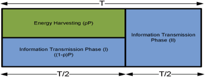
SWIPT: Power splitting protocol


6.2 Energy Harvesting Models
EH models are basically classified as linear and nonlinear based on the relation between the RF signal power and the power of the energy harvester.
6.2.1 Linear Energy Harvesting
Linear EH is a de facto standard in various seminal works [8, 11]. In linear EH, the power of the energy harvester is directly proportional to the RF signal power which increases linearly with the input RF signal power. In practice, the devices are nonlinear devices which include active elements such as diodes and transistors, and hence, EH circuits exhibit saturation for a long duration of input power exposure. Since the RF signal is random, thus power harvested is dynamic. If the input signal power falls below the threshold, EH drops to zero and affects the sensitivity of the circuit [22].
6.2.2 Nonlinear Energy Harvesting
There are various seminal works on nonlinear harvesting models to characterize the practical EH circuits based on piece-wise linear function, rational function, a polynomial function, and a sigmoid functions. In piece-wise linear model, linear response is assumed up to the saturation level to capture the practical EH circuit saturation effect [23]. In rational model, seven parameters are used to characterize the nonlinear effect which are determined by curve fitting with measured data [24]. This model is analytically non-tractable. In polynomial model, the diode output is approximated with truncated Taylor expansion [25]. In sigmoid mode, the relation between input RF signal power and output energy harvested power is modeled with a sigmoid function to capture the saturation effect. However, this model fails to retain the sensitivity [26].
6.3 Impact of Imperfect CSI
6.3.1 Mathematical Modeling
Consider a three-terminal device which includes a source (S), relay (R), and the destination (D), where each of these terminal nodes is equipped with multiple antennas. At R node, amplify-and-forward relaying protocol is employed to broadcast the signal to D with the harvested energy [15]. S is considered as a base station, whereas the user equipment (UE) is taken as R and D, respectively. A channel matrix is considered from node P to node Q as H PQ with dimensions N Q × N P, where N P and N Q represent the antenna count at the P and Q nodes, respectively. It is highly deterrent to use multiple active antennas due to the requirement for active RF chains, which are cost, power, and size in efficient. Hence, to retain the MIMO gains, transmit antenna selection (TAS) is used at S and R nodes. Hence, the hardware complexity and cost are reduced; however, performance is retained. In TAS, at the node P, an ith transmit antenna is selected which maximizes the received signal-to-noise ratio (SNR) for broadcasting the information through the channel vector \({\mathbf {h}}_{PQ}^{(i)}\) to the receiver and is given as
where P ∈{S, R}, Q ∈{R, D}, and P ≠ Q. Channel matrix H PQ has the N P channel vectors (\({\mathbf {h}}_{PQ}^{(i)}\)) with dimensions N Q × 1 of each. Minimum mean square error (MMSE)-based estimator is used at the receiver for channel estimation. To visualize the versatility of the channel in the system performance, all are assumed to be modeled by the generalize complex Nakagami-m frequency flat fading channels, \(Nak(M_{L},\hat {\sigma }^2_{\mathbf {H}})\). All the noise vectors are assumed to be modeled by additive white Gaussian noise (AWGN) vectors with mean 0 and variance \({\sigma ^2_{PQ}} {\mathbf {I}}_{N_{Q}}\). CEEs in channel estimation arises due to the improper pilot pattern. Improper pilot pattern results in irreducible error floor in channel estimation. To avoid CEEs, pilot pattern should be performed as a function of coherence time and frequency [27]. The relation between the actual channel (H) and the estimated channel (\(\hat {\mathbf {H}}\)) in the presence of CEE (δ H) is given as
where δ
H is modeled as  and the variance \(\sigma ^2_{\boldsymbol {\delta }}\) is given as
where ρ is the channel correlation coefficient [28]. Variance of the estimated channel is given as \(\sigma ^2_{\hat {\mathbf {H}}}=\sigma ^2_{\mathbf {H}}-\sigma ^2_{\boldsymbol {\delta }}={\rho \sigma ^2_{\mathbf {H}}}\). For harvesting the energy, we consider TS protocol at the R. The system operation completes in two phases. Energy is harvested at R in the first phase, from the received S signals, whereas IP takes place in the second phase.
6.3.1.1 Time Switching Protocol
As discussed, we employ TS protocol to harvest the energy at the R due to its reduced complexity. Entire communication between S and D takes place over a period of (T) time in two phases as shown in Fig. 6.1. The complete time T is divided into αT time and (1 − α)T for energy harvesting and IP. α denotes the fraction of time, 0 < α < 1.
6.3.1.2 Phase 1
In this phase, energy is harvested at R for αT time.
6.3.1.3 Phase 2
In the second phase, communication link is established for the rest over (1 − α)T time. (1 − α)T time is further divided into two \(\frac {(1-\alpha )T}{2}\) equal halves for a dual-hop communication. S broadcasts the information signal to both R and D, simultaneously, in the first \(\frac {(1-\alpha )T}{2}\) time, whereas in the other \(\frac {(1-\alpha )T}{2}\) time, R broadcast S information signal to the D by utilizing the energy harvested in EH phase. The amount of energy harvested relies on the α value which is allocated to harvest the energy. There is a trade-off between the amount of the throughput achieved and energy harvested. Signal received at R and D is given as
respectively, where P s is the transmit power at the S and n SR and n SD are the AWGN vectors corresponding to the respective SR and SD links. It is assumed that \(\mathbb {E}\{x^2\}=1\) [29, 30]. Energy harvested at the R during EH phase is given as [11],
where η is the energy conversion efficiency which is defined by the energy harvesting circuitry and the rectification process [11]. R amplifies the signal received from S to transmit to D through the kth transmit antenna at R with a gain G and is given as [13, 31, 32]
where P R is the transmit power obtained from the energy harvested phase at the R. At D, signal received is given as
where n RD is the AWGN vector corresponding to the RD link. At D, maximum ratio combiner (MRC)-based optimal receiver filter in the MMSE sense is used to combine the signals received in both the hops[32]. At D, the e2e SNR is given as
where \(\hat {\Lambda }^{(i)}_{SD}=\), \({\Omega _{SD}}=(1+{\hat {\sigma }^2_{\boldsymbol {\delta } SD}})\), \( {\hat \sigma }^2_{\boldsymbol {\delta } SD}=\Lambda _{0}\sigma ^2_{\boldsymbol {\delta } SD} \), \(\Lambda _{0}=P/\sigma ^2_N\) with P transmit power and noise variance (\(\sigma ^2_N\)). \(\hat {\Lambda }^{(i,k)}_{SRD}\) is approximated as [28]
where \({\Omega _{SR}}=(1+{\hat {\sigma }^2_{\boldsymbol {\delta } SR}})\), \({\Omega _{RD}}=(\frac {1}{P_s}+{\hat {\sigma }^2_{\boldsymbol {\delta } RD}}) \), \( {\hat \sigma }^2_{\boldsymbol {\delta } SR}=\Lambda _{0}\sigma ^2_{\boldsymbol {\delta } SR} \), \( {\hat \sigma }^2_{\boldsymbol {\delta } RD}=\frac {K_1}{\sigma ^2_{N}}\sigma ^2_{\boldsymbol {\delta } RD} \), \(\Lambda _{SD}^{(i)}=\overline \Lambda _{SD}||{\mathbf {h}}_{SD}^i||{ }^2\), \(\Lambda _{SR}^{(i)}=\overline \Lambda _{SR}||{\mathbf {h}}_{SR}^i||{ }^2\), \(\Lambda _{RD}^{(j)}=\frac {K_1}{\sigma ^2_{N}}||{\mathbf {h}}_{RD}^j||{ }^2\), and \(K_1=\frac {2\eta \alpha }{(1-\alpha )}\). \(\Lambda _{PQ}^{(i)}\) and \(\overline {\Lambda }_{PQ}\) are the instantaneous and average SNRs of PQ link, respectively.
6.3.2 System Performance Metrics
6.3.2.1 Outage Probability
A system is said to be in outage when the desired rate of transmission is greater than the maximum possible error-free rate of transmission [33, 34]. Rate of transmission quantifies the threshold. For a rate, \(R_{th}=\frac {1-\alpha }{2}\log _2(1+\Lambda _{e2e})\) bits/sec/Hz, the closed-form upper-bound expression for the outage probability is given as [13]
The closed-form expressions of \(F_{\hat {\Lambda }_{SD}^{(i)}}(\Lambda _{th})\) and \(F_{\hat {\Lambda }_{SRD}^{(i,j)}}(\Lambda _{th})\) are given in (6.29) which are derived by following the procedure as in [32]. In (6.29), \(\Delta _{1}= \frac {p}{{{\lambda }_{SR}}}(\frac {\Omega _{SR}}{\Omega _{RD}})+\frac {t+1}{{{\lambda }_{RD}}}\), \(\Delta _{2}=\frac {\Omega _{SR} p(t+1)}{\Omega _{RD}{{\lambda _{SR}}}{{\lambda }_{RD}}} \), Δ = q + n + M RD, 𝜗 = z − q + 1, M SD = m SD N D, M SR = m SR N R, and M RD = m RD N D. Further, \( \lambda _{SD}=\frac {\overline \Lambda _{SD}}{m_{SD}}\), \( \lambda _{SR}=\frac {\overline \Lambda _{SR}}{m_{SR}}\), and \( \lambda _{RD}={\frac {K_1}{\sigma ^2_{N}}\text{E}{||{\mathbf {h}}_{RD}^j||{ }^2}}/{m_{RD}}\). ϕ a,b,c is the multinomial theorem coefficient [15].
6.3.2.2 Asymptotic Analysis
Asymptotic analysis provides the system deep insights which are useful in modeling the system. It provides information regarding system parameters such as diversity and coding gain which are vital in evaluating the performance of the system. By taking the high SNR approximation of e x and K 𝜗(z) [35, eq. (1.211.1), Eq. (8.446)], the closed-form asymptotic outage probability expression is derived at \(\overline {\Lambda } \rightarrow \infty \) as [13]
For i = 1, PQ = SD, for i = 2, PQ = SR, and for i = 3, PQ = RD. Further, O 1 = M SD N S + M SR N S, O 2 = M SD N S + M RD N R, O 3 = M SD N S + MN R, M = m SR N S = m RD N D, and \(k_{PQ}=\frac {\overline {\Lambda }_{PQ}}{\overline {\Lambda }}\).
6.3.2.3 Throughput Analysis
For a fixed transmission rate, throughput is evaluated in delay-limited transmission mode from the outage probability as [11]
where \(\Lambda _{th}=2^{\frac {2R_{th}}{1-\alpha }}-1\) is the threshold SNR for a fixed rate R th.
6.3.3 Results and Discussion
In this section, modeled system performance is validated and discussed through the derived analytical expressions of outage probability and asymptotic outage probability and the Monte Carlo simulations. In the system performance analysis, the parameters are considered as follows: channel correlation coefficients are taken as {ρ SD, ρ SR, ρ RD}, and CSI parameters are considered as ρ = 0.99 for perfect case and ρ = {0.95, 0.9} for imperfect cases. Further, EH efficiency factor (η = 1) and different values of α are considered.
In Fig. 6.3, outage probability results are presented for the 2 × 2 × 2 AC with FP {1, 1, 1} with α = 0.2. In this analysis, three different scenarios are considered such as {0.99, 0.99, 0.99}, {0.95, 0.95, 0.95}, and {0.9, 0.9, 0.9}. Results illustrate the well agreement of the derived analytical results of outage probability and asymptotic outage probability and verified through Monte Carlo simulations. Curves illustrate that the performance of the system is better even after harvesting the energy for α = 0.2. Curves at high SNR regime illustrate the loss in diversity order of the system with a constant error floor for a minor change in CEE values. This is due to SNR independent CEE variance.

2 × 2 × 2 MIMO AC: Outage probability vs SNR for different CEE conditions [13]
In Fig. 6.4, for 2 × 1 × 2 AC with {1, 2, 1} FPs, outage probability analysis is presented to visualize the impact of α under different symmetric CEE conditions. In Fig. 6.4, analytical results of outage probability are presented. The curves demonstrate the degradation of system performance with the increase in α value. With the increase in EH time, error floors increase, and it still increases with the reduction in ρ PQ values. As α increases, EH time increases resulting in a lower IP time, and thus outage probability increases. For an outage probability of 10−3 with α = 0.2, SNR gain of 6 dB is observed for the system with {0.99, 0.99, 0.99} over {0.95, 0.95, 0.95} case. As α value increase to 0.5, SNR gain increases to 10 dB for an outage probability of 10−2. It escalates to ∞ gain for α = 0.7 over {0.95, 0.95, 0.95} case with a constant error floor.

2 × 1 × 2 MIMO ACs: Outage probability vs SNR for different α values [13]
In Fig. 6.5, 2 × 2 × 1-{1, 1, 2} AC throughput is attained by the system which is presented for different CEE values at different rates. Curves illustrate that for R th = 1 bps/Hz, the system throughput attains saturation with τ ∼ 0.4 at 12 dB and 15 dB, respectively, for {0.99, 0.99, 0.99} and {0.9, 0.9, 0.9} cases. For R th = 2 bps/Hz, the throughput of the system saturates to ∼0.7 at 22.5 dB approximately for {0.99, 0.99, 0.99} case, whereas for imperfect CSI case of {0.9, 0.9, 0.9}, system throughput saturates to <0.3 at ≈30 dB. It illustrates the adverse effect of both imperfect CSI and the high data rates over the system performance.

2 × 2 × 1 MIMO AC: Throughput vs SNR in the presence of imperfect CSI conditions [13]
6.4 Impact of Outdated CSI
In the earlier section, the impact of imperfect CSI over the SWIPT-enabled D2D communications is analyzed. In this section, the outdated CSI and its affects are considered in the analysis. As all the nodes are multi-antenna nodes, the effects of outdated CSI over antenna selection and the EH are important metrics of concern. SWIPT-enabled D2D communications in the presence of feedback error are also highly motivated. Hence, in this section, we present the effects of feedback delays and EH in the analysis of an overlay non-regenerative D2D MIMO relay system over generalized Nakagami-m fading channels. System performance is investigated through outage probability and asymptotic outage probability expressions. For a delay-limited transmission mode, throughput of the system is presented.
6.4.1 Mathematical Modeling
To model the feedback errors, consider a scenario where the CSI received at the transmitter is outdated due to the time-varying nature of the channel when fed back from the receiver. Thus, the resultant CSI at the transmitter is outdated and results non-zero feedback link delay. Let’s consider \(\hat {\mathbf {h}}^{u}_{PQ}\) an estimated channel vector to be the delayed channel of \({\mathbf {h}}^{u}_{PQ}\) and which is used in antenna selection. For decoding, consider \({\mathbf {h}}^{u}_{PQ}\) be the estimated channel vector used. Hence, \(\hat {\mathbf {h}}^{u}_{PQ}\) is conditioned over \({\mathbf {h}}^{u}_{PQ}\) following a Gaussian distribution. Thus, the relation between \(\hat {\mathbf {h}}^{u}_{PQ}\) and \({\mathbf {h}}^{u}_{PQ}\) is given as [36]
where ρ PQ is the correlation coefficient between \(\hat {\mathbf {h}}^{u}_{PQ}\) and \({\mathbf {h}}^{u}_{PQ}\). The error is considered to be modeled as \(\mathbf {e}\sim \mathcal {N}(0,I)\) [36].
With Doppler frequency (f d) and delay spread (T d) of the feedback channels, the channel correlation coefficient for Clarke’s fading spectrum is modeled as \(\rho _{PQ}=\mathcal {J}_o(2\pi f_d T_d)\). Further, at R energy is harvested through TS protocol from the S received signals. Energy harvesting and the IP take place as discussed in the earlier section. In the first hop, S transmits the signal with transmit power P S to R and D, respectively. The signals received at multiple antennas at R and D MRC receiver are used, and thus the received signals at R and D are given as
where w SR and w SD are the AWGN vectors corresponding to the SR and SD links, respectively. In the second hop, R broadcasts the received S signal to D after amplifying with a gain by TAS through vth antenna [37]
and is given as
where P R is transmit power at R and w RD is the RD link AWGN vector. P R is drawn from the EH phase as [11]
Signals received from both the hops at D are combined using MRC with a MMSE filter [32, 38]. Thus, the e2e SNR at D is given as
where \(\Lambda _{SD}^{(u)}=\overline \Lambda _{SD}||{\mathbf {h}}_{SD}^u||{ }^2\), \(\Lambda _{SR}^{(u)}= ||{\mathbf {h}}^{u}_{SR}||{ }^2\), \(\Lambda _{RD}^{(v)}= \Lambda _{K_1}||{\mathbf {h}}^{v}_{RD}||{ }^2\), and \(\Lambda _{K_1}=\frac {P_{S}}{\sigma _{N}^2} K_1 \).
6.4.2 System Performance Metrics
6.4.2.1 Outage Probability
As the outage probability determines the reliability of the communication link, it can be analyzed through the closed-form UB expression and is given as [14]
where
Further, \(\Delta _{1}=\frac {e+1}{\lambda _{SD}[1+e(1-\rho _{SD})]}\), \(\Delta _{2}=\frac {a+1}{\lambda _{SR}[1+a(1-\rho _{SR})]}\), \(\Delta _{3}=\frac {p+1}{\lambda _{RD}[1+p(1-\rho _{RD})]}\), Δ5 = Δ2 + Δ3, and Δ6 = Δ2 Δ3. Furthermore, Δ4 = M RD + r + i − 1, 𝜗 = s − i + 1, M PQ = m PQ N Q, and \(\lambda _{PQ}=\frac {\overline {\Lambda }_{PQ}}{m_{PQ}}\).
6.4.2.2 Asymptotic Analysis
As discussed earlier, asymptotic analysis provides the system design insights such as diversity gain and coding gain. Diversity gain provides the number of independent paths between the transmitter and the receiver. Asymptotic outage probability expression is derived at \(\overline {\Lambda } \rightarrow \infty \) as [14]

where diversity order is given by d 1, d 2, and d 3. Further, M = M SR = M RD, d 1 = M SD + M SR, d 2 = M SD + M RD, and d 3 = M SD + M. Furthermore, \(k_{SD}=\frac {\overline {\Lambda }_{SD}}{\overline {\Lambda }}\), \(k_{SR}=\frac {\overline {\Lambda }_{SR}}{\overline {\Lambda }}\), and \(k_{RD}=\frac {\overline {\Lambda }_{RD}}{\overline {\Lambda }}\).
6.4.2.3 Throughput Analysis
We consider a delay-limited transmission mode for the analysis of throughput. Thus, in this mode throughput is evaluated for a fixed transmission rate R r =log2(1 + Λe2e) bits/s/Hz from the outage probability as
6.4.3 Results and Discussions
In this section, we discuss the derived analytical expressions from the various system design aspects and validate them through the Monte Carlo simulations. The system modeling parameters are considered as follows: correlation parameters (CPs) as {ρ SR, ρ RD, ρ SD}, transmission rate R r = 3 bits/s/Hz, and EH efficiency factor (η = 1). In the analysis, urban macro-cell network environment is considered with path loss exponent 4 [39].
6.4.3.1 Impact of MIMO Antenna System
In Fig. 6.6, outage probability and SNR curves are presented for 2 × 2 × 2 AC with FPs, {1, 1, 1}, 1 × 2 × 2 AC with FPs {2, 1, 1} and 1 × 1 × 1 AC with FPs {1, 1, 1}. In the analysis, EH is performed for α = 0.2T, and CPs are taken as {0.9, 0.9, 0.9}. The derived analytical UB results match well with the asymptotic results, and Monte Carlo results validate them. Curves illustrate that for an outage probability of 10−5, 2 × 2 × 2 AC performs better than 1 × 2 × 2 AC with a SNR gain of ≈ 3 dB. For an outage of 10−2, 1 × 2 × 2 and 2 × 2 × 2 ACs have a SNR gain of ≈ 20 dB over {1, 1, 1} AC. This illustrates the improvement of system performance with MIMO antennas.

Outage probability vs SNR for different MIMO ACs [14]
6.4.3.2 Impact of Feedback Delays
In Fig. 6.7, the impact of feedback delays is visualized with respect to (α) over the outage probability at 15 dB SNR for a 2 × 2 × 2 AC with FPs {1, 1, 1}. Curves demonstrate the severity of feedback delays over the outage probability with respect to α. For α < 0.4T, system records lower outage probability with better performance. However, with a decrease in ρ PQ, outage probability increases and results in system performance degradation. Curves illustrate for α < 0.1, system with {0.1, 0.1, 0.1} CP records high outage probability over the other CPs values. Further, system with {0.9, 0.9, 0.9} CP has low outage probability for α < 0.5T. It is noticed that system performance improves with the decrease in αTdue to more IP time.

2 × 2 × 2 MIMO AC: Outage probability vs (α) for different ρ values [14]
6.4.3.3 Throughput Analysis
In Fig. 6.8, throughput vs SNR curves are plotted for a 1 × 2 × 2 AC with FPs {2, 1, 1}. Throughput is analyzed at two fixed transmission rates R r = 1 and R r = 2 bits/s/Hz and with α = 0.2T. Curves illustrate the increase in system throughput with the increase in R r at high SNR. System with {0.9, 0.9, 0.9} CP with an SNR gain of ≈ 5 dB attains higher throughput prior to {0.1, 0.1, 0.1} CP. For R r = 2 bits/s/Hz, system with {0.9, 0.9, 0.9} and {0.1, 0.1, 0.1} CPs, throughput saturates to 0.8 at 38 dB and 43 dB, respectively, whereas for R r = 1 bits/s/Hz, system throughput saturates to 0.4 at 10 dB and 15 dB, respectively.

1 × 2 × 2 MIMO AC: Throughput vs SNR [14]
6.5 Conclusion
In this chapter, concepts of energy harvesting are discussed such as energy harvesting sources, energy transmission techniques, energy harvesting models, and the impact of channel estimation errors over SWIPT devices. Among the available energy harvesting sources, radio frequency signal-based EH finds a viable solution for energy-constraint nodes. The state-of-the-art EH with cooperative D2D MIMO relaying in the presence of channel estimation errors including feedback delays and imperfect CSI is addressed. System performance is quantified through system metrics such as outage probability and asymptotic outage probability. Further, actual data delivery rate is analyzed through the throughput analysis for a delay-limited transmission, and useful insights are drawn. Impact of MIMO antennas, fading parameters severity, severity of the feedback error, imperfect CSI, and energy harvesting time constant over the system performance are also analyzed.
6.5.1 Summary
A brief summary is as follows:
-
Impact of imperfect CSI and feedback delays over MIMO D2D system with SWIPT is analyzed.
-
System performance is quantified through the outage probability and asymptotic outage probability closed-form expressions.
-
Actual delivered data rate is analyzed through throughput analysis.
-
Results illustrate that the system performance degrades with the increase in α values. However, for smaller values of α, system performs better in both perfect and imperfect CSI scenarios.
-
Results illustrate that for α < 0.4T, system attains low outage probability.
-
At high rates, curves demonstrate that the system performance degrades under imperfect CSI conditions.
-
Increase in outdated CSI deteriorates the system performance drastically.
-
Diversity order of the system is lost with a slight increase in CEE, due to SNR independent CEE variance.
-
Impacts of multiple antennas and fading parameters severity along with imperfect CSI are analyzed along with SWIPT.
References
G. Forecast, Cisco visual networking index: global mobile data traffic forecast update, 2017–2022. Update 2017, 2022 (2019)
P. K. Singya, P. Shaik, N. Kumar, V. Bhatia, and M.-S. Alouini, A Survey on Higher-Order QAM Constellations: Technical Challenges, Recent Advances, and Future Trends. IEEE Open J. Commun. Soc. 2, 617–655 (2021)
M. Series, IMT vision–framework and overall objectives of the future development of IMT for 2020 and beyond. Recommendation ITU 2083, (2015)
A. Gupta, R.K. Jha, A survey of 5G network: Architecture and emerging technologies. IEEE Access 3, 1206–1232 (2015)
Y. Chen, Energy Harvesting Communications: Principles and Theories (Wiley, Hoboken, 2019)
V. Leonov, Thermoelectric energy harvesting of human body heat for wearable sensors. IEEE Sensors J. 13(6), 2284–2291 (2013)
P. Grover, A. Sahai, Shannon meets Tesla: Wireless information and power transfer, in IEEE International Symposium on Information Theory (IEEE, Piscataway, 2010), pp. 2363–2367
H. Ju, R. Zhang, Throughput maximization in wireless powered communication networks. IEEE Trans. Wireless Commun. 13(1), 418–428 (2013)
S. Bi, C.K. Ho, R. Zhang, Wireless powered communication: opportunities and challenges. IEEE Commun. Mag. 53(4), 117–125 (2015)
L.R. Varshney, Transporting information and energy simultaneously, in 2008 IEEE International Symposium on Information Theory (2008), pp. 1612–1616
A.A. Nasir, X. Zhou, S. Durrani, R.A. Kennedy, Relaying protocols for wireless energy harvesting and information processing. IEEE Trans. Wirel. Commun. 12(7), 3622–3636 (2013)
T. Li, P. Fan, K.B. Letaief, Outage probability of energy harvesting relay-aided cooperative networks over Rayleigh fading channel. IEEE Trans. Veh. Technol. 65(2), 972–978 (2015)
P. Shaik, P.K. Singya, N. Kumar, K.K. Garg, V. Bhatia, On impact of imperfect CSI over SWIPT device-to-device (D2D) MIMO relay systems, in SPCOM (IEEE, Piscataway, 2020), pp. 1–5
P. Shaik, P.K. Singya, K.K. Garg, V. Bhatia, Outage Probability analysis of SWIPT device-to-device MIMO relay systems with outdated CSI, in IEEE Wireless Communications and Networking Conference (WCNC) (IEEE, Piscataway, 2021), pp. 1–6
S. Parvez, P.K. Singya, V. Bhatia, On ASER analysis of energy efficient modulation schemes for a device-to-device MIMO relay network. IEEE Access 8, 2499–2512 (2019)
P. Shaik, P.K. Singya, V. Bhatia, On impact of imperfect CSI over hexagonal QAM for TAS/MRC-MIMO cooperative relay network. IEEE Commun. Lett. 23(10), 1721–1724 (2019)
T.M. Hoang, X.N. Tran, N. Thanh, et al., Performance analysis of MIMO SWIPT relay network with imperfect CSI. Mobile Netw. Appl. 24(2), 630–642 (2019)
P. Shaik, K.K. Garg, V. Bhatia, On impact of imperfect channel state information on dual-hop nonline-of-sight ultraviolet communication over turbulent channel. Opt. Eng. 59(1), 1–14 (2020)
Y. Alsaba, S.K.A. Rahim, C.Y. Leow, Beamforming in wireless energy harvesting communications systems: a survey. IEEE Commun. Surv. Tut. 20(2), 1329–1360 (2018)
S. Bisen, P. Shaik, V. Bhatia, On performance of energy harvested cooperative NOMA under imperfect CSI and imperfect SIC. IEEE Trans. Veh. Technol. 70(9), 8993–9005 (2021)
A.S. Parihar, P. Swami, V. Bhatia, Z. Ding, Performance analysis of SWIPT enabled cooperative-NOMA in heterogeneous networks using carrier sensing. IEEE Trans. Veh. Technol. 70, 1–1 (2021)
D. Wang, F. Rezaei, C. Tellambura, Performance analysis and resource allocations for a WPCN with a new nonlinear energy Harvester model. IEEE Open J. Commun. Soc. 1, 1403–1424 (2020)
Y. Dong, M.J. Hossain, J. Cheng, Performance of wireless powered amplify and forward relaying over Nakagami-m fading channels with nonlinear energy Harvester. IEEE Commun. Lett. 20(4), 672–675 (2016)
Y. Chen, K.T. Sabnis, R.A. Abd-Alhameed, New formula for conversion efficiency of rf eh and its wireless applications. IEEE Trans. Veh. Technol. 65(11), 9410–9414 (2016)
B. Clerckx, E. Bayguzina, Waveform design for wireless power transfer. IEEE Trans. Signal Proces. 64(23), 6313–6328 (2016)
E. Boshkovska, D.W.K. Ng, N. Zlatanov, R. Schober, Practical non-linear energy harvesting model and resource allocation for SWIPT systems. IEEE Commun. Lett. 19(12), 2082–2085 (2015)
M.K. Ozdemir, H. Arslan, Channel estimation for wireless ofdm systems. IEEE Commun. Surv. Tut. 9(2), 18–48 (2007)
M. Seyfi, S. Muhaidat, J. Liang, Amplify-and-forward selection cooperation over Rayleigh fading channels with imperfect CSI. IEEE Trans. Wirel. Commun. 11(1), 199–209 (2011)
K.K. Garg, P.K. Singya, V. Bhatia, Performance analysis of NLOS ultraviolet communications with correlated branches over turbulent channels. IEEE/OSA J. Opt. Commun. Net. 11(11), 525–535 (2019)
K. Garg, P. Shaik, V. Bhatia, O. Krejcar, On the performance of relay assisted hybrid RF-NLOS UVC system with imperfect channel estimation. J. Optical Commun. Netw. (2021). [Online]. Available: https://doi.org/10.1364%2Fjocn.440819
Y. Liu, L. Wang, M. Elkashlan, T.Q. Duong, A. Nallanathan, Two-way relay networks with wireless power transfer: design and performance analysis. IET Commun. 10(14), 1810–1819 (2016)
P. Shaik, P.K. Singya, V. Bhatia, Performance analysis of QAM schemes for non-regenerative cooperative MIMO network with transmit antenna selection. AEU-Int. J. Electron. Commun. 107, 298–306 (2019)
J. Jose, P. Shaik, V. Bhatia, VFD-NOMA under imperfect SIC and residual inter-relay interference over generalized Nakagami-m fading channels. IEEE Commun. Lett. 25, 646–650 (2020)
K.K. Garg, P. Shaik, V. Bhatia, Performance analysis of cooperative relaying technique for non-line-of-sight UV communication system in the presence of turbulence. Opt. Eng. 59(5), 055101 (2020)
I.S. Gradshteyn, I.M. Ryzhik, Table of Integrals, Series, and Products (Academic, New York, 2014)
N. Yang, M. Elkashlan, P.L. Yeoh, J. Yuan, Multiuser MIMO relay networks in Nakagami-m fading channels. IEEE Trans. Commun. 60(11), 3298–3310 (2012)
S. Parvez, D. Kumar, V. Bhatia, On performance of SWIPT enabled two-way relay system with non-linear power amplifier, in NCC (IEEE, Piscataway, 2020), pp. 1–6
V. Bhatia, B. Mulgrew, Non-parametric likelihood based channel estimator for Gaussian mixture noise. Signal Process. 87(11), 2569–2586 (2007)
A. Goldsmith, Wireless Communications (Cambridge University Press, Cambridge, 2005)
Author information
Authors and Affiliations
Editor information
Editors and Affiliations
Rights and permissions
Copyright information
© 2023 The Author(s), under exclusive license to Springer Nature Switzerland AG
About this chapter

Cite this chapter
Shaik, P., Bhatia, V. (2023). Energy Harvested Device-to-Device MIMO Systems for Beyond 5G Communication. In: Matin, M.A. (eds) A Glimpse Beyond 5G in Wireless Networks. Signals and Communication Technology. Springer, Cham. https://doi.org/10.1007/978-3-031-13786-0_6
Download citation
DOI: https://doi.org/10.1007/978-3-031-13786-0_6
Published:
Publisher Name: Springer, Cham
Print ISBN: 978-3-031-13785-3
Online ISBN: 978-3-031-13786-0
eBook Packages: Computer ScienceComputer Science (R0)