Modeling of Biological Systems: From Algebra to Calculus and Computer Simulations

Abstract

In this chapter we present a survey of mathematical modeling approaches to biological problems. We approach the modeling efforts through several mathematical techniques: from basic algebra, already studied in middle- and high school, to calculus, at the transition of high school and college. Throughout the chapter, we rely heavily on computer simulation techniques with which we investigate different aspects of these models and their relationships with the studies systems, illustrating the modern approach of computational thinking. We have presented versions of these problems and models in our own courses in mathematics for non-majors, targeted to first- and second-year colleges students who are interested in biology and life sciences. Many students have told us that they found the approach engaging and that it increased their appreciation of mathematics as an applied science. The problems and project that you will see here are selected from areas of population biology (populations of squirrels, insects, flies, and wasps); use of medical sensing and modeling to detect the blood pressure and heartbeat in patients; and epidemiology, modeling the spread of infectious diseases, from Ebola in West Africa, with an option to study the COVID pandemic in 2020–2021.

FormalPara Suggested Prerequisites

The sections are ordered in increasing difficulty of conceptual ideas and technical tools. You do not need to read or try them in the indicated order, but if we use concepts from prior section, look them up as needed. In the first two sections we expect acquaintance with the ideas of basic algebra, in particular, with the more advanced concepts of sequences and relationships between their terms. The subsequent two sections start using concepts from differential calculus. Some familiarity with that field would be helpful, although we do provide some guidance. All problems use some form of computational thinking, which involves computer programming. Initially that is in Excel, assuming familiarity with functions and formulas. Then we transition to modeling tools that are used more broadly by practitioners, like Octave and Matlab. We provide links to tutorials for the use of these systems.

1 Introduction

Mathematical models allow us to pause and reflect on all the “what ifs” and “I wonders” we might have about our universe. In this chapter, you will read about several different ways mathematical models are used to answer questions. Questions like, how to measure someone’s heart rate without touching them, how two insect populations relate to crop yield, and more!

1.1 A Description of Mathematical Modeling

Mathematical modeling is a cyclic and iterative process—a delicate dance between making and challenging assumptions. When building models, there is rarely a “right” answer—only answers that stand on specific assumptions are supported by mathematical logic and principles and help us generate productive knowledge in the given context and setting. To help make sense of what can be a difficult process to explain and understand, we frame the modeling process in four steps.

Step 1: Goals, Questions, and Assumptions

What do you want to know? What do you already know? Predictions and analyses stemming from models are only as valuable as the accuracy of the assumptions. We must think carefully about any assumptions we make and the criteria outlined in problems we are given to solve.

Step 2: Build a Model

How can you utilize mathematics (and other fields) to move from your assumptions to the answers to your questions? What areas of mathematics will be most useful? From what subjects can you draw inspiration?

Step 3: Apply your Model

Use the model to answer questions and meet initial goals.

Step 4: Assess and Revise your Model

Are the results/implications reasonable? What happens when you alter various assumptions? Reflect on whether the assumptions posed are accurately incorporated and whether there might be additional constraints to be considered. Can the model be more accurate or efficient? Does it need to be?

We do not mean to imply that you should always proceed linearly from Step 1 through to Step 4. Sudden realizations about the mathematics involved or the phenomenon to be modeled may send you back to a specific part of your model immediately. New data from the field may stop you in your tracks to revise essential assumptions. However, the general structure and spirit of these steps supports an iterative approach to mathematical modeling in which answers are not “right,” but well-supported. These steps and our general approaches are not unique to these projects. They parallel directly George Polya’s four principles of problem-solving [1] and are found embedded in the description of mathematical modeling from the Society for Industrial and Applied Mathematics [2]. Look for this cycle within your own pursuits!

1.2 Building a Model with Bias

There is inherent bias in mathematical modeling. Our decisions regarding what to study and how to go about studying it are subject to our bias as people. Bias is not something that can be temporarily suspended or minimized—it is inherent to us. Acknowledging our bias and exploring the implicit bias in data does not diminish our results, it strengthens them by allowing us to situate our results appropriately with full awareness of the shortcomings and advantages of the model. As an example, medical research has historically been done exclusively on adult male subjects. In 2015 the United States Food and Drug Administration mandated that clinical trials include female participants. The impact of that methodological decision includes we are still today learning how differently women experience medical emergencies such as heart attacks [3]. This bias was inherent within society as well as within the research community and thus not accounted for in making recommendations.

1.3 A Note About Computer-Based Simulations

All files with instructions for computer simulations are available for download at the GitHub repository typically used for such tasks [4]. We typically develop and share our code in this manner, although the use of repositories like GitHub becomes more obvious after much more experience with coding. For now, just take our word that it is a good idea to learn how to use them.

The first two sections illustrate the use of computer-based simulations for mathematical modeling using simpler and more widely accessible platforms like Microsoft Excel and Google Sheets. Those platforms have the benefit of familiarity and ease of entry, but they are severely limited when problems scale up in size and complexity, becoming progressively more difficult to use, if at all.

Not surprisingly, the professional math modeling community is typically using different platforms in our day-to-day work. They tend to be more difficult to learn and master but allow us to tackle much more complex problems. Sections 4 and 5 present examples in two of these platforms: the commercial MATLAB [5] and the open-source GNU Octave [6]. They have similar capabilities mainly because Octave was specifically created to be compatible with MATLAB and use MATLAB commands and structures without many changes. The main difference currently is that MATLAB provides a nice integrated environment in which one can mix text, computations, and visualizations, while Octave still uses text-based work environment in which results have to be collated to separate documents with some additional effort. One emerging platform which bridges some of the gap between integrated ease of use and open source/free accessibility is Python in Jupyter Notebook [7, 8]. We note that in passing but will not provide additional details in this chapter.

Since both MATLAB and Octave are based on a text-based programming model, we usually direct our students to online tutorials which provide them the foundations of working with these systems and provide them with additional online materials to expand their expertise should they want to. We believe that the basic tutorials provide sufficient material so students can start exercises and later extend their knowledge in the context of problems on which they are working and engaged. MathWorks, the company behind MATLAB, provides a nice free introductory tutorial [9], which awards certificates to students after they finish it. We usually assign that tutorial as homework on our first day of class and collect the certificates. The same tutorial will provide basic familiarity with Octave as well, but there will be differences in the user interface. As an open-source product, Octave does not have the polished tutorials of MATLAB, but there is still a lot of documentation in the form of a Wiki, and several good quality video tutorials, comparable to MATLAB’s Onramp [10], that can serve the same purpose.

We recommend that, before you attempt Sects. 4 and 5, you install MATLAB or Octave on your computer, engage with the tutorials, while trying to replicate what they suggest on your system, and continue with the those sections after you finish those tutorials.

1.4 Active Learning

Learning is not a passive activity. To sit and read the words that follow will impart knowledge, no doubt. But to learn about mathematical modeling, one must actively model. Research in the teaching and learning of mathematics, science, and engineering shows consistently that active learning in the classroom leads to improved student learning [11]. When reading a text like this, you are your own teacher in many ways. Teach yourself well! We encourage you to try out the examples provided and explore in new directions. Alter parameters and think about the implications. Adjust assumptions to fit a new space and play with the ideas as you read. This is active learning (and reading!). This philosophy also defines in part the structure of this chapter and its section. Unlike the majority of chapters in this book, we chose to not initially develop “all necessary math” and then present you with challenges and research problems in which to use “it.” We chose to state a potential problem relatively early in the corresponding section, then discuss some possible mathematical approaches to it and provide references for specific tools that the reader can follow as needed. This approach allows us to follow our favorite learning strategy, which we use in our work as modelers as well: a combination of foundation learning of general mathematical structures and “just in time” learning of specific mathematical tools that could be of use to a particular problem.

2 Grey Squirrels in Six Fronts Park: Modeling a Changing Population

Section Author

William Hall

Suggested Prerequisites

Algebra, sequences, difference equations

In this section, we build and use a mathematical model using spreadsheet software to explore how a population of grey squirrels changes over time given various parameters and observations. This problem is fictional—it was built for the purposes of instruction so that the mechanics of translating the problem into the mathematical model can be centered in the discussion. In the projects that follow, the contexts and mathematical models are authentic and the principles are illustrated outside a fictional park.

2.1 The Problem

Problem 1

A population of grey squirrels is being tracked within Six Fronts Park. In a recent survey of park wildlife, it was estimated there were 1000 squirrels in the park. The squirrel population has been increasing as of late and city officials have asked for a report. Specifically, they want to know when they can expect the squirrel population to reach 2000.

2.1.1 Step 1: Goals, Questions, and Assumptions

We are asked to estimate when the population of grey squirrels will reach 2000. We are told to assume the squirrel population is increasing by 20% each year.

2.1.2 Step 2: Build a Model

Many different models can be built to approximate the given situation and the reader is encouraged to explore those that come to mind. Here, we will use Microsoft Excel to provide a numerical approximation, using difference equations to solve what would be called an initial-value problem in differential equations; however, you will not need experience in differential equations for this activity. See Sects. 4 and 5 for more details on difference equations and differential equations. First, we need to translate our assumptions into mathematical equations and expressions that can be used in our model. We will use S(t) to represent the population of grey squirrels t years from today. We know that we can assume there to be 1000 squirrels in Six Fronts Park today. This is represented in our model as S(0) = 1000, where t = 0 represents the present day. Assuming the growth rate of the squirrel population is proportional to the squirrel population itself and not explicitly dependent on time, we use R(S) to represent the growth rate of the population of grey squirrels for some given population. Note that while S is a function of t, R is a function a S. Assuming a growth rate of 20% per year in the context of the squirrel population can be understood as: if there are 1000 squirrels in the park, the population will be growing at a rate of 1000 ⋅ 0.2 =  200 squirrels per year. In our model, we can write this more generally as R(S) = 0.2 ⋅ S. Given this information, we translate the officials’ question (“When will there be 2000 squirrels?”) to our mathematical notation: Find t such that S(t) = 2000.

What makes this problem challenging (and interesting too!) is that as soon as more squirrels are added to the park, the growth rate increases. In our model: as S increases, so too does R(S). For example, if there were 1200 squirrels in the park, the growth rate would be 1200 ⋅ 0.2 = 240 squirrels per year. How do we approximate a population in flux with a growth rate that changes too? One answer: approximation. If we assume that the growth rate remains constant for some finite interval (e.g., one month, three months, six months) we can approximate how many new grey squirrels the model predicts there will be within that time interval. We can do this several times, updating the rate of change as we approximate the accumulative net change in the number of grey squirrels. A combination of the size of those time intervals and how we approximate the rate of change within each interval will determine how accurate our overall approximation will be. In the next section we will use Excel to apply the model and answer the officials’ question.

2.1.3 Step 3. Apply the Model

The method showcased in this section relies on assuming non-linear growth can be approximated using linear functions over finite time intervals. To find an exact solution, we would need to consider infinitely small chunks of time (and possibly infinitely small squirrels). However, we can approximate the solution with as much accuracy as we like using just spreadsheet software and a few formulas. First, we know that at t = 0, the growth rate is 200 squirrels per year, as we calculated earlier. If we assume this growth rate will remain constant over three months, we can approximate that there will be (200 squirrels per year) ⋅ (0.25 years) =  50 additional squirrels in Six Fronts Park over three months. Now there are approximately 1050 squirrels in the park. At this point, we re-calculate the growth rate since there are more squirrels and we know that more squirrels means faster growth. Now, the population is growing at 1050 ⋅ 0.2 =  240 squirrels per year. After three additional months, (240 squirrels per year) ⋅ (0.25 years) =  60 additional squirrels added during that three-month time interval. Thus, six months from now, we can estimate there to be 1000 + 50 + 60 = 1110 grey squirrels in Six Fronts Park.

We can speed up this process with the help of spreadsheet software (many other software options exist for this type of modeling, but we use Microsoft Excel here). We will track time in the first column, the squirrel population in the second column, and the growth rate with the third (using t, S, and R, respectively, as column headings). The first entry will be the given information, that at t = 0, the population S is 1000. We also need to make note of the time span over which we have decided to assume a constant growth rate, which in our case is three months (0.25 years). Once you have listed this value, you can use the “define name…” feature to assign a character string you can use to call up this value in formulas later on. In this example, I used “dt” as the name for the cell containing 0.25, where dt represents a small change in time. The benefit here, instead of typing 0.25 repeatedly, is that we can change the value in the cell and any formulas in which we have used “dt” will update to the new value. This enables us to explore how our assumption (the growth rate was constant for some finite time interval) impacts the overall approximation for the population of grey squirrels.

To calculate the growth rate at this point, we utilize a formula in Excel and let the software run calculations. In the R column, in the cell adjacent to the current population, we want to compute 0.2 multiplied by the current population. To use a formula, type the equal sign followed by “0.2*” then you can either click the cell with the current population or type the cell location directly. This is illustrated in Fig. 1.

Fig. 1

Using excel to calculate the growth rate

Moving to the next row, we first use how much time has elapsed (0.25 years) to give the next value for t. To do so, we use a formula in the next cell in the time column to add the value of “dt” we set earlier (0.25) to our previous time (t = 0). Next, we update the number of squirrels in the park after this period (0.25 years) by approximating the number of new squirrels by multiplying the current growth rate by the value saved as “dt” and adding it to the previous population (see Fig. 2 for formulas).

Fig. 2

Formulas for calculating time and population

Finally, to find the new growth rate after 0.25 years have passed and there are now approximately 1050 squirrels in the park, we use the fill-down feature (click and drag the square in the bottom right corner of the cell with the formula you want to apply). With the first two rows now filled in, if you simultaneously select all three cells in the second row of values, you can use the same fill-down feature to generate approximations as far into the future as you desire. See Fig. 3 for Excel formulas.

Fig. 3

Formulas for model of population of grey squirrels

According to the current model (see Fig. 4), the squirrel population should reach 2000 between 3.5 and 3.75 years from now.

Fig. 4

Model of population of grey squirrels with constant growth rate for 0.25 year periods

2.1.4 Step 4. Assess and Revise Your Model

What would happen if we assumed the growth rate was constant for one month instead of three? Here we replace 0.25 with 0.083 (approximately $\frac {1}{12}$). Make a mental conjecture about how the solution might change before reading further or changing your own values. Since we assigned “dt” to represent whatever value is in the cell marking our time span, we can change that value and the entire model will update as well. However, you may need to highlight the bottom row and use the fill-down feature to include more rows in the model. In this model, our approximation for when the population will hit 2000 falls between 3.486 and 3.569 years from today. This interval is earlier than the previous one we found. Does that match your conjecture?

2.2 Conclusion and Exercises

In this section, we modeled the population of grey squirrels in a fictional park using numerical approximation methods. There are many ways to alter this model to pose and answer new questions. Below, you will find several exercises the reader can undertake within the fictional space of the park. Elevating to the level of project could include utilizing the modeling techniques here in analyzing publicly available data (e.g., COVID-19 infection/vaccination rates, unemployment rates) to pose and reflect on questions about critical social issues in one’s community.

Exercise 1

Imagine you found out there was an error in the initial report and there were only 800 squirrels in the park at t = 0. How does this alter the results of your model under the original assumption? When would the population hit 2000 in that case?

Exercise 2

What if a fire caused a significant drop in the population growth rate during the first six months of the second year? How could you use the spreadsheet we built here to model this case?

Exercise 3

Pose your own “what-if” question and then reflect on the results. What do you learn about both the context and your model?

3 Non-contact Cardiovascular Measurements

Section Authors

Giovanna Guidoboni and Raul Ivernizzi

Suggested Prerequisites

Algebra, spreadsheet

3.1 Context

At every heartbeat, blood is ejected from the heart into the cardiovascular system, generating a thrust that is capable of moving our whole body [12]. This motion can be captured via external sensors, such as accelerometers placed in an armchair or load cells placed under the bed posts. Precisely, these sensors capture the motion of the center of mass (which is the unique point of a distribution of mass in space to which a force may be applied to cause a linear acceleration without an angular acceleration) of the human body resulting from the function of the cardiovascular system, thereby enabling health monitoring without requiring direct body contact. This capability is especially useful for elderly individuals and patients suffering of chronic diseases, such as those suffering of heart failure. What does this have to do with math? Can we reconstruct the position of a known mass placed on the bed by elaborating the signals from the load cells? This is what we will explore in this project. We will see that unexpected results may occur…and yet Euler in his master thesis in 1771 already explained all about it.

3.2 The Challenge

Research Project 1

Imagine that a doctor one day asks you to help him solve a problem. He explains to you that it would be his intention to monitor the health of the cardiovascular system of a patient that is bedridden for good part of the day. The cardiovascular system, he continues, is made of many parts all working together to make sure that every inch of our body gets the blood and the oxygen that it needs to function (see Fig. 5 for a schematic representation of the main parts of the cardiovascular system). The heart is the main pump, beating about 100,000 times and pumping about 7200 liters (1900 gallons) of blood each day through an amazing network of blood vessels of different shape and size.

Fig. 5

The cardiovascular system

As a doctor monitoring patients with cardiovascular problems, it is very important to know whether the patient has a problem in the heart or the blood vessels, because depending on the situation different medicines can be administered or interventions can be pursued.

The doctor says there are already several ways to understand if a person’s heart is working well. For example, you can use the electrocardiogram (often abbreviated to ECG), which consists of measuring the electrical activity of the heart using electrodes placed on the skin (usually on the chest of patients) and provides a graph of voltage versus time. Each peak in the graph corresponds to a heartbeat, and other useful information can be gleaned from the minor peaks (see Fig. 6 for a schematic of the peaks in an ECG graph). In addition to the ECG, the pulse oximeter is another sensor that is often used for patient monitoring (see Fig. 7). This sensor is placed on a finger, as if it were a clothespin, and is able to measure the heart rate and the amount of oxygen in the blood through the emission and subsequent measurement of light beam from a point.

Fig. 6

Standard electrocardiogram (ECG) signal

Fig. 7

Pulse oximeter finger sensor

Our doctor’s idea, however, is to obtain data on the whole cardiovascular system simultaneously, namely including both the heart and the blood vessels, and to do so without touching the body of the patient! In fact, both the ECG and the pulse oximeter require body contact and they have uncomfortable wires that reach a computer capable of processing their signals.

So how can we measure the heartbeat of a subject or other information about his/her cardiovascular system, without applying sensors on him/her? It seems impossible! One could take advantage of the fact that the patient is lying on a bed. So, thinking about it, he/she is touching the bed. Is it possible to use this contact to get some useful information by putting sensors on the bed frame instead of on the patient directly? This is what we will experiment together.

We develop this challenge project in more detail to demonstrate how we work with broadly defined projects like the ones in this book, how we approach them, constrain them and define our own smaller project. Subsequent project in this chapter is meant to be more independent, while still offering some guidance.

3.3 The Initial Experiment

Let us do the following experiment. Take a glass, possibly transparent and with a wide base. Fill it halfway with water and walk to a place where you can safely lie down supine (on the back or with the face upward), such as a sofa or a bed. Lie down carefully, face up, with your head resting on a pillow so that is possible to see your feet without straining abs. Now, place a glass with water on your chest in such a way that is stable enough for it not to tip over. Now if you hold your breath for few seconds and try to remain still you will notice interesting phenomena: the water moves even if you stay still. One can look closely and see that the surface of the water moves periodically, perhaps just a little, but it does. But why does this happen even if we were holding our breath and trying to be immobile?

The answer is: the water move because it is impossible to stay perfectly still, because we have a beating heart inside us!

Every time that the heart ejects blood into our vessels, it generates a thrust that moves our whole body in the opposite direction, thereby displacing the water in the glass. This is Newton’s third law, also known as the action-reaction principle: to every action there is a reaction that is equal in magnitude and opposite in direction. This fact has actually been known for quite some time. Biathlonists or military snipers, for example, train a lot to pull the trigger taking into account this phenomenon. In fact, even if they hold their breath, they cannot stop their heart from making them jump at each beat, so they must learn to synchronize the shot with the beat.

Since the mid-1900s, several scientists were developing instruments to accurately measure these body movements. One of the most popular methods was the “swing bed,” which consisted of a rigid board, suspended by means of cables that were attached to the ceiling or to a stiff metal frame (see Fig. 8). They saw that the power of the cardiac contraction that pushed the blood in one direction was able to move the entire bed with the person on it. These movements were, therefore, simple to be measured. In fact, it was enough to fix a felt-tip pen facing down to the oscillating table, and if you make it so that it touches a sheet of paper placed under it, it will then trace the movement of the bed. The signal generated by the body motion in response to the flow of blood in the cardiovascular system is known as ballistocardiogram, typically abbreviated to BCG. Since then, different and more precise methods have been developed to measure the BCG, for example, using contactless distance meters such as those laser meters that architects use to measure the size of the rooms of a building, or else by using accelerometers. A system made of a bed suspended with cables is quite impractical to be used in a hospital or at home. So, it is natural to wonder if there is a way to measure the forces that create the BCG using a normal bed resting on the ground rather than a suspended one.

Fig. 8

Picture of an old prototype of suspended bed

3.4 Weigh a Bed?

Let us imagine that we have 4 equal scales. In practice, in scientific laboratories, bathroom-like scales have more sophisticated substitutes, which are known as “load cells” (see Fig. 9). They may look different than the standard scales, but essentially they do the same thing: they measure the mass of an object. In addition, these instruments can also be connected to a computer to read the data of the multiple load cells simultaneously and even continuously, obtaining a graph as a function of time. This aspect will come in handy.

Fig. 9

Picture of a load cell placed under the leg of a bed

If we place one load cell under each bed post, for a total of four load cells, we will be able to take into account the weight that each post unloads on the ground. But what do we do with this apparently useless data?

Let us remember that we are interested in having a measure of how the heart makes the body vibrate in order to measure its beats and possibly obtain other useful information. Is it possible, having only the measurement of the “constraint reactions” of the bed to the floor (i.e., the forces that it transmits to the floor and which, in turn, the floor transmits to the bed by reaction), to obtain the forces transmitted by the person’s body to the bed itself? In short, we would like to understand if we can use the load cells to quantify those very same forces that make the water move inside the glass on your chest or make the bed swing when suspended with cables.

The answer is that, thanks to mathematics, it is possible. And it is not very complicated either. Let us see how to get this information:

We draw a diagram of the bed, with the posts at the four corners. We label each corner with a number from one to four. We set a Cartesian reference frame by drawing the x and y along the direction of the bed width and length, as shown in Fig. 10.

Fig. 10

Three-dimensional schematic representation of a bed

We indicate with R ₁, R ₂, R ₃, R ₄, the constraint reactions that the bed exchanges with the floor. Basically these are the forces that we read through the load cells. (Note that the direction towards which we draw the forces is not important at the moment. In fact, we can fix the arrows in any direction and, at the end of the computations, the +  or − sign that we will obtain will automatically change the directions, if necessary). To simplify the computations, let us consider only one direction at a time, either x or y. We are basically choosing to look at the bed either along its width or along its length and we add together the reactions that act on the same end of the segment, as schematized in Fig. 11.

Fig. 11

Cross sectional schematic representation of the forces to which the bed is subjected

Now imagine placing a weight of known mass, say 1 kg, on the bed. We indicate with W _bed the mass of the bed, with W _weight the mass of the small weight and with W _tot the total mass of the bed plus the mass of the small weight. Thus we can write W _tot = W _bed + W _weight. We can represent this situation by drawing a downward arrow representing W _tot, as schematized in Fig. 11 left, or if we consider the two components related to the weight of the bed and that of the weight separately, we obtain Fig. 11 right (which is anyway equivalent to Fig. 11 left).

The question we ask ourselves now is the following: “Using only the data obtained from the load cells under the bed posts, would we be able to reconstruct the position of the small weight on the bed?” This question will be the important for the next reasoning.

If we are able to reconstruct the position of a small weight on the bed, having only the data from the load cells, it would mean that we are able to measure the deviation of the center of mass of the bed if there is a weight on it. This would lead us to say that, if a person were lying on the bed, we would be able to measure the displacements of the person’s center of mass, and these would be caused precisely by the movement of blood inside the arteries. We would have measured the BCG, which provides information about the performance of the whole cardiovascular system!

Returning to our problem, to reconstruct the position of the weight, we use what is called “rotational equilibrium.” In physics and mechanics, the moment of a force is the rotational equivalent of a linear force, and to calculate it we just need to multiply the modulus of the force (i.e., its intensity, in N = “Newton” as unit of measure, for example) by the arm (i.e., the distance perpendicular to the force, expressed in m = “meters,” for example) from a fixed point that we can choose at will and we will call the fulcrum. As a result, we will get the moment of that force relative to the chosen fulcrum, and it will have Nm = “Newton per meter” as unit of measure.

By enforcing the rotational equilibrium with respect to the left end of the bed indicated with a gray point in Fig. 11, we obtain:

(1)

(2)

From the first equation, we can retrieve the location

of the center of mass along the bed width when the weight on it.

For the second equation we need

.

Adding the load cell signal and averaging it over time, we can obtain W _tot. Because W _weight is known, we can obtain

by subtraction:

(3)

To obtain

, we need to write the rotational equilibrium for the bed without the weight on it. Let us denote by R _1,bed, R _2,bed, R _3,bed, and R _4,bed the load cell reactions that we measure in this case. Thus, we can write

(4)

Finally, we can combine the two equations to obtain an expression for the coordinate

identifying the position of the weight along the bed width:

(5)

Repeating the same steps along the y axis, we obtain an expression for the coordinate

identifying the position of the weight along the bed length:

(6)

3.5 Let Us Get Our Hands Dirty!

Exercise 4

Let us now have some fun and use what we have learned so far to reconstruct the position of a small weight placed on a bed, given the readings from four load cells placed under the bed posts. Specifically, let us consider the data reported in the table, compute the coordinates x _c and y _c for each of the weights placed on the bed. Let us assume that the dimensions of the bed are as follows (Fig. 12):

Bed length::

L = 200 cm= 2.0 m (78.74”)

Fig. 12

Table reporting the mass of the weight positioned on the bed, and the magnitude of the constraint reactions of the bed posts measured by the load cells. Note that there are 5 different cases associated with 5 different weights positions. Case #0 is the reference case, where there is no extra weight on the bed

Bed width::

W = 150 cm= 1.5 m (59.055”)

Hint: Notice that in the case #0 no weight was placed on the bed. You can use this case to obtain the information that you need for to calculate W _bed and x _c,bed.

Solution

See Fig. 13, which shows the solution in the form of a table with attached the load diagrams for the five scenarios.

Fig. 13

Table and images showing the solution to the exercise. First the total weight is calculated, then the center of mass of the system (bed + weight) is obtained and, finally, the position of the weight in the four cases is obtained

3.6 Interesting Observations

One would expect that, by adding an extra weight on the bed, all the load cells would record a higher mass. But this is not always the case!

Let us take a second look at the example described in the previous section. In the absence of an extra weight on the bed (see case #0), the load cells in positions 1 and 2 measure 11 kg each, whereas the load cells in positions 3 and 4 measure 9 kg each. Let us now add an extra weight of 1.5 kg on the bed (see cases #1, #3 and #4). In case #1, all the load cells record an increased mass, as we would have expected. However, in case #3 we see that the load cell in position 1 measures R ₁ = 10.375 kg, which is less than 11 kg! We observe a similar phenomenon in the case #4 with the load cell in the position 2, for which R ₂ = 10.775 kg < 11 kg. Interestingly, the extra weight in cases #1, #3 and #4 is the same, but it is placed at different locations with respect to the center of mass of the bed.

This apparently strange behavior can be explained by looking at the following ideal experiment: Let us take a very stiff rectangular board with 4 legs, one at each corner (as a very stiff bed). If two diagonally opposite legs are much longer than the other two (e.g., referring to Fig. 14, assume that legs 2 and 3 are longer), they create a line of equilibrium. As the other two legs are shorter, dropping a weight on one triangular side of the board (for instance, putting the weight close to leg 4) leads to a reduction of the reaction force exerted by the leg opposite to the triangular part chosen (in this case a reduction of the weight at the leg 1). This can also bring, in some cases, to the lifting of the bed corner with respect to its original position.

Fig. 14

Representation of the states of equilibrium of a bed that has two longer transverse legs. Left: unstable equilibrium position with the bed parallel to the ground. Middle: stable equilibrium position with the bed tilted to the right; Right: Position of stable equilibrium, with the bed inclined towards the left leg

We can, therefore, conclude that using a bed with 4 legs, the equilibrium solution is not necessarily unique, because, for example, by placing the weight exactly on the equilibrium line imagined in the ideal experiment explained above, we can obtain that the table naturally rests more on leg 4 or more on leg 1 based on its initial configuration. But both situations are valid.

On the other hand, considering a triangular table with only 3 legs, we immediately understand that there cannot be any stable oscillatory movement between two legs, and, therefore, each equilibrium solution must be unique. In general we can say that for every structure with more than 3 legs on the ground we have a hyperstaticity that generates multiple possible balanced solutions, all equally valid in theory, but only one will appear in practice. This is exactly what Euler studied in his master thesis in 1771!

Challenge Problem 1

Let us now think back at Eqs. (5) and (6). There are many more interesting questions you could explore. Given the same weight, do you think it would be easier or harder to lace it on the bed if the bed’s dimensions are closer to a square, in which case L = W, or to an elongated rectangle in which case L < W or L > W? How do you expect the weight of the object to matter? What are problems that you think you may encounter if the object is very heavy or very light?

3.7 Conclusions

We have seen that it is possible to make measurements of objects placed on a bed using only load cells placed under each post. But what does this have to do with the original question that the doctor asked us? The doctor would have liked to be able to have measurements of cardiovascular health without touching the person. Well, we are now able to say that by analyzing the weight transmitted to the floor by the posts of the bed, we can accurately measure any variation in the center of mass linked to objects placed above the bed. Thus, when a person is on the bed and the blood moves inside the cardiovascular system, we will be able to detect the change of the person’s center of mass based on the load cell readings... and here we have our desired BCG!

All of this was made possible by using mathematics to write down the physics of the system into equations. Scientists have taken this approach even further, by using mathematics to write the equations describing the physics of the blood flow into the cardiovascular system and generate virtual BCGs by simulating on a computer healthy or diseased conditions [13].

Examples of real load cell recordings are reported in Fig. 15 These recordings have been performed within the laboratories of the Center for Eldercare and Rehabilitation Technology directed by Prof. Marge Skubic at the University of Missouri. Data have been collected on a healthy subject (male, 26 y/o). By elaborating the signal from the load cells, it is possible to capture in a very precise manner the heartbeat, see Fig. 15, and the breathing pattern of a subject, see Fig. 16.

Fig. 15

Total weight signal obtained by summing, for each instant, all four load cells measurements. The result is then normalized by the average

Fig. 16

Over-time weight measurement obtained by one load cell placed under a bed leg with a patient on it. The high-frequency peaks are due to the heart rate, while the low-frequency curve (obtained by interpolation) shows the respiration rate

Sensors based on the mathematical principles described in this chapter are not just a mere academic exercise. in their different forms, from load cells to accelerometers and piezoelectric sensors, are helping many people around the world suffering from cardiovascular diseases living their lives as independently as possible while being monitored for potential worrisome conditions. Currently, Prof. Guidoboni is directly involved in helping monitor hundreds of elderly individuals in over 10 long-care facilities. Math does, indeed, help us all live a better life

4 Difference Equations in Population Ecology

Section Authors

Sergey Lapin, Thomas McCutcheon

Suggested Prerequisites

Algebra, sequences, difference equations

4.1 Introduction

In many cases it is of interest to model the evolution of some system over time. We can call these systems dynamic systems, systems that investigate the quantitative change of variables connected in a system over time. There are two distinct types of dynamic systems. One where time is a continuous variable, and another one where time is a discrete variable. The first case often leads to differential equations. The second case can be described using difference equations. We will discuss the latter case in this section.

We consider a time period T and observe (or measure) the system states denoted, for instance, by variable U at times t = nT, where n is a natural number, i.e., n ∈ N ₀. The result is a sequence of states

$$\displaystyle \begin{aligned}U(0); U(1); U(2);...; U(k);...,\end{aligned}$$

or using different notation we can write the sequence as

$$\displaystyle \begin{aligned} U_0; U_1; U_2;...; U_k;... \end{aligned} $$

(7)

The values U _k can obtained from a function f, which is defined for all t ≥ 0. In this case U(n) = f(nT). This method of obtaining the values is called periodic sampling. We can model the evolution of a system using a difference equation, sometimes it is also called a recurrence relation. In this section we will consider the simplest cases first. We start with the following equation,

$$\displaystyle \begin{aligned} U(n + 1) = a U(n); n \in N_0; \end{aligned} $$

(8)

where a is a given constant. The solution of (8) is given by

$$\displaystyle \begin{aligned} U(n) = a^n U(0) \end{aligned} $$

(9)

The value U(0) is called the initial value. To prove that (9) solves (8), we compute as follows.

$$\displaystyle \begin{aligned}U(n + 1) = a^{n+1} U(0) = a(a^n U(0)) = a U(n)\end{aligned}$$

4.2 Population Growth with Difference Equations

Let us continue our exploration of population growth behavior discussed in Sect. 2. We now investigate how difference equations can be used to track changes in populations.

Understanding how populations grow and what factors influence their growth is important in variety studies such as, for example, bacterial growth, wildlife management, ecology, and harvesting. There are various factors that can affect growth pattern of a specific population, for example, environmental factors, food availability, species interactions, and human interventions. If there is a situation, such that none of these external factors is present to impact the growth and proliferation of organisms, then the organisms will keep on multiplying. Such a growth pattern is called exponential growth. Nearly all populations will tend to grow exponentially as long as the resources are available.

Many animals tend to breed only during a short, well-defined, breeding season. It is then natural to think of the population changing from season to season and, therefore, measuring time discretely with positive integers denoting breeding seasons. Growth of such a population can be naturally described using an appropriate difference equation.

Let us start with insect-type populations. Insects often have well-defined annual non-overlapping generations—adults lay eggs in spring/summer and then die. The eggs hatch into larvae which eat and grow and then overwinter in a pupal stage. The adults emerge from the pupae in spring. We take the census of adults in the breeding seasons. It is then natural to describe the population as the sequence of states such as (7), where U _k in this case is the number of adults in the k-th breeding season. The simplest assumption to make is that there is a functional dependence between subsequent generations

$$\displaystyle \begin{aligned} N_{n+1} = f(N_n), \mbox{ for }n=0, 1, . . . \end{aligned} $$

(10)

Exercise 5

Let us introduce the number R ₀, which is the average number of eggs laid by an adult insect. R ₀ is called the basic reproductive ratio or the intrinsic growth rate. The simplest functional dependence in (10) is

$$\displaystyle \begin{aligned} N_{n+1} = N_n+R_0 N_n, \mbox{ for }n=0, 1, . . . \end{aligned} $$

(11)

which describes the situation that the size of the population is determined only by its fertility.

If we determine a population solely by its fertility we get an exponential growth behavior. For instance, Fig. 17 represents the growth of Hessian flies in an ecosystem with abundant food, no predators, and the flies are immortal.

Fig. 17

Exponential population growth

The population will continue to grow exponentially towards infinity which is unrealistic as there is always a finite cap on the resources available in an ecosystem. To this end, the idea of a carrying capacity, often denoted as K, is introduced. K represents the maximum population an ecosystem can sustain.

Exercise 6

We introduce a new functional dependence:

$$\displaystyle \begin{aligned} N_{n+1} = N_n + R_0 N_n \left(1 - \frac{N_n}{K}\right), \mbox{ for }n=0, 1, . . . \end{aligned} $$

(12)

In Eq. (12),

$$\displaystyle \begin{aligned}1-\frac{N_n}{K}\end{aligned}$$

is our carrying capacity term. As the population of our species approaches its carrying capacity the above term approaches zero. This causes our growth term to approach zero which in turn creates what appears to be an asymptote in our graph.

It is important to note that the line created by our carrying capacity term is not truly an asymptote but rather a stable solution. What this mean is that no matter the value of our initial population, the population will always trend towards this line (Fig. 18 and 19).

Fig. 18

Exponential population growth with carrying capacity

Fig. 19

Exponential population decay with carrying capacity

When a graph acts like Fig. 19 this is called exponential decay. Looking back at Eq. (12), we can see the reason our graph decays is because of the ratio between the current population and the carrying capacity is greater than one. This causes our carrying capacity term to result in a negative number which is then multiplied to our growth term causing the decay we observed. A major difference between stable solutions and asymptotes is that the population graph may cross over our stable solution, however, once it does, as we just discussed, the graph decays back to the stable solution.

4.3 Coding Difference Equations

As nobody wants to perform the thousands of calculations that go into Fig. 21 or any of the other graphs above we outsource those calculations to computer software.

To code the above difference equations we need to create variables representing the current population of each population, separate objects to store all the previous populations for each insect, code the equations and code a loop to run the equations as many times as we need/want.

A question to consider whenever coding is, where might a computers logic cause issues? Most prevalently in our example is population count. To the computer the population count is just a number and if one population goes below zero the computer has no problem continuing to perform the algebra using negative numbers. For example, if the herbivore population was wiped out and ended up as a value below zero to the computer, we would suddenly have a crop population that is growing. How you implement a safeguard to ensure the population count never contains a negative number is up to the coder, however, having a population hit zero can be just as problematic as negative populations. The carrying capacities of the herbivore/predator populations are dependent on the populations of the crop/herbivore which means we may end up dividing by zero if either of those populations crashes down to zero. Most coding environments come with their own error handling and when those environment read divide by zero they halt the code where that occurs and exit. For population difference equation, one population completely wipes out another is very feasible and so we need to design our code in such a way that the error is ignored or can simply never occur. In the case of code used here every divisor that could be zero had a small fraction, such as one over ten million, added so the value there would never truly be zero.

The final topic discussed here is step size. As its name suggests, step size is an incremental increase in a variable, usually x on a standard Cartesian graph like the ones shown above. Step size is often denoted by h and in Eqs. (14), (15), and (16) every term except for the first term, representing the previous population of that organism, would have an h attached to it. The importance of step size in relation to difference equations is best seen in a graphical example. e ^x can be approximated by Y _n+1 = Y _n + hY _n for Y (0) = Y ₀ = 1. Our approximation comes from a special case of Taylor’s theorem. Taylor’s theorem allows us to expand any function into a Taylor series provided it is infinitely differentiable at a point a. A Taylor series has an infinite number of terms so we then truncate the series into what is called a Taylor polynomial. In our case e ^x is infinitely differentiable for any a contained within the real numbers. All the reader needs to know about derivatives is that e ^x is a special case among derivatives and is its own derivative. For more on differential equations and derivatives see Sect. 5. The general form of a Taylor series is $f(x) = f(a)+ \frac {f'(a)(x-a)}{1!} + \frac {f''(a)(x-a)}{2!} + ...$. The apostrophes between f and (a) indicate which derivative of the function is needed, f′(a) is the first derivative of f at a. We are content to use the first two terms of this equation. If f(x) = e ^x, remembering e ^x is its own derivative, our Taylor polynomial becomes $f(x) = f(a)+ \frac {f(a)(x-a)}{1!}$. When working with difference equations we start with f(x) = c so approximating f(x) is not all that helpful for us. With on slight modification to our Taylor polynomial we can fix that. Let x = x + h and a = x. With these changes, our Taylor polynomial is $f(x+h) = f(x)+ \frac {f(x)(x+h-x)}{1!} = f(x)+ \frac {f(x)(h)}{1!}$. h is our step size and letting f(x + h) = Y _n+1 and f(x) = Y _n returns us to our stated approximation. As promised we will now look at a graphical example of the importance of step size (Fig. 20).

Fig. 20

Large vs small step size

Fig. 21

Plant population. (a) Plant Population in high density scenario. (b) Plant Population in low density scenario

Clearly a smaller step size produces a graph that is more accurate, however, it is not perfect. Eventually our approximation using the smaller step size will lag behind the true graph. This is because our error, the difference between the true value of the equation and our approximation, is dependent on both step size and, in this case, our function value. For our exponential difference equation the error function is as follows

$$\displaystyle \begin{aligned} \text{Error} = \sum_{i = 2}^{\infty} {h^{i}\over{i!}}Y = {h^2\over2}Y + {h^3\over6}Y + {h^4\over24}Y + {h^5\over120}Y +... \end{aligned} $$

(13)

As we can see a large h, a large step size, results in a large error. The h and i terms will be true for any equation while the Y  term is specific to our equation. As Y  grows our Error term increases and since our approximation is strictly increasing, the further we stretch our range the less accurate our approximation is. As a side note, if you looked at our error terms and said, since those are the difference between the true value of our function and its approximation we should add those terms to our original difference equations, you would succeed at making our approximation more accurate. In this example, with the simple function e ^x, we could add more of the error terms onto the equation to get a more accurate approximation. However, calculating and adding these terms can be extremely computationally intensive even for a computer.

If we assume we cannot add more terms to our difference equation to make it more accurate, our only way to decrease our Error is to take smaller and smaller steps. Unfortunately, other errors may arises if we shrink our step size too much. Unlike our previous error, these new errors are the fault of the computer not our equations. We will only discuss round off error here but for those who are interested see Numerical Analysis Mathematics of Scientific Computing by David Kincaid and Ward Cheney [14] for other computational errors. Computers convert numbers into a series of bits, bits are either 1 or 0. However, many bits a computer is using to store a number, it cannot be an infinite number of bits and at some point the computer will round the number [15]. What the round off error of the computer is can vary but if we add too many numbers together the round of error will eventually become significant. For example, let us add one tenth to itself 3.6 million times. if our computer is limited to 24 bit binary storage our binary approximation of one tenth when converted back is off by 0.000000095, this is our round off error. If we then multiply our round of error by 3.6 million, the number of times it has been added together, our error has grown to 0.342. A third may not seem like much, however, this exact error contributed at a catastrophic failure in the Patriot Missile Defense System during the Gulf War [16].

 

 

4.4 Difference Equations for Predator-Prey Problems

Research Project 2

Let us consider a farm with three organisms, wheat, Hessian flies, and Parasitoid wasps. Hessian flies are a pest insect. The adult flies lay eggs on wheat, which hatch into larvae which then devour the stem of the wheat destroying the crop [17, 18]. Parasitoid wasps are a predator insect that lay their eggs into the pupae of Hessian flies, the pupae is the same as a cocoon for caterpillars. The larval wasps then eat the Hessian fly in its pupa stage before progressing to its own pupa stage [19].

In this project we want to see if over planting, which will allow for more herbivores in our system, actually leads to a lower crop yield, due to the increase in herbivore insects. Looking back to our four steps of mathematical modeling, now that we have a goal, to finish step one we must state the assumptions we will be working under:

• 1. Our farm contains no organisms, including humans, that would affect the population of our crop, herbivore insect and predator insect,

• 2. We assume all insects alive at the end of one planting season hibernate through to the next planting season,

• 3. Both of our insects are mono-gendered,

• 4. We are able to plant 50% more crops in the same space without ruining the soil.

In this second step we will be relying entirely on algebra to create our difference equations. With our assumptions in mind we can now write down our system of difference equations. In this second step we will be relying entirely on algebra to create our difference equations.

$$\displaystyle \begin{aligned} C_{n+1} = C_n - H_n C_d \end{aligned} $$

(14)

$$\displaystyle \begin{aligned} H_{n+1} = H_n + H_n G_h \left(1 - \frac{H_n}{r_h C_n}\right) - H_n D_h - P_n G_p \end{aligned} $$

(15)

$$\displaystyle \begin{aligned} P_{n+1} = P_n + P_n G_p \left(1 - \frac{P_n}{r_p H_n}\right) - P_n D_p \end{aligned} $$

(16)

where C _n—Crop population at step n; H _n—Herbivore population at step n; P _n—Predator population at step n; C _d—Crop Destruction Coefficient; G _h—Herbivore growth coefficient; r _h—Ratio of herbivores that can survive per crop; D _h—Herbivore death coefficient; G _p—Predator growth coefficient; r _p—Ratio of predators that can survive per herbivore; D _p—Predator death coefficient.

For the sake of clarity, let us dig into the above variables in more depth. The three population variables can be thought of as the y on a standard graph, for their specific equations. These three are the only true variables as they change with each step in our equations. Everything else is a constant. Before we discuss our constants, we need to touch on the one thing they depend on, step size. Before we begin to use our difference equations we decide our simulation is going to cover a four month period and we are going to take 300 steps during this time. Our step size is thus four divided by 300. We must ensure that all our constants are scaled to this step size otherwise our results will be wildly inaccurate. For example, say a population grows by 10 each month and we take 4 steps per month. If we forget to scale 10 to our step size our population will actually grow by 40. Step size will be discussed in detail in the next section so for now let us return to the discussion of our equation’s constants.

Two constants not stated in our equations, but we must consider, are the number of steps in our herbivore’s and predator’s lifespan. These constants are found by taking the lifespan of the species, usually found in days for insects, dividing by the average number of days in a month then dividing the result by the number of months our simulation spans and finally multiplying by the number of steps we decide to take. Let us call the number of steps in our herbivore’s life span S _h and the number of steps in our predator’s lifespan S _p. C _d, due to our assumption that no external forces impact the system, is the number of crops one herbivore can destroy over its lifetime divided by S _h. We multiply this to the herbivore population to find the number of crops destroyed during each step. G _h represents how many herbivores are born each step. This constant is found by taking the number of eggs our herbivore species lays in its lifetime converting that to the number of eggs laid per month, multiply by the ratio of average days in a month over the average lifespan in days, and scaling that to S _h. r _h is what it says on the label. If one crop can support 270 of our herbivores eggs r _h is 270. D _h is found by scaling the ratio of the herbivores lifespan in days over the average number of days in a month to S _h. The predator coefficients are found in the exact same manner only scaled to the lifespan of the predator.

The system (14) predicts the size of population total based on the previous population total plus the reproductive growth of the population minus the natural death of our insects minus the consumption of the crop/herbivore by the herbivore/predator.

The graphs in Figs. 21, 22 and 23 were generated under the initial conditions, at time 0, we have 100 crops, 60 herbivore insects and 50 predator insects. In the high density case we have 150 crops initially. We will analyze the behavior of the graphs along with the quantitative, numerical, results to determine if over planting is a viable strategy in our simulation.¹

Fig. 22

Prey/pest population. (a) Fly population in high density scenario. (b) Fly population in low density scenario

Fig. 23

Predator population. (a) Predator population in high density scenario. (b) Predator population in low density scenario

It may be tempting to look at the above graphs and state, according to our simulation increasing the density of planted crops will lead to an increased harvest without the herbivore insect growing out of control. In fact if we assume the farmer goes bankrupt once his crop production falls below a certain level, as they likely would, it seems over planting will keep our farmer afloat. It takes until month 80, which is 20 single planting or 10 biannual planting years, for our farms production to fall to the level of our regularly planted farm. In other words at month 80 our over planting farmer is producing as much our regularly planting farmer produces in their first planting season. However, it is always important to remember the scale of your experiment and what assumptions have been made. A more accurate assessment is that in an isolated system with infinitely nutritious soil the rate at which our herbivore insect reproduces does not increase so rapidly that planting more crops becomes inviable within a reasonable amount of time. Furthermore we can draw more conclusions from our data than just the above. Suppose another swarm of pest infests our farm. The influx of pests has brought us to our critical point, where our pest population graph appears to be approaching the stable solution. We can see that allowing the herbivore insects more resources has increased their stable population, around 137 units of flies. The result of this increase in population is that the farm produces 23.49 units of crops per year or about 15.667% of our crops survive. Compare this to our low density case where, at its stable population of 94 units of flies, we yield 16.41% of our planted crop, or about 16.41 units of crop. While our high density crop still yields a greater harvest if we consider the increased costs, both labor and buying the crop, our farmer is likely to earn less if he plants more densely.

A final note about modeling real-world situations is, once your base model is complete, always think about where you could take it next. For example, factoring in soil degradation could give further insight into the potential of denser planting. To take the crop, herbivore, and predator model in a completely different direction one could perform cost benefit analysis using the model to determine at what point our would farmer go bankrupt.

Remark 1

The predator-prey models are not limited to model only behavior of predators and prey (or plants). They are also used in sociology and social psychology. For instance, similar approaches were used in modeling of protest movements [20] or interpersonal relationships [21].

Before we can truly explore our equations we need to learn how to teach a computer to do the leg work and what can go wrong.

5 Modeling the Spread of Infectious Diseases with Differential Equations

Section Authors

Alexander Dimitrov and Jacob Pennington

Suggested Prerequisites

Algebra, difference equations, calculus

This section presents an excerpt of exercises that we use for motivating the modeling aspects of introductory Calculus, typically in a Calculus for Life Sciences class. The two exercises and related labs we discuss here are inspired by material found in the vast repository of modeling scenarios made available by the Systemic Initiative for Modeling Investigations and Opportunities with Differential Equations (SIMIODE) project [22]. The sequences of tasks listed in these labs are not meant to be followed precisely, but to provide some structure to the readers’ own investigations, and to illustrate our own thinking around these problems: were we approaching them professionally, we would develop similar lists in order to keep track of what needs to be done, and what we already have finished.

Our entry to Calculus-based modeling starts with something simpler, already discussed in the preceding Sect. 4: a difference equation. We will not repeat the motivation and justification of that section here, but present the scenario leading to a difference equation model. This will allow you to practice that style of modeling some more, and relay it to the broader goal of this section: modeling with differential equations, that is, statements relating derivative of functions to hypotheses about properties of the modeled system.

5.1 Modeling the Demise of Candy

The full lab is available as text and code in the MATLAB [5] or Octave [6] environments. We prefer the .mlx Live Script format of MATLAB, since it provides a nice integrated environment in which one can mix text, computations, and visualizations. However, we also provide the .m text-based format which is more versatile and works in both environments.

Exercise 7

You will need M&Ms or Skittles to generate data for the exercise. Dice or coins could also be used with suitable adjustments to the instructions, but they are not as tasty. After we walk through this tutorial together, you will be asked to simulate and model more complicated population dynamics on your own. We recommend completing this Lab 1 in groups of 3–4 students, and having another group of 3–4 similarly minded friends with whom to exchange data.

First, we need to generate some data that represent a declining population or decaying substance. This exercise will be presented as a tutorial. You do not need to complete all iterations, but you should try at least a few tosses to make sure you understand the idea sufficiently well so you can later model the process. Complete the following steps:

• 1. Start with 40 pieces. Record that number as iteration 0 (n = 0).

• 2. One group member, pick a color of candy at random and keep it secret. Always pick one out of all the colors of candy you had initially, even if no more candies of that color remain.

• 3. Another group member, shake and throw the pieces onto the table (or onto a paper plate, paper bowl, etc.).

• 4. Reveal the color chosen in step 2. Remove all candies of that color that have an “M” (or “S”) facing up.

• 5. Record the remaining number of pieces and the iteration number (number of tosses completed so far).

• 6. If there are no candies remaining, or if you have completed 40 iterations, stop. Otherwise, repeat steps 2 through 5.

Example data for this process is reported as a table in the lab file, generated using M&Ms with five different colors. We present it graphically in Fig. 24. We find that it is always useful to have some visual representation of the process that we are trying to model.

Fig. 24

A graph of the number of remaining M&Ms vs consecutive trial (iteration) number for one possible implementation of the outlined process

Now let us try to model this process (Step 1 in Sect. 1.1), in this case as a difference equation. We use an approach that permeates most of the difference and differential equation-based modeling efforts: continuity and conservation. Basically, we assume that our functions do not jump around willy-nilly (are continuous; later we will assume that they are differentiable), and that the quantity that we model does not appear or disappear out of thin air (are conserved), so if we track all the places to which it goes, we can predict the next state of the system. How is that applied to our process of removing M&Ms? Well, we will need some variables first. Let us call the iteration number t (useful for later to indicate time), and indicate the number of remaining M&Ms at iteration t as the function R(t). Note that t is an integer here (t = 0, 1, 2, …), so formally R(t) is a sequence, usually written in textbooks as R _t. But our notation is also clear, and more useful when we transition to derivatives. Now, assuming we know the value of R(t) (“the current R”) and the process by which Rs are obtained, can we say anything useful about R(t + 1) (which we read as “the next R”)? This is where the idea of conservation comes into place. We strongly suspect that

$$\displaystyle \begin{aligned} R(t+1) = R(t) + \text{``stuff added'' - ``stuff removed''} \end{aligned} $$

(17)

In this particular case, there is no “stuff added,” so we can set it to zero. But we may have to make some assumptions in other cases, as indicated in Lab 1. “Stuff removed” looks complicated here, with all the random things that we are doing. To simplify, we will ignore the randomness for now (we have other tools to deal with it at a later modeling iteration, in other parts of math—probability), and ask: on the average, how many M&Ms do we remove each time? We realize that we always perform the same process, but in step 4 we will remove more candy if we have more at hand, and less candy if we have less at hand. So we make an educated, and mathematically simple, guess: that we remove a fraction of the available candy; that is, “stuff removed” = αR(t), 0 < α < 1 (as part of Step 2 in Sect. 1.1). In Lab 1 we assume that α = 0.1 (try to figure out why), but it can be a parameter determined later by observations. With that in mind, our “governing equation” for R becomes

$$\displaystyle \begin{aligned} R(t+1) = R(t) - 0.1 R(t);\ R(0)=40, \end{aligned}$$

where R(0) represents the initial state of R which is 40 pieces of candy, as per instruction 1.

This equation can be solved to get the explicit expression R(t) = R(0) ∗ 0.9^t (check this on your own, and note further development from Step 2 in Sect. 1.1), but that is not so important, and we cannot get such expressions very often. In Lab 1, we show you how to use the computer to simulate such a system. While writing solutions as expressions is possible for relatively simple systems, the process quickly breaks for more complex system. But the simulations in MATLAB, Octave or other systems are about the same and can produce good results for even complex systems. This simulation-based approach, called “computational thinking,” has become more popular due to its flexibility and improvement of technology over the years. First, run a simulation and compare your results to your observations, as suggested in Steps 2 and 3 in Sect. 1.1. Then continue with Lab 1 to try a similar exercise on your own. You will be asked to derive a model and try to both simulate it and analyze it.

In the previous exercise, the data we generated followed a fairly simple pattern: the population/substance represented by the candies always declined/decayed. Now we will complicate the pattern by adding immigrants (or injecting new substance) on each iteration. Continue with the challenge project in Lab 2 on your own, using the techniques that you learned in the previous exercise. See if the results are satisfactory (i.e., represent the observations well), or consider ways to modify your model, completing Step 4 in Sect. 1.1.

Research Project 3 Population Modeling with Skittles

The material in this lab was adapted from exercises available at www.simiode.org, after Brian Winkel, Director SIMIODE, Cornwall NY USA.

Problem Statement In the previous exercise, the data we generated followed a fairly simple pattern: the population/substance represented by the candies always declined/decayed. Now we will complicate the pattern by adding immigrants (or injecting new substance) on each iteration. Remember to reference the exercise material for help with Matlab code and model formulation.

Data Generation With your group members, pick a number of starting skittles, R ₀, between 10 and 20, and a number of immigrants, MI, between 6 and 16. Record these values, but do not share your immigrant number with other groups. Then read the following steps, but do not start the experiment yet.

• (1) Place R ₀ candies in one cup (designated the Active cup), and place the remaining candies in a second cup (the Reserve cup).

• (2) Shake the Active cup and toss the candies onto the table (or paper plate, bowl, etc.). Remove any candies that do not have an “S” or “M” facing up, and place them in the Reserve cup.

• (3) Add MI candies from the Reserve cup to the table.

• (4) Count and record the number of candies on the table, along with the iteration number (number of tosses completed so far).

• (5) Place all of the candies on the table back into the Active cup.

• (6) If you have completed 15 iterations, stop. Otherwise, repeat steps 2 through 5.

Note: you can perform more iterations if desired, but 15 is typically sufficient to see a pattern.

Make a Prediction Before starting the data generation process, answer the following questions:

• (1) Describe what you expect the outcome to be. How will the number of remaining candies change as the iterations are carried out?

• (2) State your assumptions about the physical activity. Try to break your assumptions down into simple statements: i.e., if you find yourself using “and” a lot, you are probably stating multiple assumptions as one item. Which of these assumptions (if any) influenced your prediction in (1)?

• (3) Now you may proceed with data generation.

• (4) Compare your prediction in (1) with what actually happened.

• (5) Did any of your assumptions in (2) appear to be proved correct/incorrect? If so, how did they play a role in the experiment?

Report Your Data

• (6) Input your data into Matlab (see Table 1 from the tutorial).

• (7) Plot your data (see Plot 1 from the tutorial).

Model Development

• (8) Describe, in words, what happens to the number of candies remaining after each iteration of the experiment.

• (9) Propose a model by translating your description in (8) into a recursive equation.

• (10) Justify the reasonableness of your model. Why is each term in the model included?

• (11) If your model contains any fixed numbers, try to replace them with model parameters and explain their interpretation. For example, in the tutorial we replaced the value 0.1 with the parameter α to represent the average proportion of candies removed on each toss.

Testing the Model

• (12) Generate some data using your model, and plot the model output alongside your data (see Plot 2 from the tutorial). If the model does not appear to match the data well, try adjusting the values of some of your model parameters.

• (13) Comment on the success of your model. Does it do a good job of describing your data? Why or why not?

• (14) What is the long-term behavior of your model? Does it settle to some fixed value? Does this match the behavior of your data?

Swap Your Data

• (15) Exchange your data with another group. Then, use your model to try to estimate the other group’s immigration number, MI. Hint: you will likely need to adjust the value(s) of your model parameter(s).

5.2 Population Growth Models in Continuous Time

While difference equations are interesting and powerful models for certain natural processes, as outlined in Sect. 4, here we mostly use them to transition to modeling with differential equations. Let us start with Step 2 in Sect. 1.1 again. Previously we interpreted R(t + 1) as “the next time we measure R,” but we were unclear as to how exactly we measure time, and what exactly is “next.” Statements about derivatives try to clarify a bit better what “the next time” means. So, we will assume that time is continuous, represented by some real numbers, possibly with some units attached to it (e.g., seconds). We further assume that “next time” is some predefined small time later than our current time, denoted by δt. Note that in this part of math, δ is usually interpreted/pronounced as “small change of.” With this increased precision, we can now model processes like Eq. (17) for populations that do not increase or decrease at specific times, by tracking subsequent states that are closer and closer in time to the current state:

$$\displaystyle \begin{aligned} R(t+\delta t ) = R(t) + \text{``stuff added'' - ``stuff removed'' during time period } \delta t \end{aligned} $$

(18)

We tend to read this expression as the system state R a little later (t plus ”a little bit”) equals the system state R now, plus “stuff added” minus “stuff removed” during the indicated time period.

Let us switch our modeling context now from candy to biological population growth models, like the ones in Sect. 4, and reinterpret R to mean “the size of the population of interest.” That will allows us to make some hypotheses about “stuff added” and “stuff removed” as part of Step 2 in Sect. 1.1 in the context of biological populations. It is usually easier to reason about “stuff removed”: there is some death process, and in the simplest form we can hypothesize that the amount of death is proportional to the population size. In that case, “stuff removed” = d ∗ R(t) ∗ δt. We also include the assumption typical in this case that death is proportional to time: the longer the interval δt over which we observe the death process, the more individuals will die. Initially we can make similar assumptions about the birth process, or “stuff added.” It sounds reasonable to assume that a fraction f of the population would be able to give birth in a small period, and that each birth produces a litter size of l, to obtain “stuff added” = b ∗ R(t) ∗ δt, b = f ∗ l. Combining the two statements, we obtain

$$\displaystyle \begin{aligned} R(t+\delta t ) = R(t) + (b - d)*R(t)*\delta t \end{aligned} $$

(19)

We continue with a few simple algebraic manipulations: subtract R on both sides and divide by δt (now you see why we needed δt in the definition) to obtain a “difference quotient” version of the same equation,

$$\displaystyle \begin{aligned} \frac{R(t+\delta t ) - R(t)}{\delta t }= (b - d)*R(t) \end{aligned} $$

(20)

As Calculus teaches us, at this stage we can take lim_δt→0 on both sides of the equation to obtain one of the classic population growth models: the proportional or Malthusian growth model [23],

$$\displaystyle \begin{aligned} \frac{dR}{dt} = R'(t) = k*R(t), \end{aligned} $$

(21)

where we have substituted k = (b − d). In many introductory books on mathematical modeling this is also referred to as an exponential growth model, because its solution can be written as $R(t)=R_0*e^{k*(t-t_0)}$, a scaled exponent with rate k. As this is not immediately obvious, we avoid that nomenclature here. But we encourage you to continue this development of Step 2 in Sect. 1.1 and (a) verify that the exponential function R(t) is actually a solution to this model, with an initial condition R(t ₀) = R ₀, and (b) learn this mathematical synonym: Eq. (21) with R(t ₀) = R ₀ and $R(t)=R_0*e^{k*(t-t_0)}$ are equivalent mathematical statements. We do not spend much time showing you how to “solve” such equations, because there are relatively few equations with solutions that can be written as formulae. However, this type of equation (linear autonomous) appears in many approximations and analysis, so it is useful to keep the exponential solution in mind.

The exponential solution and our knowledge of how exponents, and biological systems, behave also suggest that this is not a very good model. In particular, the model predicts that, if we start with some known population of size R ₀, the population would either explode with exponential growth (if k = b − d > 0, birth rate higher than death rate) or decay exponentially to 0 (if k = b − d < 0, birth rate lower than death rate). We know of extinct populations, so the latter outcome could be feasible. But we definitely would have noticed if we were knee-deep in bacteria, or fungi, or slime molds, or any other species that has been around for over 3.5 billion years and has had time to grow exponentially. As this is not the case, we will have to modify the model so it better reflects our observations of reality. This observation is a perfect example of the start of Step 4 in Sect. 1.1, at which we evaluate the model and identify shortcomings, leading to alternative models.

Back to the modeling drawing board: improved single population models rely on an observation made by biologists [24, 25]: unconstrained proportional growth is often a good assumption for small populations, but once a population grows large relative to its environment, its growth rate decreases, often approaching 0. We account for this observation by modifying the per-capita growth rate k. In place of a constant, as in Eq. (21), we will use a function of the population size, k(R). As noted in the previous Sect. 4, the simplest function that often produces good results in practice is a linear function, $k(R) = k_0*(1-\frac {R}{K})$. This value of this function is close to the constant k ₀ when the population size R is small, and close to 0 when the population size is near the environment capacity K (“kapazität” in German, where this model initially came from, hence the default notation). This leads to the differential version of the logistic growth equation (12),

$$\displaystyle \begin{aligned} R'(t) = k_0*\left(1-\frac{R(t)}{K}\right)*R(t) \end{aligned} $$

(22)

This completes an iteration of Step 4 in Sect. 1.1, leaving us a new model to justify, apply and analyze with Steps 2 and 3 in Sect. 1.1.

This differential equation also has a known formula for a solution, but it is not very helpful for our goals, so we omit it here. Feel free to investigate it on your own. Its dynamics are similar to the discrete logistic model shown in Fig. 18, but in continuous time. More interesting are the local solutions. As we noted, when the initial condition R ₀ is close to 0, then Eq. (22) is well approximated by the proportional growth equation (20) and a corresponding exponential growth solution. Correspondingly, if R ₀ is close to K, then we can express the population size relative to a small change u(t) around K, R(t) = K − u(t), and obtain an approximate equation for u(t):

$$\displaystyle \begin{aligned} u'(t) \approx -k_0*u(t) \end{aligned} $$

(23)

with a solution which is a decaying exponential with u(t) approaching 0 exponentially, and hence R(t) approaching K exponentially, with a decay rate equal to the negative of the growth rate near 0, k ₀. See exercises in Lab 3 for more experience with that approach and note the iterative application of Steps 2 and 3 in Sect. 1.1 here.

5.2.1 A Basic Model of Infectious Disease Spread

We introduce the logistic growth model and approximations so we can use it as a foundation to model the spread of infectious diseases, in particular, the Ebola outbreak in West Africa in 2014 [26]. You can follow the development of the model and preliminary analysis in the supplied Lab 3, with data provided by the World Health Organization (WHO). After completing the lab, try replacing the Ebola data with current data on infections or deaths due to COVID-19 (e.g., in [27, 28]).

How does the spread of Ebola relate to population growth? We provide some empirical, data-based ideas in Lab 3, but we can also think about it here. What population would be modeled? The population of disease-infected people. Then the growth rate becomes intuitively clear: that is the infection rate of the disease. What then is the “carrying capacity” of the environment in this case? What is even “the environment” for the virus which causes the disease? A change in perspective lead us to consider the virus as “the population” that we model, and the people as the substrate/environment that the virus uses to grow. Once we make this conceptual switch, a model for the viral “population” growing in the “environment” of people makes sense and leads us to consider the logistic growth model in this situation as well.

At this point, open Lab 3 in either MATLAB or Octave and follow the instructions and cues there to attempt to model the observations provided by WHO. We have two challenges that point to the applicability of this model for real-world situations, which follow the text of the project.

Research Project 4 Modeling the Spread of Infectious Diseases

After Lisa Driskell Computer Science, Mathematics, and Statistics Colorado Mesa University Grand Junction CO 81501 USA ldriskel@coloradomesa.edu

Problem Statement Ebola virus disease or EVD is a potentially fatal disease affecting humans. The virus is thought to be carried by animals such as fruit bats and was discovered in 1976 when the first human outbreaks occurred [1]. The World Health Organization (WHO) recognizes March 2014 to be the start of the worst Ebola outbreak in history. The outbreak was primarily contained to West Africa, beginning in Guinea and spreading to Liberia and Sierra Leone [1]. There was a recent Ebola outbreak in Congo [7]. The outbreak and swift spread of Ebola in West Africa sparked fears worldwide for its potential to reach other regions. In September 2014, the Center for Disease Control (CDC) cited model predictions for the number of Ebola cases that reached as high as 550,000 cases by January 20, 2015 in Liberia and Sierra Leone alone [2]. When the model was corrected for under reporting, the number of cases jumped to 1.4 million. At the time of the prediction, Liberia and Sierra Leone combined for 2407 cases while the model fairly accurately estimated 2618 cases [2].

In a January 2016 news release, the World Health Organization officially declared the Ebola outbreak over for all three countries [3] (although few flare-ups resulted in 14 additional cases since that declaration). Because we have the data for the actual epidemic, we now know that the predictions by the CDC vastly overestimated the impact of the outbreak. We will investigate our own models of the epidemic based on the data that we now have.

We will use data published by the WHO ([4, 5]) to determine parameters for simple models that describe the outbreak. The data for the total number of Ebola cases includes cases confirmed by test results as well as suspected cases (those showing symptoms resistant to treatment) and probable cases (suspected cases that have been seen by a clinician). Also note that the data provided for the total number of cases is a running total of the number of cases which includes those patients who may have since recovered or died from the disease. The data for the number of deaths due to Ebola is also included to provide the opportunity for additional modeling and comparisons.

References [1] World Health Organization. 2016. Ebola virus disease. World Health Organization (Fact sheet No.103). Available at http://www.who.int/mediacentre/factsheets/fs103/en/. Accessed January 2016.

[2] Meltzer, M. I., Atkins, C. Y., Santibanez, S., et al. 2014. Estimating the Future Number of Cases in the Ebola Epidemic -Liberia and Sierra Leone, 2014-2015. Centers for Disease Control and Prevention (MMWR; 63,Suppl-3). Available at http://www.cdc.gov/mmwr/preview/mmwrhtml/su6303a1.htm. Accessed January 2016.

[3] World Health Organization. 2016. Latest Ebola outbreak over in Liberia; West Africa is at zero, but new flare-ups are likely to occur. World Health Organization (News Release; January 14, 2016). Available at http://www.who.int/mediacentre/news/releases/2016/ebola-zero-liberia/en/. Accessed January 2016.

[4] World Health Organization. 2014. Ebola virus disease. World Health Organization (Disease Outbreak News; March 22, 2014-August 31, 2014). Available at http://www.who.int/csr/don/archive/disease/ebola/en/.

[5] World Health Organization. 2014-2016. Ebola virus disease. World Health Organization (Situation Reports; September 5, 2014-June 10, 2016). Available at http://www.who.int/csr/disease/ebola/situation-reports/archive/en/.

[6] World Health Organization. 2016. Ebola virus disease. World Health Organization (Situation Summary; April 6, 2016 -May 11, 2016). Available at http://apps.who.int/gho/data/view.ebola-sitrep.ebola-summary-latest. Accessed Sept 2018.

[7] 2018 Kivu Ebola Outbreak. https://en.wikipedia.org/wiki/2018_Kivu_ Ebola_outbreak. Accessed Jan 28, 2019.

Heads Up Unlike the previous lab, the CHALLENGES for this project are mixed in throughout. Make sure you do not miss any!

We continue with some guided exercises, and challenges, which will help us approach this project.

Loading The Data

First, make sure to download the file eboladata.xlsx and save it in the same directory as this Matlab script. Then the data can be loaded using the following code.

Now the day and cases variables store vectors representing the number of days since reporting began and the total number of cases reported, respectively.

Data Visualization

Next, let us plot the data to get an idea of what the course of the epidemic looked like.

The data follows a clear pattern: cases increase slowly at first, then much more quickly, and then increase very slowly again. This aligns with a typical trend in epidemics: at first the disease spreads slowly from a handful of carriers, then spreads rapidly as the number of carriers becomes large, and finally slows down as the outbreak is controlled through vaccination, social distancing, and other public health measures. However, it is not immediately clear how we should model this trend. So instead of tackling the full dataset at once, we will try breaking the data (and our model) into pieces.

Let us look at just the first 200 days of the outbreak. We can use the find( ) function to identify the relevant entries in the day variable

The new variable day200 can now be used as a shortcut to select the relevant datapoints from the day and cases vectors.

Challenge Problem 2

• (1) Plot the total number of cases for the first 200 days of the outbreak.

• (2) Describe the trend in the data for this portion of the outbreak.

Model Development

As with the previous lab, while we could try to directly model the outbreak in terms of total cases over time, we can make our modeling task easier by instead focusing on incremental changes. Look back at your plot from exercise (1): how quickly is the number of cases changing when the number of cases is small? How quickly is the number changing when the number of cases is large? You should see that the rate of increase is smaller for fewer cases and greater for more cases. In other words, the rate of change in the number of cases is proportional to the number of cases. We can express this observation as a differential equation:

$$\displaystyle \begin{aligned}dN / dt = r N, N(0)=N_0\end{aligned}$$

where N represents the number of cases, r is a constant that determines the magnitude of the relationship and N ₀ is the population size at the initial time (initial condition). Notice the similarity between this model and the model we came up with in the first part of the previous lab. In that case, we represented the decline of the skittles with a recursive equation:

$$\displaystyle \begin{aligned} R(t+1) = (1 - a) R(t) \end{aligned}$$

where R(t) represents the number of skittles remaining after n tosses. Both of these models make a similar statement: that some variable is changing in proportion to the current value of that variable. However, in the skittles exercise, we were modeling a discrete process: the number of skittles could only change on each toss, with no concept of “fractional tosses.” For the Ebola outbreak, our data is continuous: the true number of cases might change every day, or every hour, or every second (even though the timing of the reports will be at discrete intervals).

Now, we would like our model in a more convenient format: in short, we want to be able to ask “how many cases will there be on day t?” With a differential equation, we cannot answer this question immediately: the equation only tells us about rates of change. However, if we know (or at least be able to guess) the state of the equation at some initial time, and the value of any parameters in the equation, we can obtain a solution as an expression for the function N(t), or approximate the solution with numerical simulations. In this case we will do both. In most cases we cannot write an expression for that solution. That is why we use simulations, but validate them when we can against known solutions.

Remember, n0 is the initial number of cases. The parameter r controls how quickly the number of cases increases (or decreases). Let us try to estimate both parameter values from the data.

Challenge Problem 3

• (3) Use the data to make an initial guess for the value of the parameter n0, then enter it in the code below.

• (4) Use the data to make an initial guess for the value of the parameter r, then enter it in the code below.

Hint: solve the equation N(t) = N ₀ ∗ e ^−k∗t for r.

After entering your answers, rerun the code for this section.

Testing the Model

Now that we have some parameter values to start from, we can plot the model against our data. The following code will define the model as a function of the number of days since the outbreak, t, and produce the desired plot.

• (5) Run the code block below to plot the comparison. Then, enter new values for the parameters n0 and r and rerun the code block to see the new comparison. Try to find values of n0 and r that make the model and data match as closely as possible.

  

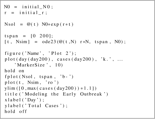
  Assuming you found a suitable combination of parameter values, you should see that the model does indeed track this portion of the data fairly well. However, so far we have only compared the model to the first 200 days. What about the rest of the data? The following code defines some new variables for selecting the first 300 days instead of the first 200 and regenerates the model on this extended set of points.

  

• (6) Generate a new plot that compares the model to the first 300 days of data. You can use the plotting code from exercise (5) as a template if needed. You may also change the number of days shown if desired (you could try stopping at 250 days or 400 days, for example).

• (7) You should see that the model does not work very well beyond 200 days. Describe any differences you see. What happens in the data as t becomes larger? What happens in the model as t becomes larger?

Model Development

Clearly we need to make some adjustments if we want our model to describe the full course of the outbreak. Let us look at the full dataset again to remind ourselves what the trend looks like.

The key difference appears to be that, while the number of cases in our model continues to accelerate as the number of days increases, the number of cases in the data begins to decelerate somewhere around 250 days and eventually stops changing much at all. So, we need to modify our model in a way that causes the rate of change in the number of cases to become small as the number of cases approaches some upper bound. Let us state this observation in a new differential equation:

$$\displaystyle \begin{aligned}dN / dt = r N * f(N, K)\end{aligned}$$

where f(N, K) represents some function of the number of cases and the upper bound that the data approaches—often this latter parameter is referred to as the carrying capacity. But what should the function f(N, K) look like? We would like f(N, K) to be close to 1 when the number of cases is small—that way, the value of r N will be close to what it was for our previous model, which worked pretty well when the number of cases was small. On the other hand, we want f(N, K) to be close to zero if the number of cases is getting close to the upper bound, K. That way, the rate of change will approach 0 as the number of cases increases, similar to our data. One form of f(N, K) that satisfies these properties is:

$$\displaystyle \begin{aligned}f(N, K) = 1 - N / K\end{aligned}$$

making our differential equation:

$$\displaystyle \begin{aligned}dN / dt = r N (1 - N / K)\end{aligned}$$

Before we go on, let us convince ourselves that this formula does in fact satisfy the properties we just mentioned.

Challenge Problem 4

• (8) What is the value of r N (1 - N / K) if N is small, say N = 0 ?

• (9) What is the value of r N (1 - N / K) if N is very close to K, say N = K ?

• (10) (Optional) Can you think of any other version of f(N, K) that might work? Try some out!

Testing the Model

Now that we are satisfied with the reasonableness of our new model, let us simulate it. This model also has a known expression for a solution, but we will proceed with simulation-only approach in order to prepare you for more complex cases. As before, we need to assign some initial guesses for our model’s parameter values. To prevent overwriting the variables we used before, we can name our new parameters n02, r2, etc. Fortunately, since our new model is very similar to the old model for certain portions of the data, the values we already determined for n0 and r should be decent guesses for n02 and r2.

This just leaves the parameter K.

Challenges

• (11) Use the data to make an initial guess for the value of the parameter K, then enter it in the code below. Recall that K represents the upper bound for the number of cases.

  

  After entering your answer, rerun the code for this section.

  Now we can compare the model to the data as before.

• (12) Run the code block below to plot the comparison. Then, enter new values for the parameters n02, r2, and K, and rerun the code block to see the new comparison. Try to find a combination of parameter values that makes the model and data match as closely as possible.

  

• (13) Would you say the model does a good job of describing the Ebola outbreak? Why or why not?

• (14) List one difference you notice between the data and the model.

• (15) Propose an explanation for the difference you noted in (14), in terms of the epidemic. You could also think of this in terms of what pieces the model might be missing.

5.3 Discussion

Back to our project-based challenges. The first attempt was to use the approximate proportional/exponential growth model based on early observations and try to predict the course of the disease. When you compare to the actual course, you will see that the model works well initially, but then drastically over-estimates the infections. That leads us to search for an alternative, and the logistic model provides a reasonable option. Once we have a reasonable model like the logistic growth model, we can try to assess key features of the outbreak process by analyzing the model itself. If you look at a result from Lab 3 that we show on Fig. 25, you will notice 2 things: first, the model matches observations reasonably well initially, but diverges significantly in later days. A logistic model cannot do much better than that, since it has some symmetries which the real data does not, so we will need to further revise the model to improve our prediction (Step 4 in Sect. 1.1).

Fig. 25

A graph of the WHO Ebola outbreak data (black dots) and a logistic model fit to it (red curve). We see that the model performs well initially, but has problems explaining the data later

Second, and perhaps more interesting, we see one prediction of the model that is mirrored in the data: the functions describing the total infected population size change their nature, from increasing initially, to decreasing in the later stages of the infection. We can translate that observation in mathematical statements, as per Step 2 in Sect. 1.1. In Calculus, such a transition from increasing to decreasing (or vice versa) happens at inflection points. Since this is obviously an important point to know for the epidemic, both the time at which it happens and the size of the infected population at that time, let us try to analyze the equation in order to find the inflection point. In principle, we can use the simulations in Lab 3, and you should try that, for some more ”computational thinking.” But we can also use analytical results based directly on the equation, without simulations or a known formula for a solution. One thing to note: when we have an expression about the derivative of a function, as in (22), we know a lot about the function itself. We know its first derivative, which means we can take a derivative and compute its second derivative. Then one more time, to obtain its third derivative, etc. So, basically, from the Eq. (22) we can find out ALL derivatives of R and only do not know the function itself, values for the population size R at specific times t!

Let us work out this analysis here. How can we find an inflection point of a function? Well, if the function transitions from increasing to decreasing, that means there is a minimum of the derivative of the function, so that the derivative is positive to the left of it (increasing) and negative to the right (decreasing). This means that an the inflection point the derivative of the derivative will be zero, which means that the second derivative of the solution is zero at an inflection point. Now that we have a feature to look for, we take the formula for the solution, find the second derivative, ... Oh, wait, we do not have the formula of the solution! However, we do have a formula for its derivative that was our model expressed as a differential equation (22)

$$\displaystyle \begin{aligned} R'(t) = k_0*\left(1-\frac{R(t)}{K}\right)*R(t) \end{aligned}$$

This is actually nice, since we do not have to compute the first derivative, we already know it. So if we take one more derivative of this equation, we will get

$$\displaystyle \begin{aligned}R''(t) = \frac{d}{dt}\left( k_0*\left(1-\frac{R(t)}{K}\right)*R(t)\right) \end{aligned}$$

Hmm, we have the second derivative, but the right hand side seems a bit messy. Do not we need R(t) after all? Let us persist, and evaluate the derivatives while keeping the unknown function R(t) and its derivative R′(t) as we come across them. Continuing with the product rule of the right hand side, we obtain

$$\displaystyle \begin{aligned}R''(t) = k_0*\left( -\frac{R'(t)}{K}*R(t) +\left(1-\frac{R(t)}{K}\right)*R'(t)\right) = k_0 *R'(t) \left( 1 -2 \frac{R(t)}{K} \right) \end{aligned}$$

That does not look too enlightening, until we remember that we do have an expression for R′(t)—that is the original equation (22). We substitute this expression for R′(t) on the right hand side to obtain

$$\displaystyle \begin{aligned} R''(t) = k_0 * k_0 * \left( 1 - \frac{R(t)}{K} \right)*R(t)* \left( 1 -2 \frac{R(t)}{K} \right) \end{aligned}$$

That equation is almost ready for analysis. For what values of R(t) would R″(t) be zero? From the right hand side, we see that R(t) = 0, K, or K∕2 are all possible solutions. However, R(t) = 0 and R(t) = K represent “no infection” and “everyone infected” states, respectively (known as fixed points), so we are left with the conclusion that the inflection point occurs when R(t) = K∕2, or half of the infectable population is infected. This analysis does not produce the time at which this inflection occurs: for that information, we would still need a formula or simulation. Try to find the time of inflection with a simulation in Lab 3. However, this approach does provide two useful predictions. First, it predicts a level of infection beyond which things would get better. Second, it predicts that, according to this model, it will take the same amount of time for things to get better as it took to get to that situation. Those are powerful and actionable predictions, and similar models have been used by WHO to respond to the Ebola, COVID, and other, epidemics.

6 Conclusions

In this chapter we presented a progression of biological situations, coupled by associated mathematical representations that reflect our understanding of these real-world situations. This is the gist of mathematical modeling. It is a process of discovery, and it is an iterative process, as summarized by Steps 1 through 4 in Sect. 1.1. The most important of them is probably Step 4 in Sect. 1.1, which asserts that anything we write down is not “the truth,” but just our latest, most improved understanding of the real-world situation that we are translating into a mathematical representation. We are using the term ”translate” quite literally here, since we think of mathematics as a language (or rather, a set of related languages), but a language which can provide much higher precision of expression compared to other human languages.

We as professional applied mathematicians are directly involved with using very similar models to approach and solve real-world problems. As noted previously, Prof. Guidoboni is currently directly involved in helping monitor hundreds of elderly individuals in over 10 long-care facilities. The predator-prey models discussed in Sect. 4 are not limited to model only behavior of predators and prey. They are also used in sociology and social psychology [20, 21]. Students of Dr. Dimitrov’s used a version of the Ebola modeling project as a stepping stone to identify and model problems from the current COVID pandemic and ultimately analyze different approaches to hospital utilization to help states manage the influx of COVID patients [29]. Should you chose to proceed on this path, soon you will be able to tackle difficult societal problems and help people on your own, through mathematical modeling.

We tried to demonstrate the breadth of situations that can be understood using mathematical models, while remaining within the domain of biological systems. Even that shows the breadth of problems that can be addressed mathematically, and the scope of results and conclusions that can be obtained in that way. You will hear this statement many times in your journey building and evaluating mathematical models, but it bears repeating: just start, summarize your thought in mathematical notation, and then let the math help you on the way.

References

G. Polya. How to solve it. Princeton University Press, 1945.
K. K. Bliss, F. K. Fowler, and B. J. Galluzzo. Math Modeling: Getting Started and Getting Solutions. SIAM, Philadelphia, 2014.
S. Buyting. Women and science suffer when medical research doesn’t study females. https://www.cbc.ca/radio/quirks/july-25-2020-women-in-science-special-how-science-has-done-women-wrong-1.5291077/women-and-science-suffer-when-medical-research-doesn-t-study-females-1.5291080, 2019. Accessed: 2021-02-07.
Code files for the chapter. https://github.com/adimitr/ModelingBioChapter. Accessed: 2021-06-30.
Matlab:. https://www.mathworks.com/products/matlab.html. Accessed: 2021-01-30.
GNU Octave:. https://www.gnu.org/software/octave/index. Accessed: 2021-01-30.
Python:. https://www.python.org/. Accessed: 2021-01-31.
Jupyter notebook:. https://jupyter.org/. Accessed: 2021-01-31.
Matlab onramp:. https://www.mathworks.com/learn/tutorials/matlab-onramp.html. Accessed: 2021-01-31.
Octave tutorials:. https://wiki.octave.org/Video_tutorials. Accessed: 2021-01-31.
S Freeman, SL Eddy, M McDonough, M Smith, N Okoroafora, H Jordt, and MP Wenderoth. Active learning increases student performance in science, engineering, and mathematics. Proceedings of the National Academy of Sciences, 11(3):8410–8415, 2014.
I Starr and A Noordergraaf. Ballistocardiography in cardiovascular research: Physical aspects of the circulation in health and disease. Lippincott, 1967.
G Guidoboni, L Sala, M Enayati, R Sacco, M Szopos, J Keller, M Popescu, L Despins, V Huxley, and M Skubic. Cardiovascular function and ballistocardiogram: a relationship interpreted via mathematical modeling. IEEE Transactions on Biomedical Engineering, 66(10):2906–2917, 2019.
D Kincaid and W Cheney. Numerical Analysis: Mathematics of Scientific Computing. American Mathematical Society, 2002.
JR Hanly and EB Koffman. Problem solving and program design in C. Pearson, New Jersey, 2018.
DN Arnold. The patriot missile failure. http://www-users.math.umn.edu/~arnold//disasters/patriot.html, 2000. Accessed: 2021-02-02.
RB Schmid, A Knutson, KL Giles, and BP Mcornack. Hessian fly (Diptera: Cecidomyiidae) biology and management in wheat. Journal of Integrated Pest Management, 9(1), 2018.
Roe K. Tolerance as a novel mechanism of hessian fly control on wheat. Master’s thesis, Purdue University, 2016.
CM Packard. Life histories and methods of rearing hessian-fly parasites. Journal of Agricultural Research, 6(10):367–381, 1916.
P Oliver and D Myers. The coevolution of social movements. Mobilization, 8:1–25, 2003.
D Felmlee and D Greenberg. A dynamic systems model of dyadic interaction. Journal of Mathematical Sociology, 23(3):155–180, 1999.
SIMIODE modeling scenarios. https://www.simiode.org/resources/modelingscenarios. Accessed: 2021-01-30.
T.R. Malthus. An Essay on the Principle of Population As It Affects the Future Improvement of Society, with Remarks on the Speculations of Mr. Goodwin, M. Condorcet and Other Writers. J. Johnson in St. Paul’s Churchyard, London, 1798. https://archive.org/details/essayonprincipl00malt, Accessed: 2021-01-30.
P.-F. Verhulst. Recherches mathématiques sur la loi d’accroissement de la population. Nouveaux Mémoires de l’Académie Royale des Sciences et Belles-Lettres de Bruxelles, 18:1 – 38, 1845.
McKendrick A. G. and Pai M. K. XLV.—the rate of multiplication of micro-organisms: A mathematical study. Proceedings of the Royal Society of Edinburgh, 31:649 – 653, 1912.
World Health Organization. Ebola virus disease. http://www.who.int/mediacentre/factsheets/fs103/en/. Accessed: 2021-02-05.
The covid tracking project:. https://covidtracking.com/. Accessed: 2021-02-05.
Ensheng Dong, Hongru Du, and Lauren Gardner. An interactive web-based dashboard to track covid-19 in real time. The Lancet Infectious Diseases, 20:533–534, 5 2020.
M. D. Roberts, H. D. Seymour, and A. Dimitrov. Increasing number of hospital beds has inconsistent effects on delaying bed shortages due to COVID-19. SIAM Undergraduate Research Online, 2021.
Author information
Authors and Affiliations
Corresponding author
Editor information
Editors and Affiliations
Rights and permissions
Copyright information
© 2022 The Author(s), under exclusive license to Springer Nature Switzerland AG
About this chapter
Cite this chapter
Dimitrov, A. et al. (2022). Modeling of Biological Systems: From Algebra to Calculus and Computer Simulations. In: Goldwyn, E.E., Ganzell, S., Wootton, A. (eds) Mathematics Research for the Beginning Student, Volume 1. Foundations for Undergraduate Research in Mathematics. Birkhäuser, Cham. https://doi.org/10.1007/978-3-031-08560-4_7
Download citation
DOI: https://doi.org/10.1007/978-3-031-08560-4_7
Published:
Publisher Name: Birkhäuser, Cham
Print ISBN: 978-3-031-08559-8
Online ISBN: 978-3-031-08560-4
eBook Packages: Mathematics and StatisticsMathematics and Statistics (R0)