
Abstract
A suite of related online and offline analysis and visualisation tools for training students of phonetics in the acoustics of prosody is described in detail. Prosody is informally understood as the rhythms and melodies of speech, whether relating to words, sentences, or longer stretches of discourse, including dialogue. The aim is to contribute towards bridging the epistemological gap between phonological analysis, based on the linguist’s intuition together with structural models, on the one hand, and, on the other hand, phonetic analysis based on measurements and physical models of the production, transmission (acoustic) and perception phases of the speech chain. The toolkit described in the present contribution applies to the acoustic domain, with analysis of the low frequency (LF) amplitude modulation (AM) and frequency modulation (FM) of speech, with spectral analyses of the demodulated amplitude and frequency envelopes, in each case as LF spectrum and LF spectrogram. Clustering functions permit comparison of utterances.
Access provided by Autonomous University of Puebla. Download conference paper PDF
Keywords
1 Introduction
A suite of related online and standalone analysis and visualisation tools for training students of phonetics in the acoustics of prosody is described. Prosody is informally understood as the rhythms and melodies of speech, whether relating to words, sentences, or longer stretches of discourse, including dialogue. The aim is to contribute towards the epistemological gap between phonological analysis of prosody, based on the linguist’s qualitative intuition, hermeneutic methods and structural models on the one hand, and, on the other, the phonetic analysis of prosody based on quantitative measurements, statistical methods and causal physical models of the production, transmission (acoustic) and perception phases of the speech chain. The phonetician’s methodology also starts with intuitions, even if only to distinguish speech from other sounds, or more specifically to provide categorial explicanda for quantitatively classifying the temporal events of speech. Nevertheless, the two disciplines rapidly diverge as the domains and methods become more complex, and issues of the empirical grounding of phonological categories beyond hermeneutic intuition arise. The present contribution addresses two of these issues:
-
1.
models of rhythm as structural patterns which correspond to intuitions of stronger and weaker syllables and words in sequence;
-
2.
intuitive perception of globally rising and falling pitch contours.
The present account focusses exclusively on the acoustic phonetics of speech transmission, not on production or perception, with a tutorial method of data visualisation in two main prosodic domains:
-
1.
LF (low frequency) amplitude modulation (AM) of speech as phonetic correlates of sonority curves covering the time-varying prominences of syllables, phrases, words and larger units of discourse as contributors to speech rhythms;
-
2.
LF frequency modulation (FM) of speech as the main contributor to tones, pitch accents and stress-pitch accents, to intonations at phrasal and higher ranks of discourse patterning, and also as a contributor to speech rhythms.
In Sect. 2, components of the online tool are described, centring on the demodulation of LF AM and FM speech properties. In Sect. 3 an open source extended offline toolkit for Rhythm Formant Analysis (RFA) procedure is described, followed by a demonstration of the RFA tool in a comparison of readings of translations of a narrative into the two languages of a bilingual speaker. Finally, conclusions are discussed in Sect. 4.
2 An Online Tool: CRAFT
2.1 Motivation
The motivation for the CRAFT (Creation and Recovery of Amplitude and Frequency Tracks) online speech analysis tutorial tool and its underlying principles are described, together with some applications, in [9] and [12]. Well-known tools such as Praat [3], WinPitch [19], AnnotationPro [18], ProsodyPro [29] and WaveSurfer [22] are essentially dedicated offline research tools. The online CRAFT visualisation application is a tutorial supplement to such tools, based on the need to develop a critical and informed initial understanding of strengths and weaknesses of different algorithms for acoustic prosody analysis. The main functional specifications for this online tool are: accessibility, version-consistency, ease of maintenance, suitability for distance tutoring, face-to-face teaching and individual study, and also interoperability using browsers on laptops, tablets and (with size restrictions) smartphones.
CRAFT is implemented in functional programming style using Python3 and the libraries NumPy, SciPy and MatPlotLib, with input via a script-free HTML page with frames (sometimes deprecated, but useful in this context), server-side CGI processing and HTML output. The graphical user interface (GUI) has one output frame and four frames for different input typesFootnote 1 (Fig. 1):
-
1.
study of selected published F0 estimators (Praat, RAPT, Reaper, SWIPE, YAAPT, Yin) and F0 estimators custom-designed for CRAFT (AMDF or Average Magnitude Difference Function, and S0FT, Simple F0 Tracker);
-
2.
visualisation of amplitude and frequency modulation and demodulation operations;
-
3.
display of alternative time and frequency domain based FM demodulation (F0 estimation, ‘pitch’ tracking);
-
4.
visualisation of low-pass, high-pass and band-pass filters, Hann and Hamming windows, Fourier and Hilbert transformations;
-
5.
visualisation of the output generated by the selected input frame.

CRAFT GUI: parameter input frame (top) for 9 F0 extractor algorithms; amplitude demodulation (left upper mid); F0 estimators (left lower mid); filters, transforms, spectrogram (left bottom); output frame (lower right).
In the following subsections, LF AM and LF FM visualisations are discussed, followed by descriptions of AM and FM demodulation, operations and transforms and long-term spectral analysis.
2.2 Amplitude Modulation (AM) and Frequency Modulation (FM)
The mindset behind the CRAFT tool is modulation theory (cf. also [28]): in the transmission of speech signals a carrier signal is modulated by an information-bearing lower frequency modulation signal, and in perception the modulated signal is demodulated to extract the information-bearing signal; cf. Fig. 2. Two main types of modulation are provided in the speech signal: amplitude modulation and frequency modulation. Both these concepts are familiar from the audio modulation of HF and VHF broadcast radio with amplitude modulation between about 100 kHz and 30 MHz (AM radio), and frequency modulation between about 100 MHz and 110 MHz (FM radio). The top frame in Fig. 1 provides inputs and parameters for the two core CRAFT tasks, exploring two prosodic subdomains: properties of F0 estimation algorithms and long term spectral analysis of demodulated amplitude and frequency envelopes. Corpus snippets are provided, including The North Wind and the Sun read aloud in English and in Mandarin.

AM and FM panels (top to bottom): modulation signal, carrier signal, amplitude modulated carrier, amplitude modulation spectrum, demodulated AM signal (rectification, peak-picking or Hilbert); frequency modulated carrier, frequency modulation spectrum, demodulated FM signal.
Alternating sequences of consonant clusters (lower amplitude) and vowels (higher amplitude) provide a low frequency (LF) AM sonority cycle of syllable sequences. The syllable lengths and corresponding modulation frequencies are around 100 ms (10 Hz) and 250 ms (4 Hz), and there are longer term, lower frequency amplitude modulations corresponding roughly to phrases, sentences and longer units of speech, constituting the LF formants of speech rhythms. Consonant-vowel sequences also involve a more complex kind of amplitude modulation: variable filtering of the amplitude of the high frequency (HF) harmonics of the fundamental frequency (and consonant noise filtering), creating the HF formants which distinguish speech sounds.
The CRAFT tool is designed for analysis of the LF rhythm formants which correlate with long-term LF AM sequences of syllables and of larger linguistic units, not for the analysis of HF formants. Global falling, rising or complex intonation patterns and local lexical tones, pitch accents or stress-pitch accents underlie the FM patterns of speech. The CRAFT input form for visualisation of amplitude and frequency modulation and demodulation procedures is shown in Fig. 3.

Parameter input for AM and FM module.
2.3 Amplitude and Frequency Demodulation
Amplitude demodulation is implemented as the outline of the waveform of the signal, the positive envelope of the signal, created by means of the smoothed (low-pass filtered) absolute Hilbert transform, peak picking on the smoothed signal, or rectification and smoothing of the signal. Frequency demodulation is implemented as F0 estimation (‘pitch’ tracking) of the voiced segments of the speech signal.
Frequency demodulation of speech signals differs from the frequency demodulation of FM radio signals in various ways, though the principle is the same. The FM radio signal varies around a continuous, stable and well-defined central carrier frequency, with frequency changes depending on the amplitude changes of the modulating audio signal, and when the modulation is switched off the carrier signal remains as a reference signal. But in frequency demodulation of a speech signal there is no well-defined central frequency, the signal is discontinuous (in voiceless consonants and in pauses), the frequency cycles are uneven, since the vocal cords are soft and moist (and not mechanically or mathematically precisely defined oscillators), and when the modulation disappears, so does the fundamental frequency carrier signal – there is no unmodulated carrier; cf. [28]. For these reasons, in order to demodulate the speech fundamental frequency, the signal has to undergo a range of transformations.
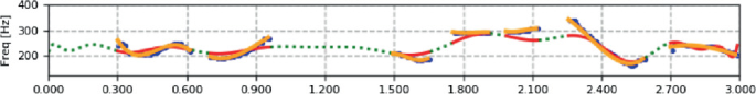
Several comparisons and analyses of techniques for frequency demodulation (F0 estimation) of the speech signal are discussed in [1, 15, 17, 20] are facilitated. The following ten panels show visualisations of F0 estimates by a selection of algorithms, each selected and generated separately using CRAFT, with the same data. The algorithms produce similar results, though there are small local and global differences. The superimposed polynomial functions illustrate some non-obvious differences between the estimates: a local polynomial model for voiced signal segments and a global model for the entire contour with dotted lines interpolating across voiceless segments are provided.
-
1.
Average Magnitude Difference Function (AMDF; custom implementation)

-
2.
Praat (autocorrelation) [3]

-
3.
Praat (cross-correlation) [3]

-
4.
RAPT [23]

-
5.
PyRAPT (Python emulation) [8]

-
6.
Reaper [24]

-
7.
S0FT (custom implementation)
-
8.
SWIPE (Python emulation) [4, 7]

-
9.
YAAPT (Python emulation) [21, 30]

-
10.
YIN (Python emulation) [6, 13]


The F0 estimations in Panels 1 to 10 are applications of the different algorithms to the same data with default settings. Two polynomial models are superimposed in each case. The colour coding is: F0: blue, local polynomial: orange, global polynomial: red plus dotted green interpolation. The algorithms achieve quite similar results and correlate well (cf. Table 1), and are very useful for informal ‘eyeballing’. Most of the algorithms use time domain autocorrelation or cross-correlation, while the others use frequency domain spectrum analysis or combinations of these techniques. CRAFT provides basic parametrisation for all the algorithms as follows:
-
start and length of signal (in seconds),
-
F0min and F0max for frequency analysis and display,
-
length of frame for F0 analysis,
-
length of median F0 smoothing filter,
-
orders of global and local F0 polynomial model,
-
on/off switch for F0 display,
-
spectrum min and max frequencies,
-
display min and max for envelope spectrum,
-
power value for AM and FM difference spectra,
-
display width and height.
AMDF and S0FT are minimalistic implementations which were designed specifically for the CRAFT tool. Except for a couple of sub-octave errors in the default configuration shown, AMDF compares favourably with Praat autocorrelation, which it resembles, except for the use of subtraction and not multiplication, resulting in a faster algorithm. Absolute speed is dependent on the implementation environment, of course, with C or C++ being in principle faster than Python. Interestingly, the Python YIN implementation is the fastest of all.
The S0FT F0 estimation algorithm has a different purpose from the others: parameters for ‘tweaking’ of the analysis are provided in order to find an optimal agreement with aural-visual inspection and accepted standard algorithms. In addition to the general parameters for adjustment by the user, which are available to all algorithms, S0FT also provides specific parameters:
-
initial choice:
-
voice type (higher, middle, lower pitch), or
-
custom: levels of centre-clipping, high and low pass,
-
-
if initial choice is custom:
-
filter frequency and order,
-
algorithm (FFT, zero-crossing, peak-picking),
-
length of F0 median filter,
-
min and max y-axis display clipping.
-
An example of S0FT output is shown in Panel 7 above. With the parameter defaults provided, the results can be very close to the output of standard algorithms such as the autocorrelation algorithm of Praat.
The quantitative measurements which underlie the visualisations are also available for further use, as in Table 1, which shows correlations between the algorithms under the same conditions and for a single data item (bearing in mind that the goal here is not to report an experiment but to outline the potential of this online tool).
2.4 Operations and Transforms
CRAFT also includes a panel for illustrating low-pass, high-pass and band-pass filters, Hann (cosine; also, correctly: von Hann, and incorrectly: ‘Hanning’), and Hamming (raised cosine) windows, as well as Fourier and Hilbert Transforms and a parametrised spectrogram display. The following three panels show low-pass, high-pass and band-pass filters and the von Hann window.
-
1.
High-pass and low-pass filters.

-
2.
Band-pass filter with illustration of application.

-
3.
von Hann window with illustration of application.


Figure 4 shows Fast Fourier Transforms (FFT) of six frequency estimations. Clearly the F0 spectra of these algorithms differ considerably in spite of the rather high correlations noted previously, because of differences in frequency vs. time domain processing, in window lengths and window skip distances, as well as in internal filtering. S0FT, AMDF and PyRAPT are rather similar, while YAAPT, Praat (cross-correlation) and SWIPE are very different. The implication is that when demodulated F0 is further processed quantitatively, these differences between the algorithms may need to be taken into account, in spite of the relatively high correlations between them.

Spectral analysis 0…20 Hz of frequency envelopes of selected F0 estimation algorithms for the same signal: S0FT, YAAPT, Praat (cross-correlation), AMDF, PyRAPT, SWIPE (top to bottom, left column before right).
3 The RFA Offline Extension Toolkit
3.1 Functional Specification
The main aim of the RFA (Rhythm Formant Analysis) toolkit extension is detailed investigation of the contributions of LF AM and LF FM to the analysis of speech rhythms, based on the concept of rhythm formant, that is, a region of high magnitudes in the low frequency spectrum and spectrogram of the speech signal, relating to the rhythms of words and syllables, and, in long utterances, to slower rhythms of phrases and longer discourse units. Theoretical foundations of the underlying Rhythm Formant Theory (RFT) and applications of the RFA toolkit are described in [12]. The code is available on GitHub (https://github.com/dafyddg/RFA).
Intuitively, rhythm is understood to be a real-time sequence of regular acoustic beats, usually between one and four per seconds (1…4 Hz). These beats are often said to be associated with stressed syllables in foot-based stress-pitch accent languages like English, and with each syllable in syllable-based languages like Chinese.
There are many approaches to the analysis of speech rhythms in linguistics and phonetics. Phonological approaches use numerical values, or tree structures with nodes labelled ‘strong’ and ‘weak’, or bar-chart like ‘grids’ to visualise a qualitative abstract notion of intuitively identified rhythm. Descriptive phonetic approaches annotate speech recordings with boundaries of intervals associated with phonological categories such as vocalic, consonantal, syllable or word segments and use strategies to form averages of interval duration differences and to apply the averages as indices for characterising language types.
A major issue with the annotation based duration average approaches is the lack of phonetic grounding in the reality of speech signals beyond crude segmentation. The reality of rhythm is that it involves more than just duration averages: it involves oscillations in real time of beats and waves with approximately equal intervals – relative or ‘fuzzy’ isochrony. The restrictive duration average methods have failed to find isochrony, for a number of simple reasons which have been discussed on many occasions; cf. the summary in [12]. In particular, the duration average methods do not actually capture the rhythms of speech, because they…
-
1.
ignore the ‘beat’ or oscillation property of speech rhythms;
-
2.
assume constant duration patterning throughout utterances;
-
3.
assume a single duration average for each language.
In fact, rhythms may hold over quite short subsequences of three or more beats and then change in frequency, also on occasion in a longer term rhythmic pattern, the ‘rhythms of rhythm’ [12]. Further, rhythms vary not only from language to language and dialect to dialect, but also with different pragmatic speech styles.
Parallel to and in stark contrast with the annotation based duration average approaches are the signal processing approaches which start with the assumption of rhythm as oscillating signal modulations, and work with spectral analysis and related transformations to discover speech rhythms of different frequencies below about 10 Hz; cf. overviews in [9, 12] and Sect. 2.3, For example, a syllable speech rate of 5 syll/s corresponds to a low oscillation frequency of 5 Hz with an average syllable length of 0.2 s; a foot speech rate of 1.5 ft/s corresponds to an oscillation frequency of 1.5 Hz and average foot length of 0.6 s. The prediction is that with an appropriate spectral analysis, these and other rhythm frequencies can be detected inductively from the speech signal. Correspondingly, the intuitive understanding of ‘rhythm’ is explicated ‘bottom-up’, unlike top-down phonological approaches, starting with the intuition of rhythm as oscillation and then analysing physical properties of the speech signal, based on the modulation theoretic perspective of signal processing (Gibbon 2021:3):
Speech rhythms are fairly regular oscillations below about 10 Hz which modulate the speech source carrier signal and are detectable in spectral analysis as magnitude peaks in the LF spectrum of both the amplitude modulation (AM) envelope of the speech signal, related to the syllable sonority outline of the waveform, and the frequency modulation (FM) envelope of the signal, related to perceived pitch contours.
The central requirement for a tool to be used for identifying rhythm frequencies by demodulation of the low frequency oscillating modulations of the speech signal is thus the identification of temporally regular oscillations with specific frequencies or, more realistically, frequency ranges. The frequency zones define multiple fuzzy-edged rhythm formants (cf. [9,10,11,12]), which can be associated with signal modulations by syllables, phrases and other categories [2, 5, 16]. In other words: the tool must include a method for demodulating the rhythmically modulated signal.
For this purpose, long-term spectrogram analysis of the positive signal amplitude envelope is introduced, both to analyse rhythms quantitatively, and to model the perception of varying rhythms in the LF AM and FM oscillations of speech signals (cf. [14, 25,26,27]).
The full procedure of demodulation and spectral analysis is shown with a stylised example in Fig. 5. In the example, the signal length is 1 s, the sampling frequency is 44.1 kHz, the modulation frequency is 10 Hz and the modulation index (modulation depth) is 0.75.

Panels showing simplified aspects of amplitude modulation, demodulation and rhythm detection: 1. sine modulation wave, 2. sine carrier wave, 3. modulated carrier, 4. demodulated amplitude envelope, 5. amplitude envelope spectrum.
3.2 Standalone Offline Tools
Online tools are useful for teaching demonstrations in teaching situations where the user is a software consumer rather than developer, but have the disadvantage that they are constrained by the designer’s goals and the further disadvantages of software and data integrity and possibly also unwanted logging of interactive activities.
For more flexibility, though at the cost of ease of use, a companion set of standalone offline tools was developed, also using Python3 and the libraries NumPy, SciPy, MatPlotLib, plus GraphViz. The toolset provides:
-
1.
analysis and visualisation of AM and FM demodulation;
-
2.
low frequency spectral analysis of AM and FM;
-
3.
both a global spectrum and a 2 s or 3 s long windowed spectrogram for entire utterances;
-
4.
trajectories of highest magnitude frequencies through the spectrogram frame series;
-
5.
comparison of utterances using these criteria.
The goal here is not to produce off-the-shelf point-and-click consumer software, but to produce a suite of basic ‘alpha standard’ command-line tool prototypes which can be further developed by the interested user.
Figure 6 (upper left) shows the waveform (grey) and the rectified and low pass filtered amplitude envelope (red). The low pass filtered long-term amplitude envelope is taken to be the acoustic phonetic correlate of the ‘sonority curve’ of phonological analyses. The LF spectrum from 0 Hz to 5 Hz is shown in Fig. 6 (upper right); groups of high magnitude frequencies are taken to represent rhythm formants at different frequcies, the correlates of superordination and subordination prosodic hierarchy patterns in the locutionary component of the utterance. FM demodulation and spectral analysis are analogous.

Rhythm frequency identification procedure.
In the mid panels of Fig. 6, spectrograms of the utterance are shown, extracted in 2 ms overlapping FFT windows, first visualised as a waterfall spectrum, from top to bottom, consisting of a vertical sequence of spectra in the frequency domain (mid right), and also as a more conventional heatmap spectrogram in the time domain (mid left), with higher magnitudes shown as darker colours.
The main innovations in the offline toolkit are:
-
1.
the LF spectrogram, which permits the observation and further analysis of changes in rhythm patterns through the utterance;
-
2.
the extraction of a trajectory through the spectrogram, in which at every FFT analysis window the frequency with the highest magnitude is selected;
-
3.
the custom design of the AMDF FM demodulation algorithm, in which frame duration and correlation domain are adjusted automatically in terms of minimum and maximum limit parameters for the frequency search space;
-
4.
clustering procedures for comparing sets of utterances:
-
prosodic k-means clustering;
-
prosodic distance mapping of utterances with a selection of distance metrics;
-
prosodic hierarchical clustering with selections of distance metric and clustering condition combinations.
-
In order to be able to combine these functions in different ways for different purposes, for example only the waveform, or with the AM envelope and the FM track (F0 estimation track), with the low frequency AM and FM spectra, or only the waveform, F0 estimation, AM LF spectrogram and FM LF spectrogram, a set of libraries was developed for specific analysis tasks:
-
1.
waveform and LF amplitude demodulation (in the main application);
-
2.
module_fm_demodulation.py (LF FM, LF F0 estimation, using a custom variant of AMDF, the Average Magnitude Difference Function);
-
3.
module_drawdendrogram.py (spectral frequency grouping of magnitude peaks interpreted as rhythm formants);
-
4.
module_spectrogram.py (LF spectrogram of utterance, typically with 2s or 3s LF FFT window);
-
5.
module_kmeans.py (classification of sets of utterances using Euclidean distance-based k-means clustering);
-
6.
module_distancenetworks.py (distance-based linking of utterances according to time domain and frequency domain spectrum and spectrogram data vectors, using a selection of distance metrics: Canberra, Chebyshev, Cosine, Euclidean, Manhattan);
-
7.
module_hierarchicalclustering.py (hierarchical clustering based on a selection of distance metrics and clustering conditions).
3.3 Prosodic Comparison of Narrative Readings
For demonstration purposes an analysis of spoken narrative data was conducted on a small data set of readings aloud of the IPA benchmark narrative The North Wind and the Sun in English and German by a female bilingual speaker. The readings in each language are numbered in order of production; the German readings were produced before the English readings. While rhythms of spontaneous speech and dialogue may appear more interesting at first glance, reading aloud is a cultural technique with independent inherent value in report presentation, news-reading or reading to children and the sight-afflicted. Moreover, spontaneous more complex and it is advisable to introduce a new method with simpler clear cases.
As the first basic step, k-means analysis was chosen. The analysis is intended to demonstrate the value of both time and frequency domain parameters in prosodic typology. The prediction is that the readings in English and German can be distinguished by means of selected prosodic parameters, even though the readings are by the same speaker.
There are many prosodic properties which can be addressed. The present analysis uses variance in two time domain vectors:
-
1.
x: the variance of the trajectory of the highest magnitude frequencies in the LF spectrogram;
-
2.
y: the variance of the FM (F0) track.
The two measures ignore the facts that (a) the data set is tiny and (b) the parameters concerned are locally and globally varying time functions, not static populations, thus not being ideal candidates for variance analysis. However, with durations of approximately 60 s the utterances are much longer than the domains of rhythmic variation such as syllable, word and phrase, so that ‘the end justifies the means’ in this case. The readings in English cluster in the upper right quadrant, while the readings in German cluster in the lower left quadrant; cf. Fig. 7. The result shows that the bilingual speaker makes a clear distinction between her readings in English and her readings in German In Fig. 7, data positions are marked with filled circles coloured by cluster; centroid positions are marked with “C” in a square in the cluster colour.

k-means positioning of readings of The North Wind and the Sun by AM and FM spectral properties.
3.4 Distance Mapping
Other similarity visualisations such as distance maps show links which are compatible with the k-means division. In order to make distance relations clearer at a glance, distances above 0.75 (range 0…1) were excluded from the graph.
The first analysis compares utterances on the basis of the LF AM spectrum vectors (Fig. 8), using the Cosine Distance metric. The readings in English are nearer to each other than to the readings in German, and vice-versa, with cluster-internal distances <0.7 in each case. However the first reading in English is nearer to the first reading in German than to the last reading in English, perhaps due to the chronology of the scenario: the last reading in German was produced immediately before the first reading in English. Such ordering effects were intended, as systematic context.

AM LF spectrum distances (English and German readings by female bilingual).

FM LF spectrogram frequency max peak distances (English and German readings by female bilingual).
The second analysis (Fig. 9) compares utterances on the basis of the LF FM spectrum vectors. The analysis also uses the Cosine Distance metric, and shows the same cluster formation as the analysis based on LF AM spectrum vectors: the readings in English are nearer to each other than to the readings in German, here with cluster-internal distances <0.6 in each case.. In this case, the first reading in English is nearer to both the first and third readings in German than to the third reading in English.
Further analyses based on spectrogram properties rather than spectrum properties, also conducted with the Cosine Distance metric, show the same clear partitions and also similar anomalies. The results are also confirmed by further analysis with hierarchical clustering (cf. Gibbon 2021).
4 Conclusion
The functionality of the CRAFT online tutorial tool and the extended offline RFA toolkit for acoustic prosody analysis is demonstrated in some detail, with attention to the rhythmic and melodic modulations of speech. The main uses of the toolkits are in advanced phonetics teaching and in acoustic prosody research. Many open research questions (cf. the discussion in [12]) can be addressed using the toolkits, such as the quantitative analysis of the variability of speech rhythms in different language domains, from varying rhythms of the consonant vowel succession in syllables (in so-called ‘syllable-timed languages’), to varying rhythms of syllable sequences in feet (in so-called ‘pitch accent languages’) and the much longer domains of rhythms in discourse.
Evidently, the small data set does not permit wide-ranging predictions. For larger data sets more sophisticated methods and complementing of the present strategy of unsupervised machine learning (ML) by semi-supervised and supervised ML methods. will be needed. However, the data set fulfils its function of demonstrating the validity of the RFA method itself and the utility of the extended RFA toolkit, and the heuristic value of the method in raising further pertinent questions is clear.
Notes
- 1.
http://wwwhomes.uni-bielefeld.de/gibbon/CRAFT/; code accessible on GitHub.
References
Arjmandi, M.K., Dilley, L.C., Lehet, M.: A comprehensive framework for F0 estimation and sampling in modeling prosodic variation in infant-directed speech. In: Proceedings of the 6th International Symposium on Tonal Aspects of Language, Berlin, Germany (2018)
Barbosa, P.A.: Explaining cross-linguistic rhythmic variability via a coupled-oscillator model of rhythm production. Speech Prosody 2002, 163–166 (2002)
Boersma, P.: Praat, a system for doing phonetics by computer. Glot Int. 5(9/10), 341–345 (2001)
Camacho, A.: SWIPE: A Sawtooth Waveform Inspired Pitch Estimator for Speech and Music. Ph.D. thesis, University of Florida (2007)
Cummins, F., Port, R.: Rhythmic constraints on stress timing in English. J. Phon. 1998(26), 145–171 (1998)
De Cheveigné, A., Kawahara, H.: YIN, a fundamental frequency estimator for speech and music. J. Acoust. Soc. Am. 111(4), 1917–1930 (2002)
Garg, D.: SWIPE pitch estimator (2018). https://github.com/dishagarg/SWIPE. [PySWIPE]
Gaspari, D.: Mandarin Tone Trainer. Master’s thesis, Harvard Extension School (2016). https://github.com/dgaspari/pyrapt
Gibbon, D.: The future of prosody: It’s about time. Proc. Speech Prosody 9 (2018). https://www.isca-speech.org/archive/SpeechProsody_2018/pdfs/_Inv-1.pdf
Gibbon, D.: Rhythm zone theory: speech rhythms are physical after all. In: Wrembel, M., Kiełkiewicz-Janowiak, A., Gąsiorowski, P. (eds.) Approaches to the Study of Sound Structure and Speech. Interdisciplinary Work in Honour of Katarzyna Dziubalska-Kołaczyk. Routledge, London (2019). https://arxiv.org/abs/1902.01267
Gibbon, D.: CRAFT: A Multifunction Online Platform for Speech Prosody Visualisation (2019). https://arxiv.org/pdf/1903.08718.pdf
Gibbon, D.: The rhythms of rhythm. J. Int. Phonetic Assoc. First View 1–33 (2021). https://doi.org/10.1017/S0025100321000086
Guyot, P.: Fast Python implementation of the Yin algorithm (2018). https://github.com/patriceguyot/Yin/
Hermansky, H.: History of modulation spectrum in ASR. In: Proceedings of the ICASSP 2010 (2010)
Hess, W.: Pitch Determination of Speech Signals: Algorithms and Devices. Springer, Berlin (1983). https://doi.org/10.1007/978-3-642-81926-1
Inden, B., Malisz, Z., Wagner, P., Wachsmuth, I.: Rapid entrainment to spontaneous speech: a comparison of oscillator models. In: Miyake, N., Peebles, D., Cooper, R.P. (eds.) Proceedings of the 34th Annual Conference of the Cognitive Science Society. Cognitive Science Society, Austin (2012)
Jouvet, D., Laprie, Y.: Performance analysis of several pitch detection algorithms on simulated and real noisy speech data. In: 25th European Signal Processing Conference (2017)
Klessa, K.: Annotation Pro. Enhancing Analyses of Linguistic and Paralinguistic Features in Speech. Wydział Neofilologii UAM, Poznań (2016)
Martin, P.: WinPitch: un logiciel d’analyse temps réel de la fréquence fondamentale fonctionnant sous Windows. Actes des XXIV Journées d’Étude sur la Parole, Avignon 224–227 (1996)
Rabiner, L.R., Cheng, M.J., Rosenberg, A.E., McGonegal, C.A.: A comparative performance study of several pitch detection algorithms. IEEE Trans. Acoust. Speech Sig. Process. ASSP-24(5), 399–418 (1976)
Schmitt, B.J.B.: AMFM_decompy (2014). [PyYAAPT]. https://github.com/bjbschmitt/AMFM_decompy
Sjölander, K., Beskow, J.: Wavesurfer – an open source speech tool. Proc. Interspeech 464–467 (2000). http://www.speech.kth.se/wavesurfer/
Talkin, D.: A robust algorithm for pitch tracking (RAPT). In: Kleijn, W.B., Palatal, K.K. (eds.) Speech Coding and Synthesis, pp. 497–518. Elsevier Science B.V. (1995)
Talkin, D.: Reaper: Robust Epoch And Pitch EstimatoR (2014). https://github.com/google/REAPER
Tilsen, S., Johnson, K.: Low-frequency Fourier analysis of speech rhythm. J. Acoust. Soc. Am. 124(2), EL34–EL39 (2008). [PubMed: 18681499]
Tilsen, S., Arvaniti, A.: Speech rhythm analysis with decomposition of the amplitude envelope: characterizing rhythmic patterns within and across languages. J. Acoust. Soc. Am. 134, 628 (2013)
Todd, N.P.M., Brown, G.J.: A computational model of prosody perception. ICSLP 94, 127–130 (1994)
Traunmüller, H.: Conventional, biological, and environmental factors in speech communication: a modulation theory. In Dufberg, M., Engstrand, O. (eds.) PERILUS XVIII: Experiments in Speech Process, pp. 1–19. Department of Linguistics, Stockholm University, Stockholm (1994). [Also in Phonetica 51, 170–183 (1994)]
Xu, Y.: ProsodyPro – a tool for large-scale systematic prosody analysis. In: Tools and Resources for the Analysis of Speech Prosody (TRASP 2013), Aix-en-Provence, France, pp. 7–10 (2013)
Zahorian, S.A., Hu, H.: A spectral/temporal method for robust fundamental frequency tracking. J. Acoust. Soc. Am. 123(6), 4559–4571 (2008). [YAAPT]
Author information
Authors and Affiliations
Corresponding author
Editor information
Editors and Affiliations
Rights and permissions
Copyright information
© 2022 Springer Nature Switzerland AG
About this paper

Cite this paper
Gibbon, D. (2022). The Phonetic Grounding of Prosody: Analysis and Visualisation Tools. In: Vetulani, Z., Paroubek, P., Kubis, M. (eds) Human Language Technology. Challenges for Computer Science and Linguistics. LTC 2019. Lecture Notes in Computer Science(), vol 13212. Springer, Cham. https://doi.org/10.1007/978-3-031-05328-3_3
Download citation
DOI: https://doi.org/10.1007/978-3-031-05328-3_3
Published:
Publisher Name: Springer, Cham
Print ISBN: 978-3-031-05327-6
Online ISBN: 978-3-031-05328-3
eBook Packages: Computer ScienceComputer Science (R0)