Structural Analysis and Optimization of Fixation Devices Used in Treatment of Proximal Femoral Fractures

Abstract

Structural analysis and structural optimization may be used to plan proximal femoral fracture surgery and decrease the probability of femoral fixation failures. This chapter brings an overview of representative research in this area, followed by an extensive description of the involved procedures based on the studies performed by authors. The studies are related to a specific medical fixation device, the Selfdynamisable Internal Fixator. The following topics are covered: creation of computer-aided design models of femur based on medical images, creation of flexible and robust parametric computer-aided design models of the femur-fixator assembly, material modeling issues related to femur, creation of suitable finite element models for structural analysis, interpretation of analysis results, sensitivity studies and structural optimization studies.

1 Introduction

Long bone fractures, especially proximal femoral fractures, are often treated using internal fixation, which is based on biomechanical properties of bone (Mittal and Banerjee 2012). A desired feature of bone fractures fixation is to allow fractured bone segments to remain mutually mobile in terms of axial translation (Perren 2002) resulting in the compression between bone segments after surgery, which benefits the growth of a callus. Internal fixation of bone fractures may result in considerable loading of the fixation device that is likely to instigate problems related to its durability, stability or strength (Floyd et al. 2009; Lunsjö et al. 1999; Pavic et al. 2013). Some of the tools that are commonly used to avoid these problems are structural analysis (Hibbeler and Kiang 2015) and structural optimization (Christensen and Klarbring 2008).

Today, the prevailing method for structural analysis of bone-implant assemblies is the finite element method (FEM). It is used to calculate deformation, strain and stress state of bones and implants, and thus assess implant strength and durability and the prospects of successful bone healing. The existence of a finite element (FE) model, which consists of bone and implant models, is a prerequisite for performance of a finite element analysis (FEA) of bone-implant assembly. FE models of bones and implant are usually created from the corresponding computer-aided design (CAD) models. Their creation is related to a number of specific issues, which arise from the fact that patient data must be obtained in vivo, using the appropriate medical imaging techniques (Petrovic and Korunovic 2018).

A sensitivity (design) study typically contains several FEAs, in which the values of chosen design variables are changed to observe their influence on model’s shape and/or mechanical behavior. A structural optimization or optimization design study relies on methods of mathematical optimization to find optimal values of design variables for given optimization goals (Christensen and Klarbring 2008). Within a sensitivity or an optimization study, a large number of structural analyses must be performed, which in this context represent virtual experiments. If these analyses are based on FEM, each of them requires that a different FE model is built based on a unique set of values of design variables. For the optimization procedure to take less time and less user effort, the building of corresponding FE models must be automated to the highest possible degree. It also means that the underlying CAD model, on which the FE model is based, must be adequately parameterized and robust to allow the uninterrupted creation of any possible assembly configuration. If the geometry and structure of a fixation device are relatively simple, this task is not particularly demanding. If a more complex structure is present, special care must be taken when the CAD model is built.

To illustrate the stages in structural analysis and optimization processes, the research performed by the authors is presented through several sections. The research was conducted on the Selfdynamisable Internal Fixator (SIF) by Mitkovic (Mitkovic et al. 2012; Micic et al. 2010), having a specific structure. After the introduction, an overview of the current research relating to structural analysis and optimization of internal fixation devices used in treatment of proximal femoral fractures is given. The subsequent sections present the SIF, creation of CAD models of femur based on medical images, creation of flexible and robust parametric CAD models of the femur-SIF assembly, material modeling issues related to the femur, creation of suitable FE models for structural analysis, sensitivity studies and structural optimization studies.

2 Literature Review

The most important issues related to CAD and FE models of bones are representation of complex bone geometry, characterization of specific material properties and universal definition of anatomical landmarks. Implant models are simpler to build than bone models, as their shapes and material properties are less complex. However, care must be taken to create suitable references for their assembly with bone models. Anatomical landmarks are used as positioning markers in the creation of the bone-implant assembly.

Automatic definition of bone geometry based on medical images has lately become a popular research topic. The first step along the way that leads from medical image to 3D model of the bone is the segmentation of medical image, i.e., the accurate recognition of borders between bones of interest and surrounding tissue. For example, in the paper by Zou et al. (2017) a semi-automatic method is proposed for accurate segmentation of femur from hip joint, where the user has to provide only the high-level information. A fully automatic femoral segmentation was performed by Almeida et al. (2016) adapting a template mesh of the femoral volume to medical images, whereby an adaptation of the active shape model (ASM) technique based on the statistical shape model (SSM) and local appearance model (LAM) were used. A promising approach, which implies 3D reconstruction of anatomical structures from 2D X-ray images, is performed at the Zuse Institute Berlin (Ehlke et al. 2013; Kainmueller et al. 2009). It has several advantages. Firstly, the 3D geometry is obtained from 2D X-ray images, thus the patient receives a much smaller radiation dose than with CT. Secondly, the variable material properties of the bone throughout its volume are also modeled, using the technique of virtual X-ray imaging. Finally, the bone landmarks are also automatically extracted during the process. Automated extraction of bone landmarks, with purpose of optimal prosthesis placement in total hip arthroplasty is also reported in the paper by Almeida et al. (2017). The method is used to identify femoral middle diaphysis axis, medullary cavity (medullary canal) axis, femoral neck axis, femoral head center, greater and lesser trochanter and neck saddle point.

Appropriate modeling of boundary conditions and loads must be performed for FE analysis results to be valid. However, it is not a simple task as intensity, direction and impact surfaces cannot be determined directly. Thus, various techniques are used to assess those indirectly. For example, a free boundary condition modeling approach is used in the paper by Phillips (2009), by which the femur is treated as a complete musculoskeletal construct. It implies the explicit inclusion of muscles and ligaments, spanning both the hip joint and the knee joint, modeled as springs. In the paper by Edwards et al. (2016) static and dynamic optimization methods were used to obtain muscle forces, which they applied on FE model of femur in order to calculate its strains. Additionally, it should be considered that different physical activities result in different load cases for the FE model. A study (Pakhaliuk and Poliakov 2018) was presented where the load conditions have been applied and compared for typical activities of patients’ daily living (ADL: level walking, stair ascending-stair descending, chair sitting-chair rising and deep squatting) in the case of an applied total hip arthroplasty (THA) implant. The results indicate that the wear values of the sliding cup material differ between different ADL, and that they are visibly higher than in the case of level walking.

Structural analysis has often been used to compare the suitability of various fixation devices for a certain fracture type. In the paper by Eberle et al. (2010), FEA was performed to compare the stress of a common Gamma Nail (GN) and a reinforced GN (larger diameter of the proximal shaft and thicker walls) for two types of subtrochanteric femoral fracture. A synthetic standardized femur model (whole bone, with two assigned materials for cortical and cancellous bones) with implant was utilized for the FEA, with boundary conditions that simulate human gait using two approaches: a single force acting on the femoral head, and a force acting on the femoral head in combination with a force on the major trochanter that simulates the muscles being attached in this region. The FEA showed a decrease of stress in the reinforced GN compared to a common GN, while there was no increase in stress shielding in the surrounding bone. Even though the standardized bone models are the starting point for comparable results of FEA studies of different authors, additional factors such as material characteristics, boundary conditions, etc. also influence the acceptability of comparison. A study was presented by Sowmianarayanan et al. (2008) that compared the application of a Dynamic Hip Screw (DHS), Dynamic Condylar Screw (DCS), and Proximal Femoral Nail (PFN) in subtrochanteric fractures. In this study, a standardized femur model was also used but five different materials were  assigned to specific regions of cortical and cancellous bone. A force on the femoral head was applied in combination with three additional forces simulating the action of connected muscles. The results indicate that when DHS and DCS implants are used the fractured femur has a stress state that is more similar to the intact femur, than in the case of using a PFN implant. Other studies use bone models that are created through reverse engineering (RE) and thus are patient specific. A study by Samsami et al. (2015) was carried out to determine the best fixation method for femoral neck fractures. The authors compared cannulated screws (CSs), Dynamic Hip Screw with Derotational Screw (DHS + DS) and Proximal Femoral Locking Plate (PFLP) using FEA and validated these results through mechanical testing of cadaveric femur. A femur model was created from CT images. It represented the proximal part of bone, with three assigned materials: two for cancellous bone and one for cortical bone). CAD assemblies containing different implants where created, while the boundary conditions modeled a single leg stance case, with a single force acting on the femoral head. Both mechanical test and FEA indicated that DHS + DS implant underwent the minimal femoral head displacement and minimal failure load, which is why it is a better choice for this type of fracture when compared to PFLP and CSs.

In described studies, bone material properties were modeled by dividing the bone model into segments and assigning homogenous averaged material characteristics to each segment. A more accurate model can be created by local material mapping, which implies that each finite element is assigned specific material properties, according to empirical relationships between the CT image greyscale, bone density and material constants. In the paper by Wu et al. (2015) a study is presented that compared the behavior of Proximal Femoral Nail Antirotation for Asia (PFNA-II) and Expert Asian FemoralNail (A2FN) implants in treatment of subtrochanteric femoral fractures. A patient-specific femur model was created from CT and material properties were assigned to each finite element, while the implants which were designed in CAD where later attached to the bone model in HyperMesh software. Additionally, the research considers two types of materials for the callus (“soft” and “hard”), for two different stages of fracture healing. The maximum implant stress decreased between the first and second healing stage, but the difference was much larger for the A2FN implant in addition to which it also had a lower stress on the implant, thus indicating the superiority of the A2FN implant.

Sensitivity studies or optimization studies have been employed to find the optimal configuration and position of an existing fixation device or to optimize the shape and dimensions of a new one. In the paper by Konya and Verim (2017) a study is described in which the optimization of position of proximal locking screws used in PFN system was performed. The automatic optimization procedure was facilitated by bidirectional connection between the CAD and the FEM models, where two angles and one distance defining the position of the locking screw were defined as design variables and the stress in fixating device was minimized. Optimization of position and configuration of Selfdynamisable Internal Fixator (SIF) used in treatment of subtrochanteric femoral fracture is presented in the paper by Korunovic et al. (2019). The CAD model of SIF was assembled to the CAD model of femur using specific anatomical landmarks. Because of the flexibility of the CAD and FE model, numerous instances of femur and SIF assemblies were easily created. A sensitivity study was performed to check how the changes in bar length and clamp distance affected the stress distribution. In another paper by Korunovic et al. (2015) a sensitivity study of a SIF used in subtrochanteric femoral fracture treatment is presented. Local material mapping was used to assign location specific modulus of elasticity to each finite element, while in the fracture zone three different materials were assigned depending on the stage of the healing process. Through the parametric study it was analyzed how the change of bar length, number of distal screws and fracture zone modulus of elasticity affected SIF stress distribution. Because of local material mapping, the FE model needed to be prepared manually for each different parameter combination.

3 Selfdynamisable Internal Fixator (SIF)

The SIF, invented by Prof. Mitkovic (Mitkovic et al. 2012; Micic et al. 2010) is intended for fixation of long bone fractures. Like other fixation devices, it is designed to withstand the load during the whole fracture healing process, minimizing the chance of mechanical failures (like screw breaking or bar bending) or any other complications. The structure of SIF is modular and Fig. 17.1 shows its typical configuration. For its connection with upper femur, two sliding (lag) screws and the two corresponding holes in the trochanteric unit (of three in total) are used. One of the sliding screws is always placed in the top hole of the fixator, while its axis is passing close to the center of the femoral head. The other sliding screw is placed in one of the other two holes, depending on whether the left or the right femur is fixed. As for the clamps, those may rotate around the fixator bar. They may be positioned with locking screw holes on the same side or on the different sides of the bar. In this way, it is possible to achieve an excellent 3D stability of the fixator (Mitkovic et al. 2012). Finally, the anti-rotation screw is used to limit the axial movement and to contribute to the fixator rotational stability.

Fig. 17.1

Selfdynamisable Internal Fixator (SIF)—a configuration used in subtrochanteric femoral fracture treatment (Korunovic et al. 2019)Footnote

In Silico Optimization of Femoral Fixator Position and Configuration by Parametric CAD Model by N. Korunovic et al. is licensed under CC BY/“Dynamic hip screws” changed to “Lag screws”.

Mitkovic et al. performed several studies in which the SIF was applied on 726 patients. Fixations screw braking occurred in 2.6% and the bar broke at the transition to trochanteric unit in 0.3% cases (Mitkovic et al. 2012). Although the recorded percentage of failures was small, it was the indication that SIF durability could be improved.

For an experienced orthopedic surgeon, using of SIF in the treatment of common fractures is usually a routine process. If a less experienced surgeon performs the surgery or if the fracture is complex, then the application of SIF can be more complicated considering its configuration and placement on the underlying bone. Nevertheless, even the most experienced orthopedic surgeons cannot predict the durability-wise optimal SIF configuration and placement, which is characterized by minimal stress in its components. One of the goals of the research described in next section was to aid the orthopedists in surgery planning. Structural analysis based on FEM, sensitivity studies and structural optimization were used to find the best configuration and position of SIF for given fracture. The goal of the studies was to minimize SIF stress, respecting the constraints related to implant positioning and surgery related trauma. In an ideal case, a structural optimization study should be performed for each patient-specific trauma, which is not always a feasible option. Instead, the knowledge on trends related to change of SIF stress with change of SIF configuration and position for a specific fracture type, gained from previous studies, can help the orthopedic surgeon make the right decision.

4 Creation of Computer-Aided Design (CAD) Models

Throughout the research described in this monograph chapter, various approaches to creation of FE models of femur-implant assembly were used, resulting in creation of different CAD models. CAD models of femur were mostly based on CT images of the patients. Some of the models contained only the outer boundary, while some contained the inner zones that corresponded to cortical bone, cancellous bone and medullary cavity. The choice of inner structure was dependent on the approach to bone material modeling, as described in Sects. 17.4.1 and 17.5. Parametric CAD models of SIF were easily created using standard solid modeling techniques (Chang 2014). Non-parametric assembling was used for standard FEAs, while special attention was paid to building of flexible and robust parametric models for structural optimization studies, as described in Sect. 17.4.2.

4.1 Creation of CAD Models of Femur Based on Medical Images

This section describes a typical procedure for creation of solid CAD models of long bones based on subject-specific CT image sets. The resulting solid model does not contain any inner structures. Those, if needed, may be constructed in FE model discretization phase, as described in Sect. 17.5.

In current research, the subject specific CAD models of femur based on CT image sets were created, through the two main steps: creation of the polygonal model and creation of the solid model.

4.1.1 Creation of the Polygonal Model

The polygonal model represents a set of flat triangular surfaces, based on the point cloud that is created through separation of various tissue types. This model is primarily used for data visualization, or for data transfer to a CAD system. After the polygonal model is “cleaned” and “healed” it can be used as a basis for the creation of surface and solid models of bones (Vulovic et al. 2011), or for production of physical bone models by additive manufacturing technologies (Stojkovic et al. 2009).

In this procedure, a subject-specific CT image set of lower extremities was used as the basis for CAD and FE femur models creation. A CT image set, or tomogram, is a series of two-dimensional X-ray images (Fig. 17.2) that are placed in parallel planes, which are usually equally spaced. It is obtained using CT scanners, which produce very sharp and detailed images of bones but also generate a significant radiation dose to a patient.

Fig. 17.2

A CT image set of lower extremities (Korunovic et al. 2010)

In the software for medical image processing Materialize Mimics (ver. 17, Materialise Company, Leuven, Belgium), a region of interest (ROI) was selected that contained patient’s right femur. A function that recognizes the tissue type based on density was used to create a point cloud, which was composed of points corresponding to the outer femoral surface and points corresponding to the separating surface between compact bone and medullary cavity. The CT set was acquired by scanning of a patient who had vascular problems; therefore, a contrast agent was injected into his veins before scanning to enable their detection by the scanner. Nevertheless, as the density of contrast material was similar to the density of the bone, the resulting point cloud also contained a certain part of the vascular system. This may be seen in the image of the corresponding polygonal model (Fig. 17.3). Finally, a model representing the femur only was created by unnecessary portions removal from the polygonal model, which belonged to the vascular system. (Fig. 17.4).

Fig. 17.3

A point cloud extracted from a CT image set containing a part of vascular system, used to create the polygonal model of the femur (Korunovic et al. 2010)

Fig. 17.4

Polygonal model of the femur, after the removal of the unnecessary portions (Korunovic et al. 2010)

4.1.2 Creation of the Solid Model

After the excess polygons were removed from the polygonal model, it was subjected to “cleaning”. In this phase, the polygons created inside the femur, based either on medullary cavity or on the trabecular (cancellous) bone structure (Fig. 17.5), were also removed. All cleaning operations were performed in CATIA (V5R21, Dassault Systèmes, Paris, France Company, Waltham, MA, USA).

Fig. 17.5

Internal portion of the polygonal model before cleaning (Korunovic et al. 2010)

After the inner portion of polygonal model was removed, the remaining part of the model still did not fully represent the outer surface of the femur. There were still some surface segments left that penetrated deeper into the inside of the femur (Fig. 17.6a), as well as the cracks and holes on femoral surface (Fig. 17.6b). To fix those, the model had to be “cleaned” and “healed”.

Fig. 17.6

a Zones of the polygonal model, penetrating into the bone deeper than expected. Those “chaotically” arranged polygons were created because the cortical bone was too thin or nonexistent as the consequence of the osteoporotic changes, b the surface of the polygonal model contained holes that were connected with larger groups of irregularly spaced polygons. This is the consequence of both osteoporotic changes and the fact that a part of spongious bone was present in the polygonal model (Korunovic et al. 2010)

After cleaning and healing, the polygonal model was smoothed, to be more suitable for creation of surface model. The surface model, representing the outer surface of the femur, was created by approximation of polygonal model, as a closed set of NURBS surfaces (Fig. 17.7). Finally, the solid model of the femur was created by filling of the surface model.

Fig. 17.7

Surface model of the femur created by surface approximation of the polygonal model (Korunovic et al. 2010)

4.2 Creation of Parametric CAD Models of the Femur-Fixator Assembly

This section describes the study that was performed to prove that, within the CAD model of femur-SIF assembly, it was possible to parametrize the placement of SIF relatively to the femur in such way that a valid CAD model was created for each possible combination of design variables values. This is an important step towards the automation of the SIF optimization process, as it supports the continuous performance of sensitivity and optimization studies.

Complexity of SIF is greater than in some other long bones fixation devices, as there are clamps between screws and implant stem (implant body). In fact, its modular design is similar to that of external fixators (Mitkovic et al. 2012). In the context of CAD, it is not an easy task to parametrize the position of SIF on the femur. Therefore, the methodology was developed for positioning of the SIF relatively to the underlying femur, ensuring the femur-SIF assembly is robust during all possible changes in the values of SIF design variables.

To represent femur geometry, a subject-specific, non-parametric solid model described in Sect. 17.4.1 was used. No inner structure was created, for the model to be simple and to enable focusing on parametrization of SIF placement and configuration. To prepare the CAD model of the femur for assembling with SIF model, it has been enhanced by landmark creation. Landmark set was comprised of axes, points, curves, and planes that served as geometrical references for fixator positioning as well as for loads and boundary conditions definition for subsequent FEA. The preparation of the model was performed manually, by following the predefined procedure that may be used for any subject-specific femur. Ultimately, the landmark creation procedure should be automated, to make it faster and easier to perform. The position of the parametric CAD model of SIF was defined using assembly constraints. CAD modeling was performed in SolidWorks (ver. 2016, Dassault Systèmes, Paris, France Company, Waltham, MA, USA).

4.2.1 Anatomical Landmarks

Following the procedure similar to the one described in (Vitkovic et al. 2013), the creation of anatomical landmarks started with creation of two points: the point of the intercondylar fossa and the center point of the femoral head. Then, the mechanical axis passing through both points was constructed (Fig. 17.8). It was later used to define the direction of force simulating body weight of the patient in FEA. Additionally, the lateral and medial epicondyle points were constructed (extreme points of the distal femur), defining the anteroposterior (A-P) plane together with the center point of the femoral head. Next, the sagittal or lateral-medial (L-M) plane was constructed, as the plane containing the mechanical axis and being perpendicular to A-P plane (Fig. 17.8). The details on construction of all necessary axes, points, curves and planes may be found in (Vitkovic et al. 2013). In addition to the mentioned anatomical landmarks, the anatomical curve was created as a spline curve connecting the centers of gravity of several femoral shaft cross-sections parallel to the horizontal or transversal plane (which is perpendicular to both A-P and L-M planes).

Fig. 17.8

Anatomical axes, points, and planes on the femur

4.2.2 Configuration of SIF and Assembly Constraints

A number of points on femur model and the anatomical curve were used for positioning of the fixator in relation to the femur (Fig. 17.9). The chosen assembly constraints and reference points played the most important role in achieving the robustness of femur-SIF assembly. Robustness of the assembly implied that mutual position of SIF and femur would still satisfy the requirements of an orthopedic surgeon after an arbitrary change of design variables values, inside the permissible boundaries, would be performed.

Fig. 17.9

Design variables (trochanteric bar length (a) and clamp spacing (b)) and specific points on CAD model of femur (Korunovic et al. 2019)Footnote

In Silico Optimization of Femoral Fixator Position and Configuration by Parametric CAD Model by N. Korunovic et al. is licensed under CC BY.

The SIF is characterized by a modular design, as shown in Sect. 17.3. The research did not consider the change of module shapes (design improvement). It took into account only the current practice, in which the orthopedic surgeon must choose between standard module sizes and position the SIF correctly. Currently, the surgeon may choose between four bar lengths: 100, 150, 200, and 250 mm. The most common situation, where two clamps are used, was considered, in which their position is generally arbitrary. Nevertheless, the length of the distal surgical cut that is created during the surgery depends on the clamp spacing (distance between the clamps), and it should not be too long, to lessen the trauma of a patient. In this study, one of the clamps was placed near the bar edge (1 mm from the edge), as being often done in practice, and clamp spacing was limited to the representative interval of 1–28 mm.

Considering the previous analysis, only the assembly constraints that could be changed during the surgery, and not the dimensions of SIF modules, were chosen as design variables. Those design variables were (Fig. 17.9):

• a. Trochanteric bar length (discrete)

• b. Clamp spacing (continuous).

In clinical practice, to determine the initial position of the fixator in relation to the underlying femur during the surgery, visible anatomical landmarks are used. Those are the specific points on greater trochanter, lesser trochanter, femoral head, or femoral neck. The exact position of fixator, especially of the screws, is determined using fluoroscopy (live X-ray imaging). Surgeons describe fixator position by using descriptive empirical constraints. In the case of SIF, they may pay attention that the axis of the first sliding screw is situated near femoral head center, while the tip of the sliding screw does not penetrate femoral head surface and is located about five millimeters from it. They would also strive to keep the second sliding screw inside the bone, with its tip a couple of millimeters away from the surface of the femoral neck. Replacing those empirical constraints with design variables and geometrical constraints within the CAD model was one of the tasks of this research. Thereby, some of the landmarks used by the surgeons were replaced by more suitable ones, as described next.

The first component of SIF that was placed on the femur, within the femur-fixator assembly, was the implant body, consisting of the trochanteric unit and the bar. In doing so, the following positioning constraints were used:

• 1. The coincidence between the axis of the proximal sliding screw hole and the point that lies in the center of femoral neck.

• 2. The coincidence of trochanteric unit symmetry plane and a newly created point on femoral surface. The point lies on A-P plane, between edge of the fracture and breakthrough point of the sliding screw into the bone, at approximately equal distances from them (Fig. 17.9, “SIF assembling point on femur”).

• 3. The distance between femoral surface and the trochanteric unit, measured at a specific point on femoral surface (Fig. 17.10, “Point for distance control”).

  Fig. 17.10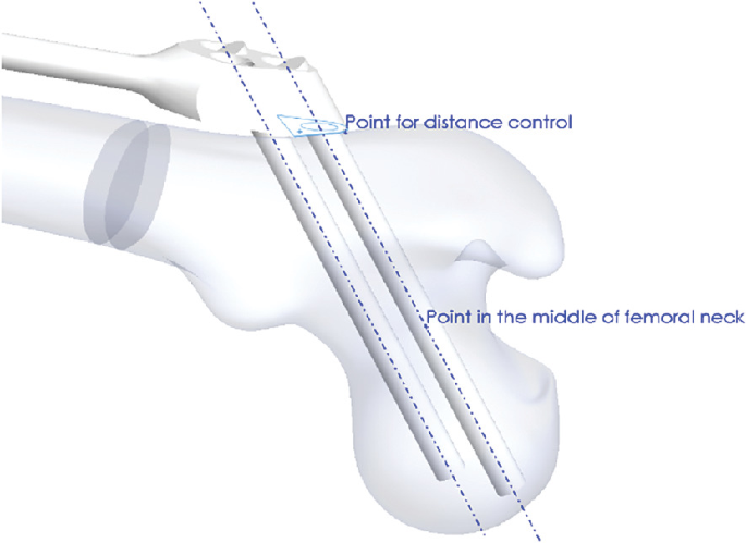

  

  Position of the trochanteric unit on the femur

• 4. The position of the end of the bar, closely following the anatomical axis. It is defined as the coincidence of a point created at an offset from the bar end and a point created in a new empty part in the assembly. The latter point is at the same time coincident with the projection of the anatomical curve onto the femoral surface. Bar end offset point is used instead of the bar end point, to prevent penetration of the bar into the bone and to control the distance of the bar end from the femoral surface.

5 Material Modeling Issues Related to Femur

The accuracy of FEA results largely depends on the accuracy of material models used in the analysis. While it is common to describe standard engineering materials (like steel or aluminum) using homogenous, isotropic, linear elastic material models, describing bone material is a more challenging task. The reason for this lies in the remodeling process that is constantly taking place within the bone tissue. It causes the structure and density of bone tissue to vary through the bone, depending on direction and intensity of stress caused by external loads. Hence, the bone material tends to get pronouncedly inhomogeneous and anisotropic.

Characterization of bone material for FEA is usually done either by zoning the FE model and assigning the averaged material properties to each zone, or by performing so called material mapping, where radiological density values, obtained from CT scans, are used to estimate the values of material constants. Both approaches have their advantages and drawbacks, depending on the application.

Among the factors that affect the accuracy of material characterization, the most important ones are the selection of material model, material properties averaging technique, parameters of x-ray tube, calibration of CT scanner, relations between radiological density and bone density, and relations between bone density and material constants. These are discussed in more detail in (Korunovic et al. 2013).

Usually, bone material is modeled either as linear isotropic or as anisotropic (commonly orthotropic). In a number of studies, it was found that the second approach was more accurate (Baca et al. 2008; Yang et al. 2010). However, it is also true that the characterization and application of anisotropic materials models can represent quite challenging tasks, which may not be worth the extra effort (Peng et al. 2006).

A more detailed description of the two approaches to bone material modeling, that are most often used in FEA, is given in the rest of the section. Those are:

• 1. Zoning, i.e., the division of CAD model into zones that are assigned averaged material characteristics,

• 2. Local material mapping, i.e., assignment of material properties to each finite element separately, where empirical relations between radiological density and bone density, as well as between bone density and elastic constants are used.

According to the first approach, the zones that correspond to the internal femoral structure are created. The zones that can be distinctly separated are compact (cortical) bone, cancellous (trabecular, cancellous) bone and medullary cavity. The zone corresponding to cancellous bone may further be subdivided into zones that are characterized by significantly different trabecular density (Fig. 17.11). While the concept is simple, it has several shortcomings. The main one lies in the fact that the averaged mechanical properties are assigned to the zones spanning quite large areas of the bone, while elastic properties of the bone show significant variation over the bone. For long bones, like tibia or femur, this is especially true. Also, significant effort and time may be required for recognition and creation of zones.

Fig. 17.11

Zones created in the solid CAD model of the femur. For clarity, the zone representing the cortical bone is hidden. Distal segment of cancellous bone is shown in light red. Proximal segment of cancellous bone with sparser trabeculae is shown in light blue. Proximal segments of cancellous bone with denser trabeculae are shown in dark blue and dark red. Medullary cavity is shown in yellow (Korunovic et al. 2010)

According to the second approach, local material mapping, the unique elastic properties are assigned to each finite element, based on local bone tissue density being estimated from CT images. To establish the relations between radiological density (gray values) and bone tissue density, as well as between bone tissue density and elastic constants, empirical equations are used (Schileo et al. 2008; Helgason et al. 2008).

Available FEA programs usually accept a limited number of material property definitions. Thus, the entire range of possible values of an elastic constant (e.g., of Young's modulus), is usually divided into several intervals. Then, a mid-value of the interval to which the calculated value of an elastic constant at the location of a finite element belongs, is assigned to that finite element. In practice, this approach is often used, as it considers local variation of bone density and enables relatively fast creation of FE model. Nevertheless, errors in local characterization of material properties may still be present, especially if the FE mesh is coarse, when the dimensions of some finite elements may get significantly larger than the thickness of particular bone segments.

Both approaches described above had been used throughout authors’ practice in FEA of human femur, as portrayed next.

5.1 Zoning Approach to Material Modeling of the Femur

To represent the cortical bone and medullary cavity, two separate zones in CAD models of the femur were created (Korunovic et al. 2013). The rest of the model, corresponding to spongious bone, was divided into several zones, following the typical trabecular density distribution (Fig. 17.12). The constant values of Young's modulus were assigned to each of the zones, i.e., to the finite elements that were crated inside the zones. To simulate the properties of bone marrow, medullary cavity zone was assigned a very small value of Young's modulus. The values of E_cortical and E_trabecular were determined based on the trial-and-error approach, so that the maximum displacement of the FE model was the same as the displacement of the FE model in which local material mapping was used (as described in Sect. 17.5.2). The resulting FE model, in which the typical element edge size was set to 3 mm and fast element growth from the surface to the interior of the model was used, is shown in Fig. 17.12. Using the mentioned settings, 149,712 tetrahedron elements with quadratic shape functions were created.

Fig. 17.12

The zones and the corresponding FE mesh of the femur model. Green: trabecular bone, E = 12.7 GPa. Red: cancellous bone (denser trabeculae), E = 0.3GPa. White: cancellous bone (sparser trabeculae), E = 0.07 GPa. Yellow: Bone marrow, 1 MPa (Korunovic et al. 2010)

5.2 Local Material Mapping Approach to Material Modeling of the Femur

Based on CT images, only the external surface of the femur was modeled. The volume of the femur was meshed using tetrahedron elements with quadratic shape functions (Fig. 17.13). Once again, the typical element edge size was set to 3 mm and fast element growth from the surface to the interior of the model was used (Korunovic et al. 2013). To assign material properties, local material mapping was performed, based on the following empirical equations: the relation between values of Hounsfield units (HU) and bone density (Eq. 17.1) and the relation between bone density and Young's modulus (Eq. 17.2). Both equations are described in (Morgan et al. 2003). Three different variations of FE model were created, in which 20, 100 or 300 discrete values of Young's modulus were used, as presented in (Korunovic et al. 2013). Using the mentioned settings, 59,926 tetrahedron elements with quadratic shape functions were created.

$$\rho_{app} [g/cm^3 ] = 0.1957 + 0.001053 \, HU$$

(17.1)

$$E[N/mm^2 ] = 6950 \cdot \rho_{app}^{1.49}$$

(17.2)

Fig. 17.13

FE model in which different values of elastic modulus, corresponding to different colors, were assigned to individual finite elements using the local material mapping approach. Lowest values are shown in light blue, while the highest ones are shown in red (Korunovic et al. 2013)

6 Creation of FE Model of Femur-Fixator Assembly

This section describes the FE models of femur-implant assemblies that were used by the authors during the ongoing research. In various studies, different models were built. The choice of the model depended on several factors, like the availability of CT scans, necessary detail level or FE software used. Those models were mutually different by:

• 1. Material modeling of the femur, as described in the previous section. The following models were created:

  • a. Mapped model, which represents a FE model of the femur based on the solid CAD model with outer surface only, where local material mapping is used for the whole model (Fig. 17.13).

  • b. Zoned model with averaged material properties (Fig. 17.12).

  • c. Zoned + mapped model: the model is divided into two zones, one corresponding to cortical bone and the other to the union of the spongious bone and medullary cavity. Mesh is created within each of the zones and material properties assigned by local material mapping. This approach, described in more detail in (Korunovic et al. 2013), is considered to be more accurate than local material mapping alone, as there are no elements that partially belong to the cortical bone volume and partially belong to spongious or medullary cavity volume, and therefore the material property averaging errors are lesser.

  • d. Non-zoned model with averaged material properties, which implies the whole femur volume is assigned a uniform elasticity modulus. This approach is, as a preliminary one, used in creation of flexible and robust femur-SIF assemblies for structural optimization, to simplify the FE model of the femur and concentrate on the CAD model parametrization.

• 2. Landmark creation and model parametrization. The following models were used:

  • a. Non-parametric model, in which the fixator was approximately positioned on femur, according to surgeon’s recommendations.

  • b. Parametric model (Sect. 17.4.2), in which landmarks were created on the femur, and SIF position on the femur was parametrized.

In this section, the procedure for creation of parametric femur-SIF FE model in ABAQUS, with local material mapping, is described, as the one requiring the most steps and user effort. In the first step, the CAD model of the fixator (Fig. 17.14) was created using standard form features such as extruded or revolved cuts and protrusions, holes, chamfers, and rounds. Linear positions and angles of clamps and the length of trochanteric bar were parametrized, to enable the creation of all possible SIF configurations and positions on the femur. This was done because the standard SIF configurations differ by bar length, which may take values of 100 mm, 150 mm, 200 mm, or 250 mm. Also, the clamps are linearly positioned and rotated during the surgery, to adapt to the shape of the femur and fracture position. The CAD model of SIF was assembled with non-parametric CAD model of the femur (created as described in Sect. 17.4.1.). By subtraction of SIF CAD model from femur CAD model, the screw holes in the femur were created (Fig. 17.15).

Fig. 17.14

CAD model of SIF, where bar length equals 150 mm

Fig. 17.15

FE model of femur with material properties assigned (shown in different colors). Screw holes are also visible on the model. Lowest values are shown in light blue, while the highest ones are shown in red (Korunovic et al. 2015)

Next step was the creation of two surface partitions on femoral surface (Fig. 17.17). The surface partition that was created on the head of the femur was later used to define the force acting on the femur as the consequence of the contact with acetabulum. The surface partition that was created on femoral condyles was later used to place the support fixing the lower part of the bone. After the CAD model of the assembly was imported into ABAQUS, two mutually parallel planes were created just below the greater trochanter, to define the limits of the fracture zone. The planes were then used to cut the femur and create the volume that represented a simple subtrochanteric fracture (Fig. 17.17).

Elasticity modulus equal to 1160 N was assigned to the fracture zone, simulating its elasticity 3 weeks after surgery. To simulate the elasticity of the fracture zone 6 and 12 weeks after surgery, values of 2055 N and 4220 N were used respectively. Those values were based on rat femur data reported in (Komatsubara et al. 2005), multiplied by typical ratio of human to rat femoral modules, as no similar studies performed on humans were available. The material of SIF, stainless steel ASTM F 138-2, was characterized by elasticity modulus equal to 2.1 GPa and yield strength of 795 N/mm² (Oldani and Dominguez 2012). The yield strength of cortical bone was set to 112 N/mm², as it was expected to take values between 104 and 120 N/mm² (Ko 1953; Burstein et al. 1976; Vincentelli and Grigoroy 1985). The coefficient of friction between the bone and each component of SIF was set to 0.34 (Mischler and Pax 2002) and between any two components of SIF to 0.7. Temporary material properties, i.e., arbitrary values of Young’s modulus and Poisson’s ratio were assigned to the femur, to enable the creation of the initial FE model. This model was exported from ABAQUS and imported into a medical imaging program in which the material mapping process was performed. One hundred incremental values of Young’s modulus were thereby used, where the lowest one was equal to 1 N/mm² and the highest was equal to 17,500 N/mm² (Fig. 17.15).

After the material mapping procedure was finished, the resulting FE model, containing material properties definitions, was exported from medical imaging software. It was then imported into ABAQUS as “orphan mesh” (containing only finite elements and no geometry), in which it was used to replace the initial FE model within the duplicated femur-SIF assembly model. After the femur model was replaced, contact definitions were lost and thus had to be recreated. Figure 17.16 represents the final FE model of femur-SIF assembly, where each different color corresponds to a fixed value of elasticity modulus. For this reason, the components of SIF and the fracture zone contain the finite elements shown by uniform colors, while the elements belonging to the rest of the femur are shown in many different colors. The number of colors is, in fact, equal to one hundred, as one hundred values of Young’s modulus were used during material mapping.

Fig. 17.16

Final FE model of femur-SIF assembly, containing the fracture zone (Korunovic et al. 2015)

Fig. 17.17

Loads and supports imposed on FE model of femur-SIF assembly. Surface partitions used for load definition, as well as fracture zone are visible in the image (Korunovic et al. 2015)

Loads and supports were defined to resemble the one-legged stance, or more precisely, to mimic the mechanical test that is often performed on cadaveric femurs. On the surface partition that was created in the distal part of the femur, displacement of element nodes was fixed in all directions. On the other surface partition, which was created on the femoral head, a distributed load of 883 N acting in the direction of the mechanical axis was set to simulate the force resulting from body weight of 90 kg (Fig. 17.17).

7 Sensitivity Studies

Previous sections were mostly dedicated to various steps in creation of FE models of femur-implant assembly. After a FE model is built, it is used in structural analysis, to find the values of displacements, strains, stresses or contact pressures of the fixator and of the bone. Those values may be used to predict possible implant failures or bone degradation during the healing process, as it is shown in the following example.

Distribution of equivalent stress, obtained by FEA of a femur-SIF model for a predefined bar size and position of SIF on the femur, where SIF is loaded as depicted in Fig. 17.17, is shown in Fig. 17.18. It may be concluded that the bar and the sliding screws are predominantly loaded in bending.

Fig. 17.18

Equivalent stress in: a femur-SIF assembly, b SIF subassembly (Korunovic et al. 2015)

The highest values of stress, reaching 112.7 N/mm², were found at the upper part of sliding screws and at one of the sliding screws holes in the trochanteric unit. Femur stresses were the highest in the vicinity of screw holes, taking values up to 29.58 N/mm². For the presented SIF configuration and placement, and for the presented load case (one-legged stance), the lowest values of safety factor related to stress were 3.51 on femur and 6.58 on SIF. This leads to the conclusion that the fixator can withstand the imposed loads during the whole healing process.

Previous results are, however, valid only for a specific load case and geometrical configuration of the femur-SIF assembly. During the fracture healing process, fixator is usually exposed to various loading conditions, including dynamic loads. It is, thus, important to identify the situations with highest stresses and to perform accurate modeling of the loads. It may also be important to combine more loading scenarios in one analysis, especially if durability analysis is performed.

Even if all elements of a FE model, including geometry, materials, and loads, are accurately defined, one must bear in mind that the obtained results are valid only for a single specific case. Thus, a single finite element analysis may not be used to find the optimal configuration or placement of the implant, but just to check the validity of the configuration and placement that were determined empirically by the surgeon. To help in surgery planning and decreasing the probability of fixation failure, FEA must be combined with optimization techniques (as described in the next section) or at least a sensitivity study must be performed. A sensitivity study implies changing the values of chosen design variables to observe their influence on mechanical behavior of the structure. If a sensitivity study is to be performed using the FE model of femur-fixator assembly, it is very important that the underlying CAD model, in which the values of design variables are changed to produce the new geometry and update the FE model, is flexible and robust, as described in Sect. 17.4.2.

In the continuation of this section a sensitivity study is presented, which was performed using the FE model based on the CAD model from Sect. 17.4.2. The goal of the study was to find the dependence of SIF stress on the change of two design variables: trochanteric bar length (a) and clamp spacing (b) (Fig. 17.9).

The initial FE model of femur-SIF assembly was based on the CAD model that was configured using the default values of design variables (a = 150 mm and b = 10 mm). The CAD model was imported from Solidworks to ANSYS Workbench (ver. 17.1, Ansys Inc., Canonsburg, PA, USA) via the Workbench associative interface, to establish the bidirectional connection between CAD and FEA models and enable the automatic propagation of geometry changes from CAD to FEA software and vice versa (SolidWorks et al. 2015; Ansys 2016). The details on the FE model and analysis settings may be found in (Korunovic et al. 2019). Loading conditions were set to model the one-legged stance, as described in the previous section.

Sensitivity analysis was performed by defining a design table in ANSYS that contained 16 instances of femur-SIF assembly and running the 16 corresponding analyses continuously. To illustrate the difference between the resulting FE models, the models that correspond to the instances based on minimal and maximal values of design variables are shown in Fig. 17.19.

Fig. 17.19

Sample instances of the FE model of femur–SIF assembly: a Bar length 100 mm, clamp spacing 1 mm. b Bar length 250 mm, clamp spacing 28 mm (Korunovic et al. 2019)²

The values of design variables for each design point (a row in design table corresponding to a different assembly instance), as well as the corresponding value of maximal implant stress, are shown in Table 17.1. The sensitivity of equivalent SIF stress to the change of the two design variables may better be observed in Fig. 17.20, where it is presented in the form of a three-dimensional graph.

Table 17.1 Femur-SIF assembly instances, the values of the design variables, and the calculated values of maximal fixator stress (Korunovic et al. 2019)²

Fig. 17.20

Equivalent stress of SIF, as a function of bar length (a) and clamp spacing (b) (Korunovic et al. 2019)²

Based on Fig. 17.20 it may be concluded that bar length has a significantly larger influence on SIF stress than clamp spacing. For an arbitrary constant value of clamp spacing, SIF stress gets notably larger with shortening of the bar. For an arbitrary constant value of bar length, as clamp spacing gets larger SIF stress gets slightly lower. As only two design variables were defined, and the surface representing the SIF stress as a function of those was smooth and monotonic, even without structural optimization it could be concluded that the optimal values of design variables concerning minimization of SIF stress were a = 250 mm and b = 28 mm. In other words, the surgeon should strive to maximize both bar length and clamp spacing to ensure the maximum durability of SIF if there are no other factors influencing this choice, such as the location of the fracture, the condition of underlying bone or surgical cut length.

8 Optimization Studies

The goal of a structural optimization study is to find the structure that supports the load in the “best” way. For example, the best structure may be sought for transferring a load from a known area in space to a fixed support. For the mathematical optimization to be possible, the term “the best” must be mathematically described in the context of the structure, typically as “minimal mass” or “maximal stiffness”. In each optimization study, one or more functions mathematically define a selected output variable (e.g., displacement, stress, or mass) as a function of design variables. Those are called the objective functions (goals) and are maximized or minimized to find the optimal solution, which is a set of optimal values of design variables. Some constraints must also exist for the optimization task to be fulfilled successfully. For example, if stiffness is maximized without constraints, mass may tend to infinity (Christensen and Klarbring 2008).

There are several types of structural optimization: size, shape, topology, and material optimization. In the case of shape optimization, which is the topic of this section, some of the variable dimensions of the parametric CAD model are considered as design variables. Design variables control the shape of the structure, and their values are changed to achieve targeted mechanical properties i.e., to design the implant having satisfactory structural strength (Milovanovic et al. 2020). It is also possible to include the values of material constants and loads in the shape optimization process. Structural optimization method by which the small segments of material may disappear and reappear is called topology optimization. Resulting geometry is thereby very irregular and organic, as only the necessary parts of the material are kept. It may be very useful in custom implant design, especially if fixators are being produced by additive manufacturing methods that allow great part complexity and design freedom (Cucinotta et al. 2019).{Cucinotta, 2019}.

To find the optimal shape of SIF, response surface optimization (RSO) was performed in DesignXplorer, a module of ANSYS. In RSO, design of experiments (DOE), response surfaces (meta-models), and mathematical optimization methods are used to find the optimal values of design variables (Ansys 2016). The experiments which are required in DOE phase are performed as virtual ones, by means of FEA. Thereby, the underlying CAD model, on which the FE model is based, must be adequately parameterized and robust. Such a model allows the successful creation of any permissible assembly configuration and enables the uninterrupted performance of all required virtual experiments (FEAs).

8.1 Optimization Study 1

In the first study, the exact same model of femur-SIF assembly that was utilized in the sensitivity study described in previous section was used. The goal of this multi-criteria optimization study was to simultaneously minimize the values of maximal equivalent stress of SIF and maximal equivalent stress of femur. The same design variables were kept as in the sensitivity analysis, only in this case the trochanteric bar length was defined as a continuous design variable. The lower and an upper bound of design variables were set as:

• a. Trochanteric bar length (100–250 mm)

• b. Clamp spacing (1–28 mm).

Central composite design (CCD), face centered, enhanced type of DOE was used, resulting in definition of 17 different combinations of design variables values that covered the design space, including extreme points, very well. After all the analyses, i.e., virtual experiments, were finished successfully, response surface of “genetic aggregation” type were fitted to the resulting data. In Fig. 17.21 one of the surfaces is shown together with the data obtained in DOE phase. Similar conclusions may be drawn from this graph as from the one obtained by sensitivity study (Fig. 17.20), suggesting that the inclusion of the femur stress in the optimization did not have significant effect on the results regarding sensitivity.

Fig. 17.21

Equivalent stress of SIF (P10), as a function of bar length (P2) and clamp spacing (P1) obtained by RSO

Finally, the optimization was performed based on the obtained response surface, using the multi-objective genetic algorithm (MOGA). Three sets of optimal values of design variables (candidate points) were obtained, as shown in Table 17.2. The differences between calculated values were minimal, and all the values were close to the ones obtained by sensitivity analysis, i.e., the upper bonds of both design variables. Nevertheless, the first set of design variables values was selected as optimal, since its values of stress were the lowest. In practice, the upper bounds of design variables could be used as optimal values, as they are very close to the results of the optimization.

Table 17.2 Three sets of suggested optimal values obtained by RSO

The previous optimization study did not bring much more benefits than the preceding sensitivity study, except for the automated process of optimal values determination. It is because the optimization task was simple, as only two design variables that were considered had influenced the output variables in a monotonic way.

8.2 Optimization Study 2

The second example presents a more complex optimization study, in which the modified design of SIF and more design variables were considered. Namely, a radius was introduced between the trochanteric unit and the bar, and four extra design variables were created. This was done by allowing the mentioned radius and three more dimensions that were fixed in the standard design to be changed (bar diameter, bar end thickness and bar radius). The suggested modifications of SIF design were made to reduce the stress while lowering the mass of SIF, in order to enhance fixator durability, save material and lower the trauma for the patient. Therefore, the six design variables and their limits were introduced as (Fig. 17.22):

Fig. 17.22

Design variables used in the second optimization study

• P1—Bar length (100–250 mm)

• P2—Bar diameter (8–10 mm)

• P3—Bar end thickness (4–6.5 mm)

• P4—Radius at trochanteric unit (3–10 mm)

• P5—Radius at bar end (6–10 mm)

• P6—Clamp spacing (1–28 mm).

It is a common occurrence that some design variables have a more significant influence on the observed output variables than the other design variables. In addition, performing the optimization study with too many design variables may lead to very long computational times, as there are many virtual experiments to perform. Also, the optimization algorithms may be less efficient when too many variables are used and the optimization results obtained using too many input variables may be tedious to analyze. Therefore, a parameters correlation analysis is often performed to filter out a limited number of the most influential design variables that will be used in design optimization study as input variables. Such an analysis was performed in DesignXplorer and the following variables were selected as the most important ones (the value of calculated Relevance parameter is given in brackets):

• P1—Bar length (1)

• P3—Bar end thickness (1)

• P2—Bar diameter (0.62366).

The other design variables were filtered out, as the values of their Relevance parameters were lower than 0.29, whereas the default threshold was equal to 0.5. The optimization study was therefore performed using the three above design variables and their earlier defined ranges, while the values of other three design variables were fixed at the following values: P4 = 10 mm, P5 = 8 mm, P6 = 28 mm.

Once again, central composite design (CCD), face centered, enhanced type of DOE was used, resulting in definition of 29 different combinations for design variables values. The response surfaces of “genetic aggregation” type were fitted to the resulting data. Some of those are shown in Fig. 17.23, together with the data obtained in DOE phase.

Fig. 17.23

Some of the surfaces obtained in the second optimization study: a equivalent stress of SIF (P8), as a function of bar length (P1) and bar end thickness (P2); b SIF mass (P12), as a function of the same design variables. Both surfaces are shown for the fixed value of bar diameter (P3), equal to 5.25 mm

Detailed results of the RSO are too extensive to be shown. Nevertheless, some conclusions may be drawn from the presented data. Firstly, the response surfaces do not follow the DOE obtained data as closely as in the previous example, which should be expected as the number of design variables is larger. Some data points are very far from the response surface, as, for example, the SIF stress at P1 = 100, P2 = 8 and P3 = 5.25, implying the meta-model has local inaccuracies. There are techniques that may be performed to lessen the surface approximation error, such as creation of verification and refinement points or selection of different response surface type. In this example, the accuracy was considered as acceptable for the optimization to be carried out.

The optimization was performed based on the obtained response surfaces, using the MOGA. Two different sets of objectives and constraints were set. In the first case, the objective was to minimize maximal SIF stress and the constraints were the upper and the lower bounds of design variables. In the second case, two different objectives were defined that had to be satisfied simultaneously: minimization of maximal SIF stress and minimization of SIF mass. The constraints were also the bounds of design variables, plus the upper limit of 220 N/mm² was set as a constraint on SIF stress. The results of the two optimizations are given in Table 17.3, where the shown values of fixator stress are verified by FEA, and in Table 17.4.

Table 17.3 The results of the first optimization task in optimization study 2

Table 17.4 The results of the second optimization task in optimization study 2

In the first case, candidate point 2 has the lowest maximal SIF stress value of 170.32 N/mm², which is considerably lower than the value obtained in the previous study, 208.6 N/mm², when only two design variables were allowed to be changed. The mass is also lower, as it is equal to 0.294 kg and was equal to 0.312 kg. Therefore, it may be concluded that SIF design has been improved both concerning durability and mass. In the second case, the best solution is considered to be candidate point 2, where maximum SIF stress is equal to 216.41 N/mm² and SIF mass equals to 0.253 kg. Here, SIF mass is considerably lower than in the first case and in the previous study, while the maximum SIF stress is a bit higher than in the first optimization study (208.60 N\mm²). As the change of maximum SIF stress is small and the mass is considerably lower, it may be concluded that mass optimization was successful. There is also a possibility to rerun the optimization with changed objectives importance, to emphasize either the mass minimization or the stress minimization objective. In this way, the trade-off between mutually opposite objectives may be controlled.

9 Concluding Remarks

The intention of this chapter was to illustrate how structural analysis based on FEM and structural optimization may jointly be used to plan proximal femoral fracture surgery and to decrease the probability of femoral fixation failures. Various stages in FE model building, structural analysis and structural optimization were illustrated through the studies performed by the authors.

Although the presented methods are well known, the complex freeform geometry of femur, as well as the nature of the bone material, make the creation of FEA models that may be used in automated optimization studies a very complex task. The main challenges lie in creation of flexible and robust CAD models that serve as the basis for FE model creation and in the accurate bone geometry and bone material modeling.

The presented methodology may be used in optimization of various fixation devices utilized in long bone fractures surgical treatment. There is a lot of space for presented methods improvement and many researchers are already working on various related topics. Their ultimate goal is achieving a completely automatic and fast procedure for subject-specific optimization of fixation devices, that would be introduced into clinical practice.

References

Almeida D, Ruben R, Folgado J, Fernandes P, Audenaert E, Verhegghe B, De Beule M (2016) Fully automatic segmentation of femurs with medullary canal definition in high and in low resolution CT scans. Med Eng Phys 38(12):1474–1480
Almeida D, Ruben R, Folgado J, Fernandes P, Gamelas J, Verhegghe B, De Beule M (2017) Automated femoral landmark extraction for optimal prosthesis placement in total hip arthroplasty. International Journal for Numerical Methods in Biomedical Engineering, 33(8):e2844
Ansys C (2016) Reference Guide, Release 17.1. ANSYS Inc., Canonsburg, PA
Baca V, Horak Z, Mikulenka P, Dzupa V (2008) Comparison of an inhomogeneous orthotropic and isotropic material models used for FE analyses. Med Eng Phys 30(7):924–930
Burstein AH, Reilly DT, Martens M (1976) Aging of bone tissue: mechanical properties. The J Bone Joint Surg Am 58(1):82–86
Chang K-H (2014) Product design modeling using CAD/CAE: the computer aided engineering design series. Academic Press
Christensen P, Klarbring A (2008) An introduction to structural optimization, vol 153. Springer Science & Business Media
Cucinotta F, Guglielmino E, Longo G, Risitano G, Santonocito D, Sfravara F (2019) Topology optimization additive manufacturing-oriented for a biomedical application. In: Advances on mechanics, design engineering and manufacturing II. Springer. pp 184–193
Eberle S, Gerber C, Von Oldenburg G, Högel F, Augat P (2010) A biomechanical evaluation of orthopaedic implants for hip fractures by finite element analysis and in-vitro tests. Proc Inst Mech Eng [h] 224(10):1141–1152
Edwards B, Miller R, Derrick T (2016) Femoral strain during walking predicted with muscle forces from static and dynamic optimization. J Biomech 49(7):1206–1213
Ehlke M, Ramm H, Lamecker H, Hege H-C, Zachow S (2013) Fast generation of virtual X-ray images for reconstruction of 3D anatomy. IEEE Trans Visual Comput Graphics 19(12):2673–2682
Floyd J, O'toole R, Stall A, Forward D, Nabili M, Shillingburg D, Hsieh A, Nascone J (2009) Biomechanical comparison of proximal locking plates and blade plates for the treatment of comminuted subtrochanteric femoral fractures. J Orthop Trauma 23(9):628–633
Helgason B, Perilli E, Schileo E, Taddei F, Brynjólfsson S, Viceconti M (2008) Mathematical relationships between bone density and mechanical properties: a literature review. Clin Biomech 23(2):135–146
Hibbeler RC, Kiang T (2015) Structural analysis. Pearson Prentice Hall Upper Saddle River
Kainmueller D, Lamecker H, Zachow S, Hege H-C An articulated statistical shape model for accurate hip joint segmentation. In: Engineering in medicine and biology society, 2009. EMBC 2009. Annual international conference of the IEEE, 2009. IEEE. pp 6345–6351
Ko R (1953) The tension test upon the compact substance of the long bones of human extremities. J Kyoto Pref Med Univ 53:503
Komatsubara S, Mori S, Mashiba T, Nonaka K, Seki A, Akiyama T, Miyamoto K, Cao Y, Manabe T, Norimatsu H (2005) Human parathyroid hormone (1–34) accelerates the fracture healing process of woven to lamellar bone replacement and new cortical shell formation in rat femora. Bone 36(4):678–687
Konya M, Verim Ö (2017) Numerical optimization of the position in femoral head of proximal locking screws of proximal femoral nail system; biomechanical study. Balkan Med J 34(5):425
Korunovic N, Marinkovic D, Trajanovic M, Zehn M, Mitkovic M, Affatato S (2019) In silico optimization of femoral fixator position and configuration by parametric CAD model. Materials 12(14):2326
Korunovic N, Trajanovic M, Mitkovic M, Vulovic S (2010) From CT scan to FEA model of human femur. IMK-14-Istrazivanje i razvoj 16(2):45–48 (in Serbian)
Korunovic N, Trajanovic M, Stevanovic D, Vitkovic N, Stojkovic M, Milovanovic J, Ilic D Material characterization issues in FEA of long bones. In: SEECCM III 3rd South-East European conference on computational mechanics—an ECCOMAS and IACM special interest conference, Kos Island, Greece, 2013, pp 12–14
Korunovic N, Trajanovic M, Mitkovic M, Vitkovic N, Stevanovic D (2015) A parametric study of selfdynamisable internal fixator used in femoral fracture treatment. Paper presented at the NAFEMS world congress 2015 inc. 2nd International SPDM Conference, San Diego, 21–24 June
Lunsjö K, Ceder L, Tidermark J, Hamberg P, Larsson B-E, Ragnarsson B, Knebel RW, Allvin I, Hjalmars K, Norberg S (1999) Extramedullar fixation of 107 subtrochanteric fractures: a randomized multicenter trial of the Medoff sliding plate versus 3 other screw-plate systems. Acta Orthop Scand 70(5):459–466
Micic I, Mitkovic M, Park I-H, Mladenovic D, Stojiljkovic P, Golubovic Z, Jeon I-H (2010) Treatment of subtrochanteric femoral fractures using selfdynamisable internal fixator. Clin Orthop Surg 2(4):227–231
Milovanovic J, Stojkovic M, Husain K, Korunovic N, Arandjelovic J (2020) Holistic approach in designing the personalized bone scaffold: the case of reconstruction of large missing piece of mandible caused by congenital anatomic anomaly. J Healthc Eng 2020:6689961
Mischler S, Pax G (2002) Tribological behavior of titanium sliding against bone. Eur Cell Mater 3(1):28–29
Mitkovic M, Milenkovic S, Micic I, Mladenovic D, Mitkovic M (2012) Results of the femur fractures treated with the new selfdynamisable internal fixator (SIF). Eur J Trauma Emerg Surg 38(2):191–200
Mittal R, Banerjee S (2012) Proximal femoral fractures: principles of management and review of literature. J Clin Orthop Trauma 3(1):15–23
Morgan EF, Bayraktar HH, Keaveny TM (2003) Trabecular bone modulus—density relationships depend on anatomic site. J Biomech 36(7):897–904
Oldani C, Dominguez A (2012) Titanium as a biomaterial for implants. Recent Adv Arthroplasty 218:149–162
Pakhaliuk V, Poliakov A (2018) Simulation of wear in a spherical joint with a polymeric component of the total hip replacement considering activities of daily living. Facta Universitatis-Ser Mech Eng 16(1):51–63
Pavic A, Kodvanj J, Surjak M (2013) Determining the stability of novel external fixator by using measuring system Aramis. Tehnički Vjesnik 20(6):995–999
Peng L, Bai J, Zeng X, Zhou Y (2006) Comparison of isotropic and orthotropic material property assignments on femoral finite element models under two loading conditions. Med Eng Phys 28(3):227–233
Perren S (2002) Evolution of the internal fixation of long bone fractures: the scientific basis of biological internal fixation: choosing a new balance between stability and biology. J Bone Joint Surg Br 84(8):1093–1110
Petrovic S, Korunovic N (2018) Imaging in clinical and preclinical practice. In: Biomaterials in clinical practice. Springer, pp 539–572
Phillips A (2009) The femur as a musculo-skeletal construct: a free boundary condition modelling approach. Med Eng Phys 31(6):673–680
Samsami S, Saberi S, Sadighi S, Rouhi G (2015) Comparison of three fixation methods for femoral neck fracture in young adults: experimental and numerical investigations. J Med Biol Eng 35(5):566–579
Schileo E, Dall’Ara E, Taddei F, Malandrino A, Schotkamp T, Baleani M, Viceconti M (2008) An accurate estimation of bone density improves the accuracy of subject-specific finite element models. J biomech 41(11):2483–2491
SolidWorks DS, Street W, Waltham M (2015) SOLIDWORKS 2016. Online help. Accessed Mar 2020
Sowmianarayanan S, Chandrasekaran A, Kumar K (2008) Finite element analysis of a subtrochanteric fractured femur with dynamic hip screw, dynamic condylar screw, and proximal femur nail implants - a comparative study. Proc Inst Mech Eng [h] 222(1):117–127
Stojkovic M, Trajanovic M, Vitkovic N, Milovanovic J, Arsić S, Mitković M (2009) Referential geometrical entities for reverse modeling of geometry of femur. Paper presented at the VIPIMAGE 2009, Porto, Portugal
Vincentelli R, Grigoroy M (1985) The effect of Haversian remodeling on the tensile properties of human cortical bone. J Biomech 18(3):201–207
Vitkovic N, Milovanovic J, Korunovic N, Trajanovic M, Stojkovic M, Mišic D, Arsic S (2013) Software system for creation of human femur customized polygonal models. Comput Sci Inf Syst 10(3):1473–1497
Vulovic S, Korunovic N, Trajanovic M, Grujovic N, Vitkovic N (2011) Finite element analysis of CT based femur model using finite element program PAK. J Serb Soc Comput Mech 5(2):160–166
Wu X, Yang M, Wu L, Niu W (2015) A biomechanical comparison of two intramedullary implants for subtrochanteric fracture in two healing stages: a finite element analysis. Appl Bionics Biomech 2015
Yang H, Ma X, Guo T (2010) Some factors that affect the comparison between isotropic and orthotropic inhomogeneous finite element material models of femur. Med Eng Phys 32(6):553–560
Zou Z, Liao S-H, Luo S-D, Liu Q, Liu S-J (2017) Semi-automatic segmentation of femur based on harmonic barrier. Comput Methods Programs Biomed 143:171–184
Acknowledgments
This research was financially supported by the Ministry of Education, Science and Technological Development of the Republic of Serbia (Agreement no. 451-03-9/2021-14/200109).
Author information
Authors and Affiliations
Corresponding author
Editor information
Editors and Affiliations
Rights and permissions
Copyright information
© 2022 The Author(s), under exclusive license to Springer Nature Switzerland AG
About this chapter
Cite this chapter
Korunovic, N., Arandjelovic, J. (2022). Structural Analysis and Optimization of Fixation Devices Used in Treatment of Proximal Femoral Fractures. In: Canciglieri Junior, O., Trajanovic, M.D. (eds) Personalized Orthopedics. Springer, Cham. https://doi.org/10.1007/978-3-030-98279-9_17
Download citation
DOI: https://doi.org/10.1007/978-3-030-98279-9_17
Published:
Publisher Name: Springer, Cham
Print ISBN: 978-3-030-98278-2
Online ISBN: 978-3-030-98279-9
eBook Packages: EngineeringEngineering (R0)