A Tale of Three Families: Discriminative, Descriptive, and Generative Models

Abstract

This chapter gives a general introduction to three families of probabilistic models and their connections. Most of the models studied in the previous chapters, as well as most of the models in the current machine learning and deep learning literature, belong to these three families of models.

12.1 Introduction

12.1.1 Three Families of Probabilistic Models

This chapter gives a general introduction to three families of probabilistic models and their connections. Most of the models studied in the previous chapters, as well as most of the models in the current machine learning and deep learning literature, belong to these three families of models.

The first class consists of discriminative models or classifiers that are commonly used in supervised learning. The second class consists of descriptive models—also known as energy-based models—that define unnormalized probability density functions in the data space. These models are generalizations of the FRAME model introduced in the previous chapters. The third class consists of generative models that are directed top-down models that involve latent variables. The generative models are generalizations of factor analysis and its variants. They are also called directed graphical models.

About the names of the models, we use the term “generative models” in a much narrower sense than in the current literature. They refer to top-down models that consist of latent variables that follow simple prior distributions so that the examples can be directly generated. As to the “descriptive models,” they refer to the energy-based models or deep FRAME model introduced in the previous chapter. They only describe the examples in terms of their probability densities, but they cannot directly generate the examples. The generative task is left to iterative MCMC sampling algorithms. Therefore, these models are not literally generative as they do not explicitly define a generative process, and that is why we call them descriptive.

$$\displaystyle \begin{aligned} \begin{array}{rcl} \begin{array}[c]{ccccc} \mathit{{Top-down mapping}} && \mathit{{Bottom-up mapping}} && \mathit{{Bottom-up mapping}} \\ \mbox{latent variables }z && \mbox{log density }f_\theta(x) && \mbox{logit score (density ratio)}\\ \Downarrow&&\Uparrow &&\Uparrow\\ \mbox{example }x \approx g_\theta(z) && \mbox{example }x && \mbox{example }x \\ \mbox{(a) }{\mathbf{Generative}}\mbox{ (sampler) }&& \mbox{(b) }{\mathbf{Descriptive}}\mbox{ (density)} && \mbox{(b) }{\mathbf{Discriminative}}\mbox{ (classifier)} \end{array} {} \end{array} \end{aligned} $$

(12.1)

Density vs. Sampler

A descriptive model specifies the probability density function explicitly, up to a normalizing constant. A discriminative model specifies the ratios between two or more densities via the Bayes rule. A generative model, on the other hand, does not specify a data density explicitly. It specifies a sampler or a sampling process that transforms latent variables with a known distribution, e.g., Gaussian white noise variables, to the observed example. By analogy to reinforcement learning, a density is like a value network or a critic, and a sampler is like a policy network or an actor.

The above diagram illustrates the three families of probabilistic models. A generative model is based on a top-down mapping from the latent variables z to the example x. A descriptive model is based on a bottom-up mapping from the example x to the log of the unnormalized density. A discriminative model is based on a bottom-up mapping from the example x to the logit score that is also the ratio between the densities of positive and negative classes in the binary classification situation (which can be easily generalized to the multi-class situation). All the mappings can be parameterized by deep neural networks.

In the previous chapter, we introduced the descriptive models and generative models for image and video data and the associated maximum likelihood learning algorithms. This chapter will give a more general treatment. We shall still emphasize the maximum likelihood learning algorithm. Meanwhile, we shall also present various joint training schemes, such as variational learning and adversarial learning. We shall make this chapter self-contained so that readers who are interested in the development in the deep learning era can read this chapter in isolation.

Notation

We shall adopt the notation commonly used in the current literature. We use x to denote the training example, e.g., an image or a sentence. We use z to denote the latent variables in the generative model. We use y to denote the output in the discriminative model, e.g., image category. We use θ to denote the model parameters. We use the notations ∇_x and ∇_θ to denote $\frac {\partial }{\partial x}$ and $\frac {\partial }{\partial \theta }$, respectively. For a function h(θ), its derivative at a fixed value, say, θ_t, is denoted ∇_θh(θ_t). We use D_KL to denote the Kullback–Leibler divergence.

12.1.2 Supervised, Unsupervised, and Self-supervised Learning

Supervised learning refers to the situation where both the input x and the output y are given, and we want to learn to predict y based on x. More formally, we learn a discriminative or predictive model p(y|x) by maximum likelihood, i.e., we maximize the average of $\log p(y|x)$ over the model parameters where the average is over the training set {x, y}. The limitation of supervised learning is that it can be expensive and time-consuming to obtain y in the form of label or annotation.

Unsupervised learning refers to the situation where only the input x is given, but the output y is unavailable. In that case, we can learn a descriptive model or a generative model, again by maximum likelihood, but we maximize the average of $\log p(x)$ over the model parameters, where the average is over the training set {x}, instead of the average of $\log p(y|x)$, as y is not available. The descriptive model specifies p(x) up to an unknown normalizing constant, and it is closely related to the discriminative model through the Bayes rule. For the generative model, p(x) is implicit because it involves integrating out the latent variables z. The latent z can be inferred from the input x.

Semi-supervised learning refers to the situation between supervised and unsupervised learning, where there are a small number of labeled examples where both x and y are given, and there are a large number of unlabeled examples where only x is given. In that case, we can again learn the model by maximum likelihood, where we maximize the sum of $\log p(y|x)$ over the labeled examples and $\log p(x)$ over the unlabeled examples. Thus probabilistic modeling provides a unified likelihood-based framework for supervised, unsupervised, and semi-supervised learning.

There is also self-supervised learning, which is to translate unsupervised learning into supervised learning. Specifically, even if we are only given x without y, we can nonetheless create a task where we artificially introduce y for a modification of x that depends on y, and we then learn p(y|x) instead of p(x). This type of learning can be more formally treated as learning descriptive model by various conditional likelihoods.

12.1.3 MCMC for Synthesis and Inference

Although likelihood-based learning with probabilistic models is a principled framework for supervised, unsupervised, and semi-supervised learning, the bottleneck for likelihood-based learning for unsupervised learning is that the derivative of the log-likelihood function $\log p(x)$ usually involves intractable integrals or expectations, which require expensive MCMC sampling. A lot of effort has been spent on getting around this obstacle.

We may use short-run MCMC, i.e., running MCMC such as Langevin dynamics or Hamiltonian Monte Carlo (HMC) [179] from a fixed initial noise distribution for a fixed number of steps, for inference and synthesis computations. This is affordable on modern computing platforms. It can also be justified as a modification or perturbation of the maximum likelihood learning.

Short-run MCMC is convenient for learning models with multiple layers of latent variables organized in complex architectures because top-down feedback and lateral inhibition between the latent variables at different layers can automatically emerge in short-run MCMC. The short-run Langevin dynamics can also be compared with attractor dynamics that is a commonly assumed framework for modeling neural computations [7, 108, 198]. One can also run persistent Markov chains, i.e., in each learning iteration, we initialize finite-step MCMC from the samples generated in the previous learning iteration.

12.1.4 Deep Networks as Function Approximators

All three classes of models can be parameterized by deep neural networks [138, 144], which are compositions of multiple layers of linear transformations and coordinate-wise nonlinear transformations.

Specifically, consider a nonlinear transformation f(x) that can be decomposed recursively as s_l = W_lh_l−1 + b_l, and h_l = r_l(s_l), for l = 1, …, L, with f(x) = h_L and h₀ = x. W_l is the weight matrix at layer l, and b_l is the bias vector at layer l. Both s_l and h_l are vectors of the same dimensionality, and r_l is a one-dimensional nonlinear function, or rectification function, that is applied coordinate-wise or element-wise.

The nonlinear rectification is crucial for f(x) to approximate nonlinear mapping. In the past, the nonlinear rectification r_l() is usually sigmoid transformation, which is approximately a two-piece constant function. This makes f(x) approximately piecewise constant function. Modern deep networks usually use $r_l(s) = \max (0, s)$, the rectified linear unit or ReLU, which makes f(x) piecewise linear.

There are two special classes of neural networks. One consists of convolutional neural networks [138, 144], which are commonly applied to images, where the same linear transformations are applied around each pixel locally. The other class consists of recurrent neural networks [103], which are commonly applied to sequence data such as speech and natural language. Recently, the transformer model [239] has become the most prominent architecture.

Deep neural networks are powerful function approximators that can approximate highly nonlinear high-dimensional continuous functions by interpolating training examples. Modern deep networks are highly overparameterized, meaning that the number of parameters greatly exceeds the number of training examples. Thus they have enough capacity to fit the training data, yet they tend not to overfit the training data because the networks are learned by stochastic gradient descent algorithm where the gradient is computed via back-propagation. The stochastic gradient descent algorithm provides implicit regularization [11, 221].

12.1.5 Learned Computation

Because of the strong approximation capacity, the boundary between representation and computation is rather blurred because a deep network can approximate an iterative algorithm. Sometimes this is called learned computation.

In fact, the residual network [97] can be considered a finite-step iterative algorithm. It is of the form x_l+1 = x_l + f_l(x_l), where l indexes the layer. Meanwhile, l may also be interpreted as time step of an iterative algorithm, i.e., we can also write x_t+1 = x_t + f_t(x_t), which is to model iterative updating or refinement. In general, it can be interpreted as a mixture of both, i.e., there is actually a small number of layers, and each layer is computed by a finite-step iterative algorithm.

The transformer model [239] can also be considered a finite-step iterative algorithm that iteratively updates the vector representations of the words of an input sentence through the self-attention mechanism where the words pay attention to and gather information from each other. The graph convolutional network [134] can learn the iterative message passing mechanism where the nodes of the graph send messages to each other.

In the above iterative updating mechanisms, there is no need to know the objective functions of these iterative mechanisms. They can be embedded into a classifier and be trained by the classification loss via back-propagation through time.

12.1.6 Amortized Computation for Synthesis and Inference Sampling

Even if there is an objective function, we can still learn a deep network that directly maps the input to an approximate solution. Sometimes this is called amortized computation, which seeks to approximate an iterative algorithm of multiple time steps.

In the case of the generative model, recall that we can use short-run MCMC as an approximate sampler for synthesis and inference. We can also learn a network that produces the samples directly. In the case of posterior sampling, this is referred to as variational inference model [133]. In fact, the short-run MCMC can be considered a noise-injected residual network.

When there are multiple layers of latent variables, designing a network for approximate inference sampling can be a non-trivial task, whereas short-run MCMC remains automatic.

12.1.7 Distributed Representation and Embedding

Deep neural networks are based on continuous vectors and weight matrices. They are highly interpolative and amendable to gradient-based computations. On the other hand, high-level reasoning can also be highly symbolic, with symbols, logic, and grammar. For a dictionary of symbols, each symbol can be represented by a one-hot vector, and a small subset of symbols selected from the dictionary can be represented by a sparse vector. This is in contrast to the vectors in deep networks, which are continuous and dense. Such vectors are called distributed representations. They are also commonly referred to as embeddings. For instance, the word2vec model [172, 193] represents each word by a dense vector, and this means we embed the words in a continuous Euclidean space. A modern deep network such as transformer [239] or graph neural network [134] can be viewed as a team of vectors, which are operated on by learned matrices so that they can pass on messages to each other. For discrete or symbolic inputs or outputs such as words or tokens, they can be encoded into vectors or decoded from the vectors.

It is still unclear how to unify symbolic and dense representations. Sometimes this is referred to as the contrast between symbolism and connectionism. It is likely that there is a duality or complementarity between sparse vectors and dense vectors, and each is more convenient and efficient than the other depending on the scenario.

12.1.8 Perturbations of Kullback–Leibler Divergence

A unifying theoretical device for studying various learning methods is to perturb the Kullback–Leibler divergence for maximum likelihood by other Kullback–Leibler divergences. This scheme consists of three Kullback–Leibler divergences: (1) KL-divergence underlying maximum likelihood learning. This is the target of the perturbations. (2) KL-divergence underlying synthesis sampling. (3) KL-divergence underlying inference sampling. (2) and (3) are perturbations that are applied to (1). The sign in front of (2) is negative, and the sign in front of (3) is positive.

The above theoretical framework explains the following learning algorithms: (1) The maximum likelihood learning algorithm. (2) The learning algorithm based on short-run MCMC for synthesis and inference. (3) The learning methods based on learned networks for synthesis and inference, including adversarial learning [81] and variational learning [133].

12.1.9 Kullback–Leibler Divergence in Two Directions

To be more specific, recall that for two probability densities p(x) and q(x), we define

$$\displaystyle \begin{aligned} \begin{array}{rcl} D_{\mathrm{KL}}(p \| q) = {\mathrm{E}}_p\left[ \log \frac{p(x)}{q(x)}\right] = \int p(x) \log \frac{p(x)}{q(x)} dx. \end{array} \end{aligned} $$

(12.2)

The KL-divergence appears in two scenarios:

• (1) Maximum likelihood learning. Suppose the training examples x_i ∼ p_data(x) are independent for i = 1, …, n. Suppose we want to learn a model p_θ(x). The log-likelihood function is

  $$\displaystyle \begin{aligned} \begin{array}{rcl} L(\theta) = {\frac{1}{n} \sum_{i=1}^{n}} \log p_\theta(x_i) \rightarrow {\mathrm{E}}_{{p_{\mathrm{data}}}}[\log p_\theta(x)]. \end{array} \end{aligned} $$

  (12.3)

  Thus for big n, maximizing L(θ) is equivalent to minimizing

  $$\displaystyle \begin{aligned} D_{\mathrm{KL}}({p_{\mathrm{data}}} \|p_\theta) = -{\mathrm{entropy}}({p_{\mathrm{data}}}) - {\mathrm{E}}_{{p_{\mathrm{data}}}}[\log p_\theta(x)] \doteq -{\mathrm{entropy}}({p_{\mathrm{data}}}) - L(\theta), \end{aligned} $$

  (12.4)

  where ${\mathrm {E}}_{{p_{\mathrm {data}}}}$ can be approximated by averaging over {x_i}. We can think of it as projecting p_data onto the model space {p_θ, ∀θ}.

  For the rest of this chapter, for notational simplicity, we will not distinguish between ${\mathrm {E}}_{{p_{\mathrm {data}}}}$ and sample average over {x_i}, and we will treat D_KL(p_data∥p_θ) as the loss function for maximum likelihood learning.

• (2) Variational approximation. Suppose we have a target distribution p_target, and we know p_target up to a normalizing constant, e.g., $p_{\mathrm {target}}(x) = \exp (f(x))/Z$, where we know f(x) but the normalizing constant $Z = \int \exp (f(x)) dx$ is analytically intractable. Suppose we want to approximate it by a distribution q_ϕ. We can find ϕ by minimizing

  $$\displaystyle \begin{aligned} \begin{array}{rcl} {} D_{\mathrm{KL}}(q_\phi \| p_{\mathrm{target}}) = {\mathrm{E}}_{q_\phi}[\log q_\phi(x)] - {\mathrm{E}}_{q_\phi}[ f(x)] + \log Z. \end{array} \end{aligned} $$

  (12.5)

  This time, we place q_ϕ on the left-hand side and p_target on the right-hand side of the KL-divergence, because p_target is accessible only through f(x). The above minimization does not require knowledge of $\log Z$.

The behaviors of min_θD_KL(p_data∥p_θ) in (1) and min_ϕD_KL(q_ϕ∥p_target) in (2) are different. In (1), p_θ tends to cover all the modes of p_data because D_KL(p_data∥p_θ) is the expectation with respect to p_data. In (2), q_ϕ tends to focus on some major modes of p_target, while ignoring the minor modes, because D_KL(q_ϕ∥p_target) is the expectation with respect to q_ϕ.

In the perturbation scheme mentioned in the previous subsection, the KL-divergence for maximum likelihood is (12.4). The perturbations are of the form in (12.5).

12.2 Descriptive Energy-Based Model

12.2.1 Model and Origin

Let x be a training example, e.g., an image or a sentence. A descriptive model specifies an unnormalized probability density function

$$\displaystyle \begin{aligned} \begin{array}{rcl} p_\theta(x) = \frac{1}{Z(\theta)} \exp(f_\theta(x)), \end{array} \end{aligned} $$

(12.6)

where f_θ(x) is parameterized by a deep network, with θ collecting all the weight and bias parameters. $Z(\theta ) = \int \exp (f_\theta (x)) dx$ is the normalizing constant.

Such a model originated from statistical mechanics and is called the Gibbs distribution, where x is the state or configuration of a physical system, and − f_θ(x) is the energy function of the state so that the lower energy states are more likely to be observed. For that reason, the above model is also called energy-based model (EBM) in the literature [32, 70, 99, 161, 180, 182, 184, 266, 269, 270].

In classical mechanics, the configuration x(t) evolves deterministically over time t according to a partial differential equation. Then where does the probability distribution come from? We may consider the ensemble or population (x(t), t ∈ [t₀, t₁]), for a long enough burn-in time t₀ and long enough duration t₁ − t₀. For a random time t ∼Uniform[t₀, t₁], x(t) follows a probability distribution p(x), and it can be modeled by a Gibbs distribution.

The quantity Z(θ) is called the partition function in statistical mechanics. An important identity is

$$\displaystyle \begin{aligned} \begin{array}{rcl} \nabla_\theta \log Z(\theta) = {\mathrm{E}}_{p_\theta}[ \nabla_\theta f_\theta(x)]. \end{array} \end{aligned} $$

(12.7)

The non-differentiability of $\log Z(\theta )$ underlies the phase transition phenomena in statistical physics.

The descriptive model has strong expressive power because it only needs to specify a scalar-valued function f_θ(x). f_θ(x) is like an objective function (or value function, or constraints, or rules). The descriptive model is only responsible for specifying the objective function and is not responsible for optimizing the objective function or providing near-optimal solutions. The latter task is left to MCMC sampling. As a result, a simple descriptive model p_θ(x) or the objective function f_θ(x) can explain rich patterns and complex behaviors.

The descriptive model has been used for inverse reinforcement learning, where − f_θ(x) serves as the cost function [283]. It has also been used for Markov logic network [204], where f_θ(x) combines logical rules.

12.2.2 Gradient-Based Sampling

For high-dimensional x, such as image, sampling from p_θ(x) requires MCMC, such as Langevin dynamics or Hamiltonian Monte Carlo. The Langevin dynamics iterates

$$\displaystyle \begin{aligned} \begin{array}{rcl} x_{t+1} = x_t + s \nabla_x f_\theta(x_t) + \sqrt{2 s} e_t, \end{array} \end{aligned} $$

(12.8)

where s is the step size and e_t ∼N(0, I) is the Gaussian white noise term. The Langevin dynamics has a gradient ascent term ∇_xf_θ(x_t), and e_t is the diffusion term for randomness. As s → 0 and t →∞, the distribution of x_t converges to p_θ(x).

We can write the Langevin dynamics in continuous time as

$$\displaystyle \begin{aligned} \begin{array}{rcl} x_{t + \Delta t} = x_t + \frac{1}{2} \nabla_x f_\theta(x_t) \Delta t + \sqrt{\Delta t} e_t, \end{array} \end{aligned} $$

(12.9)

or more formally,

$$\displaystyle \begin{aligned} \begin{array}{rcl} d x_t = \frac{1}{2} \nabla_x f_\theta(x_t) dt + d B_t, \end{array} \end{aligned} $$

(12.10)

where dB_t plays the role of $\sqrt {\Delta t} e_t$.

Let p_t be the distribution of x_t. Then according to the Fokker–Planck equation, we have

$$\displaystyle \begin{aligned} \begin{array}{rcl} \nabla_t p_t(x) = \frac{1}{2} [ \nabla_x (f_\theta(x) p_t(x)) + \nabla^2_x p_t(x)]. \end{array} \end{aligned} $$

(12.11)

p_θ(x) is the solution to ∇_tp_t(x) = 0, i.e., the stationary distribution. In terms of variational approximation,

$$\displaystyle \begin{aligned} \begin{array}{rcl} D_{\mathrm{KL}}(p_t \| p_\theta) = -{\mathrm{entropy}}(p_t) - {\mathrm{E}}_{p_t}[f_\theta(x)] + \log Z(\theta) \rightarrow 0 \end{array} \end{aligned} $$

(12.12)

monotonically as t →∞ under fairly general conditions. The gradient term in the Langevin dynamics increases f_θ(x) or decreases energy, while the noise term e_t increases the entropy of p_t.

Intuitively, imagine a population of x’s that are distributed according to p_θ(x). The deterministic gradient ascent term in the Langevin dynamics pushes the points toward the local modes of the log density, making the distribution of the points more focused on the local modes of the density. Meanwhile, the random diffusion term in the Langevin dynamics adds random noises to the points, making the distribution of the points more diffused from the local modes of the density. The two terms balance each other so that the overall distribution of the points after each Langevin iteration remains unchanged.

Hamiltonian Monte Carlo (HMC) [105, 179] is a more powerful gradient-based MCMC sampling method. Similar to gradient descent with momentum, it can navigate the high curvature regions of the energy landscape more smoothly and efficiently. The step size in HMC can be adaptively selected based on the acceptance rate calculated from the energy function [105].

In order to traverse local modes and facilitate fast mixing of the Markov chain, one can add a temperature parameter to interpolate the multi-modal target density and a simple unimodal reference density such as Gaussian white noise distribution. One can then use simulated annealing [135] or more principled and effective MCMC schemes such as simulated tempering [168], parallel tempering [48, 77], or replica exchange [226] to sample from multi-modal density.

12.2.3 Maximum Likelihood Estimation (MLE)

The descriptive model p_θ(x) can be learned by maximum likelihood estimation (MLE). The log-likelihood is the average of

$$\displaystyle \begin{aligned} \begin{array}{rcl} \log p_\theta(x) = f_{\theta}(x) - \log Z(\theta), \end{array} \end{aligned} $$

(12.13)

where the average is over the training set {x}. The gradient of $\log p_\theta (x)$ with respect to θ is

$$\displaystyle \begin{aligned} \begin{array}{rcl} \delta_\theta(x) = \nabla_\theta \log p_\theta(x) = \nabla_\theta f_{\theta}(x) - {\mathrm{E}}_{p_\theta(x)} [ \nabla_\theta f_{\theta}(x)], \end{array} \end{aligned} $$

(12.14)

where

$$\displaystyle \begin{aligned} \begin{array}{rcl} \nabla_\theta \log Z(\theta) = {\mathrm{E}}_{p_\theta(x)}[\nabla_\theta f_{\theta}(x)]. \end{array} \end{aligned} $$

(12.15)

Suppose we observe training examples {x_i, i = 1, …, n}∼ p_data, where p_data is the data distribution. For large n, the sample average over {x_i} approximates the expectation with respect to p_data. For notational convenience, we treat the sample average and the expectation as the same.

The log-likelihood is

$$\displaystyle \begin{aligned} \begin{array}{rcl} {} L(\theta) = {\frac{1}{n} \sum_{i=1}^{n}} \log p_\theta(x_i) \doteq {\mathrm{E}}_{{p_{\mathrm{data}}}}[ \log p_\theta(x)]. \end{array} \end{aligned} $$

(12.16)

The derivative of the log-likelihood is

$$\displaystyle \begin{aligned} L^{\prime}(\theta) = {\mathrm{E}}_{{p_{\mathrm{data}}}}[\delta_\theta(x)] &= {\mathrm{E}}_{{p_{\mathrm{data}}}} \left[ \nabla_\theta f_\theta(x)\right] - {\mathrm{E}}_{p_\theta} \left[ \nabla_\theta f_\theta(x) \right] \end{aligned} $$

(12.17)

$$\displaystyle \begin{aligned} &\doteq {\frac{1}{n} \sum_{i=1}^{n}} \nabla_\theta f_\theta(x_i) - {\frac{1}{n} \sum_{i=1}^{n}} \nabla_\theta f_\theta(x_i^{-}), \end{aligned} $$

(12.18)

where $x_i^{-} \sim p_\theta (x)$ for i = 1, …, n are the generated examples from the current model p_θ(x).

The above equation leads to the “analysis by synthesis” learning algorithm. At iteration t, let θ_t be the current model parameters. We generate synthesized examples $x_i^{-} \sim p_{{\theta }_t}(x)$ for i = 1, …, n. Then we update θ_t+1 = θ_t + η_tL^′(θ_t), where η_t is the learning rate, and L^′(θ_t) is the statistical difference between the synthesized examples and observed examples (Fig. 12.1).

Fig. 12.1

Reprinted with permission from [266]. Learning the descriptive model by maximum likelihood: (a) goose, (b) tiger. For each category, the first row displays four of the training images, and the second row displays four of the images generated by the learning algorithm. f_α(x) is parameterized by a four-layer bottom-up deep network, where the first layer has 100 7 × 7 filters with subsampling size 2, the second layer has 64 5 × 5 filters with subsampling size 1, the third layer has 20 3 × 3 filters with subsampling size 1, and the fourth layer is a fully connected layer with a single filter that covers the whole image. The number of parallel chains for Langevin sampling is 16, and the number of Langevin iterations between every two consecutive updates of parameters is 10. The training images are 224 × 224 pixels

12.2.4 Objective Function and Estimating Equation of MLE

The maximum likelihood learning minimizes the Kullback–Leibler divergence D_KL(p_data∥p_θ) over θ. Geometrically, it is to project p_data onto the manifold formed by {p_θ, ∀θ}.

The maximum likelihood learning algorithm converges to the solution to the following estimating equation:

$$\displaystyle \begin{aligned} \begin{array}{rcl} {\mathrm{E}}_{p_\theta} \left[ \nabla_\theta f_\theta(x) \right] = {\mathrm{E}}_{{p_{\mathrm{data}}}} \left[ \nabla_\theta f_\theta(x)\right], \end{array} \end{aligned} $$

(12.19)

where the model matches the data in terms of the expectation of ∇_θf_θ(x).

For the FRAME model or in general the exponential family model, f_θ(x) = 〈θ, h(x)〉 for feature vector h(x); hence, ∇_θf_θ(x) = h(x) and $L^{\prime }(\theta ) = {\mathrm {E}}_{{p_{\mathrm {data}}}}[h(x)] - {\mathrm {E}}_{p_\theta }[h(x)]$. The maximum likelihood estimating equation is ${\mathrm {E}}_{p_\theta }[h(x)] = {\mathrm {E}}_{{p_{\mathrm {data}}}}[h(x)]$, i.e., matching feature statistics. For general f_θ(x), we may still consider ∇_θf_θ(x) as a feature vector.

12.2.5 Perturbation of KL-divergence

Define D(θ) = D_KL(p_data∥p_θ). It is the loss function of MLE. To understand the MLE learning algorithm, let θ_t be the estimate at iteration t. Let us consider the following perturbation of D(θ):

$$\displaystyle \begin{aligned} \begin{array}{rcl} S(\theta) = D(\theta) - D_{\mathrm{KL}}(p_{\theta_t} \| p_\theta) = D_{\mathrm{KL}}({p_{\mathrm{data}}} \| p_\theta) - D_{\mathrm{KL}}(p_{\theta_t} \| p_\theta). \end{array} \end{aligned} $$

(12.20)

S(θ) is the surrogate objective function for D(θ) at iteration t. It is simpler than D(θ), because the $\log Z(\theta )$ term gets canceled, and the gradient can be more easily computed (Fig. 12.2).

Fig. 12.2

Reprinted with permission from [95]. The surrogate S minorizes (lower bounds) D, and they touch each other at θ_t with the same tangent

The perturbation term $D_{\mathrm {KL}}(p_{\theta _t} \| p_\theta )$, as a function of θ, with θ_t fixed, has the following properties: (1) It achieves minimum zero at θ = θ_t. (2) Its derivative is zero at θ = θ_t. As a result, S(θ_t) = D(θ_t), and S^′(θ_t) = D^′(θ_t). Geometrically, S(θ) and D(θ) touch each other at θ_t, and they are co-tangent at θ_t. Since

$$\displaystyle \begin{aligned} \begin{array}{rcl} S(\theta) = - {\mathrm{E}}_{{p_{\mathrm{data}}}}[f_\theta(x)] + {\mathrm{E}}_{p_{\theta_t}}[f_\theta(x)] - {\mathrm{entropy}}({p_{\mathrm{data}}}) + {\mathrm{entropy}}(p_{\theta_t}), \end{array} \end{aligned} $$

(12.21)

where $\log Z(\theta )$ gets canceled, we have

$$\displaystyle \begin{aligned} \begin{array}{rcl} -S^{\prime}(\theta) = {\mathrm{E}}_{{p_{\mathrm{data}}}}[\nabla_\theta f_\theta(x)] - {\mathrm{E}}_{p_{\theta_t}}[\nabla_\theta f_\theta(x)]. \end{array} \end{aligned} $$

(12.22)

Thus

$$\displaystyle \begin{aligned} -D^{\prime}(\theta_t) = -S^{\prime}(\theta_t) = {\mathrm{E}}_{{p_{\mathrm{data}}}}[\delta_{\theta_t}(x)] = {\mathrm{E}}_{{p_{\mathrm{data}}}}[\nabla_\theta f_{\theta_t}(x)] - {\mathrm{E}}_{p_{\theta_t}}[\nabla_\theta f_{\theta_t}(x)]. \end{aligned} $$

(12.23)

This justifies the MLE learning algorithm.

We shall use this perturbation scheme repeatedly, where we perturb the MLE loss function D(θ) = D_KL(p_data∥p_θ) to a simpler surrogate objective function S(θ) by subtracting or adding other KL-divergence terms. This enables us to theoretically understand other learning methods that are modifications of MLE learning.

12.2.6 Self-adversarial Interpretation

$S(\theta ) = D_{\mathrm {KL}}({p_{\mathrm {data}}} \| p_\theta ) - D_{\mathrm {KL}}(p_{\theta _t} \| p_\theta )$ leads to an adversarial interpretation. When we update θ by following the gradient of S(θ) at θ = θ_t, we want p_θ to move away from $p_{\theta _t}$ and move toward p_data. That is, the model p_θ criticizes its current version $p_{\theta _t}$ by comparing $p_{\theta _t}$ to p_data. The model serves as both generator and discriminator if we compare it to GAN (generative adversarial networks). In contrast to GAN [8, 81, 199], the learning algorithm is MLE, which in general does not suffer from issues such as mode collapsing and instability, as it does not involve the competition between two separate networks.

12.2.7 Short-Run MCMC for Synthesis

We now consider the learning algorithm based on short-run MCMC [184].

The short-run MCMC is

$$\displaystyle \begin{aligned} \begin{array}{rcl} x_0 \sim p_0(x), \; x_{k+1} = x_k + s \nabla_x f_\theta(x_k) + \sqrt{2 s} e_k, \; k = 1, \ldots, K, \end{array} \end{aligned} $$

(12.24)

where we initialize the Langevin dynamics from a fixed diffused noise distribution p₀(x), and we run a fixed number of K steps. Let $\tilde {p}_\theta (x)$ be the distribution of x_K. We use x_K as the synthesized example for approximate maximum likelihood learning (Figs. 12.3 and 12.4).

Fig. 12.3

Reprinted with permission from [184]. Synthesis by short-run MCMC: Generating synthesized examples by running 100 steps of Langevin dynamics initialized from uniform noise for CelebA (64 × 64)

Fig. 12.4

Reprinted with permission from [184]. Synthesis by short-run MCMC: Generating synthesized examples by running 100 steps of Langevin dynamics initialized from uniform noise for CelebA (128 × 128)

For each x, we define

$$\displaystyle \begin{aligned} \begin{array}{rcl} \tilde{\delta}_\theta(x) = \nabla_\theta f_{\theta}(x) - {\mathrm{E}}_{\tilde{p}_\theta(x)} [ \nabla_\theta f_{\theta}(x)] \end{array} \end{aligned} $$

(12.25)

and modify the learning algorithm to

$$\displaystyle \begin{aligned} \begin{array}{rcl} \theta_{t+1} = \theta_t + \eta_t {\mathrm{E}}_{{p_{\mathrm{data}}}}[\tilde{\delta}_{\theta_t}(x)] = \theta_t + \eta_t \left({\mathrm{E}}_{{p_{\mathrm{data}}}}[\nabla_\theta f_{\theta}(x)] - {\mathrm{E}}_{\tilde{p}_\theta} [ \nabla_\theta f_{\theta}(x)]\right).\quad \end{array} \end{aligned} $$

(12.26)

12.2.8 Objective Function and Estimating Equation with Short-Run MCMC

The following are justifications for the learning algorithm based on short-run MCMC synthesis:

• (1) Objective function. Again we use perturbation of KL-divergence. At iteration t, with θ_t fixed, the learning algorithm follows the gradient of the following perturbation of D(θ) at θ = θ_t:

  $$\displaystyle \begin{aligned} \begin{array}{rcl} S(\theta) = D(\theta) {-} D_{\mathrm{KL}}(\tilde{p}_{\theta_t} \| p_\theta) {=} D_{\mathrm{KL}}({p_{\mathrm{data}}}\|p_\theta) {-} D_{\mathrm{KL}}(\tilde{p}_{\theta_t}\|p_\theta), \end{array} \end{aligned} $$

  (12.27)

  so that θ_t+1 = θ_t + η_tS^′(θ_t), where η_t is the step size, and

  $$\displaystyle \begin{aligned} \begin{array}{rcl} -S^{\prime}(\theta) = {\mathrm{E}}_{{p_{\mathrm{data}}}}[\nabla_\theta f_\theta(x)] - {\mathrm{E}}_{\tilde{p}_{\theta_t}}[\nabla_\theta f_\theta(x)]. \end{array} \end{aligned} $$

  (12.28)
  $$\displaystyle \begin{aligned} \begin{array}{rcl} -S^{\prime}(\theta_t) = {\mathrm{E}}_{{p_{\mathrm{data}}}}[\tilde{\delta}_{\theta_t}(x)] = {\mathrm{E}}_{{p_{\mathrm{data}}}}[\nabla_\theta f_{\theta_t}(x)] - {\mathrm{E}}_{\tilde{p}_{\theta_t}}[\nabla_\theta f_{\theta_t}(x)]. \end{array} \end{aligned} $$

  (12.29)

  Compared to the perturbation of KL-divergence in MLE learning, we use $\tilde {p}_{\theta _t}$ instead of $p_{\theta _t}$. While sampling $p_{\theta _t}$ can be impractical if it is multi-modal, sampling $\tilde {p}_{\theta _t}$ is practical and exact because it is a short-run MCMC.

  Note that S^′(θ_t) ≠ D^′(θ_t), because $\tilde {p}_{\theta _t} \neq p_{\theta _t}$. Thus the learning gradient based on short-run MCMC is biased from that of MLE. As a result, the learned p_θ based on short-run MCMC may be biased from MLE.

  S(θ) indicates that we need to minimize $D_{\mathrm {KL}}(\tilde {p}_{\theta }\|p_\theta )$ in order to minimize the bias relative to the maximum likelihood learning. We can do that by increasing K because $D_{\mathrm {KL}}(\tilde {p}_{\theta }\|p_\theta )$ decreases monotonically to zero as K increases. For fixed K, we can also employ more efficient MCMC, especially those that can traverse local modes, such as parallel tempering [48, 77] or replica exchange [226].

• (2) Estimating equation. The learning algorithm converges to the solution to the following estimating equation:

  $$\displaystyle \begin{aligned} \begin{array}{rcl} {\mathrm{E}}_{\tilde{p}_\theta} \left[ \nabla_\theta f_\theta(x) \right] = {\mathrm{E}}_{{p_{\mathrm{data}}}} \left[ \nabla_\theta f_\theta(x)\right], \end{array} \end{aligned} $$

  (12.30)

  which is a perturbation of the maximum likelihood estimating equation where we replace p_θ by $\tilde {p}_\theta$ (Fig. 12.5).

  Fig. 12.5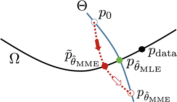

  

  Reprinted with permission from [184]. The blue curve illustrates the model distributions corresponding to different values of parameter θ. The black curve illustrates all the distributions that match p_data (black dot) in terms of E[h(x)]. The MLE $p_{\hat {\theta }_{\mathrm {MLE}}}$ (green dot) is the intersection between Θ (blue curve) and Ω (black curve). The MCMC (red dotted line) starts from p₀ (hollow blue dot) and runs toward $p_{\hat {\theta }_{\mathrm {MME}}}$ (hollow red dot), but the MCMC stops after K step, reaching $\tilde {p}_{\hat {\theta }_{\mathrm {MME}}}$ (red dot), which is the learned short-run MCMC

Thus even if the learned p_θ may be biased from MLE, the resulting short-run MCMC $\tilde {p}_\theta$ can nonetheless be considered a valid model, in that it matches p_data in terms of expectations of ∇_θf_θ(x). Recall in the case of FRAME model where f_θ(x) = 〈θ, h(x)〉, ∇_θf_θ(x) = h(x), i.e., the learned short-run MCMC $\tilde {p}_\theta$ matches p_data in terms of expectations of h(x). In general, ∇_θf_θ(x) may be considered a generalized version of feature vector h(x). Thus we may justify the learned short-run MCMC $\tilde {p}_\theta$ as a generalized moment matching estimator $\hat {\theta }_{\mathrm {MME}}$. The generalized moment matching explains the synthesis ability of the descriptive model and various learning schemes in general.

The short-run Langevin dynamics can be considered a noise-injected RNN or noise-injected residual network. Specifically, we can write x_K = F(x₀, e), where e = (e_k, k = 1, …, K). We can use it to reconstruct the observed image x by minimizing ∥x − F(x₀, e)∥ over x₀ and e. As a simple approximation, we can set e_k = 0 and write x_K = F(x₀) (Figs. 12.6 and 12.7).

Fig. 12.6

Reprinted with permission from [184]. Interpolation by short-run MCMC resembling a generator or flow model: The transition depicts the sequence F(z_ρ) with interpolated noise $z_\rho = \rho z_1 + \sqrt {1-\rho ^2} z_2$, where ρ ∈ [0, 1] on CelebA (64 × 64). Left: F(z₁). Right: F(z₂)

Fig. 12.7

Reprinted with permission from [184]. Reconstruction by short-run MCMC resembling a generator or flow model: The transition depicts F(z_t) over time t from random initialization t = 0 to reconstruction t = 200 on CelebA (64 × 64). Left: Random initialization. Right: Observed examples

12.2.9 Flow-Based Model

A flow-based model is of the form

$$\displaystyle \begin{aligned} x = g_\alpha(z); \; z \sim q_0(z), \end{aligned} $$

(12.31)

where q₀ is a known noise distribution. g_α is a composition of a sequence of invertible transformations where the log determinants of the Jacobians of the transformations can be explicitly obtained. α denotes the parameters. Let q_α(x) be the probability density of the model at a data point x with parameter α. Then under the change of variables, q_α(x) can be expressed as

$$\displaystyle \begin{aligned} q_\alpha(x) = q_0(g_\alpha^{-1}(x))|\det(\partial g_\alpha^{-1}(x)/\partial x)|. \end{aligned} $$

(12.32)

More specifically, suppose g_α is composed of a sequence of transformations $g_\alpha = g_{\alpha _1} \circ \cdots \circ g_{\alpha _m}$. The relation between z and x can be written as z ↔ h₁ ↔⋯ ↔ h_m−1 ↔ x. And thus we have

$$\displaystyle \begin{aligned} q_\alpha(x) = q_0(g_\alpha^{-1}(x)) \Pi_{t=1}^m |\det(\partial h_{t-1} / \partial h_t)|, \end{aligned} $$

(12.33)

where we define and for conciseness. With carefully designed transformations, as explored in flow-based methods, the determinant of the Jacobian matrix (∂h_t−1∕∂h_t) can be computed exactly. The key idea is to choose transformations whose Jacobian is a triangle matrix so that the determinant becomes

$$\displaystyle \begin{aligned} |\det(\partial h_{t-1} / \partial h_t)| = \Pi|{\mathrm{diag}}(\partial h_{t-1} / \partial h_{t})|. \end{aligned} $$

(12.34)

The following are the two scenarios for estimating q_α:

• (1) Generative modeling by MLE [13, 43, 44, 82, 131, 139, 233], by min_αD_KL (p_data∥q_α), where ${\mathrm {E}}_{p_{\mathrm {data}}}$ can be approximated by average over observed examples.

• (2) Variational approximation to an unnormalized target density p [130, 132, 202], based on min_αD_KL(q_α∥p), where

  $$\displaystyle \begin{aligned} \begin{array}{rcl} D_{\mathrm{KL}} (q_\alpha\|p) & =&\displaystyle {\mathrm{E}}_{q_\alpha}[\log q_\alpha(x)] - {\mathrm{E}}_{q_\alpha}[\log p(x)] \\ & =&\displaystyle {\mathrm{E}}_{z} [\log q_0(z) {-} \log |{\mathrm{det}}(g_\alpha^{\prime}(z))|] {-} {\mathrm{E}}_{q_\alpha}[\log p(x)]. \end{array} \end{aligned} $$

  (12.35)

  D_KL(q_α∥p) is the difference between energy and entropy, i.e., we want q_α to have low energy but high entropy. D_KL(q_α∥p) can be calculated without inversion of g_α.

When q_α appears on the right of KL-divergence, as in (1), it is forced to cover most of the modes of p_data. When q_α appears on the left of KL-divergence, as in (2), it tends to chase the major modes of p while ignoring the minor modes.

The flow-based model has explicit normalized density and can be sampled directly. It is both a density and a sampler.

12.2.10 Flow-Based Reference and Latent Space Sampling

[181] propose to use a flow-based model as the reference distribution for the descriptive model or the energy-based model (EBM) and perform MCMC sampling in latent space.

Instead of using uniform or Gaussian white noise distribution for the reference distribution q(x) in the descriptive model, we can use a flow-based model q_α as the reference model. q_α can be pre-trained by MLE and serves as the backbone of the model so that the model is of the following form:

$$\displaystyle \begin{aligned} p_\theta(x) = \frac{1}{Z(\theta)}\exp(f_\theta(x))q_\alpha(x). {} \end{aligned} $$

(12.36)

The resulting model p_θ(x) is a correction or refinement of q_α or an exponential tilting of q_α(x), and f_θ(x) is a free-form ConvNet to parameterize the correction. The overall negative energy is $f_\theta (x) + \log q_\alpha (x)$.

In the latent space of z, let p(z) be the distribution of z under p_θ(x); then

$$\displaystyle \begin{aligned} p(z) dz = p_\theta(x) dx = \frac{1}{Z(\theta)}\exp(f_\theta(x))q_\alpha(x) dx. \end{aligned} $$

(12.37)

Because q_α(x)dx = q₀(z)dz, we have

$$\displaystyle \begin{aligned} p(z) = \frac{1}{Z(\theta)}\exp(f_\theta(g_\alpha(z)))q_0(z). {} \end{aligned} $$

(12.38)

p(z) is an exponential tilting of the prior noise distribution q₀(z). It is a very simple form that does not involve the Jacobian or inversion of g_α(z).

Instead of sampling p_θ(x), we can sample p(z) in Eq. (12.38). While q_α(x) is multi-modal, q₀(z) is unimodal. Since p_θ(x) is a correction of q_α, p(z) is a correction of p₀(z) and can be much less multi-modal than p_θ(x) that is in the data space. After sampling z from p(z), we can generate x = g_α(z).

The above MCMC sampling scheme is a special case of neutral transport MCMC proposed by Hoffman et al. [104] for sampling from an EBM or the posterior distribution of a generative model. The basic idea is to train a flow-based model as a variational approximation to the target EBM and sample the EBM in the latent space of the flow-based model. In our case, since p_θ is a correction of q_α, we can simply use q_α directly as the approximate flow-based model in the neural transport sampler. The extra benefit is that the distribution p(z) is of an even simpler form than p_θ(x) because p(z) does not involve the inversion and Jacobian of g_α. As a result, we may use a flow-based backbone model of a more free form such as one based on residual network [13]. We use HMC [179] to sample from p(z) and push the samples forward to the data space through g_α. We can then learn θ by MLE.

12.2.11 Diffusion Recovery Likelihood

Inspired by recent work on diffusion-based models [102, 222, 223], [72] propose a diffusion recovery likelihood method to tackle the challenge of training the descriptive models or energy-based models (EBMs) directly on a dataset by instead learning a sequence of EBMs for the marginal distributions of the diffusion process. Specifically, assume a sequence of noisy observations x₀, x₁, …, x_T such that

$$\displaystyle \begin{aligned} \begin{array}{rcl} {\mathbf{x}}_0 \sim p_{\mathrm{data}}({\mathbf{x}});\;\; {\mathbf{x}}_{t+1} {=} \sqrt{1 {-} \sigma_{t+1}^2} {\mathbf{x}}_{t} {+} \sigma_{t+1} {\epsilon}_{t+1},\;\; t {=} 0, 1,\ldots T{-}1. {} \end{array} \end{aligned} $$

(12.39)

The scaling factor $\sqrt {1 - \sigma _{t+1}^2}$ ensures that the sequence is a spherical interpolation between the observed sample and Gaussian white noise. Let ${\mathbf {y}}_{t} = \sqrt {1 - \sigma _{t+1}^2} {\mathbf {x}}_{t}$, and we assume a sequence of marginal EBMs on the perturbed data

$$\displaystyle \begin{aligned} \begin{array}{rcl} p_\theta({\mathbf{y}}_t) = \frac{1}{Z_{\theta, t}} \exp\left(f_\theta({\mathbf{y}}_t, t)\right), {} \end{array} \end{aligned} $$

(12.40)

where f_θ(y_t, t) is defined by a neural network conditioned on t. The sequence of marginal EBMs can be learned with recovery likelihoods that are defined as the conditional distributions that invert the diffusion process, which can be derived by Eqs. (12.39) and (12.40):

$$\displaystyle \begin{aligned} p_\theta({\mathbf{y}}_{t}|{\mathbf{x}}_{t+1}) = \frac{1}{\tilde{Z}_{\theta, t}({\mathbf{x}}_{t+1})} \exp\left(f_\theta({\mathbf{y}}_{t}, t) - \frac{1}{2\sigma_{t+1}^2} \|{\mathbf{x}}_{t+1}-{\mathbf{y}}_t\|{}^2\right), \;\; t = 0, 1, \ldots, T-1. {} \end{aligned} $$

(12.41)

Compared to the standard maximum likelihood estimation (MLE) of EBMs, learning marginal EBMs by diffusion recovery likelihood only requires sampling from the conditional distributions in Eq. (12.41), which is much easier than sampling from the marginal distributions due to the additional quadratic term, which makes the conditional EBMs close to unimodal. After learning the marginal EBMs, we can generate synthesized images by a sequence of conditional samples initialized from the Gaussian white noise distribution using MCMC techniques such as Langevin sampling:

$$\displaystyle \begin{aligned} \begin{array}{rcl} {\mathbf{y}}^{\tau+1}_t = {\mathbf{y}}^{\tau}_t + \frac{b^2\sigma_t^2}{2} (\nabla_{\mathbf{y}} f_\theta({\mathbf{y}}^\tau_t, t) + \frac{1}{\sigma_t^2} ({\mathbf{x}}_{t+1}-{\mathbf{y}}_t^\tau)) + b \sigma_t {\epsilon}^\tau. {} \end{array} \end{aligned} $$

(12.42)

The framework of recovery likelihood was originally proposed in [17]. Gao et al. [72] adapt it to learning the sequence of marginal EBMs from the diffusion data. Figure 12.8 shows an illustration on a 2D toy example. Figure 12.9 displays uncurated samples generated from learned models on large image datasets.

Fig. 12.8

Reprinted with permission from [72]. Illustration of diffusion recovery likelihood on 2D checkerboard example. Top: progressively generated samples. Bottom: estimated marginal densities

Fig. 12.9

Reprinted with permission from [72]. Generated samples on LSUN 128² church_outdoor (left), LSUN 128² bedroom (center), and CelebA 64² (right)

12.2.12 Diffusion-Based Model

Diffusion-based models [102, 222, 223] prove to be exceedingly powerful in generating photorealistic images. It learns a sampling process instead of an explicit density. Thus it is on the side of the sampler (like a policy network), instead of density (like a value network). The sampling process is similar to the short-run Langevin dynamics for sampling from an energy-based model.

The key idea of the diffusion-based model of [222] is to continuously add noises of infinitesimal variance to the clean image until the resulting image becomes a Gaussian white noise image. This is a forward diffusion process. Then we learn to reverse this forward process by going from the Gaussian white noise distribution back to the multi-modal data distribution of the clean images. This reverse diffusion process is as if showing the movie of the forward diffusion process in reverse time, and it was inspired by the non-equilibrium thermodynamics [222]. The reverse diffusion process is a denoising process. Adding noises amounts to reducing the precision of the pixel intensities.

There are two slightly different perspectives on the diffusion-based model. One is based on the observation that the conditional distribution p_θ(y_t|x_t+1) in Eq. (12.41) is approximately Gaussian if $\sigma _{t+1}^2$ is infinitesimally small. The conditional Gaussian distribution can be derived by the first-order Taylor expansion of the log density of y_t. Thus the reverse process can be decomposed into a Markov sequence of conditional Gaussian models with infinitesimal variances, and they can be learned within the maximum likelihood or variational inference framework. A single conditional Gaussian model can be learned for the whole reverse process, with time embedding being input to the model. In the learning of the conditional Gaussian model, we can condition on the original clean image for the purpose of variance reduction. More specifically, at each time step of the diffusion process, we can predict the noise image that has been added to the original clean image, and then we can move toward the clean image by removing a small amount of the predicted noise image.

A closely related perspective is to estimate the derivative of the log density of the noisy image at each time step of the diffusion process by score matching [114, 115] via denoising auto-encoder [6, 227, 241]. The derivative of the log density or score is related to the first-order Taylor expansion mentioned above. The derivative or the score enables us to reverse the forward diffusion process via a stochastic differential equation [223].

Intuitively, for a population of points that follow a certain density, if we add small random noise to each point, the resulting population of perturbed points will have a density that is more diffused than the original density. We can achieve the same effect by perturbing each point deterministically via a gradient descent movement on the log density so that the resulting population of the deterministically perturbed points will have the same diffused density resulting from adding random noises. Thus we can reverse the effect of the noise diffusion by deterministic gradient ascent on the log density. This underlies the reversion of the forward diffusion process mentioned above. It also underlies the Langevin dynamics where the gradient ascent and the diffusion term balance each other.

The diffusion-based model is effective for modeling multi-modal data density by the reverse diffusion process starting from a unimodal Gaussian white noise density. The idea is related to simulated annealing [135], simulated tempering [168], parallel tempering [48, 77], or replica exchange [226] for sampling from multi-modal densities.

12.3 Equivalence Between Discriminative and Descriptive Models

12.3.1 Discriminative Model

Let x be an input example, e.g., an image or a text, and let y be a label or annotation of x, e.g., the category that x belongs to in the case of classification. Let us focus on the classification problem, and suppose there are C categories. The commonly used soft-max classifier assumes that

$$\displaystyle \begin{aligned} \begin{array}{rcl} p_\theta(y=c |x) = \frac{\exp(f_{c, \theta}(x))} {\sum_{c^{\prime} = 1}^{C} \exp(f_{c^{\prime}, \theta}(x))}, \end{array} \end{aligned} $$

(12.43)

where f_c,θ is a deep network, and θ denotes all the weight and bias parameters. For different c, the networks f_c,θ may share a common body and only differ in the head layer.

We can write the above model as

$$\displaystyle \begin{aligned} \begin{array}{rcl} p_\theta(y=c |x) = \frac{1}{Z(\theta)(x)} \exp(f_{c, \theta}(x)), \end{array} \end{aligned} $$

(12.44)

where

$$\displaystyle \begin{aligned} \begin{array}{rcl} Z(\theta)(x) = {\sum_{c= 1}^{C} \exp(f_{c, \theta}(x))}. \end{array} \end{aligned} $$

(12.45)

The discriminative model p_θ(y|x) can be learned by maximum likelihood. The log-likelihood is the average of

$$\displaystyle \begin{aligned} \begin{array}{rcl} \log p_\theta(y|x) = f_{y, \theta}(x) - \log Z(\theta)(x), \end{array} \end{aligned} $$

(12.46)

where the average is over the training set {x, y}. The gradient of $\log p_\theta (y|x)$ with respect to θ is

$$\displaystyle \begin{aligned} \begin{array}{rcl} \nabla_\theta \log p_\theta(y|x) = \nabla_\theta f_{y, \theta}(x) - {\mathrm{E}}_{p_\theta(y|x)} [ \nabla_\theta f_{y, \theta}(x)], \end{array} \end{aligned} $$

(12.47)

where

$$\displaystyle \begin{aligned} \begin{array}{rcl} \nabla_\theta \log Z(\theta)(x) = {\mathrm{E}}_{p_\theta(y|x)}[\nabla_\theta f_{y, \theta}(x)]. \end{array} \end{aligned} $$

(12.48)

Let p_data(x, y) be the data distribution of (x, y). The MLE minimizes D_KL(p_data(y|x)∥p_θ(y|x)), where for two conditional distributions p(y|x) and q(y|x), their KL-divergence is defined as

$$\displaystyle \begin{aligned} \begin{array}{rcl} D_{\mathrm{KL}}(p(y|x) \| q(y|x)) = {\mathrm{E}}_{p(x, y)} \left[ \log \frac{p(y|x)}{q(y|x)}\right], \end{array} \end{aligned} $$

(12.49)

where the expectation is with respect to p(x, y) = p(x)p(y|x), i.e., we also average over p(x) in addition to p(y|x).

The above calculations are analogous to the calculations for the descriptive model. The difference is that for the discriminative model, the normalizing constant Z and the expectation are summations over y, where y belongs to a finite set of categories, whereas for the descriptive model, the normalizing constant Z and the expectation are integral over x, where x belongs to a high-dimensional space. As a result, the expectation in the descriptive model cannot be calculated in closed form and has to be approximated by MCMC sampling such as Langevin dynamics.

A special case is binary classification, where y ∈{0, 1}. It is usually assumed that

$$\displaystyle \begin{aligned} \begin{array}{rcl} f_{0, \theta}(x) = 0, \; f_{1, \theta}(x) = f_\theta(x), \end{array} \end{aligned} $$

(12.50)

so that

$$\displaystyle \begin{aligned} \begin{array}{rcl} p_\theta(y = 1|x) = \frac{1}{1+ \exp(-f_\theta(x))} = {\mathrm{sigmoid}}(f_\theta(x)), \end{array} \end{aligned} $$

(12.51)

and y follows a nonlinear logistic regression on x.

12.3.2 Descriptive Model as Exponential Tilting of a Reference Distribution

A more general version of the descriptive model is of the following form of exponential tilting of a reference distribution [32, 253]:

$$\displaystyle \begin{aligned} \begin{array}{rcl} {} p_\theta(x) = \frac{1}{Z(\theta)} \exp(f_\theta(x)) q(x), \end{array} \end{aligned} $$

(12.52)

where q(x) is a given reference measure, such as uniform measure or Gaussian white noise distribution. The original form of the descriptive model corresponds to q(x) being a uniform measure. If q(x) is a Gaussian white noise distribution, then the energy function is − f_θ(x) + ∥x∥²∕2.

Although q(x) is usually taken to be a simple known distribution, q(x) can also be a model in its own right. We may call it a base model or a backbone model, and p_θ(x) can be considered a correction of q(x), where f_θ(x) is the correction term. We may also call p_θ(x) the energy-based correction of the base model q(x).

12.3.3 Discriminative Model via Bayes Rule

The above exponential tilting leads to the following discriminative model. We can treat p_θ as the positive distribution, and q(x) the negative distribution. Let y ∈{0, 1}, and the prior probability p(y = 1) = ρ, so that p(y = 0) = 1 − ρ. Let p(x|y = 1) = p_θ(x), p(x|y = 0) = q(x). Then according to the Bayes rule [32, 121, 143, 149, 234, 253],

$$\displaystyle \begin{aligned} \begin{array}{rcl} p(y = 1|x) = \frac{\exp(f_\theta(x) + b)}{1 + \exp(f_\theta(x)+b)}, \end{array} \end{aligned} $$

(12.53)

where $b = \log (\rho /(1-\rho )) - \log Z(\theta )$. This leads to nonlinear logistic regression. Sometimes, people call f_θ(x) + b the logit or logit score because

$$\displaystyle \begin{aligned} \begin{array}{rcl} \log \frac{p(y=1|x)}{p(y=0|x)} = {\mathrm{logit}}(p(y=1|x)) = f_\theta(x) + b. \end{array} \end{aligned} $$

(12.54)

More generally, suppose we have C categories, and

$$\displaystyle \begin{aligned} \begin{array}{rcl} p_{c, \theta}(x) = \frac{1}{Z_{c, \theta}} \exp(f_{c, \theta}(x)) q(x), \; c = 1, \ldots, C, \end{array} \end{aligned} $$

(12.55)

where (f_c,θ(x), c = 1, …, C) are C networks that may share the same body but with different heads. Suppose the prior probability for category c is ρ_c, then

$$\displaystyle \begin{aligned} \begin{array}{rcl} p(y = c | x) = \frac{\exp(f_{c, \theta}(x) + b_c)}{\sum_{c=1}^{C} \exp(f_{c, \theta}(x) + b_c)}, \end{array} \end{aligned} $$

(12.56)

where $b_c = \log \rho _c - \log Z_{c, \theta }$. The above is a conventional soft-max classifier. Conversely, if p(y = c|x) is of the above form of soft-max classifier, then p_c,θ(x) is of the form of exponential tilting based on the logit score f_c,θ(x) + b_c. Thus the discriminative model and the descriptive model are equivalent to each other.

12.3.4 Noise Contrastive Estimation

The above equivalence suggests that we can learn the descriptive model by fitting a logistic regression. Specifically, suppose we want to learn a descriptive model $p_\theta (x) = \frac {1}{Z(\theta )} \exp (f_\theta (x)) q(x)$, where q(x) is a noise distribution, such as Gaussian white noise distribution. We can treat the observed examples as the positive examples, so that for each positive x, y = 1, and we generate negative examples from the noise distribution q(x), so that for each negative example x ∼ q(x), y = 0. Then we learn a discriminator in the form of logistic regression to distinguish between the positive and negative examples, and then logit(p(y = 1|x)) = f_θ(x) + b, where $b = \log (\rho /(1-\rho )) - \log Z(\theta )$, where ρ is the proportion of the positive examples. We can learn both θ and b by fitting a logistic regression, where b is treated as an independent bias or intercept term, even though $\log Z(\theta )$ depends on θ. This enables us to learn f_θ and estimate $\log Z(\theta )$. This is called noise contrastive estimation (NCE) [92].

The problem with the above scheme is that the noise distribution and the data distribution usually do not have much overlap, especially if x is of high dimensionality. As a result, f_θ(x) cannot be well learned.

The introspective learning method [121, 234] tries to remedy the above problem with sampling. After learning f_θ(x) by noise contrastive estimation, we want to inspect whether f_θ(x) is well learned. We then treat the current p_θ(x) as our new q(x), and we draw negative samples from it. If it is well learned, then the negative samples will be close to the positive examples. To check that, we fit a logistic regression again on the positive examples and negative examples from the new q(x). Then we learn a new Δf_θ(x) by the new logistic regression. This Δf_θ(x) can then be added to the previous learned f_θ(x) to obtain the new f_θ(x). We can keep repeating this process until Δf_θ(x) is small.

In general, while the descriptive model learns the probability density function, the discriminative model learns the ratios between the probability densities of different classes. If we know the density of a base class, such as the Gaussian white noise, we can learn the densities of other classes by noise contrastive estimation. Noise contrastive estimation is a form of self-supervised learning.

Noise contrastive estimation (NCE) based on diffusion sequence is explored in [203].

12.3.5 Flow Contrastive Estimation

Gao et al. [71] propose an improvement of noise contrastive estimation (NCE) [92] based on the flow-based model. The basic idea is to transform the noise so that the resulting distribution is closer to the data distribution. This is exactly what the flow model achieves. That is, a flow model transforms a known noise distribution q₀(z) by a composition of a sequence of invertible transformations g_α(⋅). However, in practice, we find that a pre-trained q_α(x), such as learned by MLE, is not strong enough for learning an EBM p_θ(x) because the synthesized data from the MLE of q_α(x) can still be easily distinguished from the real data by an EBM. Thus, we propose to iteratively train the EBM and flow model, in which case the flow model is adaptively adjusted to become a stronger contrast distribution or a stronger training opponent for EBM. This is achieved by a parameter estimation scheme similar to GAN [81, 199], where p_θ(x) and q_α(x) play a minimax game with a unified value function: min_αmax_θV (θ, α),

$$\displaystyle \begin{aligned} \begin{array}{rcl} V(\theta, \alpha) = {\mathrm{E}}_{p_{\mathrm{data}}} \left[ \log \frac{p_\theta(x)}{p_\theta(x) + q_\alpha(x)}\right] + {\mathrm{E}}_{z}\left[\log \frac{q_\alpha(g_\alpha(z))}{p_\theta(g_\alpha(z)) + q_\alpha(g_\alpha(z))}\right], {}\\ \end{array} \end{aligned} $$

(12.57)

where ${\mathrm {E}}_{p_{\mathrm {data}}}$ is approximated by averaging over observed samples {x_i, i = 1, …, n}, while E_z is approximated by averaging over negative samples $\{\tilde {x}_i, i = 1,\ldots ,n\}$ drawn from q_α(x), with z_i ∼ q₀(z) independently for i = 1, …, n. In the experiments, we choose Glow [131] as the flow-based model. The algorithm can start from either a randomly initialized Glow model or a pre-trained one by MLE. Here we assume equal prior probabilities for observed samples and negative samples. It can be easily modified to the situation where we assign a higher prior probability to the negative samples, given the fact we have access to an infinite amount of free negative samples.

The objective function can be interpreted from the following perspectives:

• (1) Noise contrastive estimation for EBM. The update of θ can be seen as noise contrastive estimation of p_θ(x), but with a flow-transformed noise distribution q_α(x) that is adaptively updated. The training is essentially a logistic regression. However, unlike regular logistic regression for classification, for each x_i or $\tilde {x}_i$, we must include $\log q_\alpha (x_i)$ or $\log q_\alpha (\tilde {x}_i)$ as an example-dependent bias term. This forces p_θ(x) to replicate q_α(x) in addition to distinguishing between p_data(x) and q_α(x), so that p_θ(x_i) is in general larger than q_α(x_i), and $p_\theta (\tilde {x}_i)$ is in general smaller than $q_\alpha (\tilde {x}_i)$.

• (2) Minimization of Jensen–Shannon divergence for the flow model. If p_θ(x) is close to the data distribution, then the update of α is approximately minimizing the Jensen–Shannon divergence between the flow model q_α and data distribution p_data:

  $$\displaystyle \begin{aligned} D_{\mathrm{JS}}(q_\alpha \| p_{\mathrm{data}})=D_{\mathrm{KL}}(p_{\mathrm{data}} \| (p_{\mathrm{data}} + q_\alpha)/2) + D_{\mathrm{KL}}(q_\alpha \| (p_{\mathrm{data}} + q_\alpha)/2). \end{aligned} $$

  (12.58)

  Its gradient w.r.t. α equals the gradient of $-{\mathrm {E}}_{p_{\mathrm {data}}}[\log ((p_\theta + q_\alpha )/2)] + D_{\mathrm {KL}}(q_\alpha \| (p_\theta + q_\alpha )/2)$. The gradient of the first term resembles MLE, which forces q_α to cover the modes of data distribution, and tends to lead to an over-dispersed model, which is also pointed out in [131]. The gradient of the second term is similar to reverse Kullback–Leibler divergence between q_α and p_θ, or variational approximation of p_θ by q_α, which forces q_α to chase the modes of p_θ. This may help correct the over-dispersion of MLE.

• (3) Connection with GAN [81, 199]. Our parameter estimation scheme is closely related to GAN. In GAN, the discriminator D and generator G play a minimax game: min_Gmax_DV (G, D),

  $$\displaystyle \begin{aligned} V(G, D) = {\mathrm{E}}_{p_{\mathrm{data}}} \left[ \log D(x)\right] + {\mathrm{E}}_z\left[ \log(1 - D(G(z_i)))\right]. \end{aligned} $$

  (12.59)

  The discriminator D(x) is learning the probability ratio p_data(x)∕(p_data(x) + p_G(x)), which is about the difference between p_data and p_G [56]. p_G is the density of the generated data. In the end, if the generator G learns to perfectly replicate p_data, then the discriminator D ends up with a random guess. However, in our method, the ratio is explicitly modeled by p_θ and q_α. p_θ must contain all the learned knowledge in q_α, in addition to the difference between p_data and q_α. In the end, we learn two explicit probability distributions p_θ and q_α as approximations to p_data.

12.4 Generative Latent Variable Model

12.4.1 Model and Origin

Both discriminative model and descriptive model are based on a bottom-up network f_θ(x). The generative model is based on top-down network with latent variables. The prototype of such a model is factor analysis. Let x be the observed example, which is a D-dimensional vector. We assume that x can be explained by a d-dimensional latent vector, each element of which is called a factor. Given z, x is generated by x = Wz + 𝜖, where W is a D × d matrix, sometimes called loading matrix. It is usually assumed that z ∼N(0, I_d), where I_d is d-dimensional identity matrix, 𝜖 ∼N(0, σ²I_D), and 𝜖 is independent of z. The factor analysis model originated from psychometrics, where x consists of a pupil’s scores on a number of subjects, and z = (z₁, z₂), where z₁ is verbal intelligence and z₂ is analytical intelligence.

A recent generalization [81, 133] is to keep the prior assumption about z, but replace the linear model x = Wz + 𝜖 by a nonlinear model x = g_θ(z) + 𝜖, where g_θ(z) is parameterized by a top-down neural network where θ collects all the weight and bias parameters. In the case of image modeling, g_θ(z) is usually a convolutional neural network, which is sometimes called deconvolutional network, due to its top-down nature. The above model leads to a conditional or generation model p_θ(x|z), such that

$$\displaystyle \begin{aligned} \log p_\theta(x, z) &= \log [p(z) p_\theta(x|z) ] \end{aligned} $$

(12.60)

$$\displaystyle \begin{aligned} &= -\frac{1}{2} \left[ \|z\|{}^2 + \|x - g_\theta(z)\|{}^2/\sigma^2\right] + c, {} \end{aligned} $$

(12.61)

where c is a constant independent of θ. σ² is usually treated as a tuning parameter. The model follows the manifold assumption, which assumes that the density of the D-dimensional data focuses on a lower, d-dimensional manifold.

The joint distribution of (x, z) is p_θ(x, z) = p(z)p_θ(x|z). The marginal distribution of x is $p_\theta (x) = \int p_\theta (x, z) dz.$ The marginal distribution is analytically intractable due to the integration of z. The model specifies a direct sampling method for generating x, but it does not explicitly specify the density of x.

Given x, the inference of z can be based on the posterior distribution p_θ(z|x) = p_θ(x, z)∕p_θ(x), which is also intractable due to the intractability of the marginal p_θ(x).

The above model is often referred to as the generator network in the literature.

12.4.2 Generative Model with Multi-layer Latent Variables

While it is computationally convenient to have a single latent noise vector at the top layer, it does not account for the fact that patterns can appear at multiple layers of compositions or abstractions (e.g., face → (eyes, nose, mouth) → (edges, corners) → pixels), where variations and randomness occur at multiple layers. To capture such a hierarchical structure, it is desirable to introduce multiple layers of latent variables organized in a top-down architecture [183]. Specifically, we have z = (z_l, l = 1, …, L), where layer L is the top layer, and layer 1 is the bottom layer above x. For notational simplicity, we let x = z₀. We can then specify p_θ(z) as

$$\displaystyle \begin{aligned} p_{\theta}(z) = p_{\theta}(z_L) \prod_{l=0}^{L-1}p_{\theta}(z_l | z_{l+1}). \end{aligned} $$

(12.62)

One concrete example is z_L ∼N(0, I), $[z_l|z_{l+1}] \sim {\mathrm {N}}(\mu _l(z_{l+1}), \sigma _l^2(z_{l+1})), \; l = 0, \ldots , L-1$, where μ_l() and $\sigma _l^2()$ are the mean vector and the diagonal variance–covariance matrix of z_l, respectively, and they are functions of z_l+1. θ collects all the parameters in these functions. p_θ(x, z) can be obtained similarly as in Eq. (12.61).

12.4.3 MLE Learning and Posterior Inference

Let p_data(x) be the data distribution that generates the example x. The learning of parameters θ of p_θ(x) can be based on min_θD_KL(p_data(x)∥p_θ(x)). If we observe training examples {x_i, i = 1, …, n}∼ p_data(x), the above minimization can be approximated by maximizing the log-likelihood

$$\displaystyle \begin{aligned} L(\theta) = \frac{1}{n} \sum_{i=1}^{n} \log p_\theta(x_i) \doteq {\mathrm{E}}_{{p_{\mathrm{data}}}}[\log p_\theta(x)], \end{aligned} $$

(12.63)

which leads to MLE.

The gradient of the log-likelihood, L^′(θ), can be computed according to the following identity:

$$\displaystyle \begin{aligned} \delta_\theta(x) &= \nabla_\theta \log p_\theta(x) = \frac{1}{p_\theta(x)} \nabla_\theta p_\theta(x) \end{aligned} $$

(12.64)

$$\displaystyle \begin{aligned} & = \frac{1}{p_\theta(x)} \int \nabla_\theta p_\theta(x, z) dz \end{aligned} $$

(12.65)

$$\displaystyle \begin{aligned} &= {\mathrm{E}}_{p_\theta(z|x)} \left[ \nabla_\theta \log p_\theta(x, z)\right]. \end{aligned} $$

(12.66)

Thus

$$\displaystyle \begin{aligned} L^{\prime}(\theta) = {\mathrm{E}}_{{p_{\mathrm{data}}}}[\delta_\theta(x)] &= {\mathrm{E}}_{{p_{\mathrm{data}}}(x)} {\mathrm{E}}_{p_{\theta}(z|x)}\left[ \nabla_\theta \log p_{\theta}(x, z) \right] \end{aligned} $$

(12.67)

$$\displaystyle \begin{aligned} &\doteq \frac{1}{n} \sum_{i=1}^{n} {\mathrm{E}}_{p_{\theta}(z_i|x_i)}\left[ \nabla_\theta \log p_{\theta}(x_i, z_i) \right]. \end{aligned} $$

(12.68)

The expectation with respect to p_θ(z|x) can be approximated by Monte Carlo samples. Each learning iteration updates θ by θ_t+1 = θ_t + η_tL^′(θ_t).

12.4.4 Posterior Sampling

Sampling from p_θ(z|x) usually requires MCMC. One convenient MCMC is Langevin dynamics, which iterates

$$\displaystyle \begin{aligned} z_{t+1} = z_t + s \nabla_z \log p_\theta(z_t|x) + \sqrt{2s} e_t, \end{aligned} $$

(12.69)

where e_t ∼N(0, I), t indexes the time step of the Langevin dynamics, and s is the step size. The Langevin dynamics consists of a gradient descent term on $-\log p(z|x)$. In the case of generator network, it amounts to gradient descent on ∥z∥²∕2 + ∥x − g_θ(z)∥²∕2σ², which is the penalized reconstruction error. The Langevin dynamics also consists of a white noise diffusion term $\sqrt {2s} e_t$ to create randomness for sampling from p_θ(z|x).

For small step size s, the marginal distribution of z_t will converge to p_θ(z|x) as t →∞ regardless of the initial distribution of z₀. More specifically, let p_t(z) be the marginal distribution of z_t of the Langevin dynamics, and then D_KL(p_t(z)∥p_θ(z|x)) decreases monotonically to 0, that is, by increasing t, we reduce D_KL(p_t(z)∥p_θ(z|x)) monotonically.

12.4.5 Perturbation of KL-divergence

Again we understand the MLE learning algorithm by perturbing the KL-divergence for MLE. Define D(θ) = D_KL(p_data∥p_θ). It is the objective function of MLE. Let θ_t be the estimate at iteration t. Let us consider the following perturbation of D(θ):

$$\displaystyle \begin{aligned} S(\theta) &= D(\theta) + D_{\mathrm{KL}}(p_{\theta_t}(z|x) \| p_\theta(z|x)) \end{aligned} $$

(12.70)

$$\displaystyle \begin{aligned} &= D_{\mathrm{KL}}({p_{\mathrm{data}}}(x) \| p_\theta(x)) + D_{\mathrm{KL}}(p_{\theta_t}(z|x) \| p_\theta(z|x)) \end{aligned} $$

(12.71)

$$\displaystyle \begin{aligned} &= D_{\mathrm{KL}}(p_{{\mathrm{data}}, \theta_t}(x, z) \| p_\theta(x, z)), \end{aligned} $$

(12.72)

where we define $p_{{\mathrm {data}}, \theta _t}(x, z) = p_{\mathrm {data}}(x) p_{\theta _t}(z|x)$. Again S(θ) is a surrogate for D(θ) at θ_t, and S(θ) is simpler than D(θ) because S(θ) is based on the joint distributions instead of the marginal distributions as in D(θ). Unlike the joint distribution p_θ(x, z) = p(z)p_θ(x|z), the marginal distribution $p_\theta (x) = \int p_\theta (x, z) dz$ is implicit as it is an intractable integral (Fig. 12.10).

Fig. 12.10

Reprinted with permission from [95]. The surrogate S majorizes (upper bounds) D, and they touch each other at θ_t with the same tangent

The perturbation term $D_{\mathrm {KL}}(p_{\theta _t}(z|x) \| p_\theta (z|x))$, as a function of θ, achieves its minimum 0 at θ = θ_t, and its derivative at θ = θ_t is zero. Thus S(θ) and D(θ) touch each other at θ_t, and they share the same gradient at θ_t.

$$\displaystyle \begin{aligned} \begin{array}{rcl} -S(\theta) = {\mathrm{E}}_{p_{\mathrm{data}}(x)} {\mathrm{E}}_{p_{\theta_t}(z|x)}[\log p_\theta(x, z)] - {\mathrm{entropy}}(p_{{\mathrm{data}}, \theta_t}(x, z)). \end{array} \end{aligned} $$

(12.73)

$$\displaystyle \begin{aligned} \begin{array}{rcl} - S^{\prime}(\theta) = {\mathrm{E}}_{p_{\mathrm{data}}(x)} {\mathrm{E}}_{p_{\theta_t}(z|x)}[\nabla_\theta \log p_\theta(x, z)]. \end{array} \end{aligned} $$

(12.74)

Thus, the learning gradient at θ_t is

$$\displaystyle \begin{aligned} -D^{\prime}(\theta_t) = - S^{\prime}(\theta_t) = {\mathrm{E}}_{{p_{\mathrm{data}}}}[\delta_{\theta_t}(x)] = {\mathrm{E}}_{p_{\mathrm{data}}(x)} {\mathrm{E}}_{p_{\theta_t}(z|x)}[\nabla_\theta \log p_{\theta_t}(x, z)]. \end{aligned} $$

(12.75)

This provides another justification for the learning algorithm.

The above perturbation of KL-divergence can be compared to that in the descriptive model, where the sign in front of the second KL-divergence is negative, in order to cancel the intractable $\log Z(\theta )$ term. For the generative model, the sign in front of the second KL-divergence is positive, in order to change the marginal distributions in the first KL-divergence, i.e., D(θ), into the joint distributions, so that p_θ(z, x) = p(z)p_θ(x|z) is obtained in closed form.

12.4.6 Short-Run MCMC for Approximate Inference

We can use short-run MCMC as inference dynamics [183], with a fixed small K (e.g., K = 25),

$$\displaystyle \begin{aligned} z_0 \sim p(z), z_{k+1} = z_k + s \nabla_z \log p_\theta(z_k|x) + \sqrt{2s} e_k, \; k = 1, \ldots, K, {} \end{aligned} $$

(12.76)

where p(z) is the prior noise distribution of z.

We can write the above short-run MCMC as

$$\displaystyle \begin{aligned} z_0 \sim p(z), \; z_{k+1} = z_k + s R(z_k) + \sqrt{2s} e_k, \; k = 1, \ldots, K, \end{aligned} $$

(12.77)

$R(z) = \nabla _z \log p_\theta (z|x)$, where we omit x and θ in R(z) for simplicity of notation.

To further simplify the notation, we may write the short-run MCMC as

$$\displaystyle \begin{aligned} z_0 \sim p(z), \; z_K = F(z_0, e), \end{aligned} $$

(12.78)

where e = (e_k, k = 1, …, K), and F composes the K steps of Langevin updates.

Let the distribution of z_K be $\tilde {p}(z)$. Recall that the distribution of z_K also depends on x and θ and step size s, so that in full notation, we may write $\tilde {p}(z)$ as $\tilde {p}_{s, \theta }(z|x)$.

For each x, we define

$$\displaystyle \begin{aligned} \begin{array}{rcl} \tilde{\delta}_\theta(x) = {\mathrm{E}}_{\tilde{p}_{s,\theta}(z|x)} \left[ \nabla_\theta \log p_\theta(x, z)\right] \end{array} \end{aligned} $$

(12.79)

and modify the learning algorithm to

$$\displaystyle \begin{aligned} \theta_{t+1} = \theta_t + \eta_t {\mathrm{E}}_{{p_{\mathrm{data}}}}[\tilde{\delta}_{\theta_t}(x)] = \theta_t + \eta_t E_{{p_{\mathrm{data}}}}{\mathrm{E}}_{\tilde{p}_{s, \theta_t}(z|x)} \left[ \nabla_\theta \log p_{\theta_t}(x, z)\right], \end{aligned} $$

(12.80)

where η_t is the learning rate and ${\mathrm {E}}_{\tilde {p}_{s, \theta _t}(z_i|x_i)}$ (here we use the full notation $\tilde {p}_{s, \theta }(z|x)$ instead of the abbreviated notation q(z)) can be approximated by sampling from $\tilde {p}_{s, \theta _t}(z_i|x_i)$ using the noise initialized K-step Langevin dynamics.

Compared to MLE learning algorithm, we replace p_θ(z|x) by $\tilde {p}_{s, \theta }(z|x)$, and fair Monte Carlo samples from $\tilde {p}_{s, \theta }(z|x)$ can be obtained by short-run MCMC.

One major advantage of the proposed method is that it is simple and automatic. For models with multiple layers of latent variables that may be organized in complex top-down architectures, the gradient computation in Langevin dynamics is automatic on modern deep learning platforms. Such dynamics naturally integrates explaining-away competitions and bottom-up and top-down interactions between multiple layers of latent variables. It thus enables researchers to explore flexible generative models without dealing with the challenging task of designing and learning the inference models. The short-run MCMC is automatic, natural, and biologically plausible as it may be related to attractor dynamics [7, 108, 198].

12.4.7 Objective Function and Estimating Equation

The following are justifications for learning with short-run MCMC:

• (1) Objective function. Again we use perturbation of KL-divergence. At iteration t, with θ_t fixed, the learning algorithm follows the gradient of the following perturbation of D(θ) at θ = θ_t:

  $$\displaystyle \begin{aligned} S(\theta) &= D(\theta) + D_{\mathrm{KL}}(\tilde{p}_{s, \theta_t}(z|x) \| p_\theta(z|x)) \end{aligned} $$

  (12.81)
  $$\displaystyle \begin{aligned} &= D_{\mathrm{KL}}({p_{\mathrm{data}}}(x)\|p_\theta(x)) + D_{\mathrm{KL}}(\tilde{p}_{s, \theta_t}(z|x)\|p_\theta(z|x)), \end{aligned} $$

  (12.82)

  so that θ_t+1 = θ_t − η_tS^′(θ_t), where η_t is the step size, and

  $$\displaystyle \begin{aligned} \begin{array}{rcl} -S^{\prime}(\theta) = {\mathrm{E}}_{p_{\mathrm{data}}(x)} {\mathrm{E}}_{\tilde{p}_{s,\theta_t}(z|x)}[\nabla_\theta \log p_\theta(x, z)]. \end{array} \end{aligned} $$

  (12.83)
  $$\displaystyle \begin{aligned} \begin{array}{rcl} -S^{\prime}(\theta_t) = {\mathrm{E}}_{{p_{\mathrm{data}}}}[\tilde{\delta}_{\theta_t}(x)] = {\mathrm{E}}_{p_{\mathrm{data}}(x)} {\mathrm{E}}_{\tilde{p}_{s, \theta_t}(z|x)}[\nabla_\theta \log p_{\theta_t}(x, z)]. \end{array} \end{aligned} $$

  (12.84)

  Compared to the perturbation of KL-divergence in MLE learning, we use $\tilde {p}_{s, \theta _t}(z|x)$ instead of $p_{\theta _t}(z|x)$. While sampling $p_{\theta _t}(z|x)$ can be impractical if it is multi-modal, sampling $\tilde {p}_{s, \theta _t}(z|x)$ is practical because it is a short-run MCMC.

• (2) Estimating equation. The fixed point of the learning algorithm (12.80) solves the following estimating equation:

  $$\displaystyle \begin{aligned} \frac{1}{n} \sum_{i=1}^{n} {\mathrm{E}}_{\tilde{p}_{s, \theta}(z_i|x_i)}\left[ \nabla_\theta \log p_{\theta}(x_i, z_i)\right] \doteq {\mathrm{E}}_{p_{\mathrm{data}}(x)} {\mathrm{E}}_{\tilde{p}_{s, \theta}(z|x)}\left[ \nabla_\theta \log p_{\theta}(x, z)\right] = 0. {} \end{aligned} $$

  (12.85)

  If we approximate ${\mathrm {E}}_{\tilde {p}_{s, \theta _t}(z_i|x_i)}$ by Monte Carlo samples from $\tilde {p}_{s, \theta _t}(z_i|x_i)$, then the learning algorithm becomes Robbins–Monro algorithm for stochastic approximation [205].

The bias of the learned θ based on short-run MCMC relative to the MLE depends on the gap between $\tilde {p}_{s, \theta }(z|x)$ and p_θ(z|x). We suspect that this bias may actually be beneficial in the following sense. The learning gradient seeks to decrease D(θ) while decreasing $D_{\mathrm {KL}} (\tilde {p}_{s, \theta _t}(z_i|x_i) \| p_{\theta }(z_i|x_i))$. The latter tends to bias the learned model so that its posterior distribution p_θ(z_i|x_i) is close to the short-run MCMC $\tilde {p}_{s, \theta _t}(z_i|x_i)$, i.e., our learning method may bias the model to make inference by short-run MCMC accurate.

We can optimize the step size s and other algorithmic parameters of the short-run Langevin dynamics by minimizing $D_{\mathrm {KL}} (\tilde {p}_{s, \theta _t}(z_i|x_i) \| p_{\theta }(z_i|x_i))$ over s. This is a variational optimization.

12.5 Descriptive Model in Latent Space of Generative Model

12.5.1 Top-Down and Bottom-Up

$$\displaystyle \begin{aligned} \begin{array}{rcl} \begin{array}[c]{ccc} \mbox{Top-down mapping} && \mbox{Bottom-up mapping}\\ \mbox{hidden vector }z && \mbox{energy }-f_\theta(x)\\ \Downarrow&&\Uparrow\\ \mbox{signal }x \approx g_\theta(z) && \mbox{signal }x \\ \mbox{(a) {Generator model} }&& \mbox{(b) Descriptive model} \end{array} {} \end{array} \end{aligned} $$

(12.86)

The above diagram compares the generative model and the descriptive model. The former is based on top-down generation, whereas the latter is based on the bottom-up description.

The top-down model is a very natural representation of knowledge, with its multiple layers of latent variables representing concepts at multiple levels of abstractions. The top-down model is also called the directed acyclic graphical model. It is characterized by independence or conditional independence assumptions of the latent variables. Such assumptions limit the expressive power of the top-down model.

For the special case of the generator network, there is a latent vector z at the top layer, which generates the example x via the top-down generation mapping g_θ(z). The prior distribution of z is usually assumed to be a simple noise distribution, e.g., the Gaussian white noise distribution z ∼N(0, I). The top-down g_θ(z) maps this simple isotropic unimodal prior distribution to the multi-modal data distribution p_data. However, the expressive power may be limited by the simple prior distribution p(z) (as well as the simple Gaussian white noise distribution of 𝜖 in x = g_θ(z) + 𝜖). The marginal distribution of $p_\theta (x) = \int p(z) p_\theta (x|z) dz$ is implicit because of the intractable integral over the latent z.

The bottom-up model only needs to specify a scalar-valued energy function − f_θ(x), instead of a vector-valued g_θ(z), while leaving the generative task to MCMC. It specifies the distribution $p_\theta (x) = \frac {1}{Z(\theta )} \exp (f_\theta (x))$ explicitly even though the normalizing constant Z(θ) is intractable. Compared to the generator model, the descriptive model tends to have stronger expressive power in terms of synthesis ability.

However, because p_data tends to be highly multi-modal, the learned p_θ can also be highly multi-modal. As a result, MCMC sampling cannot mix. Even though we can use short-run MCMC to learn the model and synthesize images, the model is admittedly biased. One remedy is to use more sophisticated MCMC such as parallel tempering [189] or replica exchange MCMC [226]. The other option is to move the descriptive model to the latent space.

12.5.2 Descriptive Energy-Based Model in Latent Space

We follow the philosophy of empirical Bayes, that is, instead of assuming a given prior distribution for the latent vector, as in the generator network, we learn a prior model from empirical observations.

Specifically, we assume the latent vector follows a descriptive model or, more specifically, an energy-based correction of the isotropic Gaussian white noise prior distribution. We call this model the latent space descriptive model. Such a model adds more expressive power to the generator model. In the latent space, the descriptive model is close to unimodal as it is a correction of the unimodal Gaussian distribution, and MCMC sampling is expected to mix well.

The MLE learning of the generative model with a latent space descriptive model involves MCMC sampling of the latent vector from both the prior and posterior distributions. Parameters of the prior model can then be updated based on the statistical difference between samples from the two distributions. Parameters of the top-down network can be updated based on the samples from the posterior distribution as well as the observed data.

Let $x \in \mathbb {R}^D$ be an observed example such as an image or a piece of text, and let $z \in \mathbb {R}^d$ be the latent variables, where D ≫ d. The joint distribution of (x, z) is

$$\displaystyle \begin{aligned} p_{\theta}(x, z) &= p_{\alpha}(z) p_\beta(x|z), \end{aligned} $$

(12.87)

where p_α(z) is the prior model with parameters α, p_β(x|z) is the top-down generation model with parameters β, and θ = (α, β).

The prior model p_α(z) is formulated as a descriptive model or an energy-based model

$$\displaystyle \begin{aligned} p_{\alpha}(z) = \frac{1}{Z(\alpha)} \exp(f_{\alpha}(z)) p_0(z), {} \end{aligned} $$

(12.88)

where p₀(z) is a reference distribution, assumed to be isotropic Gaussian white noise distribution. f_α(z) is the negative energy and is parameterized by a small multi-layer perceptron with parameters α. $Z(\alpha ) = \int \exp (f_\alpha (z)) p_0(z) dz = {\mathrm {E}}_{p_0}[\exp (f_\alpha (z))]$ is the normalizing constant or partition function.

The prior model (12.88) can be interpreted as an energy-based correction or exponential tilting of the original prior distribution p₀, which is the prior distribution in the generator model.

The generation model is the same as the top-down network in the generator model. For image modeling,

$$\displaystyle \begin{aligned} x = g_\beta(z) + \epsilon, \end{aligned} $$

(12.89)

where 𝜖 ∼N(0, σ²I_D), so that p_β(x|z) ∼N(g_β(z), σ²I_D). Usually, σ² takes an assumed value. For text modeling, let x = (x^(t), t = 1, …, T), where each x^(t) is a token. A commonly used model is to define p_β(x|z) as a conditional auto-regressive model,

$$\displaystyle \begin{aligned} p_\beta(x|z) = \prod_{t=1}^T p_\beta(x^{(t)}|x^{(1)}, \ldots, x^{(t-1)}, z), \end{aligned} $$

(12.90)

which is often parameterized by a recurrent network with parameters β.

In the original generator model, the top-down network g_β maps the unimodal prior distribution p₀ to be close to the usually highly multi-modal data distribution. The prior model in (12.88) refines p₀ so that g_β maps the prior model p_α to be closer to the data distribution. The prior model p_α does not need to be highly multi-modal because of the expressiveness of g_β.

The marginal distribution is $p_{\theta }(x) = \int p_\theta (x, z) dz = \int p_\alpha (z) p_\beta (x|z) dz.$ The posterior distribution is p_θ(z|x) = p_θ(x, z)∕p_θ(x) = p_α(z)p_β(x|z)∕p_θ(x).

In the above model, we exponentially tilt p₀(z). We can also exponentially tilt p₀(x, z) = p₀(z)p_β(x|z) to $p_\theta (x, z) = \frac {1}{Z(\theta )} \exp (f_\alpha (x, z)) p_0(x, z)$. Equivalently, we may also exponentially tilt p₀(z, 𝜖) = p₀(z)p(𝜖), as the mapping from (z, 𝜖) to (z, x) is a change of variable. This leads to a descriptive model in both the latent space and data space, which makes learning and sampling more complex. Therefore, we choose to only tilt p₀(z) and leave p_β(x|z) as a directed top-down generation model.

12.5.3 Maximum Likelihood Learning

Suppose we observe training examples (x_i, i = 1, …, n). The log-likelihood function is

$$\displaystyle \begin{aligned} L( \theta) = \frac{1}{n}\sum_{i=1}^{n} \log p_\theta(x_i) \doteq {\mathrm{E}}_{{p_{\mathrm{data}}}}[\log p_\theta(x)]. {} \end{aligned} $$

(12.91)

The learning gradient can be calculated according to

$$\displaystyle \begin{aligned} \nabla_\theta \log p_\theta(x) & = {\mathrm{E}}_{p_\theta(z|x)} \left[ \nabla_\theta \log p_\theta(x, z) \right] = {\mathrm{E}}_{p_\theta(z|x)} \left[ \nabla_\theta (\log p_\alpha(z) + \log p_\beta(x|z)) \right]. \end{aligned} $$

(12.92)

For the prior model, $\nabla _\alpha \log p_\alpha (z) = \nabla _\alpha f_\alpha (z) - {\mathrm {E}}_{p_\alpha (z)}[ \nabla _\alpha f_\alpha (z)].$ Thus the learning gradient for an example x is

$$\displaystyle \begin{aligned} \delta_\alpha(x) = \nabla_\alpha \log p_\theta(x) = {\mathrm{E}}_{p_\theta(z|x)}[\nabla_\alpha f_\alpha(z)] - {\mathrm{E}}_{p_\alpha(z)} [\nabla_\alpha f_\alpha(z)]. {} \end{aligned} $$

(12.93)

The above equation has an empirical Bayes nature. p_θ(z|x) is based on the empirical observation x, while p_α is the prior model. α is updated based on the difference between z inferred from empirical observation x and z sampled from the current prior.

For the generation model,

$$\displaystyle \begin{aligned} \delta_\beta(x) = \nabla_\beta \log p_\theta(x) = {\mathrm{E}}_{p_\theta(z|x)} [\nabla_\beta \log p_{\beta}(x|z)], \end{aligned} $$

(12.94)

where $\log p_{\beta }(x|z) = -\|x - g_\beta (z)\|{ }^2/(2\sigma ^2) + {\mathrm {constant}}$ or $\sum _{t=1}^T \log p_\beta (x^{(t)}|x^{(1)}, \ldots ,$ x^(t−1), z) for image and text modeling, respectively, which is about the reconstruction error.

Writing δ_θ(x) = (δ_α(x), δ_β(x)), we have $L^{\prime }(\theta ) = {\mathrm {E}}_{{p_{\mathrm {data}}}}[\delta _\theta (x)]$, and the learning algorithm is $\theta _{t+1} = \theta _t + \eta _t {\mathrm {E}}_{{p_{\mathrm {data}}}}[\delta _{\theta _t}(x)]$.

Expectations in (12.93) and (12.94) require MCMC sampling of the prior model p_α(z) and the posterior distribution p_θ(z|x). We can use Langevin dynamics. For a target distribution π(z), the dynamics iterates

$$\displaystyle \begin{aligned} z_{k+1} = z_k + s \nabla_z \log \pi(z_k) + \sqrt{2s} e_k, {} \end{aligned} $$

(12.95)

where k indexes the time step of the Langevin dynamics, s is a small step size, and e_k ∼N(0, I_d) is the Gaussian white noise. π(z) can be either p_α(z) or p_θ(z|x). In either case, $\nabla _z \log \pi (z)$ can be efficiently computed by back-propagation.

12.5.4 Short-Run MCMC for Synthesis and Inference

We use short-run MCMC for approximate sampling. This is in agreement with the philosophy of variational inference [133], which accepts the intractability of the target distribution and seeks to approximate it by a simpler distribution. The difference is that we adopt short-run Langevin dynamics instead of learning a separate network for approximation.

The short-run Langevin dynamics is always initialized from the fixed initial distribution p₀ and only runs a fixed number of K steps, e.g., K = 20,

$$\displaystyle \begin{aligned} z_0 \sim p_0(z), \; z_{k+1} = z_k + s \nabla_z \log \pi(z_k) + \sqrt{2s} e_k, \; k = 1, \ldots, K. {} \end{aligned} $$

(12.96)

Denote the distribution of z_K to be $\tilde {\pi }(z)$. Because of fixed p₀(z) and fixed K and s, the distribution $\tilde {\pi }$ is well defined. In this section, we put $\;\tilde {}\;$ sign on top of the symbols to denote distributions or quantities produced by short-run MCMC, and for simplicity, we omit the dependence on K and s in notation. The Kullback–Leibler divergence $D_{\mathrm {KL}}(\tilde {\pi } \| \pi )$ decreases to zero monotonically as K →∞.

Specifically, denote the distribution of z_K to be $\tilde {p}_\alpha (z)$ if the target π(z) = p_α(z), and denote the distribution of z_K to be $\tilde {p}_\theta (z|x)$ if π(z) = p_θ(z|x). We can then replace p_α(z) by $\tilde {p}_\alpha (z)$ and replace p_θ(z|x) by $\tilde {p}_\theta (z|x)$ in Eqs. (12.93) and (12.94), so that the learning gradients in Eqs. (12.93) and (12.94) are modified to

$$\displaystyle \begin{aligned} & \tilde{\delta}_\alpha(x) = {\mathrm{E}}_{\tilde{p}_\theta(z|x)}[\nabla_\alpha f_\alpha(z)] - {\mathrm{E}}_{\tilde{p}_\alpha(z)} [\nabla_\alpha f_\alpha(z)], {} \end{aligned} $$

(12.97)

$$\displaystyle \begin{aligned} & \tilde{\delta}_\beta(x) = {\mathrm{E}}_{\tilde{p}_\theta(z|x)} [\nabla_\beta \log p_\beta(x|z)]. {} \end{aligned} $$

(12.98)

We then update α and β based on (12.97) and (12.98), where the expectations can be approximated by Monte Carlo samples. Specifically, writing $\tilde {\delta }_\theta (x) = (\tilde {\delta }_\alpha (x), \tilde {\delta }_\beta (x))$, the learning algorithm is $\theta _{t+1} = \theta _t + \eta _t {\mathrm {E}}_{{p_{\mathrm {data}}}}[\tilde {\delta }_{\theta _t}(x)]$.

The short-run MCMC sampling is always initialized from the same initial distribution p₀(z) and always runs a fixed number of K steps. This is the case for both training and testing stages, which share the same short-run MCMC sampling (Figs. 12.11, 12.12, and 12.13).

Fig. 12.11

Reprinted with permission from [191]. Generated images for CelebA (128 × 128 × 3)

Fig. 12.12

Reprinted with permission from [191]. Transition of Markov chains initialized from p₀(z) toward $\tilde {p}_{\alpha }(z)$ for 100 Langevin dynamics steps. Top: Trajectory in the CelebA data space. Bottom: Energy profile over time

Fig. 12.13

Reprinted with permission from [191]. Transition of Markov chains initialized from p₀(z) toward $\tilde {p}_{\alpha }(z)$ for 2500 Langevin dynamics steps. Top: Trajectory in the CelebA data space for every 100 steps. Bottom: Energy profile over time

12.5.5 Divergence Perturbation

The learning algorithm based on short-run MCMC sampling is a modification or perturbation of maximum likelihood learning, where we replace p_α(z) and p_θ(z|x) by $\tilde {p}_\alpha (z)$ and $\tilde {p}_\theta (z|x)$, respectively. For theoretical underpinning, we should also understand this perturbation in terms of the objective function and estimating equation:

• (1) Objective function. In terms of objective function, the MLE loss function is D(θ) = D_KL(p_data∥p_θ). At iteration t, with fixed θ_t = (α_t, β_t), we perturb D(θ) to S(θ):

  $$\displaystyle \begin{aligned} S(\theta) = D_{\mathrm{KL}}({p_{\mathrm{data}}}\|p_\theta) + D_{\mathrm{KL}}(\tilde{p}_{\theta_t}(z|x)\|p_\theta(z|x)) - D_{\mathrm{KL}}(\tilde{p}_{\alpha_t}(z) \| p_\alpha(z)), {} \end{aligned} $$

  (12.99)

  where

  $$\displaystyle \begin{aligned} D_{\mathrm{KL}}(\tilde{p}_{\theta_t}(z|x)\|p_\theta(z|x)) = {\mathrm{E}}_{{p_{\mathrm{data}}}(x)} {\mathrm{E}}_{\tilde{p}_{\theta_t}(z|x)}\left[\log \frac{\tilde{p}_{\theta_t}(z|x)}{p_\theta(z|x)}\right], \end{aligned} $$

  (12.100)

  i.e., the KL-divergence between conditional distributions of z given x also integrates over the marginal distribution x as defined before.

  The learning algorithm based on short-run MCMC is θ_t+1 = θ_t − η_tS^′(θ_t) because

  $$\displaystyle \begin{aligned} \begin{array}{rcl} S^{\prime}(\theta_t) = {\mathrm{E}}_{{p_{\mathrm{data}}}}[\tilde{\delta}_{\theta_t}(x)]. \end{array} \end{aligned} $$

  (12.101)

  Thus the updating rule of the learning algorithm follows the stochastic gradient (i.e., Monte Carlo approximation of the gradient) of a perturbation of the log-likelihood.

  S(θ) is in the form of a divergence triangle, which consists of two perturbations. $D_{\mathrm {KL}}(\tilde {p}_{\theta _t}(z|x)\|p_\theta (z|x))$ is for inference, and $D_{\mathrm {KL}}(\tilde {p}_{\alpha _t}(z) \| p_\alpha (z))$ is for synthesis. It is a combination of the perturbations for the descriptive model and generative model, respectively.

• (2) Estimating equation. In terms of estimating equation, the stochastic gradient descent learning is a Robbins–Monro stochastic approximation algorithm [205] that solves the following estimating equation:

  $$\displaystyle \begin{aligned} & \frac{1}{n}\sum_{i=1}^{n} \tilde{\delta}_\alpha(x_i) = \frac{1}{n} \sum_{i=1}^{n} {\mathrm{E}}_{\tilde{p}_\theta(z_i|x_i)}[\nabla_\alpha f_\alpha(z_i)] - {\mathrm{E}}_{\tilde{p}_\alpha(z)} [\nabla_\alpha f_\alpha(z)] = 0, {} \end{aligned} $$

  (12.102)
  $$\displaystyle \begin{aligned} & \frac{1}{n}\sum_{i=1}^{n} \tilde{\delta}_\beta(x_i) = \frac{1}{n}\sum_{i=1}^{n} {\mathrm{E}}_{\tilde{p}_\theta(z_i|x_i)} [\nabla_\beta \log p_\beta(x_i|z_i)] = 0. {} \end{aligned} $$

  (12.103)

  The solution to the above estimating equation defines an estimator of the parameters. The learning algorithm converges to this estimator under the usual regularity conditions of Robbins–Monro. If we replace $\tilde {p}_\alpha (z)$ by p_α(z), and $\tilde {p}_\theta (z|x)$ by p_θ(z|x), then the above estimating equation is the maximum likelihood estimating equation.

12.6 Variational and Adversarial Learning

12.6.1 From Short-Run MCMC to Learned Sampling Computations

In both the descriptive model and the generative model, we use short-run MCMC [183, 184] for the sampling computations of synthesis and inference. In this section, we shall study learning methods that replace short-run MCMC by learned computations for synthesis and inference sampling.

One popular learning method is variational auto-encoder (VAE) [133] for the generator model, where the short-run MCMC for inference is replaced by an inference model. The other popular learning method is generative adversarial networks (GAN) [81, 199], which is related to the descriptive model, where we replace short-run MCMC for synthesis by a generator model.

Both learning methods can be theoretically understood by the divergence triangle framework [95].

12.6.2 VAE: Learned Computation for Inference Sampling

For the generator model p_θ(x, z) = p(z)p_θ(x|z) studied in the previous sections, the VAE [133] approximates the posterior p_θ(z|x) by a tractable q_ϕ(z|x), such as

$$\displaystyle \begin{aligned} \begin{array}{rcl} q_\phi(z|x) \sim {\mathrm{N}}(\mu_\phi(x), {\mathrm{diag}}(v_\phi(x))), {} \end{array} \end{aligned} $$

(12.104)

where both μ_ϕ and v_ϕ are bottom-up networks that map x to d-dimensional vectors, with ϕ collecting all the weight and bias parameters of the bottom-up networks. For z ∼ q_ϕ(z|x), we can write z = μ_ϕ(x) + diag(v_ϕ(x))^1∕2e, where e ∼N(0, I_d). Thus expectation with respect to z ∼ q_ϕ(z|x) can be written as expectation with respect to e. This reparameterization trick [133] helps reduce the variance in Monte Carlo integration. We may consider q_ϕ(z|x) as an approximation to the iterative MCMC sampling of p_θ(z|x). In other words, q_ϕ(z|x) is the learned inferential computation that approximately samples from p_θ(z|x).

The VAE objective is a modification of the maximum likelihood estimation (MLE) objective D(θ) = D_KL(p_data(x)∥p_θ(x)):

$$\displaystyle \begin{aligned} S(\theta, \phi) &= D(\theta) + D_{\mathrm{KL}} (q_\phi(z|x)\|p_\theta(z|x)) \end{aligned} $$

(12.105)

$$\displaystyle \begin{aligned} & = D_{\mathrm{KL}} ({p_{\mathrm{data}}}(x) \|p_\theta(x)) + D_{\mathrm{KL}} (q_\phi(z|x)\|p_\theta(z|x)) \end{aligned} $$

(12.106)

$$\displaystyle \begin{aligned} &= D_{\mathrm{KL}} ({p_{\mathrm{data}}}(x) q_{\phi}(z|x) \|p_\theta(z, x)). {} \end{aligned} $$

(12.107)

We define the conditional KL-divergence

$$\displaystyle \begin{aligned} \begin{array}{rcl} D_{\mathrm{KL}} (q_\phi(z|x)\|p_\theta(z|x)) = {\mathrm{E}}_{{p_{\mathrm{data}}}} {\mathrm{E}}_{q_\phi(z|x)}\left[ \log \frac{q_\phi(z|x)}{p_\theta(z|x)}\right], \end{array} \end{aligned} $$

(12.108)

where we also average over p_data.

We estimate θ and ϕ jointly by

$$\displaystyle \begin{aligned} \begin{array}{rcl} \min_\theta \min_\phi S(\theta, \phi), \end{array} \end{aligned} $$

(12.109)

which can be accomplished by gradient descent.

Define Q(z, x) = p_data(x)q_ϕ(z|x). Define P(z, x) = p(z)p_θ(x|z). Q is the distribution of the complete data (z, x), where q_ϕ(z|x) can be interpreted as an imputer that imputes the missing data z. P is the distribution of the complete-data model. Then S(θ, ϕ) = D_KL(Q∥P). The VAE is min_θmin_ϕD_KL(Q∥P).

We may interpret the VAE as an alternating projection between Q and P. Figure 12.14 provides an illustration. The wake–sleep algorithm [101] is similar to the VAE, except that it updates ϕ by min_ϕD_KL(P∥Q), where the order is flipped.

Fig. 12.14

Reprinted with permission from [95]. Variational auto-encoder as joint minimization by alternating projection. P = p(z)p_θ(x|z) is the distribution of the complete-data model, where p(z) is the prior distribution of hidden vector z and p_θ(x|z) is the conditional distribution of x given z. Q = p_d(x)q_ϕ(z|x) is the distribution of the complete data (z, x), where p_d(x) refers to the data distribution p_data and q_ϕ(z|x) is the learned inferential computation that approximately samples from the posterior distribution p_θ(x|z). (Left) Interaction between the models. (Right) Alternating projection. The two models run toward each other

In the VAE, the model q_ϕ(z|x) and the parameter ϕ are shared by all the training examples x, so that μ_ϕ(x) and v_ϕ(x) in Eq. (12.104) can be computed directly for each x given ϕ. This is different from traditional variational inference [20, 122], where for each x, a model q_μ,v(z) is learned by minimizing D_KL(q_μ,v(z)∥p_θ(z|x)) with x fixed, so that (μ, v) is computed by an iterative algorithm for each x, which is an inner loop of the learning algorithm. This is similar to maximum likelihood learning, except that in maximum likelihood learning, the inner loop is an iterative algorithm that samples p_θ(z|x) instead of minimizing over (μ, v). The learned networks μ_ϕ(x) and v_ϕ(d) in the VAE are to approximate the iterative minimization algorithm by direct mappings.

12.6.3 GAN: Joint Learning of Generator and Discriminator

The generator model learned by MLE or the VAE usually cannot generate very realistic images. Both MLE and the VAE target D_KL(p_data∥p_θ), though the VAE only minimizes an upper bound of D_KL(p_data∥p_θ). Consider minimizing D_KL(q∥p) over p within a certain model class. If q is multi-modal, then p is obliged to fit all the major modes of q because D_KL(q∥p) is an expectation with respect to q. Thus, p tends to interpolate the major modes of q if p cannot fit the modes of q closely. As a result, p_θ learned by MLE or the VAE tends to generate images that are not as sharp as the observed images.

The behavior of minimizing D_KL(q∥p) over p is different from minimizing D_KL(q∥p) over q. If p is multi-modal, q tends to capture some major modes of p while ignoring the other modes of p, because D_KL(q∥p) is an expectation with respect to q. In other words, min_qD_KL(q∥p) encourages mode chasing, whereas min_pD_KL(q∥p) encourages mode covering.

Sharp synthesis can be achieved by GAN [81, 199], which pairs a generator model G with a discriminator model D. For an image x, D(x) is the probability that x is an observed (real) image instead of a generated (faked) image. It can be parameterized by a bottom-up network f_α(x), so that $D(x) = 1/(1+ \exp (-f_\alpha (x))$, i.e., logistic regression. We can train the pair of (G, D) by an adversarial, zero-sum game. Specifically, let G(z) = g_θ(z) be a generator. Let

$$\displaystyle \begin{aligned} \begin{array}{rcl} V(D, G) = {\mathrm{E}}_{{p_{\mathrm{data}}}}[\log D(x)] + {\mathrm{E}}_{z\sim p(z)}[\log (1-D(G(z))], \end{array} \end{aligned} $$

(12.110)

where ${\mathrm {E}}_{p_{\mathrm {data}}}$ can be approximated by averaging over the observed examples, and E_z can be approximated by Monte Carlo average over the faked examples generated by the generator model. We learn D and G by min_Gmax_DV (D, G). V (D, G) is the log-likelihood for D, i.e., the log probability of the real and faked examples. However, V (D, G) is not a very convincing objective for G. In practice, the training of G is usually modified into maximizing ${\mathrm {E}}_{z \sim p(z)}[\log D(G(z))]$ to avoid the vanishing gradient problem.

For a given θ, let p_θ be the distribution of g_θ(z) with z ∼ p(z). Assume a perfect discriminator. Then, according to the Bayes theorem, D(x) = p_data(x)∕(p_data(x) + p_θ(x)) (assuming equal numbers of real and faked examples). Then θ minimizes the Jensen–Shannon (JS) divergence

$$\displaystyle \begin{aligned} \begin{array}{rcl} D_{\mathrm{JS}}({p_{\mathrm{data}}}\|p_\theta) = D_{\mathrm{KL}}(p_\theta\|p_{\mathrm{mix}}) + D_{\mathrm{KL}}({p_{\mathrm{data}}}\|p_{\mathrm{mix}}), \end{array} \end{aligned} $$

(12.111)

where p_mix = (p_data + p_θ)∕2.

In JS divergence, the model p_θ also appears on the left-hand side of KL-divergence. This encourages p_θ to fit some major modes of p_data while ignoring others. As a result, GAN learning suffers from the mode collapsing problem, i.e., the learned p_θ may miss some modes of p_data. However, the p_θ learned by GAN tends to generate sharper images than the p_θ learned by MLE or the VAE.

12.6.4 Joint Learning of Descriptive and Generative Models

We can also learn the descriptive model and the generative model jointly, similar to GAN. In this joint learning scheme, we seek to learn the descriptive model by MLE, following the analysis by synthesis scheme. But we recruit the generator model as an approximate sampler, i.e., in this context, the generator model is the learned computation for synthesis sampling.

We continue to use p_θ(x, z) = p(z)p_θ(x|z) to denote the generative model, and we denote the descriptive model by

$$\displaystyle \begin{aligned} \begin{array}{rcl} \pi_\alpha(x) = \frac{1}{Z(\alpha)} \exp ( f_\alpha(x) ), \end{array} \end{aligned} $$

(12.112)

so that we will not confuse the notation.

To avoid MCMC sampling of π_α, we may approximate it by a generator model p_θ, which can generate synthesized examples directly (i.e., sampling z from p(z), and transforming z to x by x = g_θ(z)). We may consider p_θ an approximation to the iterative MCMC sampling of π_α. In other words, p_θ is the learned computation that approximately samples from π_α. It is an approximate direct sampler of π_α.

The MLE learning objective is D(α) = D_KL(p_data∥π_α). We can learn both π_α and p_θ using the following objective function [33, 128]:

$$\displaystyle \begin{aligned} \begin{array}{rcl} {} S(\alpha, \theta) {=} D(\alpha) {-} D_{\mathrm{KL}} (p_\theta \| \pi_\alpha) = D_{\mathrm{KL}} ({p_{\mathrm{data}}}\|\pi_\alpha) {-} D_{\mathrm{KL}} (p_\theta \| \pi_\alpha). \end{array} \end{aligned} $$

(12.113)

We learn α and θ by

$$\displaystyle \begin{aligned} \begin{array}{rcl} \min_\alpha \max_\theta S(\alpha, \theta), {} \end{array} \end{aligned} $$

(12.114)

which defines a minimax game.

The gradient for updating α becomes

$$\displaystyle \begin{aligned} \begin{array}{rcl} \nabla_\alpha S(\alpha, \theta) = \nabla_\alpha [{\mathrm{E}}_{{p_{\mathrm{data}}}} (f_\alpha(x)) - {\mathrm{E}}_{p_\theta}(f_\alpha(x))], {} \end{array} \end{aligned} $$

(12.115)

where the intractable $\log Z(\alpha )$ term is canceled.

Because of the negative sign in front of the second KL-divergence in Eq. (12.113), we need max_θ in Eq. (12.114), so that the learning becomes adversarial (illustrated in Fig. 12.15). Inspired by Hinton [100], Han et al. [95] called Eq. (12.114) the adversarial contrastive divergence (ACD). It underlies the work of [33, 128].

Fig. 12.15

Reprinted with permission from [95]. Adversarial contrastive divergence where the energy-based model favors real data against the generator. (Left) Interaction between the models. The red arrow indicates a chasing game, where the red arrow pointing to Π indicates that Π seeks to move away from P. The blue arrow pointing from P to Π indicates that P seeks to move close to Π. (Right) Contrastive divergence

The adversarial form (Eq. (12.114) or (12.113)) defines a chasing game with the following dynamics: The generator p_θ chases the energy-based model π_α in min_θD_KL(p_θ∥π_α), while the energy-based model π_α seeks to get closer to p_data and away from p_θ. The red arrow in Fig. 12.15 illustrates this chasing game. The result is that π_α lures p_θ toward p_data. In the idealized case, p_θ always catches up with π_α, and then π_α will converge to the maximum likelihood estimate min_αD_KL(p_data∥π_α), and p_θ converges to π_α.

This chasing game is different from the VAE min_θmin_ϕD_KL(Q∥P), which defines a cooperative game where q_ϕ and p_θ run toward each other.

Even though the above chasing game is adversarial, both models are running toward the data distribution. While the generator model runs after the energy-based model, the energy-based model runs toward the data distribution. As a consequence, the energy-based model guides or leads the generator model toward the data distribution. It is different from GAN [81], in which the discriminator eventually becomes confused because the generated data become similar to the real data. In the above chasing game, the energy-based model becomes close to the data distribution.

The updating of α by Eq. (12.115) is similar to Wasserstein GAN (WGAN) [8], but unlike WGAN, f_α defines a probability distribution π_α, and the learning of θ is based on min_θD_KL(p_θ∥π_α), which is a variational approximation to π_α. This variational approximation only requires knowing f_α(x), without knowing Z(α). However, unlike q_ϕ(z|x), p_θ(x) is still intractable; in particular, its entropy does not have a closed form. Thus, we can again use variational approximation, by changing the problem min_θD_KL(p_θ∥π_α) to

$$\displaystyle \begin{aligned} \begin{array}{rcl} \min_\theta \min_\phi D_{\mathrm{KL}} (p(z) p_\theta(x|z) \| \pi_\alpha(x) q_\phi(z|x)). \end{array} \end{aligned} $$

(12.116)

Define Π(z, x) = π_α(x)q_ϕ(z|x), and then the problem is min_θmin_ϕD_KL(P∥ Π), which is analytically tractable and underlies the work of [33]. In fact,

$$\displaystyle \begin{aligned} \begin{array}{rcl} D_{\mathrm{KL}} (P\|\Pi) = D_{\mathrm{KL}} (p_\theta(x)\|\pi_\alpha(x)) + D_{\mathrm{KL}} (p_\theta(z|x)\|q_\phi(z|x)). \end{array} \end{aligned} $$

(12.117)

Thus, we can use max_αmin_θmin_ϕ[D_KL(P∥ Π) − D_KL(Q∥ Π)] because D_KL(Q∥ Π) = D_KL(p_data∥π_α).

Note that in the VAE (Eq. (12.107)), the objective function is in the form of KL +  KL, whereas in ACD (Eq. (12.113)), it is in the form of KL − KL. In both Eqs. (12.107) and (12.113), the first KL is about maximum likelihood. The KL +  KL form of the VAE makes the computation tractable by changing the marginal distribution of x to the joint distribution of (z, x). The KL − KL form of ACD makes the computation tractable by canceling the intractable $\log Z(\alpha )$ term. Because of the negative sign in Eq. (12.113), the ACD objective function becomes an adversarial one or a minimax game.

Also note that in the VAE, p_θ appears on the right-hand side of KL, whereas in ACD, p_θ appears on the left-hand side of KL. Thus in ACD, p_θ may exhibit mode chasing behavior, i.e., fitting the major modes of π_α, while ignoring other modes.

12.6.5 Divergence Triangle: Integrating VAE and ACD

We can combine the VAE and ACD into a divergence triangle, which involves the following three joint distributions on (z, x) defined above:

• 1. Q distribution: Q(z, x) = p_data(x)q_ϕ(z|x).

• 2. P distribution: P(z, x) = p(z)p_θ(x|z).

• 3. Π distribution: Π(z, x) = π_α(x)q_ϕ(z|x).

Han et al. [95] proposed to learn the three models p_θ, π_α, and q_ϕ by the following divergence triangle loss functional S:

$$\displaystyle \begin{aligned} \begin{array}{rcl} & &\displaystyle \max_\alpha \min_\theta \min_\phi S(\alpha, \theta, \phi), \\ & &\displaystyle S = D_{\mathrm{KL}} (Q\|P) + D_{\mathrm{KL}} (P\|\Pi) - D_{\mathrm{KL}} (Q\|\Pi). {} \end{array} \end{aligned} $$

(12.118)

See Fig. 12.16 for an illustration. The divergence triangle is based on the three KL-divergences between the three joint distributions on (z, x). It has a symmetric and anti-symmetric form, where the anti-symmetry is due to the negative sign in front of the last KL-divergence and the maximization over α. Compared to the VAE and ACD objective functions in the previous subsections, D_KL(Q∥P) is the VAE part, and D_KL(P∥ Π) − D_KL(Q∥ Π) is the ACD part.

Fig. 12.16

Reprinted with permission from [95]. Divergence triangle is based on the Kullback–Leibler divergences between three joint distributions, Q, P, and Π, of (z, x). The blue arrow indicates the “running toward” behavior, and the red arrow indicates the “running away” behavior

The divergence triangle leads to the following dynamics between the three models: (a) Q and P seek to get close to each other. (b) P seeks to get close to Π. (c) π seeks to get close to p_data, but it seeks to get away from P, as indicated by the red arrow. Note that D_KL(Q∥ Π) = D_KL(p_data∥π_α) because q_ϕ(z|x) is canceled out. The effect of (b) and (c) is that π gets close to p_data while inducing P to get close to p_data as well, or in other words, P chases π_α toward p_data.

[95] also employed the layer-wise training scheme of [125] to learn models by divergence triangle from the CelebA-HQ dataset [125], including 30,000 celebrity face images with resolutions of up to 1024 × 1024 pixels. The learning algorithm converges stably, without extra tricks, to obtain realistic results as shown in Fig. 12.17.

Fig. 12.17

Reprinted with permission from [95]. Learning generator model by divergence triangle from the CelebA-HQ dataset [125] that includes 30,000 high-resolution celebrity face images. (a) Generated face images with 1024 × 1024 resolution sampled from the learned generator model with 512-dimensional latent vector. (b) Linear interpolation of the vector representations. The images at the two ends are generated from latent vectors randomly sampled from a Gaussian distribution. Each image in the middle is obtained by first interpolating the two vectors of the two end images and then generating the image using the generator

Figure 12.17a displays a few 1024 × 1024 images generated by the learned generator model with 512-dimensional latent vector. Figure 12.17b shows an example of interpolation. The two images at the two ends are generated by two different latent vectors. The images in between are generated by the vectors that are linear interpolations of the two vectors at the two ends. Even though the interpolation is linear in the latent vector space, the nonlinear mapping leads to a highly nonlinear interpolation in the image space. We first do a linear interpolation between the latent vectors at the two ends, i.e., (1 − α)z₀ + αz₁, where z₀ and z₁ are two latent vectors at two ends, respectively, and α is in the closed unit interval [0, 1]. The images in between are generated by mapping those interpolated vectors to image space via the learned generator. The interpolation experiment shows that the algorithm can learn a smooth generator model that traces the manifold of the data distribution.

12.7 Cooperative Learning via MCMC Teaching

12.7.1 Joint Training of Descriptive and Generative Models

In ACD, the generator model p_θ is used to approximate the energy-based model π_α, and we treat the examples generated by p_θ as if they are generated from π_α for the sake of updating α. The gap between p_θ and π_α can cause bias in learning. In the work of [262, 263], we proposed to bring back MCMC to bridge the gap. Instead of running MCMC from scratch, we run a finite-step MCMC toward π_α, initialized from the examples generated by p_θ. We then use the examples produced by the finite-step MCMC as the synthesized examples from π_α for updating α. Meanwhile, we update p_θ based on how the finite-step MCMC revises the initial examples generated by p_θ; in other words, the energy-based model (as a teacher) π_α distills the MCMC into the generator (as a student) p_θ. We call this scheme cooperative learning.

Specifically, we first generate $\hat {z}_i \sim {\mathrm {N}}(0, I_d)$ and then generate $\hat {x}_i = g_{\theta }(\hat {z}_i) + \epsilon _i$, for $i = 1,\ldots , \tilde {n}$. Starting from $\{\hat {x}_i, i = 1,\ldots ,\tilde {n}\}$, we run MCMC such as Langevin dynamics for a finite number of steps toward π_α to get $\{\tilde {x}_i, i = 1,\ldots ,\tilde {n}\}$, which are revised versions of $\{\hat {x}_i\}$. $\{\tilde {x}_i\}$ are used as the synthesized examples from the descriptive model.

The descriptive model can teach the generator via MCMC. The key is that in the generated examples, the latent z is known. In order to update θ of the generator model, we treat $\{\tilde {x}_i, i = 1,\ldots ,\tilde {n}\}$ as the training data for the generator. Since these $\{\tilde {x}_i\}$ are obtained by the Langevin dynamics initialized from $\{\hat {x}_i\}$, which are generated by the generator model with known latent factors $\{\hat {z}_i\}$, we can update θ by learning from the complete data $\{(\hat {z}_i, \tilde {x}_i); i = 1,\ldots ,\tilde {n}\}$, which is a supervised learning problem, or more specifically, a nonlinear regression of $\tilde {x}_i$ on $\hat {z}_i$. At θ^(t), the latent factors $\hat {z}_i$ generate and thus reconstruct the initial example $\hat {x}_i$. After updating θ, we want $\hat {z}_i$ to reconstruct the revised example $\tilde {x}_i$. That is, we revise θ to absorb the MCMC transition from $\hat {x}_i$ to $\tilde {x}_i$. The left panel of diagram (12.119) illustrates the basic idea.

(12.119)

In the two diagrams in (12.119), the double-line arrows indicate generation and reconstruction by the generator model, while the dashed-line arrows indicate Langevin dynamics for MCMC sampling and inference in the two models. The right panel of diagram (12.119) illustrates a more rigorous method, where we initialize the MCMC for inferring $\{\tilde {z}_i\}$ from the known $\{\hat {z}_i\}$ and then update θ based on $\{(\tilde {z}_i, \tilde {x}_i), i = 1,\ldots ,\tilde {n}\}$.

The theoretical understanding of the cooperative learning scheme is given below:

• (1) Modified contrastive divergence for the energy-based model. In the traditional contrastive divergence [100], $\hat {x}_i$ is taken to be the observed x_i. In cooperative learning, $\hat {x}_i$ is generated by $p_{\theta ^{(t)}}$. Let M_α be the Markov transition kernel of finite steps of Langevin dynamics that samples π_α. Let $(M_{\alpha }p_{\theta })(x) =\int M_{\alpha }(x^{\prime }, x)p_{\theta }(x^{\prime })dx^{\prime }$ be the marginal distribution by running M_α initialized from p_θ. Then similar to the traditional contrastive divergence, the learning gradient of the energy-based model α at iteration t is the gradient of $D_{\mathrm {KL}}({p_{\mathrm {data}}} \parallel \pi _\alpha ) - D_{\mathrm {KL}}(M_{\alpha ^{(t)}} p_{\theta ^{(t)}} \parallel \pi _\alpha )$ with respect to α. In the traditional contrastive divergence, p_data takes the place of $p_{\theta ^{(t)}}$ in the second KL-divergence.

• (2) MCMC teaching of the generator model. The learning gradient of the generator θ in the right panel of diagram (12.119) is the gradient of $D_{\mathrm {KL}}(M_{\alpha ^{(t)}} p_{\theta ^{(t)}} \parallel p_\theta )$ with respect to θ. Here $\pi ^{(t+1)} = M_{\alpha ^{(t)}} p_{\theta ^{(t)}}$ takes the place of p_data as the data to train the generator model. It is much easier to minimize $D_{\mathrm {KL}}(M_{\alpha ^{(t)}} p_{\theta ^{(t)}}\parallel p_\theta )$ than to minimize D_KL(p_data ∥ p_θ) because the latent variables are essentially known in the former, so the learning is supervised. The MCMC teaching alternates between Markov transition from $p_{\theta ^{(t)}}$ to π^(t+1), and projection from π^(t+1) to $p_{\theta ^{(t+1)}}$, as illustrated by Fig. 12.18.

  Fig. 12.18

  

  Reprinted with permission from [264]. The MCMC teaching of the generator alternates between Markov transition and projection. The family of the generator models ${\mathcal {G}}$ is illustrated by the black curve, and each distribution is illustrated by a point. p_θ is a generator model, and π_α is a descriptive model

12.7.2 Conditional Learning via Fast Thinking Initializer and Slow Thinking Solver

Xie et al. [267] extended the cooperative learning scheme to the conditional learning problem by jointly learning a conditional energy-based model and a conditional generator model. The conditional energy-based model is of the following form:

$$\displaystyle \begin{aligned} \begin{array}{rcl} \pi_{\alpha}(x|c)= \frac{1}{Z(c, \alpha)}\exp[f_{\alpha}(x,c)], \end{array} \end{aligned} $$

(12.120)

where x is the input signal and c is the condition. Z(c, α) is the normalizing constant conditioned on c. f_α(x, c) can be defined by a bottom-up ConvNet where α collects all the weight and bias parameters. Fixing the condition c, f_α(x, c) defines the value of x for the condition c, and − f_α(x, c) defines the conditional energy function. π_α(x|c) is also a deep generalization of conditional random fields [140]. Both the conditional generator model and the conditional energy-based model can be learned jointly by the cooperative learning scheme in Sect. 12.7.

Figure 12.19 shows some examples of pattern completion on the CMP (Center for Machine Perception) Facades dataset [238] by learning a mapping from an occluded image (256 × 256 pixels), where a mask of the size of 128 × 128 pixels is centrally placed onto the original version, to the original image. In this case, c is the observed part of the signal, and x is the unobserved part of the signal.

Fig. 12.19

Reprinted with permission from [268]. Pattern completion by conditional learning. Each row displays one example. The first image is the testing image (256 × 256 pixels) with a hole of 128 × 128 that needs to be recovered, the second image shows the ground truth, and the third image shows the result recovered by the initializer (i.e., conditional generator model), the fourth image shows the result recovered by the solver (i.e., the MCMC sampler of the conditional energy-based model, initialized from the result of the initializer), and the last image shows the result recovered by the conditional GAN as a comparison

The cooperative learning of the conditional generator model and conditional energy-based model can be interpreted as follows. The conditional energy function defines the objective function or value function, i.e., it defines what solutions are desirable given the condition or the problem. The solutions can then be obtained by an iterative optimization or sampling algorithm such as MCMC. In other words, the conditional energy-based model leads to a solver in the form of an iterative algorithm, and this iterative algorithm is a slow thinking process. In contrast, the conditional generator model defines a direct mapping from condition or problem to solutions, and it is a fast thinking process. We can use the fast thinking generator as an initializer to generate the initial solution and then use the slow thinking solver to refine the fast thinking initialization by the iterative algorithm. The cooperative learning scheme enables us to learn both the fast thinking initializer and slow thinking solver. Unlike conditional GAN, the cooperative learning scheme has a slow thinking refining process, which can be important if the fast thinking initializer is not optimal.

In terms of inverse reinforcement learning [1, 283], the conditional energy-based model defines the reward or value function, and the iterative solver defines an optimal control or planning algorithm. The conditional generator model defines a policy. The fast thinking policy is about habitual, reflexive, or impulsive behaviors, while the slow thinking solver is about deliberation and planning. Compared with the policy, the value is usually simpler and more generalizable, because it is in general easier to specify what one wants than to specify how to produce what one wants.

References

Abbeel, P., & Ng, A. Y. (2004). Apprenticeship learning via inverse reinforcement learning. In International Conference on Machine Learning (pp. 1–8). ACM.
Alain, G., & Bengio, Y. (2014). What regularized auto-encoders learn from the data-generating distribution. The Journal of Machine Learning Research, 15(1), 3563–3593.
Amit, D. J. (1989). Modeling brain function: The world of attractor neural networks. In Modeling Brain Function.
Arjovsky, M., Chintala, S., & Bottou, L. (2017). Wasserstein gan. arXiv preprint arXiv:1701.07875.
Barrett, D. G., & Dherin, B. (2020). Implicit gradient regularization. arXiv preprint arXiv:2009.11162.
Behrmann, J., Grathwohl, W., Chen, R. T., Duvenaud, D., & Jacobsen, J.-H. (2018). Invertible residual networks. arXiv preprint arXiv:1811.00995.
Bengio, Y., Yao, L., Alain, G., & Vincent, P. (2013). Generalized denoising auto-encoders as generative models. In Advances in neural information processing systems, pp. 899–907.
Blei, D. M., Kucukelbir, A., & McAuliffe, J. D. (2017). Variational inference: a review for statisticians. Journal of the American Statistical Association, 112(518), 859–877.
Dai, J., Lu, Y., & Wu, Y. N. (2014). Generative modeling of convolutional neural networks. arXiv preprint arXiv:1412.6296.
Dai, Z., Almahairi, A., Bachman, P., Hovy, E., & Courville, A. (2017). Calibrating energy-based generative adversarial networks. In International Conference on Learning Representations.
Dinh, L., Krueger, D., & Bengio, Y. (2014). NICE: Non-linear independent components estimation. arXiv preprint arXiv:1410.8516.
Dinh, L., Sohl-Dickstein, J., & Bengio, S. (2017). Density estimation using real NVP. In International Conference on Learning Representations, abs/1605.08803.
Earl, D. J., & Deem, M. W. (2005). Parallel tempering: Theory, applications, and new perspectives. Physical Chemistry Chemical Physics, 7(23), 3910–3916.
Finn, C., Christiano, P., Abbeel, P., & Levine, S. (2016). A connection between generative adversarial networks, inverse reinforcement learning, and energy-based models. arXiv preprint arXiv:1611.03852.
Gao, R., Lu, Y., Zhou, J., Zhu, S.-C., & Wu, Y. N. (2018). Learning generative ConvNets via multi-grid modeling and sampling. In Proceedings of the IEEE Conference on Computer Vision and Pattern Recognition (pp. 9155–9164).
Gao, R., Nijkamp, E., Kingma, D. P., Xu, Z., Dai, A. M., & Wu, Y. N. (2020a). Flow contrastive estimation of energy-based models. In Proceedings of the IEEE/CVF Conference on Computer Vision and Pattern Recognition (pp. 7518–7528).
Gao, R., Song, Y., Poole, B., Wu, Y. N., & Kingma, D. P. (2020b). Learning energy-based models by diffusion recovery likelihood. arXiv preprint arXiv:2012.08125.
Geyer, C. J., & Thompson, E. A. (1995). Annealing markov chain monte carlo with applications to ancestral inference. Journal of the American Statistical Association, 90(431), 909–920.
Goodfellow, I., Pouget-Abadie, J., Mirza, M., Xu, B., Warde-Farley, D., Ozair, S., Courville, A., & Bengio, Y. (2014). Generative adversarial nets. In Advances in Neural Information Processing Systems (pp. 2672–2680).
Grathwohl, W., Chen, R. T., Betterncourt, J., Sutskever, I., & Duvenaud, D. (2019). FFJORD: Free-form continuous dynamics for scalable reversible generative models. In International Conference on Learning Representations.
Gutmann, M., & Hyvärinen, A. (2010). Noise-contrastive estimation: A new estimation principle for unnormalized statistical models. In Proceedings of the thirteenth international conference on artificial intelligence and statistics (pp. 297–304). JMLR Workshop and Conference Proceedings.
Han, T., Nijkamp, E., Fang, X., Hill, M., Zhu, S.-C., & Wu, Y. N. (2018). Divergence triangle for joint training of generator model, energy-based model, and inference model. arXiv preprint arXiv:1812.10907, pp. 8670–8679.
He, K., Zhang, X., Ren, S., & Sun, J. (2016). Deep residual learning for image recognition. In Proceedings of the IEEE Conference on Computer Vision and Pattern Recognition (pp. 770–778).
Hill, M., Nijkamp, E., & Zhu, S.-C. (2019). Building a telescope to look into high-dimensional image spaces. Quarterly of Applied Mathematics, 77(2), 269–321.
Hinton, G. E. (2002). Training products of experts by minimizing contrastive divergence. Neural Computation, 14(8), 1771–1800.
Hinton, G. E., Dayan, P., Frey, B. J., & Neal, R. M. (1995). The wake-sleep algorithm for unsupervised neural networks. Science, 268(5214), 1158–1161.
Ho, J., Jain, A., & Abbeel, P. (2020). Denoising diffusion probabilistic models. arXiv preprint arXiv:2006.11239.
Hochreiter, S., & Schmidhuber, J. (1997). Long short-term memory. Neural Computation, 9(8), 1735–1780.
Hoffman, M., Sountsov, P., Dillon, J. V., Langmore, I., Tran, D., & Vasudevan, S. (2019). Neutra-lizing bad geometry in hamiltonian monte carlo using neural transport. arXiv preprint arXiv:1903.03704.
Hoffman, M. D., Gelman, A., et al. (2014). The No-U-Turn sampler: Adaptively setting path lengths in Hamiltonian Monte Carlo. Journal of Machine Learning Research, 15(1), 1593–1623.
Hopfield, J. J. (1982). Neural networks and physical systems with emergent collective computational abilities. Proceedings of the National Academy of Sciences, 79(8), 2554–2558.
Hyvärinen, A. (2005). Estimation of non-normalized statistical models by score matching. Journal of Machine Learning Research, 6(Apr), 695–709.
Hyvarinen, A. (2007). Connections between score matching, contrastive divergence, and pseudolikelihood for continuous-valued variables. IEEE Transactions on Neural Networks, 18(5), 1529–1531.
Jin, L., Lazarow, J., & Tu, Z. (2017). Introspective classification with convolutional nets. In Advances in Neural Information Processing Systems (pp. 823–833).
Jordan, M. I., Ghahramani, Z., Jaakkola, T. S., & Saul, L. K. (1999). An introduction to variational methods for graphical models. Machine Learning, 37(2), 183–233.
Karras, T., Aila, T., Laine, S., & Lehtinen, J. (2017). Progressive growing of gans for improved quality, stability, and variation. In International Conference on Learning Representations.
Kim, T., & Bengio, Y. (2016). Deep directed generative models with energy-based probability estimation. In ICLR Workshop.
Kingma, D., & Welling, M. (2014a). Efficient gradient-based inference through transformations between bayes nets and neural nets. In International Conference on Machine Learning (pp. 1782–1790).
Kingma, D. P., & Dhariwal, P. (2018). Glow: Generative flow with invertible 1 × 1 convolutions. In Advances in Neural Information Processing Systems (pp. 10215–10224).
Kingma, D. P., Salimans, T., Jozefowicz, R., Chen, X., Sutskever, I., & Welling, M. (2016). Improved variational inference with inverse autoregressive flow. In Advances in Neural Information Processing Systems (pp. 4743–4751).
Kingma, D. P., & Welling, M. (2014b). Auto-encoding variational bayes. In International Conference for Learning Representations.
Kipf, T. N., & Welling, M. (2016). Semi-supervised classification with graph convolutional networks. In International Conference on Learning Representations.
Kirkpatrick, S., Gelatt Jr, C. D., & Vecchi, M. P. (1983). Optimization by simulated annealing. Science, 220(4598), 671–680.
Krizhevsky, A., Sutskever, I., & Hinton, G. E. (2012). Imagenet classification with deep convolutional neural networks. In Advances in Neural Information Processing Systems (pp. 1097–1105).
Kumar, M., Babaeizadeh, M., Erhan, D., Finn, C., Levine, S., Dinh, L., & Kingma, D. (2019). Videoflow: A flow-based generative model for video. arXiv preprint arXiv:1903.01434.
Lafferty, J., McCallum, A., & Pereira, F. C. (2001). Conditional random fields: Probabilistic models for segmenting and labeling sequence data. In International Conference on Machine Learning (pp. 282–289).
Lazarow, J., Jin, L., & Tu, Z. (2017). Introspective neural networks for generative modeling. In IEEE International Conference on Computer Vision (pp. 2774–2783).
LeCun, Y., Bottou, L., Bengio, Y., Haffner, P., et al. (1998). Gradient-based learning applied to document recognition. Proceedings of the IEEE, 86(11), 2278–2324.
Lee, K., Xu, W., Fan, F., & Tu, Z. (2018). Wasserstein introspective neural networks. In IEEE Conference on Computer Vision and Pattern Recognition (pp. 3702–3711).
Lu, Y., Zhu, S.-C., & Wu, Y. N. (2016). Learning FRAME models using CNN filters. Thirtieth AAAI Conference on Artificial Intelligence.
Marinari, E., & Parisi, G. (1992). Simulated tempering: a new monte carlo scheme. EPL (Europhysics Letters), 19(6), 451.
Mikolov, T., Chen, K., Corrado, G., & Dean, J. (2013). Efficient estimation of word representations in vector space. In ICLR Workshop.
Neal, R. M. et al. (2011). MCMC using hamiltonian dynamics. Handbook of Markov Chain Monte Carlo, 2(11), 2.
Ngiam, J., Chen, Z., Koh, P. W., & Ng, A. Y. (2011). Learning deep energy models (pp. 1105–1112).
Nijkamp, E., Gao, R., Sountsov, P., Vasudevan, S., Pang, B., Zhu, S.-C., & Wu, Y. N. (2021). MCMC should mix: Learning energy-based model with neural transport latent space MCMC. In International Conference on Learning Representations.
Nijkamp, E., Hill, M., Han, T., Zhu, S.-C., & Wu, Y. N. (2019a). On the anatomy of MCMC-based maximum likelihood learning of energy-based models. arXiv.
Nijkamp, E., Pang, B., Han, T., Zhou, L., Zhu, S.-C., & Wu, Y. N. (2020). Learning multi-layer latent variable model via variational optimization of short run mcmc for approximate inference. In European Conference on Computer Vision (pp. 361–378). Springer.
Nijkamp, E., Zhu, S.-C., & Wu, Y. N. (2019b). Learning non-convergent short-run MCMC toward energy-based model. In NeurIPS.
Olshausen, B. A., & Field, D. J. (1996b). Emergence of simple-cell receptive field properties by learning a sparse code for natural images. Nature, 381(6583), 607.
Pang, B., Han, T., Nijkamp, E., Zhu, S.-C., & Wu, Y. N. (2020). Learning latent space energy-based prior model. arXiv preprint arXiv:2006.08205.
Pennington, J., Socher, R., & Manning, C. (2014). Glove: Global vectors for word representation. In Conference on Empirical Methods in Natural Language Processing (pp. 1532–1543).
Poucet, B., & Save, E. (2005). Attractors in memory. Science, 308(5723), 799–800.
Radford, A., Metz, L., & Chintala, S. (2015). Unsupervised representation learning with deep convolutional generative adversarial networks. arXiv preprint arXiv:1511.06434.
Rezende, D. J., & Mohamed, S. (2015). Variational inference with normalizing flows. In International Conference on Machine Learning.
Rhodes, B., Xu, K., & Gutmann, M. U. (2020). Telescoping density-ratio estimation. Advances in Neural Information Processing Systems, 33, 4905–4916.
Richardson, M., & Domingos, P. (2006). Markov logic networks. Machine Learning, 62(1), 107–136.
Robbins, H., & Monro, S. (1951). A stochastic approximation method. The Annals of Mathematical Statistics, pp. 400–407.
Smith, S. L., Dherin, B., Barrett, D. G., & De, S. (2021). On the origin of implicit regularization in stochastic gradient descent. arXiv preprint arXiv:2101.12176.
Sohl-Dickstein, J., Weiss, E. A., Maheswaranathan, N., & Ganguli, S. (2015). Deep unsupervised learning using nonequilibrium thermodynamics. arXiv preprint arXiv:1503.03585.
Song, Y., Sohl-Dickstein, J., Kingma, D. P., Kumar, A., Ermon, S., & Poole, B. (2020). Score-based generative modeling through stochastic differential equations. arXiv preprint arXiv:2011.13456.
Sugita, Y., & Okamoto, Y. (1999). Replica-exchange molecular dynamics method for protein folding. Chemical Physics Letters, 314(1–2), 141–151.
Swersky, K., Ranzato, M., Buchman, D., Marlin, B., & Freitas, N. (2011). On autoencoders and score matching for energy based models. In Getoor, L., & Scheffer, T. (Eds.) Proceedings of the 28th international conference on machine learning (ICML-11) (pp. 1201–1208). ACM.
Tran, D., Vafa, K., Agrawal, K. K., Dinh, L., & Poole, B. (2019). Discrete flows: Invertible generative models of discrete data. arXiv preprint arXiv:1905.10347.
Tu, Z. (2007). Learning generative models via discriminative approaches. In IEEE Conference on Computer Vision and Pattern Recognition (pp. 1–8). IEEE.
Tyleček, R., & Šára, R. (2013). Spatial pattern templates for recognition of objects with regular structure. In German Conference on Pattern Recognition (pp. 364–374). Springer.
Vaswani, A., Shazeer, N., Parmar, N., Uszkoreit, J., Jones, L., Gomez, A. N., Kaiser, Ł., & Polosukhin, I. (2017). Attention is all you need. In Advances in Neural Information Processing Systems (pp. 5998–6008).
Vincent, P. (2010). A connection between score matching and denoising autoencoders. Neural Computation, 23(7), 1661–1674.
Wu, Y. N., Gao, R., Han, T., & Zhu, S.-C. (2019). A tale of three probabilistic families: Discriminative, descriptive and generative models. Quarterly of Applied Mathematics, 77(2), 423–465.
Xie, J., Lu, Y., Gao, R., & Wu, Y. N. (2018a). Cooperative learning of energy-based model and latent variable model via MCMC teaching. In The AAAI Conference on Artificial Intelligence.
Xie, J., Lu, Y., Gao, R., Zhu, S.-C., & Wu, Y. N. (2018b). Cooperative training of descriptor and generator networks. IEEE Transactions on Pattern Analysis and Machine Intelligence, (preprints).
Xie, J., Lu, Y., Gao, R., Zhu, S.-C., & Wu, Y. N. (2018c). Cooperative training of descriptor and generator networks. IEEE Transactions on Pattern Analysis and Machine Intelligence, 42(1), 27–45.
Xie, J., Lu, Y., Zhu, S.-C., & Wu, Y. N. (2016b). A theory of generative ConvNet. In International Conference on Machine Learning (pp. 2635–2644).
Xie, J., Zheng, Z., Fang, X., Zhu, S.-C., & Wu, Y. N. (2019b). Multimodal conditional learning with fast thinking policy-like model and slow thinking planner-like model. arXiv preprint arXiv:1902.02812.
Xie, J., Zheng, Z., Fang, X., Zhu, S.-C., & Wu, Y. N. (2021). Cooperative training of fast thinking initializer and slow thinking solver for conditional learning. In IEEE Transactions on Pattern Analysis and Machine Intelligence.
Xie, J., Zheng, Z., Gao, R., Wang, W., Zhu, S.-C., & Wu, Y. N. (2018d). Learning descriptor networks for 3D shape synthesis and analysis (pp. 8629–8638).
Xie, J., Zhu, S.-C., & Nian Wu, Y. (2017). Synthesizing dynamic patterns by spatial-temporal generative ConvNet (pp. 7093–7101).
Ziebart, B. D., Maas, A. L., Bagnell, J. A., & Dey, A. K. (2008). Maximum entropy inverse reinforcement learning. In The AAAI Conference on Artificial Intelligence.
Author information
Authors and Affiliations
Rights and permissions
Copyright information
© 2023 Springer Nature Switzerland AG
About this chapter
Cite this chapter
Zhu, SC., Wu, Y.N. (2023). A Tale of Three Families: Discriminative, Descriptive, and Generative Models. In: Computer Vision. Springer, Cham. https://doi.org/10.1007/978-3-030-96530-3_12
Download citation
DOI: https://doi.org/10.1007/978-3-030-96530-3_12
Published:
Publisher Name: Springer, Cham
Print ISBN: 978-3-030-96529-7
Online ISBN: 978-3-030-96530-3
eBook Packages: Computer ScienceComputer Science (R0)