
Abstract
The present note aims to focus on certain topological and analytical invariants of complex normal surface singularities and wishes to analyse their interferences. The first preliminary part introduces the needed notations, definitions and terminologies: e.g. resolutions, universal abelian coverings, natural line bundles on resolutions, links, spinc structures on the links. Here we also recall certain vanishing theorems and statements connected with Serre’s and Laufer’s dualities. The next part presents two multivariable series, a topological one (associated with a dual resolution graph) and an analytic one (associated with the divisorial filtration), then we compare them. Then we introduce several topological invariants, as the Casson and Casson–Walker invariants, Turaev’s torsion, the Seiberg–Witten invariant. By the ‘Seiberg–Witten Invariant Conjecture’ they are compared with the cohomology of the natural line bundles. In this discussion certain ‘additivity formulae’ will also be crucial. After a preparation (introduction of the weighted cubes) we continue with the presentation of the (topological) lattice cohomology and of the (topological) graded roots associated with rational homology sphere singularity links. They are exemplified by links of superisolated singularities, when the theory is also connected with the classification of irreducible rational cuspidal projective plane curves.
Access provided by Autonomous University of Puebla. Download chapter PDF
4.1 Introduction
Let (X, o) be a complex analytic normal surface singularity. The main motif of the present work is the following: what are the ties between analytic and topological invariants of (X, o)? Historically this program was started by Mumford, Artin and Laufer. Mumford realized the link as plumbed 3–manifold and proved that if the fundamental group of the link is trivial then the germ is (analytically) smooth [64]. Artin and Laufer characterized topologically the rational and minimally elliptic singularities (respectively), and computed several analytic invariants for them from the resolution graph [5, 6, 49, 50].
Let us exemplify a few pairs of analytic/topological objects, which play a central role in the text.
On the analytic side our fundamental objects are the dimensions of the sheaf cohomologies of line bundles on a resolution (including e.g. the geometric genus) and the multivariable Poincaré series of the divisorial filtration associated with a resolution. If the link of (X, o) is a rational homology sphere then we consider the universal abelian covering (Xa, o) → (X, o) too and the above listed analytic invariants associated with (Xa, o). These, reinterpreted at the level of (X, o) (and its resolutions) can be related with cohomological properties of the ‘natural line bundles’ on the resolution spaces \(\widetilde {X}\) of (X, o).
On the topological side, the link, as an oriented 3-manifold, carries the Casson invariant whenever the link is an integral homology sphere. In the rational homology sphere case, it carries Casson–Walker invariant, the (refined) Turaev torsion, the Seiberg–Witten invariants, the lattice (co)homology and the graded roots.
Then, the Seiberg–Witten invariant (which agrees with the Euler characteristic of the lattice cohomology) will be compared with the ranks of cohomologies of line bundles (formulated by the Casson Invariant Conjecture of Neumann and Wahl whenever the link is an integral homology sphere, or by the Seiberg–Witten Invariant Conjecture of Nicolaescu and the author in the rational homology sphere case). Moreover, a topological multivariable Poincaré series (a ‘zeta’ function, associated with the dual graph) will be compared with its analytic counterpart provided by the divisorial filtration (as extensions of Campillo–Delgado–Gusein-Zade identity). The parallelism will be emphasized by several surgery and additivity formulae of a very similar shape present in both analytic and topological sides. (For more on such parallelisms see [77] as well.)
Regarding the topological invariants, the research of the author was greatly influenced by the work of Ozsváth and Szabó on Heegaard Floer theory of 3-manifolds. However, the techniques developed by the author to create a bridge between singularities and the low dimensional topology differ from those used in Heegaard Floer theory. The effort to create such a bridge had as a fruit and culminated in the lattice cohomology. It is defined combinatorially from the graph. Conjecturally it coincides with the Heegaard Floer cohomology. However, its definition and several of its properties resemble sheaf cohomology long exact sequences. Indeed, behind certain definitions and techniques in lattice cohomology theory one experiences certain generalizations of ideas of Laufer regarding computation sequences, used in sheaf cohomological arguments. In the new context these sequences appear as discrete ‘homotopy deformation retracts’. Our presentation emphasises this continuity with Laufer’s work.
The theory is exemplified by cyclic quotient, weighted homogeneous and superisolated singularities.
The presentation follows rather closely [66]. However, the present work concentrates mostly on the main statements and different connections and ideas behind the results, and basically we omit most of the proofs. The interested reader is invited to consult [66] for more information.
4.2 Resolution of Surface Singularities
4.2.1 Local Resolutions
Definition 4.2.1
Consider the germ (X, o) of a normal complex analytic surface singularity with singular points o ∈ X. Let \(\phi :\widetilde {X}\to X\) be a proper analytic map, where X is a sufficiently small representative of (X, o). We also set E := ϕ−1(o). We say that ϕ is a local modification of (X, o) if the restriction of ϕ induces an isomorphism \(\widetilde {X}\setminus E\to X\setminus o\). Additionally, if \(\widetilde {X}\) is smooth then we say that ϕ is a resolution.
Given two modifications \(\phi _i:\widetilde {X}_i\to X_i\) (i = 1, 2) of (X, o), we say that ϕ1 dominates ϕ2 if after replacing both representatives Xi of (X, o) by some smaller representative X, there exists an analytic map \(\psi :\widetilde {X}_1\to \widetilde {X}_2\) such that ϕ2 ∘ ψ = ϕ1.
A resolution is called good if all the irreducible components of E (with reduced structure) are smooth (in particular, they have no self-intersections), and intersect each other transversally.
A resolution is called minimal if it does not dominate (with ψ non-isomorphism) any other resolution. One defines similarly the minimal good resolutions as well.
Lemma 4.2.2 (Zariski’s Main Theorem, see [ 120 ], [ 34 , p. 280] for the Algebraic and [ 29, 30 ] for the analytic case)
Assume that (X, o) is a germ of a normal surface singularity and fix a resolution \(\phi :\widetilde {X}\to X\) , which is not an isomorphism. Then E = ϕ−1(o) is connected, compact and one-dimensional.
Definition 4.2.3
Let (X, o) be a normal surface singularity and ϕ a resolution.
-
(a)
The analytic (reduced) curve E is called the exceptional set (or curve) of ϕ. We write \(\{E_v\}_{v=1}^s\) (or, \(\{E_v\}_{v\in {\mathcal V}}\)) for the irreducible components of E and gv = g(Ev) denotes the geometric genus of (the normalization of) Ev.
-
(b)
The intersection matrix I of ϕ consists of the intersection numbers (Ev, Eu)v,u in \(\widetilde {X}\).
-
(c)
Let \(f:(X,o)\to ({\mathbb C},0)\) be the germ of a holomorphic function. Then the divisor div(f ∘ ϕ) on \(\widetilde {X}\) decomposes into divE(f ∘ ϕ) + S(f ∘ ϕ), abbreviated as divE(f) + S(f), where divE(f) is the part supported on E, while S(f) is the strict transform of the divisor of f.
Example 4.2.4
Assume that (X, o) is smooth. Then by blowing up o we get a modification with an exceptional curve \(E\simeq {\mathbb P}^1\) and E2 = −1.
In general, if C is a curve on a smooth surface \(\widetilde {X}\) with \(C\simeq {\mathbb P}^1\) and C2 = −1 then C is called a (−1)-curve on \(\widetilde {X}\). By Castelnuovo’s Contractibility Criterion any (−1)-curve appears as a blow up of a smooth point.
Assume that \(\widetilde {X}\) is a smooth surface and C is an irreducible curve on it with (C, C) < 0, with genus g(C), and the sum of the delta-invariants of its points is δ(C). Then by the adjunction formula \((K_{\widetilde {X}},C)+(C,C)=-2+2g(C)+2\delta (C)\geq -2\). Therefore, C is a (−1)-curve if and only if \((K_{\widetilde {X}},C)<0\).
The next statement guarantees the existence of a resolution, cf. [7, 35, 40, 43, 48, 57, 118, 119].
Theorem 4.2.5
Let (X, o) be a normal surface singularity germ. Then the following facts hold.
-
1.
A good resolution exists.
-
2.
There is a unique minimal resolution and a unique minimal good resolution.
-
3.
A resolution is minimal if and only if none of the curves Ev is a (−1)-curve.
-
4.
A good resolution is minimal good if and only if any (−1)-curve intersects at least three other components.
Remark 4.2.6
Since (X, o) is normal, X ∖{o} is smooth. Above, in the definition of the resolution, X was an open representative. However, (in topological discussions) we can assume additionally that X is contractible to o ∈ X and it is closed with a compact and C∞ boundary, cf. subsection 4.2.2. In particular, \(\widetilde {X}\) has the homotopy type of E and it also has a C∞ boundary \(\partial \widetilde {X}\).
Proposition 4.2.7 (Du Val [16], see also [5, 48, 64])
Let (X, o) be a normal surface singularity and ϕ a resolution. Then the intersection matrix \(I:=(E_v,E_u)_{v,u=1}^s\) is negative definite.
Remark 4.2.8
The converse of Proposition 4.2.7 is also true. By a famous theorem of Grauert [28], any connected collection of (compact) curves on a smooth surface with negative definite intersection form can analytically be contracted to a normal singular point, hence it appears as the exceptional curve of a resolution of some normal surface singularity.
4.2.9 The Lattice Associated with a Resolution
Let (X, o) be a complex normal surface singularity and let \(\phi :\widetilde {X}\to X\) be a resolution. Here we take X sufficiently small and contractible (see 4.2.20).
Set \(L := H_2 ( \widetilde {X},{\mathbb Z} )\). Since \(\widetilde {X}\) has the homotopy type of E, L is freely generated by the classes of {Ev}v (still denoted by the same symbol Ev), and it becomes a lattice with the intersection form I. Define also \(L':= H_2( \widetilde {X}, \partial \widetilde {X},{\mathbb Z})\). It is dual to L. If for each \(v\in {\mathcal V}\) one takes a transversal disc Dv to Ev (at a generic point of Ev), then their classes form a basis of L′. Furthermore, the homological map L → L′ in the bases {Ev} and {Dv} is exactly the matrix I. Since I is non-degenerate, L → L′ is injective. We write H := L′∕L. Clearly, \(|H|=|\mathrm {coker}(I)|=|\det (I)|\).
We extend the intersection form I of L to \(L\otimes {\mathbb Q}\). By the perfect pairing between L and L′, L′ is identified with \(\mathrm {Hom}(L,{\mathbb Z})\). On the other hand, \(\mathrm {Hom}(L,{\mathbb Z})\) is also identified with those elements l′ of \( L\otimes {\mathbb Q}\) for which \((l',l)\in {\mathbb Z}\) for any l ∈ L. In the sequel we will think about L′ in this way, as a sublattice of \(L\otimes {\mathbb Q}\), and as an overlattice of L, endowed with the (rational) intersection form I.
Effective classes \(l=\sum r_vE_v\in L'\) with all \(r_v\in {\mathbb Q}_{\geq 0}\) are denoted by \(L^{\prime }_{\geq 0}\), and \(L_{\geq 0}:=L^{\prime }_{\geq 0}\cap L\). There is a natural partial ordering in \(L\otimes {\mathbb Q}\) associated with the bases {Ev}v: we say that l1 ≥ l2 if l1 − l2 is effective. We write l1 > l2 if l1 ≥ l2 and l1 ≠ l2. The cycle \(\min \{l_1,l_2\}\) is the largest l with l1, l2 ≥ l. If l′ =∑v rv Ev is a rational cycle, its support |l′| is \(\cup _{v\,:\,r_v\neq 0}\,E_v\). Moreover, we set ⌊l′⌋ :=∑v⌊rv⌋Ev, and {l′} := l′−⌊l′⌋.
4.2.10 The Pontrjagin Dual of H
We denote the Pontrjagin dual Hom(H, S1) of H by \(\widehat {H}\). Let \(\theta :H\to \widehat {H}\) be the isomorphism \([l']\mapsto e^{2\pi i(l',\cdot )}\) of H with \(\widehat {H}\).
4.2.11 Lipman’s Cones Associated with the Resolution [ 56 ]
We prefer to replace the classes \([D_v]\in H_2(\widetilde {X},\partial \widetilde {X},\mathbb Z)\), reinterpreted in L′, by their ‘opposites’, denoted by \(E_v^*\). That is, \(E_v^*\in L'\subset L\otimes {\mathbb Q}\) satisfies \((E_v^*,E_w) =-1\) for v = w, and 0 otherwise. In particular, the vectors \(E^*_v\), written in the base {Ev}v, are exactly the columns of the matrix − I−1, and \((I^{-1})_{vw}=(E^*_v,E^*_w)\).
Let \({\mathcal S}_{\mathbb {Q}}:=\{l'\in L\otimes \mathbb {Q}\,:\, (l',E_v)\leq 0 \ \mbox{for all }v\in {\mathcal V}\}\) be the anti-nef rational cone, \({\mathcal S}':= {\mathcal S}_{\mathbb {Q}}\cap L'\) and \({\mathcal S}:={\mathcal S}_{\mathbb {Q}}\cap L\). \({\mathcal S}'\) is generated over \({\mathbb Z}_{\geq 0}\) by the elements \(E_v^*\).
The definition of the cone \({\mathcal S}\) is motivated by the following fact:
Lemma 4.2.12
Let \(f:(X,o)\to ({\mathbb C},0)\) be a holomorphic function, and ϕ a good resolution of (X, o). Then \( \mathrm {div}_E(f)\in {\mathcal S}\setminus \{0\}\).
The divisor \(\mathrm {div}_E(f)=\sum _{w\in {\mathcal V}}m_wE_w\) satisfies mw > 0 for all w. This is a general fact of all the elements of \({\mathcal S}'\) by the next corollary. In particular, \({\mathcal S}'\) is in the first quadrant. (This motivates the sign modification in the definition of \(E^*_v\).)
Corollary 4.2.13
-
(a)
Assume that l =∑v rv Ev with \(r_v\in {\mathbb Q}\) , l ≠ 0, and (l, Ev) ≤ 0 for all \(v\in {\mathcal V}\) . Then rv > 0 for all \(v\in {\mathcal V}\) . In particular, all the entries of \(E_v^*\) are strictly positive.
-
(b)
For any fixed l′∈ L′ the set \(\{\tilde {l}'\in {\mathcal S}',\ \tilde {l}'\not \geq l'\}\) is finite.
4.2.14 The Resolution Graph
Let (X, o) be a normal surface singularity and let \(\phi :\widetilde {X}\to X\) be a good resolution. Denote by E the exceptional curve of ϕ with irreducible decomposition \(\{E_v\}_{v\in {\mathcal V}}\). We construct a graph Γ as follows. Its vertices \({\mathcal V}\) correspond to the irreducible exceptional components. If two irreducible divisors corresponding to \(v_1,v_2\in {\mathcal V}\) have k intersection points then we connect v1 and v2 by k edges in Γ. The graph Γ is decorated as follows. Any vertex \(v\in {\mathcal V}\) is decorated with the self-intersection \(e_v:=E_v^2\) and genus gv of Ev (denoted as [gv]). The valency (number of adjacent edges) of a vertex is denoted by κv.
Remark 4.2.15
-
(a)
The graph Γ is connected by Lemma 4.2.2.
-
(b)
The resolution is not unique, e.g. one can blow up a point of the exceptional divisor of a resolution. Accordingly, the graph Γ depends on the choice of ϕ. However, dual resolution graphs associated with different resolutions are connected by a sequence of blow ups and blow downs of vertices associated with (−1)-curves (well–defined modifications at the level of graphs).
Definition 4.2.16
A vertex of a graph with positive genus decoration, or adjacent to at least three edges, is called a node. A string is a ‘linear’ (sub)graph (with all genus-decorations zero) of type

Strings can be characterized by continued fractions.
Definition 4.2.17
To any two relative prime positive numbers n and q we associate the following (Hirzebruch, or negative) continued fraction:
The entries (b1, …, bs) characterize a string graph with decorations − b1, …, −bs.
For any pair n and q we also consider the Dedekind sum
where \((\hspace{-0.5mm}(x)\hspace{-0.5mm})\) is the Dedekind symbol (and {⋅} is the ‘fractional part’):
Example 4.2.18 ([7, 35, 48, 105, 106])
For a normal surface singularity, the following conditions are equivalent. If (X, o) satisfies any of them, then it is called Hirzebruch–Jung or cyclic quotient singularity.
-
1.
(X, o) is isomorphic with one of the ‘model spaces’ {Xn,q}n,q, where Xn,q is the normalization of ({xyn−q = zn}, 0), where 0 < q < n, (n, q) = 1.
-
2.
There is an analytic covering \(p:(X,o)\to ({\mathbb C}^2,0)\) such that the reduced branch locus of p is {uv = 0} in some local coordinates (u, v) of \(({\mathbb C}^2,0)\).
-
3.
The resolution graph ΓX is a string (with gv = 0 for any \(v\in {\mathcal V}\)).
-
4.
(X, o) is the quotient singularity \(({\mathbb C}^2,0)/{\mathbb Z}_n\) of the cyclic group \({\mathbb Z}_n=\{\xi \in \mathbb C\,:\,\xi ^n=1\}\) of order n, where the action is ξ ∗ (z1, z2) = (ξz1, ξq z2) for some 0 < q < n with (q, n) = 1.
4.2.2 The Link
4.2.19
Let (X, o) be the germ of a normal complex analytic surface singularity and U a neighborhood of o. We fix a real analytic function ρ : U → [0, ∞) with ρ−1(0) = {o}. In the sequel we write XS for ρ−1(S) for different subsets S of [0, ∞). The next theorem characterizes the local homeomorphism type of (X, o) showing its conic structure. For different levels of generality see [14, 18, 32, 54, 58, 59, 63].
Theorem 4.2.20
There exists a sufficiently small 𝜖0 > 0 such that for any 0 < 𝜖 ≤ 𝜖0 the inverse image X{𝜖} := ρ−1(𝜖) is a C∞ manifold of dimension three. Its C∞ type is independent of the choice of 𝜖 and ρ.
Moreover, the homeomorphism type of (X[0,𝜖], X{𝜖}) is independent of the choice of 𝜖 and ρ, and it is the same as the homeomorphism type of (real cone(X{𝜖}), X{𝜖}), where the vertex corresponds to o.
As X[0,𝜖] ∖{o} is a C∞ manifold with a canonical orientation (induced by the complex structure), its boundary X{𝜖} inherits a canonical orientation too.
Definition 4.2.21
The oriented diffeomorphism type of X{𝜖} is called the link of X at o. It is denoted by L(X, o).
Example 4.2.22
-
(a)
Assume that X is a normal affine surface, which admits a good \({\mathbb C}^*\) action (cf. 4.2.3). Then L(X, 0) is a Seifert 3-manifold.
-
(b)
Consider the situation of Example 4.2.18(4). Set S3 = {|z1|2 + |z2|2 = 𝜖}. Then the \({\mathbb Z}_n\)-action preserves S3, where it acts freely. Hence the link L(Xn,q, o) is the lens space \( L(n,q)=S^3/{\mathbb Z}_n\). Moreover, L(n, q) and L(m, p) are orientation preserving diffeomorphic if and only if m = n and p ∈{q, q′}, where 0 < q′ < n and qq′≡ 1 modulo n.
4.2.23 Links as Plumbed 3-Manifolds
To any normal surface singularity (X, o) we associated its link L(X, o) and its resolution graph Γ (well-defined up to blow up/down of (−1)-curves). The point is that they determine each other. Indeed, L(X, o) is recovered from Γ via the plumbing construction, by considering Γ as a plumbing graph. For more details, see [37, 64, 87]. Note also that different plumbing graphs might produce diffeomorphic 3-manifold (via orientation preserving diffeomorphisms). However, if we restrict the plumbing construction to graphs which are connected and have negative definite intersection matrix then M( Γ1) and M( Γ2) are diffeomorphic if and only if the graphs are related by a sequence of (−1) blow ups and/or their inverses.
4.2.24 Homological Properties of the Link
Let \(\widetilde {X}=\phi ^{-1}(\rho ^{-1}([0,\epsilon ]))\) as above with 0 < 𝜖 ≪ 1. Since \(i:L=H_2(\widetilde {X},\mathbb Z)\to L'=H_2(\widetilde {X},\partial \widetilde {X},\mathbb Z)\) is injective (see 4.2.9), the exact sequence of \((\widetilde {X},\partial \widetilde {X})\) reads as

Set \(g(\Gamma ):=\sum _{v\in {\mathcal V}}g_v\) and let c( Γ) be the number of independent cycles in Γ.
Proposition 4.2.25 ([37, 64, 107])
\(L'/L=\mathrm {coker}(I)=\mathrm {Tors}(H_1(L_X,{\mathbb Z}))\) , and
Hence, LX is a rational homology sphere if and only if Γ is a tree with all gv = 0, and LX is an integral homology sphere when additionally \(\det (-I)=1\).
4.2.3 Example: Weighted Homogeneous Singularities
4.2.26 Definitions[99, 100]
Fix some positive integers (w1, …, wn). One defines the action of \(\mathbb {C}^*\) on \(\mathbb {C}^n\) with weights (w1, …, wn) by \(t\cdot (x_1,\ldots , x_n)= (t^{w_1}x_1,\ldots , t^{w_n}x_n)\). A polynomial \(f\in \mathbb {C}[x]\) is called weighted homogeneous of degree ℓ with respect to the weights (w1, …, wn) if f(t ⋅ x) = tℓ f(x), where \(\ell \in \mathbb Z_{\geq 0}\).
Let us fix an affine algebraic variety \(X\subset \mathbb {C}^n\). X is called weighted homogeneous with weights {wi}i if it is stable with respect to the above action of \(\mathbb {C}^*\). Since the weight are all positive the action on X is good, that is, the origin is contained in the closure of any orbit. If additionally we assume that gcdi{wi} = 1 and \(X\nsubseteq \cup _i \{x_i=0\}\) then the action is effective too, that is, if t ⋅ x = x for all x ∈ X then t = 1. If X is weighted homogeneous then its defining ideal is generated by weighted homogeneous polynomials. In particular, its affine coordinate ring is \(\mathbb Z_{\geq 0}\)-graded: R = ⊕ℓ≥0 Rℓ. In fact, all finitely generated \(\mathbb Z_{\geq 0}\)-graded \(\mathbb {C}\)-algebras correspond to affine varieties with good \(\mathbb {C}^*\)-action. However, note that the normality of R = ⊕ℓ≥0 Rℓ is not automatically guaranteed.
A normal analytic surface singularity (Xan, o) is called weighted homogeneous if there exists a normal affine surface X, which admits a good \(\mathbb C^*\) action (with wi > 0 and gcdi{wi} = 1) and a singular point o ∈ X such that (Xan, o) is analytically isomorphic with the (induced analytic germ) (X, o).
4.2.27 The Resolution [99]
The dual graph of the minimal good resolution \(\widetilde {X}\) of a weighted homogeneous germ is star-shaped.
A connected graph Γ is called star-shaped if it has a central vertex v0, and Γ ∖ v0 consists of ν ≥ 0 strings. Each string is connected to v0 by an edge at one of the end-vertices of the string. In some cases, for a fixed Γ, the choice of the central vertex is not unique; e.g. if Γ itself is a string then any vertex can be central.
Next we recall some of the combinatorial properties of the star-shaped graphs.
We use the following notations: v0 has self–intersection (Euler) number − b0 and genus g ≥ 0. The Euler numbers of the vertices vji of the jth string (1 ≤ j ≤ ν) are \(-b_{j1},\ldots , -b_{js_j}\), with bji ≥ 2, determined by the continued fraction \(\alpha _j/\omega _j=[b_{j1}, \dots , b_{js_j}]\), where \(\gcd (\alpha _j,\omega _j)=1, \ 0<\omega _j<\alpha _j\). For each j, v0 is connected with vj1 by one edge. Set also \(n_{j,i}/q_{j,i}:=[b_{ji}, \ldots , b_{js_j}]\) with gcd{nj,i, qj,i} = 1.
In such a case the plumbed 3-manifold M( Γ) is a Seifert fibered 3-manifold, which means that M( Γ) is foliated by circles such that any circle has a compact orientable saturated neighbourhood [38, 39, 87, 89, 108]. M( Γ) and the foliation is characterized by the collection (b0, g;{(αj, ωj)}j), called the Seifert invariants.
If either g > 0 or ν ≥ 3 then the choice of the central vertex is unique. In the sequel we assume this fact. The virtual (or orbifold) Euler number e and the virtual Euler characteristic χ are defined by
Note that for general star–shaped plumbing graphs e < 0 if and only if the intersection matrix I = I( Γ) is negative definite.
Assume that g = 0 and let hj denote the class \([E_{js_j}^*]\) (j = 1, …, ν) and h0 the class \([E_0^*]\) in H = L′∕L. Then H is generated by \(\{h_j\}_{j=0}^\nu \) with relations \(b_0 h_0=\textstyle {\sum }_{j=1}^{\nu }\omega _jh_j\) and αj hj = h0 (j = 1, …, ν). Moreover, if \(\mathfrak {o}\) be the order of h0 in H and α := lcm{α1, …, αν} then (cf. [88]) |H| = α1⋯αν|e| and \(\mathfrak {o}=\alpha |e|\).
4.2.28 The Dolgachev–Pinkham–Demazure Formulae [103]
Fix X normal, and let R = ⊕ℓ≥0 Rℓ be the graded algebra of X, and \(P_{X}(t) =\sum _{\ell \geq 0}\dim R_\ell \cdot t^\ell \) the corresponding Poincaré series. Let \(p_g=h^1({\mathcal {O}}_{\widetilde {X}})\) be the geometric genus of (X, o) Assume next that LX is a rational homology sphere, that is g = 0, and set
Since e < 0 one has limℓ→∞ N(ℓ) = ∞. Moreover, the following formulae hold:
In particular, PX and pg are topological.
4.2.4 Example: Superisolated Singularities
4.2.29
Hypersurface superisolated singularities connect in a tautological way the theory of complex projective plane curves with normal surface singularities. They were introduced by I. Luengo [60]. For different applications see [3, 4, 60,61,62]. Before we start the definition of superisolated germs we review some basic facts and notations about plane curve singularities.
4.2.30 Invariants of Irreducible Plane Curve Singularities
Let us fix first an irreducible plane curve singularity \((C,o)\subset ({\mathbb C}^2,0)\). We write {(pi, qi)}i for its Newton pairs,  for the characteristic polynomial (of the first homology of the Milnor fiber),
  for the Milnor number. Furthermore, its delta-invariant δ(C) is the codimension of \(n^*{\mathcal {O}}_{C,o}\subset {\mathcal {O}}_{\mathbb {C},o}=\mathbb {C}\{t\}\), where n is the normalization of (C, o). By Jung/Milnor’s formula μ(C, o) = 2δ(C) [41, 63].
The semigroup \({\mathcal S}_{C,o}\subset {\mathbb N}\) of (C, o) is the set of all the possible intersection multiplicities (h, C)o, where \(h\in {\mathcal {O}}_{\mathbb {C}^2,0}\). The delta-invariant δ(C) appears also as the cardinality of the finite set \({\mathbb N}\setminus {\mathcal S}_{C,o}\). The largest element of \({\mathbb N}\setminus {\mathcal S}_{C,o}\) is μ − 1, and for 0 ≤ k ≤ μ − 1 one has the following ‘gap-symmetry’: \(k\in {\mathcal S}_{C,o}\) if and only if \(\mu -1-k\not \in {\mathcal S}_{C,o}\). Moreover, by Campillo et al. [15]

Since  and
and  , one gets
  for some polynomial \(Q(t)=\sum _{i=0}^{\mu -2} \alpha _it^i\) with integral coefficients. In fact, all the coefficients \(\{\alpha _i\}_{i=0}^{\mu -2}\) are strict positive, and δ = α0 ≥ α1 ≥⋯ ≥ αμ−2 = 1. Indeed, by the above identity (4.6), one has \(\delta +(t-1)Q(t)=\sum _{k\not \in {\mathcal S}} t^k\), or \(Q(t)=\sum _{k\not \in {\mathcal S}}(t^{k-1}+\cdots +t+1)\). This shows that
4.2.31 Definition of Superisolated Singularities [ 60 ]
A hypersurface singularity \((X,o)\subset (\mathbb {C}^3,0)\) is called superisolated if the modification \(\widetilde {X}\) of (X, o), induced by the blow up \(0\in \mathbb {C}^3\), is smooth. The definition guarantees that (X, o) is isolated. In fact, if X is not smooth, this \(\widetilde {X}\) is exactly the minimal resolution of X.
Assume that (X, o) is the zero set of \(f:(\mathbb {C}^3,0)\to (\mathbb {C},0)\), f = fd + fd+1 + ⋯, where fj is homogeneous of degree j, fd≢0. Then (X, o) is superisolated if and only if the projective plane curve \(C:=\{f_d=0\}\subset {\mathbb P}^2\) is reduced with (isolated) singularities {pi}i, and these points are not situated on the projective curve {fd+1 = 0}. In this case the embedded topological type (and the equisingularity type) of f does not depend on the choice of fj’s for j > d, as long as fd+1 satisfies the above requirement. Therefore, those invariants of (X, o), which are stable with respect to equisingular deformations, depend only on C.
In the sequel we will assume that C is irreducible. In such a case the minimal resolution \(\widetilde {X}\) has only one irreducible exceptional divisor, which is isomorphic to C, and C2 in \(\widetilde {X}\) is − d. Hence, the link of (X, o) is a rational homology sphere if and only if C is rational and all the plane curve singularities \((C,p_i)\subset ({\mathbb P}^2,p_i)\) are irreducible. (We use the terminology cusp for them.) Such a curve C is called rational cuspidal plane curve. We denote by μi and  (with the choice
  ) the Milnor number and the characteristic polynomial of the local plane curve singularities \((C,p_i)\subset ({\mathbb P}^2,p_i)\). Then ∑i
μi = (d − 1)(d − 2).
) the Milnor number and the characteristic polynomial of the local plane curve singularities \((C,p_i)\subset ({\mathbb P}^2,p_i)\). Then ∑i
μi = (d − 1)(d − 2).
The minimal good resolution is obtained from \(\widetilde {X}\) by resolving the plane curve singularities \((C,p_i)\subset (\widetilde {X},p_i)\). Note that the embedded topological types \((C,p_i)\subset (\widetilde {X},p_i)\) and \((C,p_i)\subset ({\mathbb P}^2,p_i)\) agree. Hence, under the condition that C is irreducible and the link LX is a rational homology sphere, the minimal good resolution graph Γ of (X, o) is the surgery graph described in 4.2.32. That is, the link of (X, o) is the oriented surgery 3-manifold \(S^3_{-d}(\#_iK_i)\), where (Ki ⊂ S3) are the local knots of \((C,p_i)\subset ({\mathbb P}^2,p_i)\).
4.2.32 The Plumbing Graph of the Surgery Manifold \(S^3_{-d}(\#_iK_i)\) with Ki Algebraic and d Arbitrary
We fix an integer d and a collection of algebraic knots \(\{K_i\}_{i=1}^\nu \) in S3 (determined by irreducible plane curve singularities \((C_i,0)\subset (\mathbb C^2,0)\)). Set the connected sum K = K1 #⋯#Kν ⊂ S3 of the knots Ki. Then \( S^3_{-d}(K)\) is a plumbed 3-manifold whose plumbing graph is constructed as follows. First, let Γi be the minimal good embedded resolution graph of \((C_i,0)\subset (\mathbb C^2,0)\) with a unique − 1 vertex vi which supports the strict transform. One also considers the cycle \(Z_i=\mathrm {div}_{E(\Gamma _i)}(f_i)\in L(\Gamma _i)\) given by the local reduced equation fi of (Ci, 0); let mi be the multiplicity in Zi of the − 1 curve of Γi. Then, in order to get the graph of \(S^3_{-d}(K)\) from the disjoint union ⊔i Γi, one introduces a new vertex v+, which is glued to each graph Γi via a new edge connecting v+ and vi, and one inserts the Euler decoration − d −∑i mi on v+. The Euler decorations of { Γi}i stay unmodified. The resulting graph is negative definite if and only if d > 0. Furthermore, \(|\det (I)|=|d|\).
4.2.33 A Restrictions Satisfied by the Combinatorial Type
Consider a superisolated singularity. Let \({\mathcal S}_{C,p_i}\) be a semigroup of the local singularities (C, pi). Fix an integer 0 ≤ l < d. In [24] is proved (via Bézout theorem) the following Semigroup Distribution Inequality:
Moreover, in [24] the authors conjectured under the name Semigroup Distribution Property, that in the above inequality one has equality in any unicuspidal case. The general proof for any cusps was obtained by Borodzik and Livingston based on the d-invariant of Heegaard Floer theory [9]. That is, with the previous notations,
for any rational cuspidal curve. In the unicuspidal case this reads as
4.2.5 Local Divisor Class Group
4.2.34 Sheaf Cohomological Properties of \(\widetilde {X}\)
Let us start this subsection with the following observations.
Let (X, o) be a complex normal surface singularity and let \(\phi :\widetilde {X}\to X\) be a good resolution. In cohomological considerations, e.g. in the computation of \(H^*(\widetilde {X},\mathbb Z)\) or \(H^*(\widetilde {X},{\mathcal F})\), we might take for \(\widetilde {X}\) the space ϕ−1(ρ−1([0, 𝜖])), cf. 4.2.20. Therefore, for an analytic coherent sheaf and q ≥ 1, \(H^q(\widetilde {X},{\mathcal F})\) agrees with \((R^q\phi {\mathcal F})_o=\lim _{\to U}H^q(\phi ^{-1}(U), {\mathcal F})\), where U runs over open sets o ∈ U ⊂ X.
By ‘Theorem of formal functions’, \((R^q\phi {\mathcal F})_o=\lim _{\leftarrow Z} H^q(Z, {\mathcal F}\otimes _{{\mathcal {O}}_{\widetilde {X}}}{\mathcal {O}}_Z)\), where Z runs over (larger and larger) effective cycles supported on E. In fact, for a line bundle \({\mathcal F}\) we have \(H^{\geq 2}(\widetilde {X}, {\mathcal F})=0\) and \(H^{1}(\widetilde {X}, {\mathcal F})=H^1(Z, {\mathcal F}\otimes {\mathcal O}_Z)\) for Z ≫ 0, hence \(\dim \, H^{1}(\widetilde {X}, {\mathcal F})<\infty \). Furthermore, by Serre duality, for a locally free sheaf \({\mathcal F}\), \(H^1_c(\widetilde {X},{\mathcal F})=H^{1}(\widetilde {X},{\mathcal F}^\vee \otimes \Omega ^2_{\widetilde {X}})^*\). Note that for a divisor D supported on E and a locally free sheaf \({\mathcal F}\) on \(\widetilde {X}\) we have \(H^0(\widetilde {X}\setminus E,{\mathcal F}(D))=H^0(\widetilde {X}\setminus E,{\mathcal F})\) and \(H^0(\widetilde {X}\setminus E,{\mathcal F})/H^0(\widetilde {X},{\mathcal F})\) is finite dimensional since it embeds into \(H^1_c(\widetilde {X},{\mathcal F})\) [49].
4.2.35 The Picard Group
Let \(\mathrm {Pic}(\widetilde {X})=H^1(\widetilde {X}, {\mathcal {O}}^*_{\widetilde {X}})\) denote the Picard group of \(\widetilde {X}\), the group of isomorphism classes of analytic line bundles on \(\widetilde {X}\). Recall also that the geometric genus of (X, o) is \(p_g:= h^1(\widetilde {X},{\mathcal {O}}_{\widetilde {X}})\). (It is independent of the choice of the resolution.)
By duality, L′ is isomorphic to \(H^2(\widetilde {X},{\mathbb Z})\), hence it is the target of the first Chern class \(c_1:\mathrm {Pic}(\widetilde {X})\to H^2(\widetilde {X},{\mathbb Z})\). This morphism is part of the following exact sequence induced by the exponential exact sequence of sheaves \(0\to \mathbb Z_{\widetilde {X}}\to {\mathcal {O}}_{\widetilde {X}}\to {\mathcal {O}}_{\widetilde {X}}^*\to 0\):

Set
Since \(H^1(\widetilde {X},\mathbb Z)=\lim _{\to U}H^1(U,\mathbb Z)\) and \(H^1(\widetilde {X},{\mathcal {O}}_{\widetilde {X}})=\lim _{\to U}H^1(U,{\mathcal {O}}_U)\), E ⊂ U, from (4.8) we also have \(H^1(\widetilde {X},{\mathcal {O}}_{\widetilde {X}}^*)=\lim _{\to U}H^1(U,{\mathcal {O}}_U^*)\). Furthermore, by Mumford [64], for any line bundle \({\mathcal {L}}\in H^1(\widetilde {X},{\mathcal {O}}_{\widetilde {X}}^*)\) there exists \(E\subset U\subset \widetilde {X}\) sufficiently small such that \({\mathcal {L}}|{ }_U\) admits a meromorphic section over U. In particular, \(\mathrm {Pic}(\widetilde {X})\) can be identified with the group \(\mathrm {Cl}(\widetilde {X})\) of local analytic divisors near E modulo linear equivalence. More precisely, by a local analytic divisor we mean a sum ∑i ni Di of irreducible analytic divisors defined in a neighbourhood of E. Such a divisor is locally linear equivalent to zero if there exists a neighbourhood U of E, where all Di are defined, and a meromorphic function on U such that div(f) =∑i ni(Di ∩ U).
The lattice L embeds into both \(L'=H^2(\widetilde {X},{\mathbb Z})\) and \(\mathrm {Pic}(\widetilde {X})\). For L′ see 4.2.9, into \(\mathrm {Pic}(\widetilde {X})\) by \(l \mapsto {\mathcal O}_{\widetilde {X}}(l)\). Similarly to the group \(L'/L=\mathrm {Tors}( H^2(X\setminus \{o\},{\mathbb Z}))\) (cf. 4.2), \(\mathrm {Pic}(\widetilde {X})/L\) is also independent of the choice of the resolution \(\widetilde {X}\). Indeed, the sequence

is exact (cf. [64]), where Cl(X, o) denotes the local divisor class group of (X, o). This is the class group of local Weil divisors of (X, o) modulo local Cartier divisors. If D is a local irreducible analytic divisor on \(\widetilde {X}\), then its restriction to \(\widetilde {X}\setminus E\) can be mapped to X ∖{o} by ϕ, and the class of its closure is \(r({\mathcal {O}}_{\widetilde {X}}(D))\). [This is exactly the definition of the natural map \(\phi _*:\mathrm {Cl}(\widetilde {X})\to \mathrm {Cl}(X,o)\), a reinterpretation of r.]
Hence we obtain the exact sequence

The Chern class morphism \(\bar {c}_1\)—in the language of divisors and homology—has the form \(\bar {c}^{\prime }_1: \mathrm {Cl}(X,o)\to \mathrm {Tors} (H_1(L_X,{\mathbb Z}))\), where \(\bar {c}^{\prime }_1\) assigns to a Weil divisor the homological class of its intersection with the link.
Cl(X, o) coincides with the group of isomorphism classes of divisorial sheaves on (X, o). [If \({\mathcal F}\) is a divisorial sheaf, then \({\mathcal {L}}=(\phi ^*({\mathcal F}))^{\vee \vee }\) is locally free on \(\widetilde {X}\), such that \({\mathcal {L}}|{ }_{\widetilde {X}\setminus E}={\mathcal F}|{ }_{X\setminus \{o\}}\). By the above discussion \({\mathcal {L}}\) has the form \({\mathcal {O}}_{\widetilde {X}}(D)\), hence \({\mathcal F}=r({\mathcal {O}}_{\widetilde {X}}(D))\), that is, \({\mathcal F}\) is associated with a Weil divisor ϕ∗(D).]
Example 4.2.36
If j : X ∖{o}↪X is the inclusion, then ωX := j∗( Ω2(X ∖{o})) is a divisorial sheaf. One can also write it in the form \({\mathcal {O}}_X(K_X)\) for a certain Weil divisor KX. If \(K_{\widetilde {X}}\) is a canonical divisor on \(\widetilde {X}\), then KX can be takes as \(\phi _*(K_{\widetilde {X}})\) (or, \(r(\Omega ^2_{\widetilde {X}})\)).
Definition 4.2.37
A Weil divisor of (X, o) (or its class) is called \({\mathbb Q}\)-Cartier, if its class in Cl(X, o) has finite order. Its order is called its index.
4.2.6 Canonical Coverings
4.2.38
The germ of an analytic finite map π : (Y, o) → (X, o) (where (Y, o) and (X, o) are normal and π−1(o) = o) is called o–ramified if the restriction Y ∖ o → X ∖ o is a regular (topological, unbranched) covering. An o–ramified covering is called G–covering if Y ∖ o → X ∖ o is Galois with deck transformations G. If π : (Y, o) → (X, o) is o–ramified, then there is a morphism \(\widetilde {Y}\to \widetilde {X}\) at the level of (convenient) resolutions, and the pullback \(\mathrm {Pic}(\widetilde {X})\to \mathrm {Pic}(\widetilde {Y})\) induces a well–defined morphism c∗ : Cl(X, o) →Cl(Y, o).
4.2.39
Let us recall a possibility how one can construct a cyclic o–ramified covering topologically. Let (X, o) be as above and let π1(L(X, o)) → G be an epimorphism. Then, by Stein [110] it determines an o–ramified G–covering. E.g., if L(X, o) is a \(\mathbb {Q} HS^3\) link (that is, \(H_1(L_X,\mathbb Z)=H=L'/L\)) and we fix a character \(\alpha \in \widehat {H}\), then it determines an epimorphism \(\pi _1(L(X,o))\to H\to \mathbb Z_N\) (for some N) and a Galois cyclic o–covering. In particular, if L(X, o) is a \(\mathbb {Q} HS^3\), and we start with a cycle l′∈ L′, such that the order of [l′] ∈ H is N, and we considered the character \(\alpha :=\theta ([l'])\in \widehat {H}\), then we get a o–ramified \({\mathbb Z}_N\)-covering (Xα, o) → (X, o).
4.2.40
Next we associate a cyclic o–ramified covering (XD, o) → (X, o) to any \({\mathbb Q}\)-Cartier divisor D (in this case LX is not necessarily a \(\mathbb {Q} HS^3\)).
Proposition 4.2.41
Let D be a \(\mathbb {Q}\) -Cartier divisor of index N of (X, o). Then it determines a uniquely defined o-ramified Galois \(\mathbb Z_N\) -covering c : (XD, o) → (X, o), where (XD, o) is a normal surface singularity, and c∗(D) = 0 in Cl(XD, o). The covering c : (XD, o) → (X, o) depends only on the class of D in Cl(X, o).
(In fact, the kernel of c∗ : Cl(X, o) →Cl(XD, o) is cyclic of order N and it is generated by the class of D.)
Indeed, adding a principal divisors to D we can assume that D is effective. Then N ⋅ D is an effective principal divisor of (X, o). Hence N ⋅ D = div(f) for some holomorphic germ \(f:(X,o)\to (\mathbb C,0)\). Then define Xf,N as the normalization of \(\{(x,z)\in (X\times \mathbb C, (o,0)), \ f(x)=z^N\}\). Then a local computation shows that the natural projection c : (Xf,N, (o, 0)) → (X, o) is o–ramified. The second statement claims that div(f ∘ c)∕N is an integral principal divisor of (XD, o). But, indeed, this is exactly div(z).
Note also that the added principal divisors do not alter the isomorphism class of Xf,N. Indeed, (the normalized) \(X_{fg^N,N}\) and Xf,N are isomorphic.
4.2.42
The above facts can be used to define (in an analytic way) a covering associated with any l′∈ L′. The construction depends on a choice, but it has no ambiguity whenever the link is a rational homology sphere. First, we associate to l′ a \(\mathbb {Q}\)-Cartier divisor as follows. For parts (a)–(b) see [96, 112, 113].
Proposition 4.2.43
-
(a)
Fix a resolution \(\phi :\widetilde {X}\to X\) , l′∈ L′, and let N be the order of its class in L′∕L. Then there exists a divisor D = D(l′) on \(\widetilde {X}\) such that one has a linear equivalence N ⋅ D ∼ N ⋅ l′ and \(c_1{\mathcal {O}}_{\widetilde {X}}(D)=l'\) (where Nl′ is identified with an integral divisor supported on E). In particular, ϕ∗(D) has finite order N in Cl(X, o).
-
(b)
If \(H^1(\widetilde {X},{\mathbb Z})=0\) then D is unique up to a linear equivalence. Hence, in this case, the correspondence \(l'\mapsto {\mathcal {O}}_{\widetilde {X}}(D(l'))\) is a section of the exact sequence (4.8).
-
(c)
If \(H^1(\widetilde {X},{\mathbb Z})=0\) then the covering associated with l′ defined in 4.2.41 via D(l′) agrees with the covering associated with l′ defined in 4.2.39 via the character θ([l′]).
Proof
(a) Since c1 is onto, there exists a divisor D1 on \(\widetilde {X}\) with \(c_1{\mathcal {O}}_{\widetilde {X}}(D_1)=l'\). Hence \({\mathcal {O}}_{\widetilde {X}}(ND_1-\mathrm {div}(Nl'))\) has the form \(\epsilon ({\mathcal {L}})\) for some \({\mathcal {L}}\in \mathrm {Pic}^0(\widetilde {X})={\mathbb C}^{p_g}/H^1(\widetilde {X},{\mathbb Z})\). Define D2 so that \({\mathcal {O}}_{\widetilde {X}}(D_2):=\frac {1}{N}{\mathcal {L}}\in \mathrm {Pic}^0(\widetilde {X})\). Then D := D1 − D2 works. For (b) use the fact that \(\mathrm {Pic}(\widetilde {X})\) is torsion free. For (c) use the definitions. □
Definition 4.2.44
-
(a)
Write \(\Omega _{\widetilde {X}}^2={\mathcal {O}}_{\widetilde {X}}(K_{\widetilde {X}})\) and assume that KX is \({\mathbb Q}\)-Cartier. Then the cyclic covering associated with KX (as in 4.2.41) is called the analytic canonical covering of (X, o).
-
(b)
Assume that the link of (X, o) is a rational homology sphere. The well-defined cyclic covering associated with \(c_1({\mathcal {O}}_{\widetilde {X}}(K_{\widetilde {X}}))\), constructed in 4.2.39 is called the topological canonical covering of (X, o).
If both assumptions are satisfied then the analytic and topological canonical coverings agree. However, if \(H_1(\partial \widetilde {X},\mathbb {Q})=0\), then the topological canonical covering is well-defined even if KX is not \({\mathbb Q}\)-Cartier.
4.2.7 Natural Line Bundles
4.2.45
Let \(\phi :(\widetilde {X},E)\to (X,o)\) be a good resolution and assume that L(X, o) is a \(\mathbb {Q} HS^3\). In the next discussion we identify the homology classes l ∈ L and the integral divisors supported on E.
In the exact sequence (4.8) c1 admits a natural group section sL over the integral cycles L ⊂ L′. Indeed, for any l ∈ L we can take \({\mathcal {O}}_{\widetilde {X}}(l)\in \mathrm {Pic}(\widetilde {X})\). Clearly \(c_1({\mathcal {O}}_{\widetilde {X}}(l))=l\). In the sequel we extend sL in a unique way to a natural group section \(s:L'\to \mathrm {Pic}(\widetilde {X})\). Its existence is guaranteed by the facts that H = L′∕L is finite, while \(\mathrm {Pic}^0(\widetilde {X})\simeq {\mathbb C}^{p_g}\) is torsion free. In fact, we present several constructions of s, which emphasize its different geometrical aspects.
4.2.46 The Construction of s via Cl(X, o) [96]
For any l′∈ L′ consider the divisor D(l′) provided by Lemma 4.2.43. Since \(H^1(\widetilde {X},{\mathbb Z})=0\), D(l′) is unique with the required properties of 4.2.43. Therefore one has a well-defined map \(l'\mapsto s(l')= {\mathcal {O}}_{\widetilde {X}}(D(l'))\). By the uniqueness \(D(l^{\prime }_1+l^{\prime }_2)\sim D(l_1^{\prime })+D(l^{\prime }_2)\), hence s is a homomorphism and a section of (4.8) as well.
Definition 4.2.47
The line bundles s(l′), indexed by l′∈ L′, and denoted also by \({\mathcal {O}}_{\widetilde {X}}(l'):=s(l')\), will be called natural line bundles.
Corollary 4.2.48
-
(a)
A line bundle \({\mathcal {L}}\in \mathrm {Pic}(\widetilde {X})\) is natural if and only if some power of it has the form \({\mathcal {O}}_{\widetilde {X}}(l)\) (in its usual classical sense) for an integral cycle l ∈ L. Equivalently, \({\mathcal {L}}\) is natural if and only if its projection by \(\mathrm {Pic}(\widetilde {X})\to \mathrm {Pic}(\widetilde {X})/L=\mathrm {Cl}(X,o)\) ) has finite order (i.e., if it is \(\mathbb {Q}\) -Cartier).
-
(b)
One has a natural isomorphism \(\mathrm {Pic}(\widetilde {X})\to \mathrm {Pic}^0(\widetilde {X})\oplus L'\) given by \({\mathcal {L}}\mapsto ({\mathcal {L}}\otimes s(c_1{\mathcal {L}})^{-1},c_1{\mathcal {L}})\) . This induces a natural isomorphism \(\mathrm {Cl}(X,o)\to \mathrm {Pic}^0(\widetilde {X})\oplus H\).
In particular (since \(\mathrm {Pic}^0(\widetilde {X})\) is torsion free), under this identification H is isomorphic with the group of \({\mathbb Q}\) -Cartier divisor classes of (X, o).
4.2.49 The Universal Abelian Covering
Let c : (Xa, o) → (X, o) be the universal abelian covering of (X, o). It is the Galois o–covering associated with \(\pi _1(L_X)\to H_1(L_X,\mathbb Z)=L'/L\) (cf. [110]).
Let \(\widetilde {c}:Z\to \widetilde {X}\) be the normalized pullback of c via ϕ. The (reduced) branch locus of \(\widetilde {c}\) is included in E, and the Galois action of H extends to Z as well. Since E is a normal crossing divisor, the only singularities what Z might have are cyclic quotient singularities, cf. 4.2.18. Let \(r:\widetilde {Z}\to Z\) be a resolution of these singular points such that \((\widetilde {c}\circ r)^{-1}(E)\) is a normal crossing divisor. Set \(p:=\widetilde {c}\circ r\).

4.2.50 The Construction of s via \(p^*:\mathrm {Pic}(\widetilde {X})\to \mathrm {Pic}(\widetilde {Z})\) [71]
One has the following commutative diagram:

where the vertical arrows are pullbacks associated with \(p=\widetilde {c}\circ r\) (e.g., p∗ is the cohomology morphism \(H^2(\widetilde {X},{\mathbb Z})\to H^2(\widetilde {Z}, {\mathbb Z})\) and the first arrow is the relative cohomology morphism), and the bottom line is the ‘lattice exacts sequence’ (4.2) associated with the resolution \(\widetilde {Z}\to X_a\) of (Xa, o). We claim that:
In particular, p∗(l′) ∈ La for any l′∈ L′, hence considering p∗(l′) as an integral divisor, the element \({\mathcal {O}}_{\widetilde {Z}}(p^*(l'))\in \mathrm {Pic}(\widetilde {Z})\) is well-defined.
Theorem 4.2.51
The line bundle \({\mathcal {O}}_{\widetilde {Z}}(p^*(l'))\) is a pullback of a unique element \({\mathcal {L}}\) of \(\mathrm {Pic}(\widetilde {X})\) . This line bundle \({\mathcal {L}}\) will be denoted by \({\mathcal {O}}_{\widetilde {X}}(l')\) . Moreover, \(s:L'\to \mathrm {Pic}(\widetilde {X})\) , defined by \(l'\mapsto {\mathcal {O}}_{\widetilde {X}}(l')\) , is a group section of c1 in (4.8), which extends sL.
Furthermore, the definition of \({\mathcal {O}}_{\widetilde {X}}(l')\) is independent of the choice of the resolution \(r:\widetilde {Z}\to Z\).
Proof
Using the two exponential exact sequences one verifies that \(p^*:\mathrm {Pic}(\widetilde {X})\to \mathrm {Pic}(\widetilde {Z})\) is injective and its image is the subgroup of invariants \((\mathrm {Pic}(\widetilde {Z}))^H\). On the other hand, \({\mathcal {O}}_{\widetilde {Z}}(p^*(l'))\) is H-invariant. □
4.2.52 The Construction of s via \(c_*{\mathcal {O}}_{X_a,o}\) [42, 71, 96, 97]
Associated with the resolution \(\phi :\widetilde {X}\to X\) we consider the ‘unit closed-open cube’ Q := {l′∈ L′ : ⌊l′⌋ = 0}. Obviously, for any h ∈ H there is a unique element rh ∈ Q, whose class is h. It is the minimal representative of h in the cone \(L^{\prime }_{\geq 0}\).
Theorem 4.2.53 ([71, 96, 97] (for the cyclic case see also [20,21,22]))
Assume, as above, that \(H^1(\widetilde {X},{\mathbb Z})=0\) . Consider the finite covering \(\widetilde {c}:Z\to \widetilde {X}\) . Then \(\widetilde {c}_*{\mathcal {O}}_Z\) is a vector bundle and its H-eigensheaf decomposition has the form:
where \({\mathcal {L}}_{\theta (h)}={\mathcal {O}}_{\widetilde {X}}(-r_h)\) for any h ∈ H. In particular, \(\widetilde {c}_*{\mathcal {O}}_Z\simeq \oplus _{l'\in Q}{\mathcal {O}}_{\widetilde {X}}(-l')\).
More generally, for any l′∈ L′ one has
Corollary 4.2.54
The set of natural line bundles on \(\widetilde {X}\) coincides with the set of line bundles of type \({\mathcal {L}}\otimes {\mathcal {O}}(l)\) , where \({\mathcal {L}}\) is an eigensheaf of \(\widetilde {c}_*{\mathcal {O}}_Z\) and l ∈ L. Or, via (4.14), the set of natural line bundles coincides with the set of eigensheaf of bundles of type \(\widetilde {c}_*{\mathcal {O}}_Z(-\widetilde {c}^*(l'))\) , l′∈ L′.
4.2.8 The Canonical Cycle
4.2.55
Fix any resolution \(\widetilde {X}\). Let \(K_{\widetilde {X}}\) be a canonical divisor (defined up to a linear equivalence), \({\mathcal {O}}_{\widetilde {X}}(K_{\widetilde {X}})= \Omega ^2_{\widetilde {X}}\), and let K = −ZK be \(c_1(\Omega ^2_{\widetilde {X}})\in L'\), the canonical cycle of the resolution ϕ. The cycle ZK can be determined combinatorially from (L′, (, )) via the adjunction formula, namely (−ZK + Ev, Ev) + 2 ⋅ (1 − g(Ev) − δ(Ev)) = 0 for all \(v\in {\mathcal V}\). (Here δ(Ev) is the sum of delta invariants of singularities of Ev.) In particular, ZK = 0 if and only if g(Ev) = δ(Ev) = 0 and \(E_v^2=-2\) for al v. In such a case (X, o) is an ADE singularity.
By Laufer [53], if the resolution is minimal, and ZK ≠ 0, then all the coefficients of ZK are positive. Moreover, if \(\widetilde {X}\) is a minimal good resolution and (X, o) is not of type ADE, then all the coefficients of ZK are still positive.
Theorem 4.2.56 (Riemann–Roch Formula)
Fix a line bundle \({\mathcal {L}}\in \mathrm {Pic}(\widetilde {X})\) and set \(c_1({\mathcal {L}})=l'\in L'\) and k := −ZK − 2l′. For any l ∈ L>0 we consider the sheaf \({\mathcal {L}}\otimes {\mathcal {O}}_l\) on l. Then its analytic Euler characteristic satisfies
We denote the combinatorial term from the right hand side of (4.15) by χk(l), or just by χ(l) if k = −ZK. This expression motivates the following.
Definition 4.2.57
The set of characteristic elements are defined as
Note that − ZK is a characteristic element and Char = −ZK + 2L′.
The expression (4.15) can be extended to L′, that is, for any k ∈Char one defines \(\chi _k:L'\to {\mathbb Q}\) by χk(l′) := −(l′, l′ + k)∕2. If k = −ZK then we write χ := χk.
4.2.58
The expression \(Z_K^2+|{\mathcal V}|\) of the link behaves like a characteristic class in many index formulae. It is independent of the resolution. We have the following general formula for it.
Proposition 4.2.59 ([78])
\(Z_K^2+|{\mathcal V}|\) in terms of the graph has the expression
Example 4.2.60 ([36])
For the cyclic quotient singularity Xn,q we have
Example 4.2.61 ([79])
For a star-shaped graph, with \({\mathfrak {r}}:=\chi /e\), we have
Example 4.2.62
Assume that \(L_X=S^3_{-d}(\#_iK_i)\) (cf. 4.2.32), with μ∕2 = δ =∑i δi (the sum of delta-invariants of Ki) and arbitrary d > 0. Then \(K^2+|{\mathcal V}|=1-(d-2+\mu )^2/d\). If μ = (d − 1)(d − 2) (as in the superisolated case), then \(K^2+|{\mathcal V}|=1-d(d-2)^2\).
4.2.63 Splice Formula
Assume that L(X, o) is an integral homology sphere and let \(\mathfrak {G}\) be the splice diagram associated with the plumbing graph Γ [19]. Assume that \(\mathfrak {G}\) is obtained by splicing the diagrams \(\mathfrak {G}_1\) and \(\mathfrak {G}_2\) along the knots \(K_1\subset M(\mathfrak {G}_1)\), \(K_2\subset M(\mathfrak {G}_2)\). Let Γi be the plumbing graphs, which correspond to \(\mathfrak {G}_i\). Recall also that \(K_i\subset M(\mathfrak {G}_i)\) determines an open book decomposition, let μi be the first Betti number (Milnor number) of its fiber. Then one has the following.
Theorem 4.2.64 ([92])
Definition 4.2.65
The normal singularity (X, o) is called Gorenstein if \(\Omega ^2_{X\setminus \{o\}}\) is a holomorphically trivial line bundle, equivalently, if ZK ∈ L and one can choose for \(K_{\widetilde {X}}\) the divisor − ZK. Analogously, (X, o) is called numerically Gorenstein if \(\Omega ^2_{X\setminus \{o\}}\) is a topologically trivial complex line bundle.
Though Gorenstein (local) rings can be defined even without normality assumption, see e.g. [13], (e.g. complete intersections are Gorenstein even if they are not normal), here we discuss the Gorenstein property only for normal germs.
Lemma 4.2.66 ([17])
(X, o) is numerically Gorenstein if and only if ZK ∈ L.
4.2.67 \({\mathbb Q}\)-Gorenstein Singularities
Let KX be the canonical divisor of (X, o), cf. 4.2.36. Note that (X, o) is Gorenstein if and only if KX is Cartier (invertible) at o ∈ X, that is, KX is zero in Cl(X, o). Furthermore, if (X, o) is Gorenstein then any o-ramified covering (X′, o) of (X, o) is Gorenstein. More generally, (X, o) is called \({\mathbb Q}\)-Gorenstein, if there exists a positive integer r such that rKX is a Cartier divisor at o (equivalently, if KX has finite order in Cl(X, o)). Again, if (X, o) is \(\mathbb {Q}\)–Gorenstein then any o-ramified covering (X′, o) of (X, o) is \(\mathbb {Q}\)-Gorenstein. If L(X, o) is \(\mathbb {Q} HS^3\) then any numerically Gorenstein, \(\mathbb {Q}\)-Gorenstein singularity is Gorenstein.
4.2.68 Vanishing Theorems
Fix a resolution and \({\mathcal {L}}\in \mathrm {Pic}(\widetilde {X})\). Then for l1, l2 ∈ L>0 with l2 > l1 the morphisms \(H^1(\widetilde {X},{\mathcal {L}})\to H^1({\mathcal {L}}\otimes {\mathcal {O}}_{l_2})\) and \(H^1({\mathcal {L}}\otimes {\mathcal {O}}_{l_2}) \rightarrow H^1({\mathcal {L}}\otimes {\mathcal {O}}_{l_1})\) are onto, and by the ‘Theorem of formal functions’ \(H^1(\widetilde {X},{\mathcal {L}})= \lim \limits _{\longleftarrow }H^1({\mathcal {L}}\otimes {\mathcal {O}}_l)\).
Theorem 4.2.69
Generalized Grauert–Riemenschneider Theorem
[
31,49,104
] Consider a line bundle
\({\mathcal {L}}\in \mathrm {Pic}(\widetilde {X})\)
such that
 for some
 with
with
 . Then for any l ∈ L>0
one has the vanishing
\(h^1(l,{\mathcal {L}}|{ }_{l})=0\)
. In particular,
\(h^1(\widetilde {X},{\mathcal {L}})=0\).
. Then for any l ∈ L>0
one has the vanishing
\(h^1(l,{\mathcal {L}}|{ }_{l})=0\)
. In particular,
\(h^1(\widetilde {X},{\mathcal {L}})=0\).
Corollary 4.2.70
Write ⌊ZK⌋ as ⌊ZK⌋+ −⌊ZK⌋− with ⌊ZK⌋+, ⌊ZK⌋−∈ L≥0 and without common components. If ⌊ZK⌋+ = 0 then pg = 0. If ⌊ZK⌋+ > 0 then for any Z ≥⌊ZK⌋+ , Z ∈ L, \(p_g=h^1({\mathcal {O}}_{Z})\).
For certain cycles the Grauert-Riemenschneider Theorem 4.2.69 can be improved.
Proposition 4.2.71 (Lipman’s Vanishing Theorem [56, Theorem 11.1])
Take l ∈ L>0 with \(h^1({\mathcal {O}}_l)=0\) and \({\mathcal {L}}\in \mathrm {Pic}(\widetilde {X})\) for which \((c_1{\mathcal {L}},E_v)\geq 0\) for any Ev in the support of l. Then \(h^1(l,{\mathcal {L}})=0\).
4.2.9 The Role of the Monoids \({\mathcal S}\) and \({\mathcal S}'\)
4.2.72
The monoids \({\mathcal S}\) and \({\mathcal S}'\) are combinatorially associated with a fixed resolution graph Γ, cf. 4.2.11.
Lemma 4.2.73
For any fixed h ∈ H set \(L^{\prime }_h:=\{l'\in L'\,:\, [l']=h\}\).
-
(a)
If \(l^{\prime }_1,l^{\prime }_2\in L^{\prime }_h\) then \(l':=\min \{l^{\prime }_1,l^{\prime }_2\}\in L^{\prime }_h\) too.
-
(b)
If \(l^{\prime }_1,l^{\prime }_2\in {\mathcal S}'\cap L^{\prime }_h\) then \(\min \{l^{\prime }_1,l^{\prime }_2\}\in {\mathcal S}'\cap L^{\prime }_h\) too.
(For \(l^{\prime }_1,l^{\prime }_2\in L'\) it can happen that \(\min \{l^{\prime }_1,l^{\prime }_2\}\) , defined in \(L\otimes \mathbb {Q}\) , is not in L′.)
Proposition 4.2.74
Let \(\widetilde {X}\to X\) be a resolution of (X, o) as above.
-
(a)
For any l′∈ L′ there exists a unique minimal element e(l′) ∈ L≥0 with \(s(l'):=l'+e(l')\in {\mathcal S}'\).
-
(b)
e(l′) can be found by the following (generalized Laufer’s) algorithm. One constructs a ‘computation sequence’ z0, z1, …, zt ∈ L≥0 with z0 = 0 and zi+1 = zi + Ev(i) , where the index v(i) is determined by the following principle. Assume that zi is already constructed. Then, if \(l'+z_i\in {\mathcal S}'\) , then one stops, and t = i. Otherwise, there exists at least one \(v\in {\mathcal V}\) with (l′ + zi, Ev) > 0. Take for v(i) one of these v’s. Then this algorithm stops after finitely many steps, and zt = e(l′).
Corollary 4.2.75
For any \({\mathcal {L}}\in \mathrm {Pic}(\widetilde {X})\) take \(c_1:=c_1({\mathcal {L}})\) and e := e(−c1). Then \(c_1({\mathcal {L}}(-e))=-s(-c_1)\in -{\mathcal S}'\) and
In particular, the computation of any \(h^1({\mathcal {L}})\) can be reduced, modulo the combinatorics of L, to the computation of some \(h^1({\mathcal {L}}')\) with \(c_1({\mathcal {L}}')\in -{\mathcal S}'\).
Example 4.2.76
If \({\mathcal {L}}={\mathcal {O}}_{\widetilde {X}}(-l')\) for some l′∈ L′ then 4.2.75 reads as
The next consequence of Proposition 4.2.74 is the existence of the fundamental cycle.
Corollary 4.2.77
-
(a)
[ 5,6 ] \({\mathcal S}\setminus \{0\} \) has a unique minimal element Zmin.
-
(b)
[ 49 ] Zmin can be found by the following (Laufer’s) algorithm. One constructs a computation sequence z1, …, zt with z1 = Ew (arbitrarily chosen), and zi+1 = zi + Ev(i) , where the index v(i) is determined as follows. Assume that zi is already constructed. Then, if \(z_i\in {\mathcal S}\) , then one stops, and t = i. Otherwise, there exists at least one \(v\in {\mathcal V}\) with (zi, Ev) > 0. Take for v(i) one of these v’s. Then this algorithm stops after finitely many steps, and zt = Zmin (independently of all the choices).
The cycle Zmin ∈ L>0 has several names in the literature: minimal, fundamental, or Artin cycle. The sequence from (b) is called the Laufer’s computation sequence for Zmin.
4.2.78 The Representatives rh and sh
Recall that for any h ∈ H, rh ∈ L′ is the minimal representative of h in the cone \(L^{\prime }_{\geq 0}\). Replacing the cone \(L^{\prime }_{\geq 0}\) by \({\mathcal S}'\), by 4.2.73 we obtain the following.
Corollary 4.2.79
For any h ∈ H consider all the representatives l′ + L ⊂ L′ of h. Then \((l'+L)\cap {\mathcal S}'\) has a unique minimal element sh.
Clearly s0 = 0, and sh ≥ rh. Strict inequality might appear (take e.g. the lens space L(8, 5)). sh = rh if and only if \(r_h\in {\mathcal S}'\), otherwise sh = s(rh) in the sense of 4.2.74. Using 4.2.76 we obtain
Even at Euler-characteristic level, strict inequality can appear, see 4.2.89.
4.2.10 The Equivariant Geometric Genus and Laufer’s Duality
4.2.80 The pg–Formula of Laufer
Let us discuss a different realizations of the geometric genus \(p_g=h^1(\widetilde {X},{\mathcal {O}}_{\widetilde {X}})\), where \(\widetilde {X}\to X\) is any resolution.
By Serre duality \(H^1(\widetilde {X},{\mathcal {O}}_{\widetilde {X}})^*\simeq H^1_c(\widetilde {X},\Omega ^2_{\widetilde {X}})\). In the exact sequence
\(H^0_c(\widetilde {X},\Omega ^2_{\widetilde {X}})=0\) while \(H^1(\widetilde {X},\Omega ^2_{\widetilde {X}})=0\) by 4.2.69. Hence,
Proposition 4.2.81 ([49])
where the last vector space is the space of global holomorphic 2-forms on \(\widetilde {X}\setminus E\) up to those which can be extended holomorphically across \(\widetilde {X}\).
Above, the set of poles can be bounded. Indeed, for any Z ∈ L>0 consider the exact sequence of sheaves
Since \(h^1(\Omega _{\widetilde {X}}^2)=0\) (cf. 4.2.69) we get that
Assume that pg ≠ 0. Then from 4.2.70 (a) \(h^1({\mathcal {O}}_{\lfloor Z_K\rfloor _+})=p_g\), hence
This holds if pg = 0 too. Since \(H^0(\widetilde {X},\Omega _{\widetilde {X}}^2) \subset H^0(\widetilde {X},\Omega _{\widetilde {X}}^2(\lfloor Z_K\rfloor _+ ))\subset H^0(\widetilde {X}\setminus E, \Omega _{\widetilde {X}}^2)\), by (4.18) and (4.20) we get that \(H^0(\widetilde {X},\Omega _{\widetilde {X}}^2(\lfloor Z_K\rfloor _+ ))= H^0(\widetilde {X}\setminus E, \Omega _{\widetilde {X}}^2)\). Hence, the poles of forms from \(H^0(\widetilde {X}\setminus E, \Omega ^2_{\widetilde {X}})\) are bounded by ⌊ZK⌋+.
If (X, o) is numerically Gorenstein and ZK > 0 then χ(ZK) = 0 and \(h^0({\mathcal {O}}_{Z_K})=h^1({\mathcal {O}}_{Z_K})=p_g\). Hence, from the vanishing \(h^1(\widetilde {X},{\mathcal {O}}(-Z_K))=0\) we obtain
If (X, o) is Gorenstein and ZK ≥ 0, via the isomorphism \(\Omega _{\widetilde {X}}^2={\mathcal {O}}_{\widetilde {X}}(-Z_K)\) the pg formulae from (4.20) and (4.21) agree.
4.2.82 The Geometric Genus of the Universal Abelian Covering
Assume that L(X, o) is a \(\mathbb {Q} HS^3\).
Let (Xa, o) → (X, o) be the universal abelian covering of (X, o), and consider the notations of the diagram (4.10). By definition, the geometric genus pg(Xa, o) of (Xa, o) is \(h^1(\widetilde {Z},{\mathcal {O}}_{\widetilde {Z}})\). Recall that \(r:\widetilde {Z}\to Z\) is the resolution of the cyclic quotient singularities of Z. Note that \(r_*({\mathcal {O}}_{\widetilde {Z}})={\mathcal {O}}_Z\) (by the normality of Z), and \(R^1r_*({\mathcal {O}}_{\widetilde {Z}})=0\) since cyclic quotient singularities are rational (have geometric genus zero). Therefore, by Leray spectral sequence \(p_g(X_a,o)=h^1({\mathcal {O}}_Z)\). Since \(\widetilde {c}\) is finite \(h^1({\mathcal {O}}_Z)\) equals \(h^1(\widetilde {c}_*{\mathcal {O}}_Z)\), and it has an eigenspace decomposition \(\oplus _{h\in H}H^1(\widetilde {c}_*{\mathcal {O}}_Z)_{\theta (h)}\). By Theorem 4.2.53 the dimension of the θ(h)-eigenspace is
By summation:
Clearly, for h = 0 we get pg(Xa, o)θ(0) = pg(X, o).
Definition 4.2.83
If \(H_1(L_X,\mathbb {Q})=0\) we define the equivariant geometric genus of (X, o) associated with h ∈ H by \( p_g(X_a,o)_{\theta (h)}= h^1(\widetilde {X},{\mathcal {O}}_{\widetilde {X}}(-r_h))\).
Via Proposition 4.2.75 it can also be expressed by sh:
4.2.84
Laufer’s formula (4.18) has the following generalization.
Proposition 4.2.85
Assume that the link of (X, o) is a rational homology sphere and fix h ∈ H. Let \(l^{\prime }_h\) be either rh or sh . Then
Remark 4.2.86
Since \(H^0(\widetilde {X}\setminus E,\Omega ^2_{\widetilde {X}}(r_h))= H^0(\widetilde {X}\setminus E,\Omega ^2_{\widetilde {X}}(s_h))\), 4.2.85 gives
Write  . Then from the proof of 4.2.85 one has
  . Hence, the right hand side of the above identity is
  , compatibly with (4.22).
4.2.87
In concrete computations it is always easier to find global sections than to determine higher cohomologies. This is one of the main advantages of the identity from 4.2.85. In several cases one can identify concrete basis for the vector space \(H^0(\widetilde {X}\setminus E,\Omega ^2_{\widetilde {X}}(l^{\prime }_h))/ H^0(\widetilde {X},\Omega ^2_{\widetilde {X}}(l^{\prime }_h))\), for \(l^{\prime }_h=r_h\) or sh.
Example 4.2.88
\(h^1(\widetilde {X},{\mathcal {O}}_{\widetilde {X}}(-r_h))\) for weighted homogeneous singularities, g = 0.
Assume that rh in the dual basis is written as \(r_h=a_0E^*_0+\sum _{j,i} a_{ji} E^*_{ji}\). Define also aj :=∑i nj,i+1 aji (1 ≤ j ≤ ν) and \(N_{r_h}(\ell )=b_0\ell +a_0-\sum _j\Big \lceil \frac {\omega _j\ell -a_j}{\alpha _j}\Big \rceil \). Then
Example 4.2.89
\(h^1(\widetilde {X},{\mathcal {O}}_{\widetilde {X}}(-s_h))\) for weighted homogeneous singularities, g = 0.
Set \(s_h:=\bar {a}_0E^*_0+\sum _{j,i} \bar {a}_{ji} E^*_{ji}\) and \(\bar {a}_j:=\sum _{i}n_{j,i+1} \bar {a}_{ji}\) (1 ≤ j ≤ ν). Then
where \(N_{s_h}(\ell )=b_0\ell +\bar {a}_0-\sum _j\Big \lceil \frac {\omega _j\ell -\bar {a}_j}{\alpha _j}\Big \rceil \). Set  and let
  be the E0-coefficient of
  . Then
  , hence

In particular,

This expression can be non-zero. Take e.g. the graph with b0 = 2, and three legs all with invariants (αj, ωj) = (3, 1). Then \(s_h=\sum _{j=1}^3 E_{js_j}^*\), rh = sh − E0, \(\chi (s_h)=h^1({\mathcal {O}}_{\widetilde {X}}(-s_h))=0\), and \(\chi (r_h)=h^1({\mathcal {O}}_{\widetilde {X}}(-r_h))=1\).
Example 4.2.90
For a cyclic quotient germ \(h^1({\mathcal {O}}_{\widetilde {X}}(-r_h))=h^1({\mathcal {O}}_{\widetilde {X}}(-s_h))=0\). (Use 4.2.53 and 4.2.71.)
4.2.11 Spinc Structures
4.2.91
In the next discussion M is a link L(X, o), which is a rational homology sphere.
M admits a spinc structure. In fact, the set of spinc structures Spinc(M) is an \(H^2(M,\mathbb Z)\) torsor. Furthermore, the restriction \(R:\mathrm {Spin}^c(\widetilde {X})\to \mathrm {Spin}^c(M)\) is onto, where \(\mathrm {Spin}^c(\widetilde {X})\) denotes the set of spinc structures on \(\widetilde {X}\). The natural cohomological morphism \(H^2(\widetilde {X},\mathbb Z)\to H^2(M,\mathbb Z)\) is the factorization L′→ L′∕L, l′↦[l′]. This projects Char onto Char∕L. Then \(c_1:\mathrm {Spin}^c(\widetilde {X})\twoheadrightarrow \mathrm {Char}\subset L'\) induces a map \(c:\mathrm {Spin}^c(M)\twoheadrightarrow \mathrm {Char/L}\subset L'/L\) such that \(c(R(\tilde {\sigma }))=[c_1(\tilde {\sigma })]\).
Moreover, c([l′] ∗ σ) = 2[l′] + c(σ) for any [l′] ∈ L′∕L and σ ∈Spinc(M).
While c1 is injective, c in general is not. Its fibers are \(H^1(M,\mathbb Z_2)\) torsors; c−1(0) ≃Spin(M). These facts will be explained next.
We consider the action of L on Char defined by l ∗ k := k + 2l. Let Char∕2L be its orbit space. Then Char∕2L is an L′∕L torsor by the action induced by l′∗ k = k + 2l′.
Moreover, the composition \(R\circ c_1^{-1}: \mathrm {Char}\to \mathrm {Spin}^c(\widetilde {X})\to \mathrm {Spin}^c(M)\) factorizes to Char∕2L →Spinc(M). This map is a bijection of L′∕L torsors. In the sequel we identify Spinc(M) by this bijection. Then c : Spinc(M) →Char∕L transforms into c : Char∕2L →Char∕L. Its fibers are \(\{l'\in L'\,:\, 2l'\in L\}/L\simeq H^1(M,\mathbb Z_2)\) torsors. The trivial element 0 of L′∕L is in Char∕L, and
where Spin(M) denotes the set of spin structures of M. (It is an \(H^1(M,\mathbb Z_2)\) torsor.)
Definition 4.2.92
Let M = L(X, o) be a singularity link. For any k ∈Char we write \(\widetilde {\sigma }(k)\) for that spinc structure of \(\widetilde {X}\) for which \(c_1( \widetilde {\sigma }(k))=k\). Similarly, let σ[k] ∈Spinc(M) be the restriction of \(\widetilde {\sigma }(k)\) to M. The spinc structure \(\widetilde {\sigma }_{can}\) of \(\widetilde {X}\) with \(c_1(\widetilde {\sigma })=K\) will be called the canonical spinc structure of \(\widetilde {X}\). Its restriction σcan ∈Spinc(M) will be called the canonical spinc structure of the link.
Lemma 4.2.93
There is an involution \(\sigma \mapsto \overline {\sigma }\) of Spinc(M) which satisfies: \(c(\overline {\sigma })=-c(\sigma )\), \(\overline {[l']*\sigma }=[-l']*\overline {\sigma }\) , and \(\mathrm {Spin}(M)=\{\sigma \in \mathrm {Spin}^c(M)\, : \, \sigma =\overline {\sigma }\}\).
In algebraic geometry, by convention, the first Chern class of the ‘canonical’ line bundle is \(K_{\widetilde {X}}\). Nevertheless, in simplectic geometry and differential topology, in the presence of an (almost) complex structure, the ‘canonical’ spinc structure is usually defined via \(-K_{\widetilde {X}}\). However, in this note we adopt the definition from Definition 4.2.92.
4.2.94 Definition of kr
Assume that the link is a rational homology sphere. Then \(\mathrm {Spin}^c(\widetilde {X})\) is identified with the set of characteristic elements k on L′, and if k and k′ induces the same Spinc structure on the link, then k′ = k + 2l for a certain l ∈ L. In this case \(\chi _{k'}(x-l)=\chi _k(x)-\chi _k(l)\) for any x ∈ L, hence the two functions χk and \(\chi _{k'}\) can be easily compared, and they have identical qualitative properties. Therefore, for each class [k] = k + 2L (that is, for each Spinc structure σ[k] of LX), we choose a representive of [k]. Since the set of classes is indexed by H; we define the set of representatives by kr := K + 2sh, for each h ∈ H. Since s0 = 0, for the trivial class h = 0 we get \(\chi _{k_r}=\chi \).
Since for any x ∈ L one has \(\chi _{k_r}(x)=\chi (s_h+x)-\chi (s_h)\), the function \(\chi _{k_r}\) defined on the integral lattice L (up to an additive constant χ(sh)) can be identified with χ acting on the (rationally) shifted lattice sh + L = {l′∈ L′ : [l′] = h}.
4.3 Multivariable Series
4.3.1 The Divisorial Filtration
4.3.1
Let (X, o) be a normal surface singularity, and let \(\phi :(\widetilde {X},E)\to (X,o)\) be an arbitrary fixed resolution of (X, o). We will define an L–filtration of the local ring of (X, o) and a compatible H-equivariant L′–filtration of the local ring of (Xa, o) (where H = L′∕L). In the whole discussion regarding the universal abelian covering (Xa, o) and the L′–filtration of its local ring we will assume that the link of (X, o) is a rational homology sphere. At the level of the L–filtration of the \({\mathcal {O}}_{X,o}\) this assumption is not needed.
4.3.2 The Module \({\mathbb {Z}[[L']]}\)
Once a resolution is fixed, hence the natural basis {Ev}v of L is fixed too, \(\mathbb Z[[L]]\) is identified with \(\mathbb Z[{\mathbf {t}}^{\pm 1}]=\mathbb {Z}[[t_1^{\pm 1},\ldots ,t_s^{\pm 1}]]\). It is contained in the larger module \(\mathbb {Z}[[{\mathbf {t}}^{\pm 1/d}]]=\mathbb {Z}[[t_1^{\pm 1/d},\ldots ,t_s^{\pm 1/d}]]\), the module of formal (Laurent) power series in variables \(t_v^{\pm 1/d}\), where d := |H|. \(\mathbb {Z}[[L']]\subset \mathbb {Z}[[{\mathbf {t}}^{\pm 1/d}]]\) consists of the \({\mathbb Z}\)-linear combinations of monomials of type \({\mathbf {t}}^{l'}=t_1^{l^{\prime }_1}\cdots t_s^{l^{\prime }_s}\) where \(l'=\textstyle {\sum _v\,l^{\prime }_vE_v}\in L'\). \(\mathbb Z[[L']]\) also admits several \(\mathbb Z\)-submodules corresponding to different cones of L′; e.g. \(\mathbb {Z}[[L^{\prime }_{\geq 0}]]\) and \(\mathbb {Z}[[{\mathcal S}']]\), generated by monomials \({\mathbf {t}}^{l'}\) with \(l'\in L^{\prime }_{\geq 0}\), or \(l'\in {\mathcal S}'\) respectively. Both \(\mathbb {Z}[[L^{\prime }_{\geq 0}]]\) and \(\mathbb {Z}[[{\mathcal S}']]\) have natural ring structure.
\(\mathbb {Z}[[{\mathcal S}']]\) is a usual formal power series ring in variables \(\{{\mathbf {t}}^{E_v^*}\}_v\): its elements are
Any series \(S(\mathbf {t})=\sum _{l'}a_{l'}{\mathbf {t}}^{l'}\in \mathbb {Z}[[L']]\) decomposes in a unique way as
Sh is called the h-component of S. E.g., if S(t) := Φ(f)(t) for some \(f\in \mathbb {Z}[[\mathbf {x}]]\) as in (4.26) then
4.3.2 The Analytic Series H(t) and P(t)
Consider the diagram and the notations regarding the universal abelian covering from 4.2.49. Set ϕa = ψa ∘ r and \(p=\widetilde {c}\circ r\).
Recall that by (4.12) p∗(l′) is an integral cycle for any l′∈ L′.
Definition 4.3.3
The L′–filtration on the local ring of holomorphic functions \({\mathcal {O}}_{X_a,o}\) is defined as follows. For any l′∈ L′, we set
Notice that the natural action of H on (Xa, o) induces an action on \({\mathcal {O}}_{X_a,o}\), which keeps \({\mathcal F}(l')\) invariant. Therefore, H acts on \({\mathcal {O}}_{X_a,o}/{\mathcal F}(l')\) as well. For any l′∈ L′, let \(\mathfrak {h}(l')\) be the dimension of the θ([l′])-eigenspace \(({\mathcal {O}}_{X_a,o}/{\mathcal F}(l'))_{\theta ([l'])}\). Then one defines the Hilbert series H(t) by
Example 4.3.4
The 0-component of H(t) is
This is the Hilbert series of \({\mathcal {O}}_{X,o}\) associated with the divisorial filtration \(L\ni l\mapsto {\mathcal F}_0(l)=\{f\in {\mathcal {O}}_{X,o}: \mathrm {div}_E(f\circ \phi ) \geq l\}\) of all irreducible exceptional divisors of ϕ.
4.3.5
Next, we define the Poincaré series \(P(\mathbf {t})=\sum _{l'\in {\mathcal S}'}\mathfrak {p}(l'){\mathbf {t}}^{l'}\) associated with the filtration \(\{{\mathcal F}(l')\}_{l'}\).
It turns out that the series P(t) is supported in \({\mathcal S}'\), and the following ‘inversion identities’ hold:
Proposition 4.3.6
Let \(P_0(\mathbf {t})=\sum _{l\in {\mathcal S}} \mathfrak {p}(l){\mathbf {t}}^l\) be the 0-component of P(t). Then for l ∈ L
If l ≤ 0, then the sum on the right hand side is empty.
If \(l\in (-K_{\widetilde {X}}+{\mathcal S}')\cap L\) then by the vanishing Theorem 4.2.69
That is, the counting function of the coefficients of P0(t), associated with the special truncation \(\{\tilde {l}\in {\mathcal S}, \ \tilde {l}\ngeq l\}\) , evaluated in the chamber \(-K+{\mathcal S}'\) , equals the quadratic polynomial χ(l) + pg.
In particular, P0(t) determines completely pg and the functions l↦χ(l), \(l\mapsto h^1({\mathcal {O}}_{\widetilde {X}}(l))\) (l ∈ L).
4.3.7 The Equivariant Version of Proposition 4.3.6
Next, we assume that the link of (X, o) is a rational homology sphere. In particular, the universal abelian covering is well defined with its H-action. Recall that the geometric genus of (Xa, o) is the sum \(\sum _h h^1({\mathcal {O}}(-r_h))\) (of the equivariant genera of (X, o)) corresponding to the eigenspace decomposition of \(H^1({\mathcal {O}}_Z)\). Let \(l^{\prime }_h\) be either rh or sh. Then for any fixed h the equivariant analogues of the formulae from Example 4.3.6 are the following.
For \({\mathcal {L}}={\mathcal {O}}_{\widetilde {X}}(-l')\), where l′∈ L′, \(l'=l+l^{\prime }_h\) with l ∈ L,
In particular, when \(l'\in -K+{\mathcal S}'\), \(l'=l+l^{\prime }_h\) with l ∈ L,
Therefore, P(t) determines completely each \(h^1({\mathcal {O}}_{\widetilde {X}}(l'))\) (l′∈ L′).
Remark 4.3.8
The following comment is appropriate. In the above formulae (e.g. in 4.3.6 and 4.3.7) the term consisting of the sum of the coefficients of P can be replaced (via (4.32)) by the corresponding coefficient of the Hilbert series H(t). E.g., (4.34), under the same assumption, reads as \(\mathfrak {h}(l)=\chi (l)+p_g\). The corresponding versions in terms of the Hilbert series are simpler (and from the analytic point of view even more conceptual). The reason why we prefer above the summation expressions is the following. Later we will introduce the topological analogues of the above identities. The point is that P(t) will have a topological analogue, namely Z(t) (see subsection 4.3.3), however, the analogue of H(t) will be defined (‘merely’) as the inversion of Z(t), that is, by the summation of its coefficients. Hence, later we will hunt in the topological side for sum–expressions as above, where the coefficients of P will be replaced by those of Z.
4.3.3 The Topological Series Z(t)
4.3.9
We assume that LX is a \(\mathbb {Q} HS^3\) and we fix a good resolution as above.
Definition 4.3.10
We define the rational function Z(t) in variables \(x_v={\mathbf {t}}^{E_v^*}\) by
Hence \(Z(\mathbf {t})=\prod _v (1-{\mathbf {t}}^{E_v^*})^{\kappa _v-2}\). By (4.28), its h-component for any h ∈ H is
In the sequel we identify the rational function Z(t) with its Taylor expansion at the origin, as an element of \( \mathbb {Z}[[{\mathcal S}']]\) (cf. 4.26).
Example 4.3.11 (Splice Quotient Singularities)
Splice quotient singularities were introduced by Neumann and Wahl in [91]. From any fixed graph Γ (for which M( Γ) is a \(\mathbb {Q} HS^3\) and Γ has some additional special arithmetical properties too, see below) one constructs a family of singularities with common equisingularity type, such that any member admits a distinguished resolution, whose dual graph is exactly Γ. The construction suggests that the analytic properties of the singularities constructed in this way are strongly linked with the fixed resolution and with its graph Γ. (Hence, the expectation is that certain analytic invariants might be computable from Γ.)
There are three different approaches how one can define the splice quotient singularities; they are based on different geometric properties: (a) the ‘original’ construction of Neumann–Wahl [91] (where Γ satisfies the additional semigroup and the congruence conditions), (b) the ‘modified’ version by Okuma [97] (where Γ satisfies the monomial condition), and (c) considering resolution of singularities satisfying the end-curve condition [93, 98]. It turns out that all these approaches provide the same family of singularities.
Rational singularities (where ϕ is an arbitrary resolution), minimally elliptic singularities, (where ϕ is a resolution in which the support of the minimal elliptic cycle is E), and weighted homogeneous singularities (where ϕ is the minimal good resolution) are splice quotient singularities.
Theorem 4.3.12 ([75])
Assume that (X, o) admits a resolution ϕ, which satisfies the end curve condition, and \(H^1(\widetilde {X},\mathbb Z)=0\) . Then P(t) = Z(t).
Conversely, assume that the singularity (X, o) satisfies \(H^1(\widetilde {X},\mathbb Z)=0\) , and we fix one of its good resolutions ϕ. If associated with ϕ one has P(t) = Z(t), then the ‘end curve condition’ for ϕ is also satisfied.
Corollary 4.3.13
Assume that (X, o) admits a resolution ϕ, which satisfies the end curve condition, and \(H^1(\widetilde {X},\mathbb Z)=0\) . Then \(h^1({\mathcal {O}}_{\widetilde {X}}(l'))\) is topological for any l′∈ L′.
Indeed, write \(Z(\mathbf {t})=\sum _{l'\in {\mathcal S}'} \mathfrak {z}(l'){\mathbf {t}}^{l'}\) . Then, after the identification P(t) = Z(t), the formulae from 4.3.7 read as follows:
-
1.
For \(l'\in -K+{\mathcal S}'\)
$$\displaystyle \begin{aligned} \sum_{[\tilde{l}']=[l'], \ \tilde{l}'\ngeq l'}\mathfrak{z}(\tilde{l'}) =\chi_{K+2r_h}(l'-r_h)+h^1({\mathcal{O}}_{\widetilde{X}}(-r_h)); \end{aligned} $$(4.39) -
2.
More generally, for \({\mathcal {L}}={\mathcal {O}}_{\widetilde {X}}(-l')\) with arbitrary l′∈ L′,
$$\displaystyle \begin{aligned} h^1({\mathcal{O}}_{\widetilde{X}}(-l'))=- \sum_{[\tilde{l}']=[l'], \ \tilde{l}'\ngeq l'}\mathfrak{z}(\tilde{l'}) +\chi_{K_{\widetilde{X}}+2r_h}(l'-r_h)+h^1({\mathcal{O}}_{\widetilde{X}}(-r_h)). \end{aligned} $$(4.40)
4.3.4 Reductions of Variables in the Series P(t) and Z(t)
For any fixed resolution ϕ, in the definition of the series P(t) and Z(t) one takes a variable tv for each exceptional divisor Ev of ϕ. In most of the situations we strongly suspect that some of the variables are superfluous. E.g., if the resolution is not minimal, the non-essential exceptional components carry less information; the same is valid even for some of the exceptional curves of the minimal resolution, e.g. those with κv = 2. Moreover, certain exceptional divisors might have some intrinsic geometric meaning, and sometimes we wish to concentrate only on them.
4.3.14
We fix (X, o) as in 4.3.1 and the resolution ϕ. Let \({\mathcal I}\) be a non-empty subset of \({\mathcal V}\). Associated with it we consider formal series in variables \(\{t_v\}_{v\in {\mathcal I}}\), denoted by \({\mathbf {t}}_{{\mathcal I}}\), and the projection \(\pi _{\mathcal I}:L'\to L\otimes \mathbb {Q}\), \(\pi _{\mathcal I}(\sum _{v\in {\mathcal V}}l^{\prime }_vE_v)= \sum _{v\in {\mathcal I}}l^{\prime }_vE_v\). We write

Here a word of warning is necessary. In the original case \({\mathcal I}={\mathcal V}\), from a series \(S(\mathbf {t})=\sum _{l'}a_{l'}{\mathbf {t}}^{l'}\) we can recover its h-components Sh. Indeed, the monomial \(a_{l'}{\mathbf {t}}^{l'}\) belongs to Sh if and only if [l′] = h. However, this property will be lost when we reduce the variable: from the information carried by \(\pi _{\mathcal I}(l')\) one cannot recover [l′]. Therefore, the reduced h-components of a series S(t) are defined as the reductions of the original h-components Sh(t) (and they cannot be recovered from the reduced S).
Definition 4.3.15
The reduced series of
Z is defined as \(Z_{\mathcal I}({\mathbf {t}}_{\mathcal I})\)
 . Similarly,
for any h ∈ H,
. Similarly,
for any h ∈ H,  . Equivalently,
The substitutions \(\{t_v=1\}_{v\not \in {\mathcal I}}\) are well-defined since Z(t) is supported on \({\mathcal S}'\), which has the special finiteness property 4.2.13.
4.3.16 Reducing Variables in Series P(t)
In the case of the analytic series P(t) we can proceed, a priori, in two different ways. By the first one we reduce P(t) ‘blindly’, as we did with Z(t) in 4.3.15, via substitutions tv = 1 for all \(v\not \in {\mathcal I}\). Again, this step is well-defined since P too is supported on \({\mathcal S}'\).
On the other hand, we can also repeat the original geometric definition of P(t), as the multivariable Poincaré series associated with the divisorial filtration as in (4.31), however, at this time we will use the ‘reduced set of divisors’ indexed by \({\mathcal I}\). However, it turns out that the two approaches lead to the same object.
Corollary 4.3.17
Assume that for a resolution ϕ and an element h ∈ H the identity Ph(t) = Zh(t) is valid. Then for the same ϕ and h and for any non-empty \({\mathcal I}\subset {\mathcal V}\) the ‘reduced identity’ \( Z_{h,{\mathcal I}}({\mathbf {t}}_{\mathcal I})= P_{h,{\mathcal I}}({\mathbf {t}}_{\mathcal I})\) (in \(\mathbb {Z}[[t_v^{1/\det (I)},v\in {\mathcal I}]]\) ) is valid too.
In Sects. 4.3.5 and 4.3.6 we exemplify cases when \({\mathcal I}\) contains only one element. Our goal is to compare the analytic reduced series \(P_{h,{\mathcal I}}\) with the topological series \(Z_{h,{\mathcal I}}\).
4.3.5 Example: P and Z for Weighted Homogeneous Germs
Assume that (X, o) is weighted homogeneous and its minimal good resolution is star-shaped with ν ≥ 3. We set \({\mathcal I}=\{\mbox{central vertex }v_0\}\).
Our plan is to compare three filtrations and to show that they agree.
Firstly, the E0-divisorial filtration coincides with the filtration given by the \(\mathbb {C}^*\) action.
Assume next that g = 0, hence the universal abelian covering is well-defined, it is a Brieskorn isolated complete intersection singularity. Therefore, one has three equivariant \(\mathbb Z\)–filtrations of \({\mathcal {O}}_{X_a,o}\): the divisorial filtration \({\mathcal F}_{\mathcal I}\) associated with the central divisor E0, the filtration/grading associated with the \(\mathbb {C}^*\)-action, and the monomial filtration \(\mathcal {G}_{\mathcal I}\) associated with v0.
The monomial filtration is determined by the following grading. If we denote the variables of the Brieskorn equations by \(\{z_i\}_{i=1}^\nu \), then their degrees are \(\mathrm {deg}(z_i)=\mathrm {deg}(E_{s_i}^*)=(\alpha _i|e|)^{-1}\) (1 ≤ i ≤ ν). The degree of the Brieskorn equations of the universal abelian covering are |e|−1 (hence the Brieskorn exponent of zi is αi). This coincides exactly with the weights of the \(\mathbb {C}^*\)-action on (Xa, o). In particular, the monomial filtration and the filtration induced by the \(\mathbb {C}^*\)-action agree. Similarly as above, the filtration induced by the \(\mathbb {C}^*\)-action and the divisorial filtrations agree too.
The (common) Poincaré series of the above filtrations agree with the topological series \(Z_{h,{\mathcal I}}(t)\) (the variable t corresponds to v0). This fact can be seen in many different ways (see e.g. [79, 88, 103]). E.g.:
-
(i)
The identity P = Z was proved for any singularity which satisfies the end curve condition. Then the identity \(P_{h,{\mathcal I}}=Z_{h,{\mathcal I}}\) follows from 4.3.17 (since the minimal good resolution of a weighted homogeneous germ satisfies the end curve condition).
-
(ii)
If h = 0 then the Poincaré series of the graded \({\mathcal {O}}_{X,o}\) was computed analytically via the Dolgachev–Pinkham–Demazure technique, the output is identical with \(Z_{h,{\mathcal I}}(t)\), cf. 4.2.28.
For any fixed h ∈ H, let \(l^{\prime }_h\in L'\) be one of its representatives. If \(l^{\prime }_h=a_0E^*_0+\sum _{ik}a_{ik} E^*_{ik}\), then \(l^{\prime }_{\mathrm {red}}:=a_0E^*_0+\sum _{ik}a_{ik}n^i_{k+1,s_i} E^*_{is_i}\) is still a representative, and
The rational number \(\mathfrak {a}\) modulo \(\mathbb Z\) is independent of the choice of the representative \(l^{\prime }_h\), it depends only on h (and any integral shift can be realized by different choices). In particular, \(\pi _{\mathcal I}(L+r_h)=\mathfrak {a}+\mathbb Z\).
The common Poincaré series is given by
With the choice \(l^{\prime }_h=r_h\) one has \(\mathfrak {a}\in [0,1)\).
This expression can also be compared with another expression obtained via a rather different construction, namely via the universal cycles x(ℓ) and their τ-function, cf. 4.7.22.
4.3.6 Example: P0 and Z0 for Superisolated Singularities
Next, we compute the one-variable {v+}–reduced series P0 and Z0 for superisolated singularities associated with an irreducible curve C, and we formulate geometric properties and conjectures about their difference. Such properties might serve as combinatorial criteria for the existence of the rational cuspidal curve C with given topology.
4.3.18
Assume that (X, o) is a superisolated singularity with C irreducible and with a rational homology sphere link, cf. subsection 4.2.4. Let ϕ be its minimal good resolution described in 4.2.31 and 4.2.32. We set \({\mathcal I}=\{v_+\}\) (the vertex corresponding to the curve) and h = 0.
Set  . Then
  and
and  , where δ =∑i
δi = (∑i
μi)∕2 = (d − 1)(d − 2)∕2 is the sum of delta-invariants. Hence,
, where δ =∑i
δi = (∑i
μi)∕2 = (d − 1)(d − 2)∕2 is the sum of delta-invariants. Hence,  can be written as
  for an integral polynomial \(Q(t)=\sum _{j=0}^{2\delta -2}\alpha _jt^j\) (see 4.2.30). For ν = 1 one has \(Q(t)=\sum _{s\not \in {\mathcal S}_{C,p_1}}(1+t+\cdots +t^{s-1})\), hence
Since \(s\not \in {\mathcal S}_{C,p_1}\) if and only if \(2\delta -1-s\in {\mathcal S}_{C,p_1}\), we get
4.3.19
We wish to compare \(P_{0,{\mathcal I}}(t)\) and \(Z_{0,{\mathcal I}}(t)\). Firstly, \(P_{0,{\mathcal I}}(t)=(1-t^d)/(1-t)^3\).
By the definition of \(Z_{0,{\mathcal I}}\), and from A’Campo’s formula (and using the fact that \(H=\mathbb Z_d\) is generated by [E+]), we obtain

Lemma 4.3.20
The difference

has the following properties:
-
(a)
N(0) = 0, and N(t) is a symmetric polynomial: N(t) = td−3 ⋅ N(1∕t).
-
(b)
$$\displaystyle \begin{aligned}N(t)=\sum_{j=0}^{d-3}\Big( \alpha_{(d-3-j)d}-\frac{(j+1)(j+2)}{2}\Big)\,{t^{d-3-j}}.\end{aligned}$$
Assume that ν = 1. Then 4.3.20 (b) combined with (4.43) says that the Semigroup Distribution Property guarantees the vanishing of N(t). However, for ν ≥ 2, N(t) ≠ 0 might appear (see [24]). Several examples computed in [loc. cit.] supported the following (hasty) conjecture.
Conjecture 4.3.21 ([24])
All the coefficients of N(t) are non-positive for any rational cuspidal curve.
If ν = 1 then the conjecture is true since N(t) ≡ 0. If ν = 2 then the Conjecture is true again, it follows from the Semigroup Distribution Property and certain lattice cohomology formulae of the link of superisolated singularities; the method even provides a conceptual meaning of the coefficients of − N(t) in terms of ranks of certain first lattice cohomology groups. See subsection 4.9.2 for a detailed discussion.
However, the conjecture fails for certain curves with ν = 3 [8].
A ‘weaker’ version of Conjecture 4.3.21 was formulated in [8], it is a numerical inequality (instead of a polynomial one); in fact, it is more in the spirit of the motivation of the original Conjecture 4.3.21, since it is a reformulation of an inequality between the geometric genus of a superisolated singularity and the normalized Seiberg–Witten invariant of the link (see again subsection 4.9.2 for the complete discussion).
Conjecture 4.3.22 ([8])
N(1) ≤ 0 for any rational cuspidal curve.
Note that by Lemma 4.3.20 (b) one has:
Clearly, Conjecture 4.3.21 implies this second one, hence by the above discussion Conjecture 4.3.22 for ν ≤ 2 is also true. Moreover, in [8] a case-by-case verification provides its validity for all the ‘known’ curves (which, conjecturally, provide all the possible combinatorial types with ν ≥ 3).
4.3.7 The Periodic Constant of One-Variable Series
Definition 4.3.23 ([82, 3.9], [97])
Let F(t) =∑i≥0 ai ti be a formal power series. Suppose that there exist a positive integer p and a polynomial \({\mathfrak P}_p(t)\) such that \(\sum _{0\leq i<pn} a_i={\mathfrak P}_{p}(n)\) for every \(n\in \mathbb Z_{>0}\). We call the constant term \({\mathfrak P}_p(0)\) the periodic constant of F and we denote it by pc(F). The integer p is called the ‘period’. Furthermore, we extend the above definition to expressions of type tr ⋅ F(t) via pc(tr F(t)) := pc(F(t)), where F is a power series as above and \(r\in \mathbb {Q}\cap [0,1)\).
If the periodic constant exists then it is independent of the choice of the period p.
If F1 and F2 admit periodic constants, then the same is true for the series F1 + F2, cF1 (where \(c\in \mathbb {C}\)), F1(tm) (where \(m\in \mathbb Z_{>0}\)). Moreover, pc(F1 + F2) = pc(F1) + pc(F2), pc(cF1) = c ⋅pc(F), pc(F1(tm)) = pc(F1(t)).
If F(t) is a finite sum (i.e. it is a polynomial), then pc(F) exists and equals F(1).
For certain rational functions, one has the following equivalent description. (Here, we identify a rational function R with its Taylor expansion at the origin.) Clearly, any rational function can be written in a unique way as R = R+ + R−, where R+ is a polynomial and R− is a rational function of negative degree.
Lemma 4.3.24
Let R be a rational function having poles only at infinity or at certain roots of unity. Then R admits a periodic constant and pc(R) = R+(1).
Example 4.3.25
Recall that for cyclic quotients (with s > 1) \(Z(\mathbf {t})=(1-{\mathbf {t}}^{E_1^*})^{-1}(1-{\mathbf {t}}^{E_s^*})^{-1}\), which equals also P(t). We fix \({\mathcal I}=\{v_1\}\) and h = e2πia∕n (0 ≤ a < n). Then \(Z_{h,{\mathcal I}}\) equals ta∕n ⋅∑m≥0(1 + ⌊(a + nm)∕q⌋)tm.
For the period it is convenient to take q, and one can check that \(\mathrm {pc}(Z_{h,{\mathcal I}})=0\).
Example 4.3.26
Fix a weighted homogeneous germ with g = 0 and the representative rh. Take \({\mathcal I}\) consisting of the central vertex E0. Then, with the above notations (where \(\mathfrak {a}\in [0,1)\) stays for \(-(r_h,E_0^*)\))
By a computation \(Z^+_{h,{\mathcal I}}(t)= \sum _{\ell \geq 0}\max \{0,-1 -N_{r_h}(\ell )\}t^{\ell +\mathfrak {a}}\). Thus, by (4.23),
4.3.8 Okuma’s Additivity Formula
4.3.27 The Setup
Consider a normal surface singularity (X, o) and fix one of its resolutions \(\phi :\widetilde {X}\to X\). We fix a vertex \(v\in {\mathcal V}\). Let ∪j ∈ J Γj be the connected components of the graph obtained from Γ by deleting v and its adjacent edges. Assume that v is connected to each Γj by exactly one edge. Let X′ be the space obtained from \(\widetilde {X}\) by contracting (via τ) all irreducible exceptional curves to normal points except Ev. It has |J| normal singular points {oj}j, which are the images of the connected components of E ∖ Ev. Let Xj be a small Stein neighbourhood of oj in X′, and \(\widetilde {X}_j=\tau ^{-1}(X_j)\) its pre-image via the contraction \(\tau :\widetilde {X}\to X'\). We denote the local singularities by (Xj, oj). They are resolved by \(\widetilde {X}_j\) with dual graphs Γj. Set τ(E) = E′⊂ X′. The resolution \(\phi :\widetilde {X}\to X\) and the contraction \(\tau :\widetilde {X}\to X'\) induce an analytic modification ϕ′ : X′→ X with (irreducible) exceptional curve E′.
We say that the Assumption (C) is satisfied if

Theorem 4.3.28 (Additivity for \({{\mathcal {O}}_{\widetilde {X}}}\) [97])
If Assumption (C) is satisfied then \(P_{0,{\mathcal I}}(t)\) admits a periodic constant and
4.3.29 Additivity for Natural Line Bundles
Assume that \(H^1(\widetilde {X},\mathbb Z)=0\).
Theorem 4.3.30
Set \({\mathcal I}=\{v\}\) and fix h ∈ H. Under the Assumption (C)
4.4 The Seiberg–Witten Invariant Conjecture
4.4.1 The Casson Invariant
4.4.1 The Setup
Let M be an oriented integral homology 3–sphere. The original definition of the Casson invariant λ(M) given by Casson is based on a Heegaard splitting of M, and on the study of the space of conjugacy classes of SU2-representations of different fundamental groups of the splitting [2, 26].
Here we will adopt a specific surgery formula of λ(M) as starting definition, valid for any plumbed manifold M( Γ). It was proved in the PhD thesis of A. Ratiu (Paris VII), and it follows also from the surgery formulae from Lescop’s book [55].
Definition 4.4.2
Assume that M is the plumbed manifold of a connected negative definite graph Γ. Then
We extend the definition of λ by the same expression for non-connected graphs as well, (i.e., for connected sums of negative definite plumbed 3-manifolds). One verifies that the expression from the right hand side depends only on M( Γ), i.e., it is stable to the plumbing calculus of negative definite plumbing graphs.
By a computation λ(S3) = 0 and λ( Σ(2, 3, 5)) = λ( Σ(2, 3, 7)) = −1.
Example 4.4.3
If M is a Seifert 3-manifold, then
In this case (X, o) is a Brieskorn–Hamm complete intersection
with (aij) of full rank. Hence L(X, o) = M = Σ(α1, …, αν). Furthermore, the integers {αk}k are pairwise relatively prime, and the integers ωj’s are determined from {αk}k by
Hence
In this case one also has e−1 = −∏k αk. Note also that
In particular, the computation of λ( Σ(α1, …, αν)) can be reduced to the case ν = 3. On the other hand, if M = Σ(α1, α2, α3), then one also has
Additionally, in [11, 27] is proved that the Casson invariant is additive with respect to the splice decomposition. In particular, λ(L(X, o)) equals the sum of Casson invariants of the splice components of L(X, o). Since all of them are of type Σ(α1, …, αν), we obtain that for any singularity link λ(L(X, o)) ≤ 0, and λ(L(X, o)) = 0 if and only if L(X, o) = S3.
4.4.2 The Casson Invariant Conjecture of Neumann–Wahl
Based on a result of Fintushel and Stern [26], valid for Σ = Σ(α1, α2, α3), which identifies the irreducible SU2-representations of π1( Σ) with Brieskorn formula for the signature of the Milnor fiber (cf. 4.49), Neumann and Wahl formulated the following conjecture.
Conjecture 4.4.4 (Casson Invariant Conjecture (CIC) [90])
Assume that (X, o) is an isolated complete intersection singularity of dimension two, whose link L(X, o) is an integral homology sphere. Let σ(F) be the signature of its Milnor fiber F. Then λ(L(X, o)) = σ(F)∕8. (Since the intersection form on the Milnor fiber is even, and the intersection form is unimodular, the signature is multiple of 8 by Serre [ 109 , p. 53].)
The conjecture would imply (via formulae of Durfee \(\sigma (F)+8p_g+Z_K^2+|{\mathcal V}|=0\) [17] and Laufer \(\mu =12p_g+Z_K^2+|{\mathcal V}|-\mathrm {rank}(H_1(L(X,o)))\)) [51] that the Milnor number μ and the geometric genus pg can also be computed from the abstract link.
Neumann and Wahl supported their conjecture by its verification for Brieskorn–Hamm complete intersection singularities and (hypersurface) suspensions [90]. More generally, the CIC was proved for any splice (complete intersection) singularity in [82].
4.4.3 The Casson–Walker Invariant
The Casson invariant defined for integral homology spheres has an extension to rational homology spheres given by Walker [116]. Similarly to the Casson invariant we adopt a working definition, valid for negative definite plumbed 3-manifolds, based on a surgery formula of [55].
Definition 4.4.5
Assume that \(H=H_1(M(\Gamma ),\mathbb Z)\) is finite. We define
Again, a direct verification shows that the right hand side depends only on M and it is independent of the choice of the negative definite graph Γ.
Example 4.4.6
If M is a Seifert 3-manifold with ν ≥ 3 then
Example 4.4.7
For a lens space one has λ(L(n, q)) = n ⋅s(q, n)∕2.
Remark 4.4.8
The CIC identity λ(LX) = σ(F)∕8, expected in the case H = 0, does not extend in the same form to hypersurfaces with rational homology sphere links. For example, in the case of An−1 germs, one has λ(L(X, o)) = λ(L(n, n − 1)) = −(n − 1)(n − 2)∕24, while σ∕8 = −(n − 1)∕8.
4.4.4 Additivity Formulae for λ and \(K^2+|{\mathcal V}|\)
In the rational homology sphere case there is no natural splice decomposition, hence there is no analogues for the Casson–Walker invariant of the splice formula valid for integral homology spheres. However, we present another type of ‘additivity formula’, more in the spirit of Okuma’s analytic additivity formulae 4.3.28. We start with some notations.
For \(v,w\in {\mathcal V}\) we define \( m_{v w} := -( E^*_v, E^*_w ) = -(I^{-1})_{v w}\in \mathbb {Q}_{>0}\), and let κv be the valency of v in Γ as usual. Then for any fixed \(v\in {\mathcal V}\) we set
4.4.9
For a fixed vertex v of Γ, we denote the connected components of Γ ∖ v by { Γi}i. We indicate by a subscript i when we consider an invariant in Γi, instead of Γ. We regard Li as a sublattice of L and let \(R_i\colon L'\to L_i^{\prime }\) be the natural cohomological restriction, that is, \(R_i(E^*_w) = E^*_{w,i}\) if \(w \in {\mathcal V}_i\), and \(R_i(E^*_w) = 0\) otherwise. By projection formula \((R_i(x),x_i)_{L^{\prime }_i}=(x,x_i)_{L'}\) for any x ∈ L′ and \(x_i\in L^{\prime }_i\). Then Ri maps Char( Γ) into Char( Γi), and the canonical characteristic element K of Char( Γ) into the canonical characteristic element Ki of Char( Γi).
Theorem 4.4.10
For any l′ =∑w rw Ew ∈ L′
Example 4.4.11
Consider the surgery 3-manifold
\(M=S^3_{-d}(\#_iK_i)\) as in 4.2.32 with d > 0 and Ki algebraic with Alexander polynomial  . Let
. Let  and μ =∑i
μi = 2δ as in 4.3.6. By a computation
and μ =∑i
μi = 2δ as in 4.3.6. By a computation

If μ = (d − 1)(d − 2) then this transforms into  .
.
4.4.5 The Reidemeister–Turaev Torsion: Generalities
For the general definition of the sign-refined torsion associated with spinc–structures see the books of Turaev and work of Nicolaescu and Ranicki, see [94, 114, 115] and the references therein.
4.4.12 The Case of 3-Manifolds
Assume that M is a closed connected 3-manifold without boundary with a fixed orientation. We assume that \(H=H_1(M,\mathbb Z)\) is finite.
Theorem 4.4.13 ([115])
The ‘universal abelian sign-refined torsion’

has the following properties:
-
(a)
Duality: Consider the involution \(\mathbb {Q}[H]\to \mathbb {Q}[H]\) , given by \(x=\sum _ha(h)h\mapsto \bar {x}:=\sum _ha(h)h^{-1}\) . Then \(\tau _{\overline {\sigma }}=\overline {\tau _\sigma }\) , or
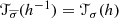 .
. -
(b)
H- equivariance: τhσ = hτσ ; that is, for any g, h ∈ H one has
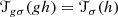 . In particular, for fixed σ0 ∈Spinc(M) the coefficients
 , or, for fixed h0 ∈ H, the coefficients
 , determine the whole τ.
-
(c)
Augmentation: Let \({\mathfrak {aug}}:\mathbb {Q}[H]\to \mathbb {Q}\) be the augmentation ∑h a(h)h↦∑h a(h). Then, for any σ one has \({\mathfrak {aug}} (\tau _\sigma )=0\) . Equivalently,
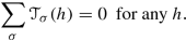
 .
. . In particular, for fixed σ0 ∈Spinc(M) the coefficients
 , or, for fixed h0 ∈ H, the coefficients
 , determine the whole τ.

4.4.14 The Fourier Transform
We wish to have a dual description of the torsion in terms of Fourier transform. First we recall the definition of the Fourier transform.
Let H be a finite abelian group and let \(\widehat {H}=\mathrm {Hom}(H, S^1)\) be its Pontryagin dual (the group of characters). If \(\chi \in \widehat {H}\) then \(\bar {\chi }\) denotes its conjugate: \(\bar {\chi }(h)=\overline {\chi (h)}\).
The Fourier transform \(\widehat {f}:\widehat {H}\to {{\mathbb C}}\) of a function \(f: H \to {{\mathbb C}}\) satisfies
Example 4.4.15
For any σ set  . Then
  .
.
Example 4.4.16
By 4.4.13 (a)–(b) for any σ, χ, h one has

4.4.6 The Reidemeister–Turaev Torsion of Graph 3-Manifolds
Let M be an oriented rational homology sphere 3-manifold associated with a connected negative definite plumbing graph Γ.
In 4.4.22 we provide a combinatorial expression in terms of Γ for the refined Reidemeister–Turaev torsion. The equivalence of this expression with the original definition of the refined torsion is proved in [78].
4.4.17 The Fourier Transform of \(Z_{h,{\mathcal I}}(t)\)
Assume that \({\mathcal I}=\{u\}\subset {\mathcal V}\) is a distinguished vertex, and for each h ∈ H we consider the reduced series \(Z_{h,{\mathcal I}}(t)\), where t is the variable corresponding to u. Set \(m_{vu}:=-(E^*_v,E^*_u)>0\). From (4.38)
This shows that the Fourier transform of the map h↦Zh,{u}(t) is
4.4.18 Character Values on Γ
Since \(\{[E^*_v]\}_v\) generate H, any character \(\chi \in \widehat {H}\) is completely characterized by the values \(\xi _v:=\chi ([E^*_v])\), \(v\in {\mathcal V}\). These are roots of unity. When we wish to identify the character χ, we put its values {ξv}v as decorations on the vertices of the graph Γ. The collection \(\{\chi ([E^*_v])\}_{v,\chi }\) is a more subtle information than the abstract group \(\widehat {H}\) itself: it shows the ‘distribution along Γ’ of the corresponding values of the characters as well. Since for any \(v\in {\mathcal V}\) one has  in H (where \(e_v=E_v^2\)), for each χ one has

Conversely, any collection of complex numbers \(\{\xi _v\}_{v\in {\mathcal V}}\), ξv ∈ S1, which satisfy (4.58) for any v, determines a character χ defined by \(\chi ([E^*_v])=\xi _v\).
Furthermore, for any \(\chi \in \widehat {H}\setminus \{1\}\), define the ‘extended support’ suppe(χ) of χ as the set of those vertices \(v\in {\mathcal V}\) for which either \(\chi ([E^*_v])\neq 1\), or v has an adjacent vertex w such that \(\chi ([E^*_w])\neq 1\).
Lemma 4.4.19
Fix a character \(\chi \in \widehat {H}\setminus \{1\}\).
-
(a)
For an arbitrary vertex u the limit \( \lim _{t\to 1}\,\widehat {Z_{\{u\}}(t)}(\chi ) \) exists and it is finite.
-
(b)
This limit is independent of u whenever u ∈suppe(χ).
Remark 4.4.20
For χ = 1, the Laurent expansion at 1 of the series \(\widehat {Z_{\{u\}}(t)}(1)\) has a non-trivial principal part, hence \( \lim _{t\to 1}\,\widehat {Z_{\{u\}}(t)}(1) \) is not finite.
4.4.21
In the sequel, the torsion  ,
,  is defined via the Fourier transform of
  in the following way.
Definition 4.4.22
-
(a)
For the trivial character
 .
. -
(b)
If \(\chi ([E^*_v])\neq 1\) for every v with κv ≠ 2, then we set

-
(c)
If χ ≠ 1, but the assumption from (b) does not hold, then the formula from (b) is regularised as follows:

for certain (any) u = uχ ∈suppe(χ).
 .
.

Theorem 4.4.23
-
(a)
 defined in
4.4.22
and the refined Reidemeister–Turaev torsion
4.4.12
coincide.
defined in
4.4.22
and the refined Reidemeister–Turaev torsion
4.4.12
coincide.
-
(b)
 defined in
4.4.22
is independent of the choice of the resolution.
defined in
4.4.22
is independent of the choice of the resolution.
 defined in
 defined in
Remark 4.4.24
-
(a)
By Fourier inversion
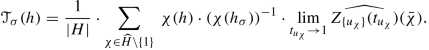
One verifies that the Properties (4.56) are valid, hence
 satisfy the duality and H-equivariance properties. Hence
 (4.59)
In particular,
 contains the same information as
  .
. -
(b)
From part (a),
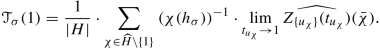
Usually, for different characters χ one needs different regularization vertices uχ. However, if ∩χ ≠ 1suppe(χ) ≠ ∅, then any u ∈ ∩χ ≠ 1suppe(χ) might serve as a common regularization vertex (with a common variable t = tu). In such a case, via \(\widehat {Z_{\{u\}}(t)}(1)=Z_{\{u\}}(t)\),

We rewrite {Zh,{u}(t)}h equivariantly as \( Z_{H,\{u\}}(t) := \sum _{h\in H}Z_{h,\{u\}}(t)h\in \mathbb {Q}[[t]][H]\), and we set \(N:=\sum _h h\in \mathbb {Q}[H]\). Then, via
 ,
,
 (4.60)
The identity (4.60) is not true in general, i.e. when ∩χ ≠ 1suppe(χ) = ∅.
The above formula already shows in this special case that the principal (pole) part of the Laurent series at t = 1 of Zh,{u}(t) is independent of h ∈ H. This statement is true in general, even without the restriction ∩χ ≠ 1suppe(χ) ≠ ∅.
-
(c)
If Γ is star-shaped then the central vertex is an element of ∩χ ≠ 1suppe(χ). Similarly, if H is cyclic, then again ∩χ ≠ 1suppe(χ) ≠ ∅.

 satisfy the duality and H-equivariance properties. Hence

 contains the same information as
  .
.

 ,
,

Example 4.4.25 (The Torsion of a Lens Space)
We fix σ = hσ σ[K] ∈Spinc(LX). Then for χ ≠ 1

Assume that \(h_\sigma =a[E^*_s]\) for some 0 ≤ a < n. Set \(\xi :=\chi ([E^*_s])\). Then,

4.4.7 Additivity Formula for the Torsion
We fix a graph Γ such that M( Γ) is a rational homology sphere. For a vertex \(v\in {\mathcal V}\) of Γ let { Γi}i be the connected components of Γ ∖ v. For any σ ∈Spinc(M( Γ)) we define its restrictions σi ∈Spinc(M( Γi)) as follows.
Choose l′ =∑w rw Ew ∈ L′ such that rv ∈ [0, 1) so that [l′] = hσ satisfies σ = σ[2l′ + K] = hσ σ[K] ∈Spinc(M( Γ)). Then we set σi = σ[Ri(2l′ + K)] = [Ri(l′)]σ[Ki] ∈Spinc(M( Γi)). (For Ri see paragraph 4.4.9.)
Theorem 4.4.26 ([12])
Set l′ =∑w rw Ew , rv ∈ [0, 1), [l′] = hσ as above. Recall also the notations from (4.52)
Then

Corollary 4.4.27
 is a rational number.
4.4.8 The Seiberg–Witten Invariant
In this section we fix a plumbed rational homology sphere 3-manifold M associated with a connected negative definite plumbing graph Γ. The Seiberg–Witten invariant of M, \({\mathfrak {sw}}\), associates to each spinc structure σ ∈Spinc(M) of M a rational number \({\mathfrak {sw}}_\sigma \). Here, based on [95], we ‘define’ it as the refined Turaev torsion modified by the Casson–Walker invariant. Based on the formulae of the previous sections, this provides \({\mathfrak {sw}}\) combinatorially from Γ.
Definition 4.4.28
We define \({\mathfrak {sw}}:\mathrm {Spin}^c(M)\to \mathbb {Q}\), \(\sigma \mapsto {\mathfrak {sw}}_\sigma \) by

Example 4.4.29
If H = 0 then Spinc(M) has only one element, and the corresponding Seiberg–Witten invariant is − λ(M) (the negative of the Casson invariant).
4.4.30 Additivity Formula for the Seiberg–Witten Invariant
The previous additivity formulae imply the following formula.
Theorem 4.4.31 ([12])
Set \(l'=\sum _wl^{\prime }_wE_w\), \(l^{\prime }_v\in [0,1)\) , as in Theorem 4.4.26 . Let σ ∈Spinc(M( Γ)) be defined as [l′]σ[K] = σ[K + 2l′], and take also its restrictions σi := [Ri(l′)]σ[Ki] = σ[Ri(K + 2l′)] too. Set hσ = [l′]. Then one has the following identities:
and

Proof
Combine Theorems 4.4.10 and 4.4.26 and use pc(S(td)) = pc(S(t)). □
This additivity formula should be compared with its ‘analytic counterpart’, namely with Okuma’s additivity formula 4.3.30.
4.4.9 The Seiberg–Witten Invariant and the Series Z(t)
We prove two key formulae for the Seiberg–Witten invariant of a rational homology sphere link. One of them identifies it with a weighted Euler characteristic of (shifted) weighted cubes in a large rectangle of \(L\otimes \mathbb R\), the other one with the constant term of the counting function of the coefficients of Z(t). The proofs are based on additivity formulae of the compared invariants.
The similarities with the analytic counterpart (the series P(t) and the equivariant genera) are emphasized.
4.4.32
In the next discussion we will use the weighted cubes, see also 4.6.3. Let us fix an element h of H and write \(L^{\prime }_h=\{l'\in L'\,:\, [l']=h\}\). Recall that the set of ‘combinatorial’ q–cubes (associated with h) consists of pairs \((l',I)\in L^{\prime }_h\times {\mathcal P}({\mathcal V})\), |I| = q (\(q\in \mathbb Z_{\geq 0}\)). (l′, I) will be identified with the vertices \(\{l'+\sum _{v\in I'}E_v\}_{I'\subset I}\) of an ‘Euclidean’ cube in \(L\otimes \mathbb R\). One defines the weight function \(w: L' \to \mathbb {Q}, \ w(l' ):=\chi (l')\), and also the a weight of the q–cubes
Assume that a set \(A\subset L\otimes \mathbb R\) has the following property: if an Euclidean cube (as above) is in A then any face of any dimension of that cube is in A. For such a set A one defines the ‘weighted Euler characteristic’
Such a set A might appear as follows. For the fixed class h ∈ L′∕L one takes two representatives \(l^{\prime }_1, \, l^{\prime }_2 \in L^{\prime }_h\) with \(l^{\prime }_2\leq l^{\prime }_1\). Then \(R_h=R_h(l^{\prime }_2,l^{\prime }_1)\) consists of the union of all combinatorial cubes (l′, I), of any dimension, such that [l′] = h and any vertex \(l'+\sum _{v\in I'}E_v\) of (l′, I) satisfies \(l^{\prime }_2\leq l'+\sum _{v\in I'}E_v \leq l^{\prime }_1\). Accordingly to the above identification, \(R_h(l^{\prime }_1,l^{\prime }_2)\) will also denote the real rectangle \(\{x\in L\otimes \mathbb R\,:\, l^{\prime }_2\leq x\leq l^{\prime }_1\}\), or the union of all Euclidean cubes (with all vertices having class [h]) in this real rectangle.
Remark 4.4.33
For a fixed h ∈ H, we can consider two types of rectangles and weighted q–cubes, depending on the geometric situation. First, in the context of lattice cohomology (see e.g. 4.6.3, and in its preparation 4.5.2) we take integral lattice points and rectangles R(l2, l1) and cubes with vertices in the lattice L, but we twist the weight function: we take χk (which generates wk) with \(k=K+2l^{\prime }_h\), for some representative \(l^{\prime }_h\) of h.
Second, when we wish to relate the cubes with the coefficients of Z(t) (as in the previous paragraph), we take shifted rectangles \(R_h:=R_h(l_2^{\prime },l^{\prime }_1)\) (\([l_j^{\prime }]=h\)) with cubes (l′, I) of type [l′] = h in them, together with the usual untwisted Riemann–Roch-function χ = χK.
The two approaches can be compared easily (see also 4.6.3). Indeed, if \(k=K+2l^{\prime }_h\), \([l^{\prime }_h]=h\), then for l ∈ L we have \(\chi (l+l^{\prime }_h)=\chi _k(l)+\chi (l^{\prime }_h)\). In particular, with the notation \(l^{\prime }_j=l_j+l^{\prime }_h\) (lj ∈ L), we have \(R_h(l^{\prime }_2,l^{\prime }_1)=l^{\prime }_h+R(l_2,l_1)\) as rectangles, and
4.4.34
Via the two incarnations of the weighted cubes (cf. 4.4.33) the next result is the ‘pair’ of Lemma 4.5.8.
Lemma 4.4.35
Fix a class h and take a representative \(l^{\prime }_0\) of h in \(-K+{\mathcal S}'\).
-
(a)
For any l′∈ L′, [l′] = h, \(l'>l^{\prime }_0\) , there exists an Ev in the support of \(l'-l^{\prime }_0\) such that w(l′− Ev) ≤ w(l′).
-
(b)
There exists a computation sequence {ℓi}i≥0 , ℓi ∈ L, with ℓ0 = 0, and ℓi+1 = ℓi + Ev(i) for some \(v(i)\in {\mathcal V}\) when i ≥ 0, satisfying:
-
(i)
The coefficients of ℓi tend to infinity, that is \(\lim _{i\to \infty } (\ell _i,-E_v^*)=\infty \) for all v.
-
(ii)
For any i ≥ 0 one has \(w(l^{\prime }_0+\ell _i)\leq w(l^{\prime }_0+\ell _{i+1})\).
-
(i)
-
(c)
For any l′ < 0, with [l′] = h, there exists Ev ∈|l′| such that w(l′ + Ev) ≤ w(l′).
-
(d)
For any representatives \(l^{\prime }_1,\, l^{\prime }_2\) of h, such that \(l^{\prime }_1\geq l^{\prime }_0>0\geq l^{\prime }_2\), \(Eu_{\chi }(R_{h}(l^{\prime }_2,l^{\prime }_1))\) is independent of the choice of \(l^{\prime }_1\) and \( l^{\prime }_2\) . In particular, with such choices, \(h\mapsto Eu_{\chi }(R_{h}(l^{\prime }_2,l^{\prime }_1))\) is a numerical invariant of h ∈ H = L′∕L.
Definition 4.4.36
The invariant provided by 4.4.35(d) will be denoted by \(\overline {\mathfrak {s}}_{h}\).
4.4.37
Let \(Z(\mathbf {t})=\sum _{l'\in L'}\mathfrak {z}(l'){\mathbf {t}}^{l'}\) be the combinatorial series defined in Sect. 4.3.3. Since Z is supported on \({\mathcal S}'\), the next sum in (4.62) is finite by 4.2.13.
Theorem 4.4.38
Fix h ∈ H. For any \(l'\in -K+{\mathcal S}'\) with [l′] = h, the expression
depends only on the class h of l′, and, in fact, it equals \(\overline {\mathfrak {s}}_{h}\) defined in 4.4.36.
Theorem 4.4.39 ([73])
For any Γ and [K + 2l′] ∈Char one has \({\mathfrak {sw}}_{\sigma [K+2l']}(M(\Gamma )) =\overline {\mathfrak {s}}_{[l']}+(K^2+|{\mathcal V}|)/8,\) or,
The proof is based on the ‘additivity formula’ 4.4.31 and a similar formula valid for \(\overline {\mathfrak {s}}_{h}\).
Therefore, Theorem 4.4.38 reads as follows.
Theorem 4.4.40
Assume that \(l'\in -K+{\mathcal S}'\) and Let \(Z(\mathbf {t})=\sum _{l'\in L'}\mathfrak {z}(l'){\mathbf {t}}^{l'}\) be the combinatorial series defined in Sect. 4.3.3 . Then
If we write l′ = rh + l (where h = [l′] and l ∈ L), then (4.64) transforms into
In particular, in the chamber \(l'=l+r_h\in -K+{\mathcal S}'\) , the sum from the left hand side of the above identities is a multivariable quadratic function in l with constant term \({\mathfrak {sw}}_{\sigma [K+2r_h]}-((K+2r_h)^2+|{\mathcal V}|)/8\).
These formulae should be compared with those from (4.36) valid for the coefficients of the series P. The fact that in (4.36) (associated with the series P) the constant terms are the equivariant geometric genera, is rather natural. However, the fact that the constant terms in the above Theorem 4.4.40 (associated with Z, a rather ‘simple’ series) is the Seiberg–Witten invariant, is rather surprising. Nevertheless, the above identity provides a very natural, direct and conceptual explanation, how the Seiberg–Witten invariant might appear in the theory of singularity links.
Example 4.4.41
If Γ is numerically Gorenstein and h = 0 then (4.65) reads as
4.4.10 The Seiberg–Witten Invariant Conjecture/Coincidence
In this section we treat a set of potential identities connecting the analytic invariants with the topological ones, namely, the equivariant geometric genera with the Seiberg–Witten invariants of the link. Whenever these identities are valid they provide a topological description of the equivariant geometric genera. The identities are generalizations of the expectation of the Casson Invariant Conjecture to the case of singularities with rational homology sphere links.
Superisolated singularities in general do not satisfy SWIC, their case will be discussed in subsection 4.4.11.
4.4.42 Seiberg–Witten Invariant Conjecture/Coincidence (SWIC) [ 73, 75, 78 ]
In this section we assume that the link of (X, o) is a rational homology sphere, and we fix a resolution \(\widetilde {X}\to X\), and we keep all the notations associated with it. We say that (X, o) satisfies SWIC(rh) for a certain h ∈ H if the following identity holds
We say that (X, o) satisfies the equivariant SWIC if (4.67) holds for every h ∈ H.
We say that (X, o) satisfies the SWIC if it satisfies SWIC(0), that is, if
The identity SWIC was formulated as a conjecture in [78] (while the equivariant case in [71]): the expectation was that it holds for any \(\mathbb {Q}\)-Gorenstein singularity. Although the conjecture can be verified for several subfamilies of singularities, since [61] we know that it is not true for the large class of \(\mathbb {Q}\)-Gorenstein singularities (see also 4.4.11 for the treatment of superisolated singularities, a family which produces several counterexamples). But even in the case of families when it fails, it still indicates interesting ‘virtual’ properties (e.g., in the superisolated case it has lead to the Semigroup Distribution Property). The limits of the validity of the SWIC are not clarified at this moment. Having in mind the existence of cases when the identities do not hold, one might say that its name as SWI ‘Conjecture’ is not totally justified, although this was its name in the literature. Hence, the reader might read the abbreviation SWIC as SWI ‘Coincidence’ too.
Example 4.4.43
Assume that (X, o) is Gorenstein and it admits a smoothing with smooth nearby (Milnor) fiber F. Then the signature satisfies \(\sigma (F)+8p_g+K^2+|{\mathcal V}|=0\), hence the SWIC (for h = 0) reads as
In this case, usually, σ(F)∕8 is not an integer, see the germ An.
Example 4.4.44
Assume that (X, o) is a complete intersection with integral homology sphere link. Then  , hence the SWIC reduces to the CIC (see 4.4.2):
Example 4.4.45
The identity P(t) = Z(t) (that is, the topological description via Z of the Poincaré series associated with the divisorial filtration) implies the equivariant SWIC. In particular, the identity P0(t) = Z0(t) implies SWIC. Indeed, for any \(l'\in -K+{\mathcal S}'\) with l′ = l + rh (l ∈ L), from (4.36) one has
On the other hand, from (4.65),
For \(l'\in -K+{\mathcal S}'\) and l′ = l + rh, we can regard the evaluation at l = 0 of the counting function \(\sum _{[\tilde {l}']=[l'],\ \tilde {l}'\not \geq l'}\mathrm {coeff}(\tilde {l}') \) as an operator. It associates with any multivariable series its ‘multivariable periodic constant’, cf. [45, 46]. In this sense, the above identities say that the periodic constant of Ph is \(h^1({\mathcal {O}}(-r_h))\), while of Zh is \({\mathfrak {sw}}_{[K+2r_h]}-((K+2r_h)^2+|{\mathcal V}|)/8\).
Hence, if Ph(t) = Zh(t) then the SWIC(rh) automatically holds as well.
In fact, in order to have the SWIC(rh) we need the validity of the above identities for a certain \(l'\in -K+{\mathcal S}'\) ([l′] = h) only. Indeed, if a certain \(l^{\prime }_0\in -K+{\mathcal S}'\), \([l^{\prime }_0]=h\), has the property that Ph(t) − Zh(t) is supported on \(\{\tilde {l}'\,:\, \tilde {l}'\geq l^{\prime }_0\}\), then by the above identities applied for this \(l^{\prime }_0\) we obtain SWIC(rh). In such a case, again by the identities (4.70)–(4.71), even if Ph(t) ≠ Zh(t), their counting functions \(l'\mapsto \sum _{[\tilde {l}']=[l'],\ \tilde {l}'\not \geq l'}\mathrm {coeff}(\tilde {l}') \) in the whole chamber \(l'\in -K+{\mathcal S}'\) coincide (independently of the position of \(l^{\prime }_0\) in this chamber).
For a fixed h, the identity Ph = Zh is much stronger than the SWIC(rh): examples when Ph ≠ Zh but the SWIC(rh) holds can be constructed.
4.4.46 Extension to the Other Natural Line Bundles
Recall that in 4.2.74 we proved that for any l′∈ L′ there exists a unique minimal \(s(l')\in {\mathcal S}'\) such that s(l′) − l′∈ L≥0. We wish to compare \(h^1({\mathcal {O}}(-l'))\) and \(h^1({\mathcal {O}}(-s(l')))\) via the SWIC property.
We say that l′∈ L′ satisfies the SWIC identity, denoted by SWIC(l′), if
If this holds, then it obviously provides a topological description for \(h^1(\widetilde {X},{\mathcal {O}}(-l'))\).
By 4.2.76 one has
A computation shows that the right hand side of (4.72) behaves similarly. Hence
Proposition 4.4.47
The SWIC(l′) is valid if and only if SWIC(s(l′)) is valid. In particular, SWIC(rh) is valid if and only if SWIC(sh) holds.
This shows that the validity of SWIC(rh) implies the validity of SWIC(l′) for all \(l'\in L^{\prime }_h\) with \(s(l')=s_{[l']}\). This covers exactly those cycles \(l'\in L^{\prime }_h \) with \(l'\leq s_{[l']}\) (including all cycles \(l'=\sum _v l^{\prime }_vE_v\) with \(l^{\prime }_v<1\) for any v).
This topological characterization SWIC(l′) of \(h^1({\mathcal {O}}(-l'))\) (modulo the validity of SWIC) in this ‘negative’ region \(\{l'\,:\, l'\leq s_{[l']}\}\) can be compared with the vanishing \(h^1({\mathcal {O}}(-l'))=0\) in the ‘opposite positive’ region \(\{l'\,:\, l'\in -K+{\mathcal S}'\}\).
It is natural to ask the following question: what can one say in the case of an arbitrary l′, which sits outside of these two regions.
Proposition 4.4.48
If SWIC(rh) holds then for any \(l'\in L^{\prime }_h\)
Additionally, if Ph = Zh (or, at least their counting functions coincide), then one has the following topological characterization of \(h^1 ({\mathcal {O}}(-l'))\):
Remark 4.4.49
Assume that the equivariant SWIC is true for (X, o). Then, taking the sum of the identities SWIC(rh) from (4.67), and using  , we get the following expression for the geometric genus of the universal abelian covering (Xa, o) in terms of the graph Γ:
Example 4.4.50 (SWIC is True for Cyclic Quotients)
In this case the link is L(n, q), \(H=\mathbb Z_n\) and the spinc structures are indexed by \(\sigma =\sigma [K+2aE_s^*]\), where \(a\in \mathbb Z\) and 0 ≤ a < n. Set also \(h=a[E^*_s]\in H\). Then

Since λ∕n = s(q, n)∕2, cf. 4.4.7, we also have
On the other hand, \((K+2r_h)^2+|{\mathcal V}|)/8=(K^2+|{\mathcal V}|)/8-\chi (r_h)\) can also be computed explicitly. From 4.2.60 one has \((K^2+|{\mathcal V}|)/8=(n-1)/4n-3\mathbf {s}(q,n)/2\).
Furthermore, from 4.2.76 we have \(h^1({\mathcal {O}}(-s_h))-h^1({\mathcal {O}}(-r_h))=\chi (s_h)-\chi (r_h)\). But \(h^1({\mathcal {O}}(-s_h))=0\) by the vanishing 4.2.71, while \(h^1({\mathcal {O}}(-r_h))=p_g(X_a,o)_{\theta (h)}=0\) (cf. 4.2.82) since the universal abelian covering (Xa, o) is smooth. Hence χ(rh) = χ(sh), and its expression is
In particular, the right hand side of SWIC(rh) is zero, and the same is true for the left hand side because of the vanishing already mentioned.
Example 4.4.51
The equivariant SWIC is true for splice quotient singularities. In particular, it is true for rational, minimally elliptic and weighted homogeneous singularities (with \(\mathbb {Q} HS^3\) link). The SWIC(0) is valid for all elliptic singularities and suspensions {zn + f(x, y) = 0}, where f is irreducible (and with \(\mathbb {Q} HS^3\) link).
4.4.11 SWIC and Superisolated Singularities
We assume that (X, o) is a superisolated singularity associated with the irreducible projective rational cuspidal curve C of degree d.
Though in many cases (e.g. for weighted homogeneous singularities) we discuss the SWIC together with equivariant SWIC, this is not the case for the superisolated germs. The main obstruction is that in the superisolated case (though pg(X, o) and \(P_{0,\{v_+\}}(t)\) are extremely simple), usually we have very little information about the analytic properties of the universal abelian covering, e.g. about its geometric genus pg(Xa, o) (see e.g. [111]). Therefore, in this subsection we focus merely on the SWIC (for h = 0).
It turns out that for a superisolated singularity the SWIC is valid if and only if N(1) = 0, a property which is not always true, cf. subsection 4.3.6. Let us list first the involved invariants.
4.4.52
From Example 4.4.11 we have \(K^2+|{\mathcal V}|=-d(d-2)^2+1\) and  (μ = 2δ). Moreover, the divisorial filtration associated with \({\mathcal I}=\{C\}=\{v_+\}\) agrees with the filtration associated with weights (1, 1, 1), hence \(P_{0,{\mathcal I}}(t)=(1-t^d)/(1-t)^3\). Since in the good resolution Γ ∖ v+ supports only smooth germs, by 4.3.30
\(p_g(X,o)=\mathrm {pc}(P_{0,{\mathcal I}}(t))\), which is d(d − 1)(d − 2)∕6.
(μ = 2δ). Moreover, the divisorial filtration associated with \({\mathcal I}=\{C\}=\{v_+\}\) agrees with the filtration associated with weights (1, 1, 1), hence \(P_{0,{\mathcal I}}(t)=(1-t^d)/(1-t)^3\). Since in the good resolution Γ ∖ v+ supports only smooth germs, by 4.3.30
\(p_g(X,o)=\mathrm {pc}(P_{0,{\mathcal I}}(t))\), which is d(d − 1)(d − 2)∕6.
The definition of \(Z_{\mathcal I}(t)\) compared with A’Campo formula [1] gives

Since H is generated by \([E^*_+]\), the vertex v+ (corresponding to C) is a regularization vertex for any character. Therefore, from 4.4.24

Following 4.3.6 we also consider

Then

If we write  as in 4.3.6, then the limit can be computed in terms of d and
  . The computation provides
Proposition 4.4.53
This combined with (4.45) gives (with \(Q(t)=\sum _{j=0}^{\mu -2}\alpha _jt^j\) )
Corollary 4.4.54
-
(a)
SWIC for h = 0 is equivalent to N(1) = 0.
-
(b)
The Conjecture 4.3.22 (which predicts that N(1) ≤ 0 for any superisolated singularity) is equivalent to \({\mathfrak {sw}}_{\sigma [K]}-\frac {K^2+|{\mathcal V}|}{8}\leq p_g\).
Corollary 4.4.54 has the following consequences (for some of the arguments see the paragraphs after 4.3.21): via the ‘Semigroup Distribution Property’ 4.2.33, the SWIC (for h = 0) is valid whenever ν = 1. In fact, in this case not only N(1) = 0, but even N(t) ≡ 0, i.e. \(Z_{0,{\mathcal I}}(t)\equiv P_{0,{\mathcal I}}(t)\).
If ν = 2 then the coefficients of N(t) are non-positive, however, it can happen that N(t) ≠ 0, see. e.g. several examples in [61]. Hence, if ν = 2 and N(t) ≠ 0 then the SWIC fails and \({\mathfrak {sw}}_{\sigma [K]}-\frac {K^2+|{\mathcal V}|}{8}< p_g\). (The difference will be interpreted in terms of lattice cohomology in 4.9.2.)
Remark 4.4.55
Though till now we tried to convince the reader that the SWIC, for certain analytic types, is a ‘natural’ reality, the superisolated case suggests the opposite. Indeed, for such germs, pg depends only on d, but the topological side depends in a subtle way on the local singularity types of C (see above the formulae of λ and  ). Having in mind this subtle sensitivity to the local singularity data of C, the validity of SWIC (when it holds) is a true marvel.
Example 4.4.56
Let us analyse a particular case with more details. Assume d = 5, ν = 2, and the two singularities have multiplicity sequence [3] and [23]. The graph Γ is presented below, and N(t) = −2t, hence SWIC fails: pg = 10, while − λ = 21∕2 and  , hence \({\mathfrak {sw}}_{\sigma [K]}-(K^2+|{\mathcal V}|)/8=8\).

In fact, we can consider two analytic structures supported on this topological type (given by the graph). They are rather different, though both are very natural. The first is a superisolated hypersurface singularity, as analysed above. On the other hand, this topological type supports also a splice quotient singularity which satisfies SWIC, hence it has pg = 8.
4.5 Weighted Cubes and the Spaces Sk,n
4.5.1 Weighted Cubes and Generalized Computation Sequences
To any good resolution graph Γ and characteristic element k ∈Char, we consider the weight function \(\chi _k:L\to \mathbb Z\), and a natural cubical decomposition of \(\mathbb R^s\) associated with the embedding \(L\simeq \mathbb Z^s\hookrightarrow \mathbb Z^s\otimes \mathbb R=\mathbb R^s\), where \(s=|\mathcal {V}|\) and the identification \(L\simeq \mathbb Z^s\) is given by the base vectors \(\{E_v\}_{v\in \mathcal {V}}\). Then, for each n ≥minl ∈ L{χk(l)}, we define the topological space Sk,n, as the union of all cubes, which have all vertices of weight ≤ n. We show that the homotopy type of the tower {Sk,n}n depends only on the 3-manifold M( Γ) and on the spinc structure associated with k. The tower {Sk,n}n carries an extremely deep information about M( Γ); the final goal is to determine their homotopy types. Via the spaces {Sk,n}n this section prepares the theory of graded roots and lattice cohomology.
4.5.1 Cubes in \(L\otimes \mathbb R\) and the Spaces {Sk,n}n [ 72 ]
Fix a connected plumbing graph Γ with negative definite intersection form, and we assume that the plumbed 3-manifold M( Γ) is a rational homology sphere.
We use the standard notations for the lattice L, which has the distinguished base elements \(\{E_v\}_{v\in {\mathcal V}}\). Using this basis, one identifies L with \(\mathbb Z^s\) with its fixed standard basis, still denoted by \(\{E_v\}_{v\in {\mathcal V}}\).
\(\mathbb Z^s\otimes \mathbb R\simeq \mathbb R^s\) has a natural decomposition into cubes given by the inclusion \(\mathbb Z^s\hookrightarrow \mathbb R^s\). The zero-dimensional cubes are exactly the lattice points \(\mathbb Z^s\). Any \(l\in \mathbb Z^s\) and subset \(I\subset {\mathcal V}\) of cardinality q defines a q-dimensional cube □q = (l, I), which has its vertices in the lattice points \((l+\sum _{v\in I'}E_v)_{I'}\), where I′ runs over all subsets of I.
Next, we fix a characteristic element k ∈Char and we consider the Riemann–Roch function \(\chi _k:L\to {\mathbb Z}\), χk(l) = −(l, l + k)∕2. Here we regard χk as a weight function on the set of cubes: the weights of zero-dimensional cubes are defined by w0(l) = χk(l), while, in general, \(w_q((l,I)):=\max \{\chi _k(v)\,:\, v \ \, \mbox{is a vertex of }(l,I)\}\).
Definition 4.5.2
For every \(n\in \mathbb Z\), define \(S_n\subset \mathbb R^s\) as the union of all the cubes □q, of any dimension, with w(□q) ≤ n (with induced topology of \(\mathbb R^s\)). Clearly, Sn ≠ ∅ exactly when n ≥ mk, where \(m_k:=\min _{l\in \mathbb Z^s}\chi _k(l)\). If we wish to emphasize the k-dependence we write Sk,n.
One has the natural inclusions \(S_{m_k}\subset \ldots \subset S_n\subset S_{n+1}\subset \ldots \). It turns out that the topology of the spaces \(\{S_n\}_{n\geq m_k}\) might be rather interesting. The tower has a finiteness property: only finitely many Sn have nontrivial topology (are non-contractible), but an Sn with n ‘small’ might have rather complicated homology groups. In general it is rather hard to solve the corresponding Diophantine equations and to analyse the adjacent positions of the solutions (in order to get the cubes which build up the topological space Sn). However, this combinatorial/artihmetical structure can be extremely rich covering a big amount of deep information.
Example 4.5.3 ([72])
Consider the following graph:

A computation shows that χ ≥−1. S−1 consists of two contractible connected components. The space S0 has three connected components, two of them contractible, and the third has the homotopy type of the circle. The spaces Sn for n ≥ 1 are contractible.
4.5.4
Assume that k and k′ determine the same Spinc–structure of M( Γ), cf. 4.2.94, hence k′ = k + 2l for some l ∈ L. Then \(\chi _{k'}(x-l)=\chi _k(x)-\chi _k(l)\) for any x ∈ L. This means that the transformation x↦x′ := x − l realizes an identification of the ‘Sn-spaces’ associated with k and k′: \( S_{k, n}=S_{k', n-\chi _k(l)}\). Hence, fixing a representative k from each class [k] ∈Spinc(M( Γ)) we can speak about the tower of spaces {Sk,n}n, indexed by [k] ∈Spinc(M( Γ)).
Proposition 4.5.5 ([72])
The tower of spaces {Sk,n}n , indexed by [k] ∈Spinc(M( Γ)), up to homotopy equivalence, depends only on M = M( Γ), it is independent of the choice of the negative definite plumbing graph Γ, which provides M.
Remark 4.5.6
A possible generalization of the set of weighted cubes and spaces Sn is provided via a set of compatible weight functions. Let \({\mathcal Q}_q\) denote the set of q–cubes. A set of functions \(w_q:{\mathcal Q}_q\to \mathbb Z\) (\(0\leq q\leq |\mathcal {V}|\)) is called a set of compatible weight functions if the following hold:
-
(a)
for any integer \(n\in \mathbb Z\), the set \(w_0^{-1}((-\infty ,n])\) is finite;
-
(b)
for any \(\square _q\in {\mathcal Q}_q\) and for any of its faces \(\square _{q-1}\in {\mathcal Q}_{q-1}\) one has wq(□q) ≥ wq−1(□q−1).
Then one can define Sn as \(\cup _q \{\square \in {\mathcal Q}_q\,:\, w_q(\square _q)\leq n\}\).
4.5.2 The Topology of the Spaces {Sk,n}n
In order to analyse the topology of the space Sn = Sn,k it is convenient to introduce the set of finite rectangles indexed by pairs l1, l2 ∈ L with l1 ≤ l2.
Definition 4.5.7
For any such pair l1 ≤ l2 set \(R(l_1,l_2):=\{x\in \mathbb R^s\,:\, l_1\leq x\leq l_2\}\). Define also \(R(l_1,\infty ):=\{x\in \mathbb R^s\,:\, l_1\leq x\}\).
The point in the next lemma is that χ-monotone (non-increasing) computation sequences provide strong deformation retracts for the spaces Sk,n.
Lemma 4.5.8
Fix k ∈Char and write Sn = Sk,n.
-
(I)
There exist l+ ∈ L and an increasing infinite sequence of cycles {li}i≥0 (li ∈ L) with l0 = l+ , such that
-
(a)
for any i ≥ 0 one has li+1 = li + Ev(i) for some \(v(i)\in \mathcal {V}\),
-
(b)
if li =∑v mi,v Ev , then limi→∞ mi,v = ∞ for all v,
-
(c)
χk(li+1) ≥ χk(li).
Similarly, there exists l−∈ L and an increasing infinite sequence of cycles {yi}i≥0 , satisfying y0 = l− , the analogs of (a)–(b), and (c) χk(−yi+1) ≥ χk(−yi).
-
(a)
-
(II)
Take l− and l+ as in (I). Without loss of generality we can assume that − l−≤ l+ . Then the inclusion R(−l−, ∞) ∩ Sn ⊂ Sn and R(−l−, l+) ∩ Sn ⊂ Sn are homotopy equivalences for any \(n\in \mathbb Z\).
Corollary 4.5.9
For any k ∈Char the space Sn is contractible for any n ≫ 0.
Proof
Fix l−≤ l+ as in Lemma 4.5.8 (I). Let n be so large that R(−l−, l+) ⊂ Sn. Then, by Lemma 4.5.8 (II) Sn has the same homotopy type as R(−l−, l+). □
4.5.10 Distinguished Representatives and Their Spaces Sn
As we already said in 4.5.4, if k′ = k + 2l for some l ∈ L then \( S_{k, n}=S_{k', n-\chi _k(l)}\). Hence, it is natural to choose one representative from each spinc structure. For several results the choice is irrelevant, however, certain choices have certain advantages. Our preferred choice is the distinguished representative, or distinguished characteristic element kr := K + 2sh, cf. 4.2.94, where sh ∈ L′ is the smallest representative of h in \({\mathcal S}'\), cf. 4.2.78.
A possible motivation for the choice of kr is the following. Recall that the rationality criterion for graphs is χ(l) > 0 for any l ∈ L>0, hence it is decided in the ‘first quadrant’ L≥0 of L. More generally, for arbitrary graphs, the essential properties of \(\chi :L\to \mathbb Z\) are already coded in the restriction χ|L≥0. The choice kr = K + 2sh guarantees that the essential properties of \(\chi _{k_r}:L\to \mathbb Z\) are coded again in L≥0 (or, equivalently, for a fixed h, the essential information of \(\chi _{\mathbb {Q}}|\{l'\in L'\,:\, [l']=h\}\) is coded in \(\chi _{\mathbb {Q}}|s_h+L_{\geq 0}\).
Lemma 4.5.11
Fix h ∈ H and kr = K + 2sh as above. Then the following facts hold.
-
(a)
In Lemma 4.5.8 one may take l− = 0. This means that \(R(0,\infty )\cap S_{k_r,n}\subset S_{k_r,n}\) is a homotopy equivalence for any n. In particular, by Lemma 4.5.8 , there exists l+ ≥ 0 such that \(R(0,l_+)\cap S_{k_r,n}\subset S_{k_r,n}\) is a homotopy equivalence for any n.
-
(b)
Assume that ZK ≥ 0 (e.g., as in the minimal good resolution). Then one can take l+ = ⌊ZK⌋. Hence, \(S_{k_r,n}\) has the homotopy type of \(R(0,\lfloor Z_K \rfloor )\cap S_{k_r,n}\).
-
(c)
For any x ≥ 0 one has \(\chi _{k_r}(x)\geq \chi _{K}(x)\) . Therefore, \(\min \chi _{k_r}\geq \min \chi _K\).
-
(d)
SK,n (i.e. when h = 0 and sh = 0) is connected for all n ≥ 1.
Example 4.5.12 (Characterization of Rational Graphs via the Spaces Sn [70])
Let Γ be a connected, negative definite plumbing graph whose plumbed 3-manifold is a rational homology sphere. Recall that Γ is rational if χ(l) > 0 for any l ∈ L>0. (In this case pg(X, o) = 0 for any analytic type supported on the topological type determined by Γ.) Then the following facts are equivalent:
-
(a)
Γ is rational;
-
(b)
SK,n is contractible for every \(n\geq \min \chi \);
-
(b′)
SK,n is connected for every \(n\geq \min \chi \);
-
(c)
Sk,n is contractible for all k ∈Char and \(n\geq \min \chi _k\).
Additionally, if Γ is rational and kr = K + 2sh, then \(\min \chi _{k_r}=0\).
Example 4.5.13 (Characterization of Elliptic Graphs via the Spaces SK,n [70])
Assume again that M( Γ) is a \(\mathbb {Q} HS^3\). Recall that Γ is elliptic if \(\min \chi =0\) and Γ is not rational. Then Γ is elliptic if and only if SK,n is empty for n < 0 and SK,0 is not connected.
4.5.3 ‘Bad’ Vertices, Almost Rational Graphs and Lattice Fibrations
We measure how far an arbitrary graph (tree) Γ is from being rational. Recall that decreasing all the self-intersection numbers of a tree, with all the vertices decorated by gv = 0, we obtain a rational graph. The next definition aims to identify those vertices where such a decrease is really necessary. [Such a subset of \({\mathcal V}\) was already considered in different articles like [70, 72, 74, 102], mostly under the name ‘bad vertices’. Since the definition of the ‘badness’ was not uniform here we use the notation SR for them, for several other families see [66].]
Definition 4.5.14
Let Γ be a negative definite connected tree with M( Γ) a \(\mathbb {Q} HS^3\).
A subset of vertices \(\overline {{\mathcal V}}=\{v_1,\ldots , v_\nu \}\subset {\mathcal V}\) is called SR–set, if by replacing the Euler numbers \(e_v=E_v^2\) indexed by \(v\in \overline {{\mathcal V}}\) by some more negative integers \(e^{\prime }_v\leq e_v\) we get a rational graph. A graph is called AR-graph (‘almost rational graph’) if it admits an SR–set of cardinality ≤ 1.
Example 4.5.15
-
(a)
A possible SR–set can be chosen in many different ways, it is not determined uniquely even if it is minimal with this property.
-
(b)
Usually we allow non-minimal SR–sets as well.
-
(c)
Any rational graph is AR; for rational graphs the empty set is an SR–set. The class of AR graphs is closed while taking subgraphs or/and decreasing the Euler numbers.
-
(d)
The set of nodes is an SR–set. Hence any star-shaped graph (with g = 0) is AR with \(\overline {{\mathcal V}}=\{v_0\}\).
-
(e)
Any elliptic graph with \(H_1(L_X,\mathbb {Q})=0\) is AR.
-
(f)
Consider the graph Γ of \(S^3_{-d}(K)\) (for d > 0 and K ⊂ S3 algebraic knot). Then Γ is AR: if we modify the − 1 decoration of v1 into − 2, we get a sandwiched (hence rational) graph.
-
(g)
Let \(\{K_i\}_{i=1}^\nu \) be algebraic knots and set K = #i Ki. For d > 0 the negative definite graph Γ of \(S^3_{-d}(K)\) is given in 4.2.32. Then the smallest SR–set consists of the set of (−1)-vertices (their number is ν).
4.5.16 Lattice Fibrations: Universal Cycles in the Fibers
Let us give some intuition for the next construction.
If Γ is rational, then 0 is a \(\chi _{k_r}\)–minimal lattice point, and \(0\hookrightarrow S_{k_r,n}\) (n ≥ 0) admits a strong deformation retraction: there is a \(\chi _{k_r}\)–non-increasing (combinatorial) flow contracting any \(S_{k_r,n}\) (and \(L\otimes {\mathbb R}\)) to 0.
In general, let us start with the lattice L and a representative \(k=K+2l^{\prime }_h\). Then (dictated by some ‘badness properties’ of some of the vertices, indexed by \(\overline {{\mathcal V}}\)) we will write the set of vertices \({\mathcal V}\) as a disjoint union \(\overline {{\mathcal V}}\sqcup {\mathcal V}^*\), such that any sublattice of type \( \bar {l}+L({\mathcal V}^*)\) (where \(\bar {l}=\sum _{v\in \overline {{\mathcal V}}} \ell _vE_v\in L(\overline {{\mathcal V}})\)) behaves as a rational lattice, that is, it can be contracted to one of its lattice points via a χk–non-increasing flow. (In other words, ‘L, or the spaces Sn, project to \(L(\overline {{\mathcal V}})\) with contractible fibers’.) On the other hand, the χk–minimal point of \(\bar {l}+L({\mathcal V}^*)\), where \(\bar {l}+L({\mathcal V}^*)\) contracts, depends essentially on \(\bar {l}\); it is a crucial universal point \(x_{l^{\prime }_h}(\bar {l})\) of \(\bar {l}+L({\mathcal V}^*)\). The aim of different reduction theorems is to recover different invariants of the weighted lattice (L, χk) from \(\{\chi _{k}(x_{l^{\prime }_h}(\bar {l}))\}_{\bar {l}\in L(\overline {{\mathcal V}})}\).
In this subsection we define and analyse the points \(x_{l^{\prime }_h}(\bar {l})\). If \(l^{\prime }_h=s_h\) then some additional ‘positivity’ properties hold for them.
4.5.17 The Definition of the Lattice Points \(x(\bar {l})\)
Let us fix a resolution of a germ (whose link is not necessarily a rational homology sphere). Suppose we have a family of distinguished vertices \(\overline {{\mathcal V}}:=\{v_k\}_{k=1}^\nu \subseteq {\mathcal V}\) (usually chosen by a certain geometric property). Then we split the set of vertices \({\mathcal V}\) into the disjoint union \(\overline {{\mathcal V}}\sqcup {\mathcal V}^*\). Let {mv(x)}v denote the coefficients of a cycle \(x\in L\otimes \mathbb {Q}\), that is \(x=\sum _{v\in {\mathcal V}}m_v(x)E_v\).
We use the notation \(\bar {l}:=\sum _{v\in \overline {{\mathcal V}}}\ell _v E_v\in L(\overline {{\mathcal V}})\), and we fix h ∈ H and a representative \(l^{\prime }_h\in L'\) with \([l^{\prime }_h]=h\). Then the cycles \(x(\bar {l})\) are defined as follows.
Proposition 4.5.18 ([70, Lemma 7.6], [47])
For any \(\bar {l}\in L(\overline {{\mathcal V}})\) there exists a unique cycle \(x(\bar {l})\in L\) (depending on the choice of \(l^{\prime }_h\) ) satisfying the next properties:
-
(a)
\(m_{v}(x(\bar {l}))=\ell _v\) for any distinguished vertex \(v\in \overline {{\mathcal V}}\);
-
(b)
\((x(\bar {l})+l^{\prime }_h,E_v)\leq 0\) for every ‘non-distinguished vertex’ \(v\in {\mathcal V}^*\);
-
(c)
\(x(\bar {l})\) is minimal with the two previous properties (with respect to ≤).
Furthermore, the cycle \(x(\bar {l})\) automatically satisfies
If we wish to emphasize the dependence on \(l^{\prime }_h\) we write \(x_{l^{\prime }_h}({\bar l})\).
The cycles \(x(\bar {l})\) satisfy the following universal property as well.
Lemma 4.5.19
Assume that a certain x ∈ L satisfies \(m_{v}(x)= m_{v}(x(\bar {l}))\) for all \(v\in \overline {{\mathcal V}}\) , and \(x\leq x(\bar {l})\).
Then there is a generalized Laufer’s computation sequence connecting x with \(x(\bar {l})\) . The sequence \(\{z_i\}_{i=0}^t\) is constructed as follows. Set z0 = x. Assume that zi is already constructed. If for some \(v\in {\mathcal V}^*\) one has (zi + sh, Ev) > 0 then take zi+1 = zi + Ev(i) , where v(i) is such an index. If zi satisfies 4.5.18 (b), then stop and set t = i. Then this procedure stops after finite steps and zt is exactly \(x(\bar {l})\).
Along the computation sequence χk(zi+1) ≤ χk(zi) for any 0 ≤ i < t. Equality holds if \((z_i+l^{\prime }_h,E_{v(i)})=1\).
In the case of an SR–set we have the following statement.
Proposition 4.5.20
Let \(\overline {{\mathcal V}}\) be an SR–set. Choose \(l^{\prime }_h\) and set \(k=K+2l^{\prime }_h\) . Then \(\bar {l}+L({\mathcal V}^*)=\{x\in L\,:\, m_{v}(x)= m_{v}(x(\bar {l})) \ \mathit{\mbox{for all }}v\in \overline {{\mathcal V}}\}\) contracts to \(x(\bar {l})\) such that along the contraction χk is non-increasing. In particular, \(\chi _{k}(x)\geq \chi _{k_r}(x(\bar {l}))\) for any \(x\in \bar {l}+L({\mathcal V}^*)\).
4.5.4 Concatenated Computation Sequences of AR Graphs [70]
Assume that Γ is an AR resolution graph, let {v0} be an SR–set. In particular M( Γ) is a rational homology sphere.
Theorem 4.5.21
If Γ is AR, then for any k ∈Char and \(n\geq m_k=\min \chi _k\) any connected component of Sk,n is contractible.
Note that the statement is independent of the choice of k in its class, cf. 4.5.10. In the sequel we will choose the distinguished representative kr, and we write Sn for \(S_{k_r,n}\). We also write \(\mathcal {V}=\overline {{\mathcal V}}\sqcup \mathcal {V}^*\), where \(\overline {{\mathcal V}}=\{v_0\}\). For each \(\ell \in \mathbb Z\) we consider the cycles \(\bar {l}:=\ell E_{v_0}\in L({\overline {{\mathcal V}}})\) and \(x(\bar {l})\in L \) from 4.5.16. We abridge \(x(\ell E_{v_0})\) as x(ℓ).
In order to prove the theorem we construct an increasing path γ = {li}i≥0 in L (with ℓi+1 = ℓi + Ev(i) for all i), which determines the 1-chain Cγ := ∪i≥0[li, li+1] of 1-cubes in \(L\otimes \mathbb R\) (without any loop), such that Cγ ∩ Sn↪Sn is a homotopy equivalence. The construction and the statement of the theorem constitute the prototype of the more general Reduction Theorem 4.8.2 and also this was the original intuitive motivation and starting point in the definition of the graded roots, cf. 4.7 and 4.7.2.
The construction start as follows. By Lemma 4.5.11 (a) the inclusion R(0, ∞) ∩ Sn ⊂ Sn admits a strong deformation retract. Hence we can restrict ourself to the intersection with the first quadrant. The path γ = {li}i≥0 is defined as a series of concatenated computation sequences. It contains, as intermediate terms, all the universal cycles {x(ℓ)}ℓ≥0 in an increasing order. The first term is l0 = x(0) = 0. The part of the sequence starting from x(ℓ) and ending with x(ℓ + 1) starts with x(ℓ) and the next term is \(x(\ell )+E_{v_0}\). Then, the continuation is generalized Laufer-type computation sequence connecting \(x(\ell )+E_{v_0}\) with x(ℓ + 1). Indeed, the multiplicity of E0 in both \(x(\ell )+E_{v_0}\) and x(ℓ + 1) is ℓ + 1, and by (4.75) \(x(\ell +1)\geq x(\ell )+E_{v_0}\). Hence Lemma 4.5.19 gives a computation sequence \(\gamma ^{(\ell +1)}=\{l_i^{(\ell +1)}\}_i\), which connects them. Then we proceed inductively.
Define \(\tau (\ell ):=\chi _{k_r}(x(\ell ))\). Let o be the order of \(E^*_{v_0}\) in L′∕L and \(p=m_{v_0}(oE^*_{v_0})\).
Lemma 4.5.22
-
(a)
The path {li}i is increasing: li+1 = li + Ev(i).
-
(b)
For any Ev -coefficient one has limℓ→∞ mv(x(ℓ)) = ∞ (where \(v\in \mathcal {V}\) ).
-
(c)
(Quasiperiodicity) \(x(\ell +tp)=x(\ell )+toE^*_{v_0}\).
-
(d)
\(\chi _{k_r}\) along each part (subsequence) γ (ℓ) is constant.
-
(e)
\(\tau (\ell +1)=\tau (\ell )+1-(x(\ell )+s_h,E_{v_0})\).
-
(f)
There exists ℓ0 such that τ(ℓ + 1) ≥ τ(ℓ) for ℓ ≥ ℓ0.
Theorem 4.5.23
Consider the 1-chain Cγ := ∪i≥0[li, li+1] in \(L\otimes \mathbb R\) as above. Then for any n the inclusion Cγ ∩ Sn ⊂ Sn is a homotopy equivalence. In particular, since each connected component of Cγ ∩ Sn is contractible, Theorem 4.5.21 follows.
Remark 4.5.24
In general, it is not easy to find the cycles x(ℓ). Fortunately, in several applications (see e.g. 4.7.3) one does not need all the coefficients of these cycles, only the values \(\tau (\ell )=\chi _{k_r}(x(\ell ))\). In most of the cases they are computed inductively using 4.5.22 (e), hence basically one needs only to know \((x(\ell ),E_{v_0})\) for any ℓ.
Example 4.5.25
For the determination of the universal cycles {x(ℓ)}ℓ and the corresponding τ-function in the case of star-shaped graphs and surgery manifolds see 4.7.22, 4.7.4 and Sect. 4.9.
4.6 Lattice Cohomology
We provide two equivalent definitions for the lattice cohomology \(\{\mathbb H^q\}_{q\geq 0}\) associated with a free \(\mathbb Z\)-module endowed with a fixed basis and with a set of ‘compatible weight functions’. The first definition is based on the construction of a cochain complex. The second one involves the spaces {Sn}n introduced in 4.5.2. Once Γ is fixed, any characteristic element k ∈Char determines a set of weights (via the RR expression χk), hence the lattice cohomology \(\mathbb H^*(\Gamma ,k)\). It turns out that they depend only on M( Γ) and [k] ∈Spinc(M( Γ)). In 4.6.3 we show that the Euler characteristic of \(\mathbb H^*(\Gamma ,k)\) is the normalized Seiberg–Witten invariant of M( Γ).
For more details see e.g. [71,72,73].
4.6.1 The Lattice Cohomology Associated with a System of Weights
We consider a free \(\mathbb Z\)-module, with a fixed basis \(\{E_v\}_{v\in \mathcal {V}}\), denoted by \(\mathbb Z^s\). It is also convenient to fix a total ordering of the index set \(\mathcal {V}\), which in the sequel will be denoted by {1, …, s}. Our goal is to define a graded \(\mathbb Z[U]\)-module associated with the pair \((\mathbb Z^s, \{E_v\}_v)\) and a set of weights. First we set some notations regarding \(\mathbb Z[U]\)-modules.
4.6.1 \({\mathbb Z[U]}\)-Modules
Consider the graded \(\mathbb Z[U]\)-module \({\mathcal T}:=\mathbb Z[U,U^{-1}]\), and (following [102]) denote by \({\mathcal T}_0^+\) its quotient by the submodule \(U\cdot \mathbb Z[U]\). This has a grading in such a way that deg(U−d) = 2d (d ≥ 0). Similarly, for any n ≥ 1, the quotient of \(U^{-(n-1)}\cdot \mathbb Z[U]\) by \(U\cdot \mathbb Z[U]\) (with the same grading) defines the graded module \({\mathcal T}_0(n)\). Hence, \({\mathcal T}_0(n)\), as a \(\mathbb Z\)-module, is freely generated by 1, U−1, …, U−(n−1), and has finite \(\mathbb Z\)-rank n.
More generally, for any graded \(\mathbb Z[U]\)-module P with d-homogeneous elements Pd, and for any \(r\in \mathbb {Q}\), we denote by P[r] the same module graded (by \(\mathbb {Q}\)) in such a way that P[r]d+r = Pd. Then set \({\mathcal T}^+_r:={\mathcal T}^+_0[r]\) and \({\mathcal T}_r(n):={\mathcal T}_0(n)[r]\). Hence, for \(m\in \mathbb Z\), \({\mathcal T}_{2m}^+=\mathbb Z\langle U^{-m}, U^{-m-1},\ldots \rangle \) as a \(\mathbb Z\)-module.
4.6.2 The Cochain Complex
\(\mathbb Z^s\otimes \mathbb R\) has a natural cellular decomposition into cubes (see also 4.5.1). The set of zero-dimensional cubes is provided by the lattice points \(\mathbb Z^s\). Any \(l\in \mathbb Z^s\) and subset \(I\subset \mathcal {V}\) of cardinality q defines a q-dimensional cube, which has its vertices in the lattice points \((l+\sum _{v\in I'}E_v)_{I'}\), where I′ runs over all subsets of I. On each such cube we fix an orientation. This can be determined, e.g., by the order \((E_{v_1},\ldots , E_{v_q})\), where v1 < ⋯ < vq, of the involved base elements {Ev}v ∈ I. The set of oriented q-dimensional cubes defined in this way is denoted by \({\mathcal Q}_q\) (0 ≤ q ≤ s).
Let \({\mathcal C}_q\) be the free \(\mathbb Z\)-module generated by oriented cubes \(\square _q\in {\mathcal Q}_q\). Clearly, for each \(\square _q\in {\mathcal Q}_q\), the oriented boundary ∂□q (of ‘classical’ cubical homology) has the form \(\sum _k\varepsilon _k \, \square _{q-1}^k\) for some εk ∈{−1, +1}. These are the faces of □q. It is clear that ∂ ∘ ∂ = 0. But, obviously, the homology of the chain complex \(({\mathcal C}_*,\partial )\) (or, of the dual cochain complex \(({\mathrm {Hom}}_{\mathbb Z}({\mathcal C}_*,\mathbb Z),\delta )\)) is not very interesting: it is the (co)homology of \(\mathbb R^s\). A more interesting (co)homology can be constructed as follows. For this, we consider a set of compatible weight functions {wq}q as in 4.5.6. In the sequel sometimes we will omit the index q of wq.
4.6.3
In the presence of any fixed set of compatible weight functions {wq}q we define \({\mathcal F}^q\) as the set of morphisms \({\mathrm {Hom}}_{\mathbb Z}({\mathcal C}_q,{\mathcal T}^+_0)\) with finite support on \({\mathcal Q}_q\).
Notice that \({\mathcal F}^q\) is a \(\mathbb Z[U]\)-module by (p ∗ ϕ)(□q) := p(ϕ(□q)) (\(p\in \mathbb Z[U]\)). Moreover, \({\mathcal F}^q\) has a \(\mathbb Z\)-grading: \(\phi \in {\mathcal F}^q\) is homogeneous of degree \(\mathrm {deg}(\phi )=d\in \mathbb Z\) if for each \(\square _q\in {\mathcal Q}_q\) with ϕ(□q) ≠ 0, ϕ(□q) is a homogeneous element of \({\mathcal T}^+_0\) of degree d − 2 ⋅ w(□q). (In fact, the grading is \(2\mathbb Z\)-valued; hence, the reader interested only in the present construction may divide all the degrees by two. Nevertheless, we prefer to keep the present form in our presentation because of its resonance with the Heegaard Floer homology of the link.)
Next, we define \(\delta _w:{\mathcal F}^q\to {\mathcal F}^{q+1}\). For this, fix \(\phi \in {\mathcal F}^q\) and we show how δw ϕ acts on a cube \(\square _{q+1}\in {\mathcal Q}_{q+1}\). First write \(\partial \square _{q+1}=\sum _k\varepsilon _k \square ^k_q\), then set
Lemma 4.6.4
δw ∘ δw = 0, i.e. \(({\mathcal F}^*,\delta _w)\) is a cochain complex.
4.6.5
In fact, \(({\mathcal F}^*,\delta _w)\) has a natural augmentation too. Indeed, set \(m_w:=\min _{l\in \mathbb Z^s}w_0(l)\) and choose \(l_w\in \mathbb Z^s\) such that w0(lw) = mw. Then one defines the \(\mathbb Z[U]\)-linear map
such that \(\epsilon _w (U^{-m_w-s})(l)\) is the class of \(U^{-m_w+w_0(l)-s}\) in \({\mathcal T}^+_0\) for any l ∈ L and s ≥ 0.
Lemma 4.6.6
𝜖w is injective, and δw ∘ 𝜖w = 0.
One verifies that both 𝜖w and δw are morphisms of \(\mathbb Z[U]\)-modules and are homogeneous of degree zero.
Definition 4.6.7
The homology of the cochain complex \(({\mathcal F}^*,\delta _w)\) is called the lattice cohomology of the pair \((\mathbb R^s,w)\), and it is denoted by \(\mathbb H^*(\mathbb R^s,w)\). The homology of the augmented cochain complex

is called the reduced lattice cohomology of the pair \((\mathbb R^s,w)\), and it is denoted by \(\mathbb H_{red}^*(\mathbb R^s,w)\).
If the pair \((\mathbb R^s,w)\) is clear from the context, we omit it from the notation.
For any q ≥ 0 fixed, the \(\mathbb Z\)-grading of \({\mathcal F}^q\) induces a \(\mathbb Z\)-grading on \(\mathbb H^q\) and \(\mathbb H^q_{red}\); the homogeneous part of degree d is denoted by \(\mathbb H^q_d\), or \(\mathbb H^q_{red,d}\). Moreover, both \(\mathbb H^q\) and \(\mathbb H_{red}^q\) admit an induced graded \(\mathbb Z[U]\)-module structure and \(\mathbb H^q=\mathbb H^q_{red}\) for q > 0.
It is easy to see that \(\mathbb H^*(\mathbb R^s,w)\) depends essentially on the choice of w.
Lemma 4.6.8
One has a graded \(\mathbb Z[U]\) -module isomorphism \(\mathbb H^0={\mathcal T}^+_{2m_w}\oplus \mathbb H^0_{red}\).
4.6.9
Next, we present another realization of the modules \(\mathbb H^*\). In 4.5.2 for each \(n\in \mathbb Z\) we defined \(S_n=S_n(w)\subset \mathbb R^s\) as the union of all the cubes □q (of any dimension) with w(□q) ≤ n. Clearly, Sn = ∅, whenever n < mw. For any q ≥ 0, set
Then \({\mathbb S}^q\) is \(\mathbb Z\) (in fact, \(2\mathbb Z\))-graded, the d = 2n-homogeneous elements \({\mathbb S}^q_d\) consist of \(H^q(S_n,\mathbb Z)\). Also, \({\mathbb S}^q\) is a \(\mathbb Z[U]\)-module; the U-action is given by the restriction map \(r_{n+1}:H^q(S_{n+1},\mathbb Z)\to H^q(S_n,\mathbb Z)\). Moreover, for q = 0, the fixed base-point lw ∈ Sn provides an augmentation (splitting) \(H^0(S_n,\mathbb Z)= \mathbb Z\oplus \tilde {H}^0(S_n,\mathbb Z)\), hence an augmentation of the graded \(\mathbb Z[U]\)-modules
Theorem 4.6.10
There exists a graded \(\mathbb Z[U]\) -module isomorphism, compatible with the augmentations:
4.6.11 Restrictions
Assume that \(T\subset \mathbb R^s\) is a subspace of \(\mathbb R^s\) consisting of a union of some cubes (from \({\mathcal Q}_*\)). Let \({\mathcal C}_q(T)\) be the free \(\mathbb Z\)-module generated by q-cubes of T, \({\mathcal F}^q(T)\) be the restriction of \({\mathcal F}^q\) to \({\mathcal C}_q(T)\). Then \(({\mathcal F}^*(T),\delta _w)\) is a complex, whose homology will be denoted by \(\mathbb H^*(T,w)\). It has a natural graded \(\mathbb Z[U]\)-module structure. The restriction map induces a natural graded \(\mathbb Z[U]\)-module homogeneous homomorphism (of degree zero)
4.6.2 The Lattice Cohomology Associated with a Plumbing Graph
4.6.12
We consider a connected negative definite plumbing graph Γ and we assume that M( Γ) is a \(\mathbb {Q} HS^3\). We write \(s:=|{\mathcal V}|\). We also fix a characteristic element k ∈Char.
Note that Γ automatically and naturally provides a free \(\mathbb Z\)-module \(L=\mathbb Z^s\) with a fixed bases {Ev}v, cf. 4.2.9 and 4.5.1. Using Γ and k, we define a set of compatible weight functions w as in 4.5.1: \( w_k(\square _q)=\max \{\chi _k(v)\,:\, v\ \mbox{is a vertex of }\square _q\}\).
Definition 4.6.13
The \(\mathbb Z[U]\)-modules \(\mathbb H^*(\mathbb R^s,w)\) and \(\mathbb H^*_{red}(\mathbb R^s,w)\) obtained by these weight functions are called the lattice cohomologies associated with the pair ( Γ, k) and are denoted by \(\mathbb H^*(\Gamma ,k)\), respectively \(\mathbb H^*_{red}(\Gamma ,k)\).
Proposition 4.6.14
-
(a)
\(\mathbb H^*_{red}(\Gamma ,k)\) is finitely generated over \(\mathbb Z\).
-
(b)
\(\mathbb H^0_{red,d}(\Gamma ,K)=0\) for the canonical characteristic element K and d > 0.
Remark 4.6.15
There is a symmetry present in the picture. Indeed, the involution x↦ − x (x ∈ L′) induces identities χ−k(−l) = χk(l), hence isomorphisms
The involution [k]↦[−k] corresponds to the natural involution of Spinc(M), cf. 4.2.93.
4.6.16
Assume that [k] = [k′], hence k′ = k + 2l for some l ∈ L. Then \(\chi _{k'}(x-l)=\chi _k(x)-\chi _k(l)\) for any x ∈ L. Therefore, the transformation x↦x′ := x − l realizes the following identification:
Lemma 4.6.17
If k′ = k + 2l for some l ∈ L, then: \(\mathbb H^*(\Gamma ,k')=\mathbb H^*(\Gamma ,k)[-2\chi _k(l)].\)
4.6.18
In fact, there is an easy way to choose one module from the multitude \(\{\mathbb H^*(\Gamma ,k)\}_{k\in [k]}\). Indeed, set mk =minl ∈ L χk(l) as above. Since (k + 2l)2 = k2 − 8χk(l), we get
Set M[k] := {k ∈ [k] : mk = 0}. Hence, if k0 and k0 + 2l ∈ M[k], then \(-\chi _{k_0}(l)=0\). In particular, for any fixed orbit [k], any choice of k0 ∈ M[k] provides the same module \(\mathbb H^*(\Gamma ,k_0)\), in the sequel denoted by \(\mathbb H^*(\Gamma ,[k])\). Hence, for any k ∈ [k]
Proposition 4.6.19
For each fixed [k] ∈Spinc(M( Γ)), \(\mathbb H^*(\Gamma ,[k])\) depends only on M( Γ) and is independent of the choice of the graph Γ, which provides M( Γ).
Next, consider the distinguished characteristic element kr, cf. 4.5.10. The following statement follows from Lemma 4.5.11.
Proposition 4.6.20
The restriction \(\mathbb H^*(\Gamma ,k_r)\to \mathbb H^*((\mathbb R_{\geq 0})^s,k_r)\) induced by the inclusion \((\mathbb R_{\geq 0})^s\hookrightarrow \mathbb R^s\) is an isomorphism of graded \(\mathbb Z[U]\) modules.
Remark 4.6.21
Assume that Γ is either rational or elliptic, in particular, \(\min (\chi )=0\). Then by 4.5.11 \(\min (\chi _{k_r})\geq 0\). Hence, by (4.76), in fact, \(\min (\chi _{k_r})=0\).
Example 4.6.22 (Rational Graphs)
Theorem 4.5.12 transforms into the following statement. The following facts are equivalent:
-
(a)
Γ is rational;
-
(b)
\(\mathbb H^*_{red}(\Gamma ,K)=0\);
-
(b’)
\(\mathbb H^0_{red}(\Gamma ,K)=0\);
-
(c)
\(\mathbb H^*_{red}(\Gamma ,K)=0\) for every k ∈Char.
Additionally, by Remark 4.6.21, if Γ is rational then \(\mathbb H^0(\Gamma ,k_r)={\mathcal T}^+_0\) for any kr.
Example 4.6.23 (Elliptic Graphs)
Theorem 4.5.13 and Remark 4.6.21 transform into the following statement: Γ is elliptic if and only if \(\mathbb H^0(\Gamma ,K)={\mathcal T}^+_0\oplus \mathbb H^0_{red}(\Gamma ,K)\) with \(\mathbb H^0_{red}(\Gamma ,K)\neq 0\). (In fact, if Γ is elliptic then \(\mathbb H^0_{red}(\Gamma ,K)={\mathcal T}_0(1)^\ell \), where ℓ > 0 is the length of the elliptic sequence in the sense of Laufer and Yau).
Example 4.6.24 (Almost Rational Graphs)
By 4.5.21, if Γ is almost rational, \(\mathbb H^q(\Gamma ,k)=0\) for any q ≥ 1 and k ∈Char. (For \(\mathbb H^0(\Gamma ,k)\) see 4.7.3.)
Remark 4.6.25
The author knows no example when \(\mathbb H^*(\Gamma ,k)\) has a non-zero \(\mathbb Z\)-torsion element. It is a challenge to prove that this cannot occur indeed.
4.6.3 The Lattice Cohomology and the Seiberg–Witten Invariant
Fix Γ and k as above. Our goal is to identify the ‘Euler characteristic’ of the lattice cohomology \(\mathbb H^*(\Gamma ,k)\). Recall that by 4.6.14 \(\mathrm {rank}_{\mathbb Z}(\mathbb H^*_{red}(\Gamma ,k))<\infty \).
Definition 4.6.26
The Euler characteristic of \(\mathbb H^*(\Gamma ,k)\) is defined as
For motivation of the − mk term see 4.7.6 and the computations from below.
4.6.27
Fix l− and l+ and the rectangle R = R(−l−, l+) as in Lemma 4.5.8. We define
In particular, if we write \(Eu^{pol}_{w_k}(\mathfrak {q})/(1-\mathfrak {q})\) as \(\sum _{n\geq m_k} a_n\mathfrak {q}^n\) then
where χtop is the topological Euler characteristic. But, by 4.5.8, Sn ∩ R↪Sn is a homotopy equivalence, hence an = χtop(Sn). This by 4.6.10 reads as
In particular, this expression is independent of the choice of R. Finally, by taking the limit \(\lim _{\mathfrak {q}\to 1}\) we get
or
The above identity is a generalization to the level of weighted cubes of the classical fact that the Euler characteristic computed at the level of cubes equals the homological Euler characteristic.
4.6.28
Recall from 4.6.2 that if k′ = k + 2l, l ∈ L, then \(\mathbb H^*(\Gamma ,k')=\mathbb H^*(\Gamma ,k)[-2\chi _k(l)]\), hence the lattice cohomologies associated with different k’s with the same class [k] are equal up to a shift. This has no effect on \( \sum _q(-1)^q\mathrm {rank}\, _{\mathbb Z}(\mathbb H^q_{red}(\Gamma ,k))\), however it has on mk. This can be remedied either by choosing k from M[k] (cf. 4.6.18), or by taking kr (cf. 4.6.16). Next we present another way to eliminate the above shift.
Let us replace the weight function wk(□q) := {χk(v) : v is a vertex of □q} by
and denote the corresponding lattice cohomologies by \(\overline {\mathbb H}^*(\Gamma ,k)\). Then
Lemma 4.6.29
\(\overline {\mathbb H}^*(\Gamma ,k)=\mathbb H^*(\Gamma ,k)[\mathfrak {d}_k]\) is independent of the choice of k from [k].
Remark 4.6.30
In the spirit of 4.4.33, and with the notation \(k=K+2l^{\prime }_h\), \(\overline {\mathbb H}^*(\Gamma ,k)\) is the lattice cohomology of the cubes of \(l^{\prime }_h+L\), where the weight function is generated by the restriction of χ on this shifted lattice \(l^{\prime }_h+L\). (Indeed, for l ∈ L, \(\chi (l+l^{\prime }_h)=\chi _k(l)+\mathfrak {d}_k\).)
In particular, Theorem 4.4.39 combined with (4.78) give
Theorem 4.6.31 ([73])
4.6.32 The SWIC Revisited
For any h ∈ H assume that the representative \(l^{\prime }_h\) is either rh or sh. Then via the extension 4.4.47 of the SWIC combined with 4.6.31 from above, the SWIC(h) is equivalent to
We wish to emphasize that to some extent this conjectured identity lead to the definition of graded roots and lattice cohomology (at least, of \(\mathbb H^0\)), see e.g. [70]. Indeed, for several singularities with AR graphs (e.g. for the weighted homogeneous germs) the left hand side was computed by a concatenated Laufer computations sequence, and its χ-fluctuation was reformulated as the key topological object at the right hand side too (cf. 4.5.4 and 4.7.3).
4.7 Graded Roots and Their Cohomologies
We introduce abstract graded roots (R, χ) and we define their cohomology \(\mathbb Z[U]\)-module \(\mathbb H(R,\chi )\). We provide several constructions, which provide graded roots. One of them (cf. 4.7.2) associates a graded root (R, χ)Γ,k with a plumbing graph Γ and a characteristic element k. It turns out that \(\mathbb H^0(\Gamma ,k)=\mathbb H((R,\chi )_{\Gamma ,k})\). In particular, for any ( Γ, k), the associated graded root is a geometrical/topological enhancement of \(\mathbb H^0(\Gamma ,k)\).
4.7.1 The Definition of Graded Roots and Their Cohomologies
In this subsection we follow [70, 71].
Definition 4.7.1
Let R be an infinite tree with vertices \(\mathcal {V}\) and edges \({\mathcal E}\). We denote by [u, v] the edge with end-vertices u and v. We say that R is a graded root with grading \(\chi :\mathcal {V}\to \mathbb Z\) if
-
(a)
χ(u) − χ(v) = ±1 for any \([u,v]\in {\mathcal E}\);
-
(b)
\(\chi (u)>\min \{\chi (v),\chi (w)\}\) for any \([u,v],\ [u,w]\in {\mathcal E}\), v ≠ w;
-
(c)
χ is bounded below, χ−1(k) is finite for any \(k\in \mathbb Z\), and |χ−1(k)| = 1 if k ≫ 0.
An isomorphism of graded roots is a graph isomorphism, which preserves the gradings.
If (R, χ) is a graded root, and \(r\in \mathbb Z\), then (R, χ)[r] denotes the same R with the new grading χ[r](v) := χ(v) + r.
Example 4.7.2
-
(1)
For any integer \(n\in \mathbb Z\), let R(n) be the tree with \(\mathcal {V}=\{v^{k} \}_{ k\geq n}\) and \({\mathcal E}=\{[v^{k},v^{k+1}]\}_{k\geq n}\). The grading is χ(vk) = k.
-
(2)
Let I be a finite index set. For each i ∈ I fix an integer \(n_i\in \mathbb Z\); and for each pair i, j ∈ I fix \(n_{ij}=n_{ji}\in \mathbb Z\) with the next properties: nii = ni, \(n_{ij}\geq \max \{n_i,n_j\}\), and \(n_{jk}\leq \max \{n_{ij},n_{ik}\}\) for any i, j, k ∈ I.
For any i ∈ I consider \(R_i:=R_{(n_i)}\) with vertices \(\{v_i^{k}\}\) and edges \(\{[v_i^{k},v_i^{k+1}]\}\), (k ≥ ni). In the disjoint union ⊔i Ri, for any pair (i, j), identify \(v_i^{k}\) and \(v_j^{k}\), resp. \([v_i^{k},v_i^{k+1}]\) and \([v_j^{k},v_j^{k+1}]\), whenever k ≥ nij. Write \(\bar {v}_i^{k}\) for the class of \(v_i^k\). Then ⊔i Ri∕∼ is a graded root with \(\chi (\bar {v}_i^{k})=k\). It will be denoted by R = R({ni}, {nij}).
-
(3)
Any map \(\tau :\{0, 1,\ldots ,T_0\}\to \mathbb Z\) produces a starting data for construction (2). Indeed, set I = {0, …, T0}, ni := τ(i) (i ∈ I), and \(n_{ij}:=\max \{n_k\,:\, i\leq k\leq j\}\) for i ≤ j. Then ⊔i Ri∕∼ constructed in (2) using this data will be denoted by (Rτ, χτ).
For example, for T0 = 4, take for the values of τ: − 3, −1, −2, 0 and − 2 (respectively − 3, 0, −2, −1 and − 2). Then the two graded roots are:

This construction can be extended to the case of a map \(\tau :\mathbb N\to {\mathbb Z}\), whenever τ has the property that there exists some k0 ≥ 0 such that τ(k + 1) ≥ τ(k) for any k ≥ k0. In this case one can take any T0 ≥ k0 and construct the root associated with the restriction of τ to {0, …, T0}. It is independent of the choice of T0. By definition, this is the root associated with τ.
Definition 4.7.3 (The (cohomology) \({ \mathbb Z[U]}\)-Modules Associated with a Graded Root)
For any graded root (R, χ), let \(\mathbb H(R,\chi )\) (briefly \(\mathbb H(R)\)) be the set of functions \(\phi :\mathcal {V}\to {\mathcal T}^+_0\) with the following property: whenever \([v,w]\in {\mathcal E}\) with χ(v) < χ(w), then U ⋅ ϕ(v) = ϕ(w). Clearly \(\mathbb H(R)\) is a \(\mathbb Z[U]\)-module via (Uϕ)(v) = U ⋅ ϕ(v). Moreover, \(\mathbb H(R)\) has a \({\mathbb Z}\)-grading: the element \(\phi \in \mathbb H(R)\) is homogeneous of degree \(d\in \mathbb Z\) if for each \(v\in \mathcal {V}\) with ϕ(v) ≠ 0, \(\phi (v)\in {\mathcal T}^+_0\) is homogeneous of degree d − 2χ(v). Since 2χ(v) +deg ϕ(v) = 2χ(w) +deg ϕ(w), d is well-defined.
Note also that any ϕ as above is automatically finitely supported.
Remark 4.7.4
By the definitions \(\mathbb H((R,\chi )[r])=\mathbb H(R,\chi )[2r]\) for any \(r\in \mathbb Z\).
Example 4.7.5
-
(a)
\(\mathbb H(R_n)={\mathcal T}_{2n}^+\).
-
(b)
The graded roots R1 and R2 constructed in 4.7.2(3) are not isomorphic but their \(\mathbb Z[U]\)-modules are isomorphic. Hence, in general, a graded root carries more information than its \(\mathbb Z[U]\)-module.
One has a natural graded \({\mathbb Z}[U]\) module isomorphism \(\mathbb {H}(R,\chi )=\mathcal {T}^+_{2m}\oplus \mathbb {H}_{red}(R,\chi )\), such that the \({\mathbb Z}[U]\)-module \(\mathbb {H}_{red}(R)\) has finite \({\mathbb Z}\)-rank.
Proposition 4.7.6
Let (Rτ, χτ) be a graded root associated with some function \(\tau :\mathbb N\to \mathbb Z\) , cf. 4.7.2 (3). Then
The summand \({\mathcal T}^+_{2m}\) of \(\mathbb H(R_\tau ,\chi _\tau )\) has index m =mini≥0 τ(i) =minv χτ(v).
4.7.2 The Graded Root Associated with a Plumbing Graph
4.7.7 The Graded Root Associated with a System of Weigh Functions
Fix a free \(\mathbb Z\)-module and a system of weights {wq}q. Consider the sequence of topological spaces (finite cubical complexes) \(\{S_n\}_{n\geq m_w}\) with Sn ⊂ Sn+1. Let \(\pi _0(S_n)=\{{\mathcal C}_n^1,\ldots , {\mathcal C}_n^{p_n}\}\) be the set of connected components of Sn.
Then we define the graded graph (Rw, χw) as follows. The vertex set \(\mathcal {V}(R_w)\) is \(\sqcup _{n\in \mathbb Z} \pi _0(S_n)\). The grading \(\chi _w:\mathcal {V}(R_w)\to \mathbb Z\) is \(\chi _w({\mathcal C}_n^j)=n\), that is, \(\chi _w|{ }_{\pi _0(S_n)}=n\).
Furthermore, if \({\mathcal C}_{n}^i\subset {\mathcal C}_{n+1}^j\) for some n, i and j, then we introduce an edge \([{\mathcal C}_n^i,{\mathcal C}_{n+1}^j]\). All the edges of Rw are obtained in this way.
Lemma 4.7.8
(Rw, χw) satisfies all the required properties of the definition of a graded root, except maybe the last one: \(|\chi _w^{-1}(n)|=1\) whenever n ≫ 0.
4.7.9 The Graded Roots Associated with a Plumbing Graph
Fix a graph and k ∈Char, their compatible weight functions and the graded cubes as in 4.6.12. The graded graph associated with this system of weight functions (cf. 4.7.7 and 4.7.8) is denoted by (Rk, χk).
For the system of weight functions induced by χk the sequence of spaces {Sn}n have a finiteness property: only finitely many Sn are not contractible, cf. 4.5.9.
Corollary 4.7.10
-
(a)
(Rk, χk) is a graded root.
-
(b)
\(\mathbb H(R_k,\chi _k)\) is a finitely generated \(\mathbb Z[U]\) -module, and \(\mathbb H_{red}(R_k,\chi _k)\) is a finitely generated \(\mathbb Z\) -module.
Remark 4.7.11
There are several natural symmetries in the picture.
-
(a)
The Spinc-involution. The involution l′↦ − l′ (l′∈ L′) induces the identity χ−k(−l) = χk(l), hence an isomorphism of the graded roots (Rk, χk) ≃ (R−k, χ−k). ([k]↦[−k] is the natural involution of Spinc(M( Γ)), cf. 4.2.93.)
-
(b)
The Gorenstein symmetry. If Γ is numerically Gorenstein then χK is stable with respect to the transformation L → L, x↦ZK − x. This shows that (RK, χK) has a \(\mathbb Z_2\)-symmetry.
More generally, if k ∈ L (that is, k is spin) then x↦ − k − x induces a \(\mathbb Z_2\)-symmetry of (Rk, χk).
Theorem 4.7.12
Let (Rk, χk) be the graded root associated with Γ and k. Then \(\mathbb H(R_k,\chi _k)=\mathbb H^0(\Gamma ,k)\).
Example 4.7.13
Consider the example from 4.5.3. Those computations show that the graded root (RK, χK) is

Then \(\mathbb H^0\Gamma ,K)={\mathcal T}^+_{-2}\oplus {\mathcal T}_{-2}(1)\oplus {\mathcal T}_0(1)\oplus {\mathcal T}_0(1)\), \(\mathbb H^1(\Gamma ,K)={\mathcal T} _0(1)\) and \(\mathbb H^q(\Gamma ,K)=0\) for q ≥ 2.
4.7.14
Next, with the notations from 4.6.16, we have the analogues of 4.6.17, 4.77, 4.6.19:
Proposition 4.7.15
-
(a)
If k′ = k + 2l for some l ∈ L, then: \((R_{k'},\chi _{k'})=(R_k,\chi _k)[-2\chi _k(l)].\)
-
(b)
(Rk, χk) = (R[k], χ[k])[2mk]
-
(c)
The set (R[k], χ[k]), indexed by [k] ∈Spinc(M( Γ)), depends only on M = M( Γ) and is independent of the choice of the plumbing graph Γ which provides M.
Example 4.7.16 (Rational Graphs)
The following facts are equivalent:
-
(a)
Γ is rational;
-
(b)
RK = R(0);
-
(c)
RK = R(m) for some \(m\in \mathbb Z\);
-
(d)
For all characteristic elements k ∈Char, \(R_k=R_{(m_k)}\) for some \(m_k\in \mathbb Z\);
Recall from 4.6.21 that \(\min \chi _{k_r}=0\) for rational Γ. In particular, if Γ
Example 4.7.17 (Elliptic Graphs)
Γ is elliptic; if and only if (RK, χK) = R({ni}, {nij}) for some index set I, |I| = ℓ + 1 ≥ 2, such that ni = 0 for any i ∈ I and nij = 1 for any pair i ≠ j.
4.7.18
The following tasks appear very naturally.
Problem
Determine all the possible canonical (RK, χK) (and non-canonical (Rk, χk) ) graded roots.
The possible resolution graphs are characterized by Grauert Theorem, namely they are connected and negative definite. For each negative definite graph (tree) we construct a canonical graded root in a direct combinatorial way. The problem is to find a combinatorial characterization of all of them.
Problem
Determine all the possible graded \(\mathbb Z[U]\) -modules, which might appear as \(\mathbb H^*(\Gamma , k)\) for some ( Γ, k).
4.7.3 Graded Roots of Almost Rational Graphs
4.7.19
Assume that Γ is an AR graph, with SR-set {v0}. We fix a distinguished characteristic element kr = K + 2sh and we consider the universal cycles {x(ℓ)}ℓ≥0 associated with ( Γ, kr), and their τ-function \(\tau :\mathbb Z_{\geq 0}\to \mathbb Z\) defined as \(\tau (\ell ):=\chi _{k_r}(x(\ell ))\), cf. 4.5.4. Associated with this τ-function we consider its graded root (Rτ, χτ) as well, cf. 4.7.2(3).
Theorem 4.7.20
Assume that Γ is AR, and set kr = K + 2sh for some h ∈ H. Then
-
(a)
\(\mathbb H^q(\Gamma ,k_r)=0\) for q ≥ 1;
-
(b)
\(\mathbb H^0(\Gamma ,k_r)=\mathbb H(R_{k_r},\chi _{k_r})\);
-
(c)
\((R_{k_r},\chi _{k_r})=(R_\tau ,\chi _{\tau })\);
-
(d)
x(0) = 0, τ(0) = 0, \(\tau (1)=1-(s_h,E_{v_0})\geq 1\), \(m_{k_r}=\min _{\ell \geq 0}\{\tau (\ell )\}\) and
$$\displaystyle \begin{aligned} eu(\mathbb H^*(\Gamma,k_r)) =-\min_\ell\{ \tau(\ell)\}+ \mathrm{rank}_{\mathbb Z} (\mathbb H^0_{red}(\Gamma,k_r)) =\sum _{\ell\geq 0} \max\{ \tau(\ell)-\tau(\ell+1), 0\}. \end{aligned}$$ -
(e)
\(\tau (\ell )-\tau (\ell +1)=-1+(x(\ell )+s_h,E_{v_0})\).
Remark 4.7.21
-
(a)
The above theorem shows that for almost rational graphs, any graded tree (Rk, χk) is completely determined by the values of χk along a very natural (universal) infinite computation sequence (depending on k), which contains the elements {x(ℓ)}ℓ≥0. (For the construction of the sequence see 4.5.4.) In particular, all the important vertices of Rk can be represented by some special cycles in L, which can be arranged in an increasing linear order (with respect to ≤).
-
(b)
The set {x(ℓ)}ℓ usually is not very economical: only some of the x(ℓ)’s carry substantial information, which will survive in (Rτ, χτ). The others are intermediate steps in some monotone paths. E.g., for rational singularities, χ(x(ℓ + 1)) ≥ χ(x(ℓ)), hence only the information χ(x(0)) = 0 is preserved in Rτ.
Example 4.7.22 (Star-Shaped Graphs)
Assume that Γ is star-shaped with ν strings. In the sequel we will use the notations from 4.2.3. We also fix \(l^{\prime }_h=a_0E^*_0+\sum _{j=1}^\nu \sum _{t=1}^{s_j}\ a_{jt} E^*_{jt}\). The coefficients of \(l^{\prime }_h\) also determine the integers \(\tilde {a}_{jk}:=\sum _{t\geq k} n^j_{t+1,s_j} a_{jt}\) for 1 ≤ k ≤ sj. We also write \(a_j=\tilde {a}_{j1}\).
Γ is AR, where its SR-set consists of the central vertex, cf. 4.5.15(f). Hence, for any \(\bar {l}=\ell E_0\) (and for the fixed \(l^{\prime }_h\) and \(k:=K+2l^{\prime }_h\)) we have a cycle \(x(\bar {l})\), which will be denoted simply by x(ℓ) (\(\ell \in \mathbb Z\)). The next expression describes the cycles x(ℓ) in terms of the Seifert invariants and the coefficients of \(l^{\prime }_h\).
Define the integers {vjk} (1 ≤ j ≤ ν, 1 ≤ k ≤ sj) inductively by
Then x(ℓ) = ℓE0 +∑j,k vjk Ejk.
Assume next that g = 0 and \(l^{\prime }_h=s_h\), and set \(\tau (\ell ):=\chi _{k_r}(x(\ell ))\) (ℓ ≥ 0). If ℓ = 0 then x(0) = 0, hence τ(0) = 0 too. For ℓ ≥ 0 from 4.5.22 one gets
In particular,
This can be compared with several similar expressions based on different other studies of weighted homogeneous germs or Seifert 3–manifolds.
4.7.4 Example: The Surgery Manifold \(S^3_{-d}(K)\) [69, 71]
4.7.23 The Surgery Manifold \(M(\Gamma )=S^3_{-d}(K)\)
Fix \(d\in \mathbb Z_{>0}\) and an irreducible plane curve singularity (C, o) with local algebraic knot (K1 ⊂ S3). Several invariants of (C, o) are listed in 4.2.30. For the shape and structure of the surgery 3-manifold \(S^3_{-d}(K_1)\) see 4.2.32. If it appears as the link of a superisolated surface singularity associated with an irreducible rational unicuspidal curve (C, o) (cf. 4.2.31) then necessarily (d − 1)(d − 2) = μ(C, o). However, in the discussion below we will not assume this additional restriction (in particular, d can be any \(d\in \mathbb Z_{>0}\)). We use the following schematic diagram for Γ:

The basis elements in L = L( Γ) corresponding to v1 and v+ are denoted by E1 and E+. The lattice associated with Γ1 is L1, its dual is \(L_1^{\prime }\). The elements \(\{E_v\}_{v\neq v_+}\) of L are identified with the basis elements of L1.
Recall that Γ is an AR graph with \(\overline {\mathcal {V}}=\{v_1\}\), cf. 4.5.15(f). In the sequel we follow [69, 71, 84].
Assume that (C, o) is determined by the function f; denote by Z that part of its divisor which is supported on compact curves. Set m for the E1-multiplicity of Z. Then, \(Z=E_1^*(\Gamma _1)\), hence \(-(Z,Z)_{L_1}=m\). This combined with a determinant computation gives \(\det (\Gamma )=d\). Since \(\det (\Gamma _1)=1\) the coefficient of E+ in \(E^*_+\) is 1∕d. Hence \([E_+^*]\) has order d in H, and \(H=\mathbb Z_d\). We abridge \(s_{a[E^*_+]}\) by sa for a = 0, 1, …, d − 1.
Lemma 4.7.24
\(s_a=aE^*_+\) for any a = 0, 1, …, d − 1.
4.7.25
Our goal is to determine \(\{x_{k_r}(\ell )\}_{\ell \geq 0}\) for Γ and for any spinc structure. If \(k_r=K+2aE^*_+\) for a certain a then we abridge \(x_{k_r}(\ell )\) as xa(ℓ), where 0 ≤ a < d.
Let us write xa(ℓ) as ya(ℓ) + na E+, where \(n_a\in \mathbb Z_{\geq 0}\) and ya(ℓ) ∈ L1. The inequality \((x_a(\ell )+aE_+^*,E_+)\leq 0\) reads as na(m + d) ≥ ℓ − a. Hence na = ⌈(l − a)∕(m + d)⌉.
On the other hand, for all other vertices \(v\in \mathcal {V}\setminus \{v_+,v_1\}\) we have \((x_a(\ell )+aE_+^*,E_v)=(y_a(\ell ),E_v)\), hence ya(ℓ) is independent of a; let us denote it by y(ℓ). It satisfies the universal property (a)-(b)-(c) from 4.5.18 for the graph Γ1, vertex v1 and \(l_h^{\prime }=0\). Namely, y(ℓ) is minimal with (a) \(m_{v_1}(y(\ell ))=\ell \) and (b) (y(ℓ), Ev) ≤ 0 for any v ≠ v1. For example, y(0) = 0.
Proposition 4.7.26
Let \(Z=\mathrm {div}_{E(\Gamma _1)}(f)=E_1^*(\Gamma _1) \) be the cycle as above. Then
-
(a)
if ℓ = tm + ℓ0 with t ≥ 0 and 0 ≤ ℓ0 < m, then y(ℓ) = tZ + y(ℓ0);
-
(b)
for any ℓ < m one has
$$\displaystyle \begin{aligned}(y(\ell),E_1)=\left\{\begin{array}{ll} 1&\ \ \mathit{\mbox{if }\ \ }\ell\not\in{\mathcal S}_{C,o};\\ 0&\ \ \mathit{\mbox{if }\ \ }\ell\in{\mathcal S}_{C,o}.\end{array}\right.\end{aligned}$$
Corollary 4.7.27
Fix 0 ≤ a < d and write ℓ = tm + ℓ0 for some t ≥ 0 and 0 ≤ ℓ0 < m. Then
In particular,
Furthermore, \(\chi _{k_r}(x_{a}(0))=0\) and for any ℓ ≥ 0 one has
4.7.28 The τ-Function τa
According to 4.5.4 we set \(\tau _a(\ell ):=\chi _{k_r}(x_a(\ell ))\). Then in (4.82) one has
hence τa(ℓ + 1) − τa(ℓ) ≥−1 for any ℓ, and = −1 only if
In order to analyze the cases when this holds, we will consider sequences Seq(t) := {tm + ℓ0 : 0 ≤ ℓ0 < m} for fixed t ≥ 0. In such a sequence, notice that the very last element of \(\mathbb N\setminus {\mathcal S}_{C,o}\), namely μ − 1 = 2δ − 1, is strictly smaller than m − 1, hence the complete set \(\mathbb N\setminus {\mathcal S}_{C,o}\) sits in {0, …, m − 1}. Therefore, in Seq(t) there exists an ℓ0 satisfying (4.83) if and only if
This is equivalent to t ≤ ta, for ta := ⌊(2δ − 2 − a)∕d⌋. In other words, if ℓ ≥ T0 := (ta + 1)m, then τa(ℓ + 1) ≥ τa(ℓ), hence those values of τa provide no contribution in the graded root. Moreover, for t ∈{0, …, ta}, in Seq(t) one has:

In particular,  for any ℓ0 with 0 ≤ ℓ0 ≤ td + a, and
  takes the value + 1 exactly
times, otherwise it is zero. Furthermore,  for any ℓ0 > td + a and it takes value − 1 exactly
times, otherwise it is zero. Recall that in 4.2.30 we rewrote  as 1 + δ(t − 1) + (t − 1)2
Q(t), where \(Q(t)=\sum _{i=0}^{\mu -2} \alpha _it^i\). The above Bt compared with (4.7) reads as Bt = αtd+a.
as 1 + δ(t − 1) + (t − 1)2
Q(t), where \(Q(t)=\sum _{i=0}^{\mu -2} \alpha _it^i\). The above Bt compared with (4.7) reads as Bt = αtd+a.
Notice that both At and Bt are strictly positive (since \(0\in {\mathcal S}_{C,o}\), respectively \(2\delta -1\not \in {\mathcal S}_{C,o}\) and 2δ − 1 > td + a). This shows that
and
Therefore, the graded root associated with the values \(\{\tau _a(\ell )\}_{0\leq \ell \leq (t_a+1)m}\) is the same as the graded root associated with the values
Finally, since \(\#\{s\not \in {\mathcal S}_{C,o}\}=\delta \), one has \(\delta -B_t=\#\{s\not \in {\mathcal S}_{C,o}: s\leq td+a\}\), hence δ − Bt + At = td + a + 1. Thus, by (4.84),
Since τa(0) = 0, this gives τa(tm) inductively.
Clearly, the graded root associated with τa is the same as the graded root associated with \(\tilde {\tau }_a:\{0,1,2,\ldots , 2t_a+2\}\to \mathbb Z\), where \(\tilde {\tau }_a(2t):=\tau _a(tm)\) and \(\tilde {\tau }_a(2t+1):=M_t\).
The above discussion gives the following statement.
Theorem 4.7.29
For each fixed a = 0, 1, …, d − 1,—corresponding to the d different spinc -structures of M—one defines the following objects:
-
\(t_a:=\Big \lfloor \frac {2\delta -2-a}{d}\Big \rfloor \) , ( ta ≥−1 automatically) ;
-
a function \(\tau _a:\{0,1,\ldots , 2t_a+2\}\to \mathbb Z\) by
$$\displaystyle \begin{aligned}\left\{ \begin{array}{l} \tau_a(2t) =d\cdot \frac{t(t-1)}{2}- t(\delta-1-a), \ \ \ (t=0,\ldots, t_a+1);\\ \ \\ \tau_a(2t+1) = \tau_a(2t+2)+\alpha_{td+a}, \ \ \ (t=0,\ldots, t_a).\end{array}\right.\end{aligned}$$ -
and the graded root \((R_{\tau _a},\chi _{\tau _a})\) associated with τa.
Then \((R_{\tau _a},\chi _{\tau _a})\) is the graded root of M associated with ( Γ, kr).
Note also that \(\min \tau _a=\tau _a(2\lceil t_a/2\rceil )\).
Remark 4.7.30
-
(a)
Since for any t ∈{0, …, ta}, \(\tau _a(2t+1)>\max \{\tau _a(2t),\tau _a(2t+2)\}\), the above representation of the graded root is the most ‘economical’: all the values are essential. This also shows that \((R_{\tau _a},\chi _{\tau _a})\) has exactly ta + 2 local minimum points, and they correspond to the values τa(2t), t = 0, 1, …, ta + 1.
-
(b)
The values τa(2t), t = 0, 1, …, ta + 1 depend only on t, d and δ, that is, for these values no other information is needed from the semigroup \({\mathcal S}_{C,o}\).
Corollary 4.7.31
-
(a)
\(eu(\mathbb H^*(\Gamma ,k_r))=\sum _{t=0}^{t_a}\alpha _{td+a}\)
-
(b)
\({\mathfrak {sw}}_{\sigma [k_r]}(M(\Gamma ))=\sum _{t=0}^{t_a}\alpha _{td+a}+\frac {1}{8} ( 1-\frac {(d+2\delta -2-2a)^2}{d}).\)
Proof
Use 4.7.6 for (a) and 4.6.31 and the identity \(k_r^2+|\mathcal {V}|=1-(d+2\delta -2-2a)^2/d\) for (b). □
Example 4.7.32
Assume d = 1. In this case M is an integral homology sphere; a = 0 and t0 = 2δ − 2 = μ − 2. Moreover, \(-(K^2+|\mathcal {V}|)/4=\delta (\delta -1)\) and τ0(2t) = t(t − 2δ + 1)∕2. The reader is invited to draw the graded root and verify that

4.7.5 Superisolated Singularities with One Cusp
4.7.33
In the sequel we will consider a superisolated singularity as in 4.2.31. For different invariants see 4.2.4, whose notations we will adopt. We will assume that C is a rational unicuspidal curve. We invite the reader to review the ‘Semigroup Distribution Inequality’ from 4.2.33 and the ‘Semigroup Distribution Property’ from 4.2.33. The reinterpretations in terms of reduced Poincaré series can be found in 4.3.6, and the connection with the Seiberg–Witten Invariant Conjecture (as the basic motivation and source of the Semigroup Distribution Property) is presented in 4.4.11. Here we present further connections with the graded roots. We follow [25].
4.7.34
In this part we will compare the invariants of the link \(M=S^3_{-d}(K)\) of the superisolated singularity with the corresponding invariants of the Seifert 3-manifold Σ(d, d, d + 1), the link of the hypersurface Brieskorn singularity xd + yd + zd+1 = 0. Before we state the next theorem, we recall that the plumbing graph of \(S^3_{-d}(K)\) contains complete information about the embedded link K ⊂ S3. Moreover, by the statements of 4.7.29, the graded root or lattice cohomology still preserves essential data about the Alexander polynomial. However, the Seifert 3-manifold Σ(d, d, d + 1) has information only about the degree μ of  via (d − 1)(d − 2) = μ. The point is that the algebraic realizability of C (that is, the existence of an analytic superisolated singularity with link \(S^3_{-d}(K)\)) imposes the following very surprising necessary topological obstructions.
Theorem 4.7.35 ([25])
The following facts are equivalent:
-
(a)
The Seiberg–Witten Invariant Conjecture is true for the superisolated germ.
-
(b)
The Semigroup Distribution Property is true.
-
(c)
The canonical graded roots of \(S_{-d}^3(K)\) and Σ(d, d, d + 1) are the same.
-
(d)
The canonical lattice homologies of \(S_{-d}^3(K)\) and Σ(d, d, d + 1) are the same.
-
(e)
$$\displaystyle \begin{aligned}\Big(\mathfrak{sw}_{\sigma[K]}(M)-\frac{K^2+\#\mathcal{V}}{8}\Big)\ \Big|{}_{M=S^3_{-d}(K)}=\Big(\mathfrak{sw}_{\sigma[K]}(M)-\frac{K^2+\#\mathcal{V}}{8}\Big)\ \Big|{}_{M=\Sigma(d,d,d+1)}.\end{aligned}$$
Recall that, in fact, the Semigroup Distribution Property is true by Borodzik and Livingston [9] (cf. 4.2.33), hence all the statements of 4.7.35 are true as well. However, we formulated above a weaker statement, only the equivalence of the above statements, whose proof is independent of the Heegaard Floer theory based proof of [9].
The proof of 4.7.35 is given in several steps. The starting point is that both 3-manifolds \(S^3_{-d}(K)\) and Σ(d, d, d + 1) are almost rational. In particular, in both cases, the canonical graded root can be determined via the τ-function, cf. 4.7.3. In the first case this is done explicitly in 4.7.29, while for the second case see 4.7.22.
Fact 1
Let us rewrite 4.7.29 for \(S^3_{-d}(K)\) and for the canonical spinc structure a = 0. Set cl := α(d−3−l)d and define \(\tau :\{0,1,\ldots , 2d-4\}\to \mathbb Z\) by
Then (Rcan, χcan) = (Rτ, χτ).
Fact 2
Consider next the Seifert manifold Σ(d, d, d + 1). Its canonical graded root is the following. For any 0 ≤ l ≤ d − 3 write \(c_l^u:=(l+1)(l+2)/2\), and 2δ := (d − 1)(d − 2) and define \(\tau ^u:\{0,1,\ldots , 2d-4\}\to \mathbb Z\) by
Then \((R_{can},\chi _{can})=(R_{\tau ^u},\chi _{\tau ^u})\).
Next we compare 4.85 and 4.86: the graded roots associated with \(S^3_{-d}(K)\) and Σ(d, d, d + 1) coincide exactly when \(c_l=c^u_l\) for every l. However, by the Semigroup Distribution Inequality (a consequence of the Bézout’s Theorem, cf. 4.2.33) \(c_l\geq c_l^u\) for every l. Hence \(c_l=c^u_l\) for every l if and only if \(\sum _l c_l=\sum _l c_l^u\). But this is exactly the vanishing of N(1), cf. (4.3.20)(b), hence 4.4.54 applies.
Example 4.7.36
Assume that d = 5 and C is unicuspidal and its singular point has only one Puiseux pair (a, b) with a < b. Then by the genus formula the possible values of (a, b) are (4, 5), (3, 7) and (2, 13). It turns out that the first and the third cases can be realized, while the second case not. This fact is compatible with the above Theorem 4.7.35. Indeed, the corresponding canonical graded roots (together with the root of Σ(5, 5, 6)) are shown in the next picture.

Remark 4.7.37
As we already mentioned in 4.2.33, the Semigroup Distribution Property (in the unicuspidal case) was partially verified in [24] and proved in [9]. The first approach is based on a case-by-case verification of the families of cuspidal rational projective curves which appear in the classification theorems. The second approach is based on the Heegaard Floer theory. The discussion from 4.7.39 traces a possible third approach, which would lead to a different proof, and would open a new chapter in the deformation theory of surface singularities.
Corollary 4.7.38
The Seiberg–Witten Invariant Conjecture is true for superisolated germs associated with rational unicuspidal curves.
4.7.39 Why Σ(d, d, d + 1)?
At the first glance the pairing of \(S^3_{-d}(K)\) with Σ(d, d, d + 1) in Theorem 4.7.35 looks very unmotivated. In the next paragraphs we wish to convince the reader that this is not the case, and conjecturally a very deep structure might exist behind the scene.
Assume that the rational unicuspidal curve is given by fd(x, y, z) = 0 in \({\mathbb P}^2\) (for notations see 4.2.31). We can fix the homogeneous coordinates in \({\mathbb P}^2\) in such a way that z = 0 intersects C generically. A possible choice for the superisolated singularity \(f:(\mathbb C^3,0)\to (\mathbb C,0)\) is f = fd + zd+1. Write fd as \(\sum _{i=0}^d g_{d-i}(x,y)z^i\). Then gd is a product of d linear factors corresponding to the points C ∩{z = 0}, hence the germ \(g_d:(\mathbb C^2,0)\to (\mathbb C,0)\) is equisingular with (x, y)↦xd + yd.
Next, consider the following deformation \(f_t:(\mathbb C^3,0)\to (\mathbb C,0)\) of isolated hypersurface germs, given by ft(x, y, z) = fd(x, y, tz) + zd+1 =∑i gd−i(x, y)zi ti + zd+1. For t ≠ 0 the deformation is μ-constant, the embedded topological type stays constant, and it is equivalent (up to such equivalences) to the type of f. However, for t = 0 it is equivalent (in similar sense) to the germ xd + yd + zd+1.
Along this deformation not only does the embedded topological type jump (e.g. the Milnor number), but even the (non-embedded abstract) link as well: for t ≠ 0 it is \(S^3_{-d}(K)\), while for t = 0 it is Σ(d, d, d + 1).
However, both graphs are AR and several key invariants stay stable. For example, in both cases pg = d(d − 1)(d − 2)∕6. On the other hand, if we compute the (resolution independent) invariant \(K^2+|\mathcal {V}|\) we realize that they are different. However, if we denote by \(K_{min}^2\) the self-intersection of K in the minimal resolution, then it turns out that in both cases it is − d(d − 2)2. Hence we are dealing with a Gorenstein \(K_{min}^2\)-constant deformation. By a result of Laufer [52] such deformations admit a very weak simultaneous resolution (possible after a finite base change). This gives the possibility to compare the lattices associated with their minimal resolutions. Indeed, \(S^3_{-d}(K)\) and Σ(d, d, d + 1) admit certain non-minimal resolution graphs with lattices Lt ≠ 0 and Lt=0 and a homological map ι : Lt ≠ 0 → Lt=0, which preserves the intersection matrices, the canonical classes, the χ-expression.
We formulate the next conjecture, whose positive answer would produce an extremely strong test for the existence of certain analytic deformations.
Conjecture 4.7.40
Along a \(K_{min}^2\)-constant deformation Xt of Gorenstein surface singularities, such that the links of Xt=0 and Xt ≠ 0 are both rational homology spheres, the graded roots associated with the canonical spinc structure of Xt=0 and of Xt ≠ 0 are the same.
Note that along a deformation as in 4.7.40 we cannot expect the stability of the whole module \(\{\mathbb H^q\}_q\). Indeed, for the deformation described in 4.7.39 valid for superisolated germs, for t = 0 we have an AR case with \(\mathbb H^{\geq 1}=0\). However, for t ≠ 0, for certain superisolated germs with ν ≥ 2 we might have \(\mathbb H^{\geq 1}\neq 0\). In fact, for any superisolated germ which produced a counterexample for the SWIC, along the above deformation the canonical Seiberg–Witten invariant is non-constant too.
4.8 The Reduction Theorem
4.8.1 Reduction Theorem for Lattice Cohomology
We consider a graph Γ as in 4.6.2. We also fix a distinguished class kr ∈Char and the corresponding lattice cohomology \(\mathbb H^*(\Gamma , k_r)\). Recall that there is an isomorphism of graded \(\mathbb Z[U]\)-modules \(\mathbb H^*(\Gamma , k_r)\simeq \mathbb H^*((\mathbb R_{\geq 0})^{s}, k_r)\), where the second module is generated by weighted cubes in \((\mathbb R_{\geq 0})^{s}\), cf. 4.6.20. Here \(s:=|\mathcal {V}|\).
This \(\mathbb Z[U]\)-module was drastically simplified in the case of AR graphs, basically the cubes from \((\mathbb R_{\geq 0})^{s}\) were replaced by 0 and 1 dimensional cubes along an infinite increasing path (starting with 0 ∈ L), cf. Theorem 4.7.20. Here the AR-assumption is really necessary: such a reduction to a 1-dimensional path (simplicial complex) cannot be done for any graph (e.g. when \(\mathbb H^1\neq 0\)). In this subsection we discuss the analogue of this statement for an arbitrary graph.
Recall that the definition of an SR-set does not involve any k ∈Char, hence such a set can be uniformly used for any kr. In this section we fix such an SR-set \(\overline {{\mathcal V}}\subset \mathcal {V}\) as in 4.5.14, and any kr ∈Char. Then, for each \(\bar {l}=\sum _{v\in \overline {{\mathcal V}}} \ell _vE_v\in L(\overline {{\mathcal V}})\), with every ℓv ≥ 0, we define the universal cycle \(x(\bar {l})\) associated with \(\bar {l}\) and sh (where kr = K + 2sh) as in 4.5.18. For several properties of the cycles \(x(\bar {l})\) and of the values \(\chi _{k_r}(x(\bar {l}))\) see 4.5.16. Let \(\bar {s}\) be the cardinality of \(\overline {{\mathcal V}}\). In the next paragraphs we follow [47].
4.8.1 Preparation for the Lattice Reduction
Our goal is to replace the cubes of the lattice \(\mathbb R^s\) (or from \((\mathbb R_{\geq 0})^s\)) with cubes from \((\mathbb R_{\geq 0})^{\bar {s}}\). In order to run the theory we need to define the new weights. Define the function \(\overline {w}_0:(\mathbb Z_{\geq 0})^{\bar {s}}\to \mathbb Z\) by
Then \(\overline {w}_0\) defines a set \(\{\overline {w}_q\}_{q=0}^{\bar {s}}\) of compatible weight functions by \(\overline {w}_q(\square )= \max \{\overline {w}_0(v)\,:\, v \ \mbox{ is a vertex of }\square \}\), similarly as in 4.6.12. This system is denoted by \(\overline {w}[k_r]\).
Here some comments are appropriate. We wish to emphasize that in the definition of the lattice cohomology the lattice (that is, the linear) structure in not used, it is not essential. The important structure consists of the weight-levels of the lattice points in some regions (e.g. quadrants, rectangles) and their neighboring properties. Note that in the new situation we do not use the linear structure of \(\mathbb Z^{\bar {s}}\) either, and we do not even define the weights of the lattice points outside the first quadrant. Furthermore, \(\bar {l}\mapsto \chi _{k_r}(x(\bar {l}))\) is a complicated arithmetical function (definitely not quadratic or polynomial).
Let us denote the associated lattice cohomology by \(\mathbb H^*((\mathbb R_{\geq 0})^{\bar {s}},\overline {w}[k_r])\).
Theorem 4.8.2 (Reduction Theorem [47])
There exists a graded \(\mathbb Z[U]\) -module isomorphism
Corollary 4.8.3
Fix an arbitrary graph Γ. If it admits an SR-set of cardinality \(\bar {s}\) then \(\mathbb H^q(\Gamma ,k)=0\) for any \(q\geq \bar {s}\) and k ∈Char.
This vanishing can be proved by surgery exact sequences of lattice cohomology as well, see [74].
4.8.2 Reduction Theorem for Z(t)
The Reduction Theorem has its effect on the relation of the lattice cohomology with the counting function of the coefficients of topological Poincaré series Z(t) as well. Let us consider first the series Z(t) written in terms of weighted cubes (cf. 4.4.33 and 4.4.40).
Theorem 4.8.4
Fix h, sh and kr = K + 2sh as above. Let w = w[kr] be the system of weight associated with kr . Then the following facts hold.
-
(1)
$$\displaystyle \begin{aligned} Z_{h}(\mathbf{t})= \sum_{l\in L}\,\Big(\sum_{I\subseteq \mathcal{V}} (-1)^{|I|+1}w((l,I))\Big)\, {\mathbf{t}}^{l+s_h}. \end{aligned}$$
-
(2)
Fix some l ∈ L with \(l+s_h \in -K+{\mathcal S}'\) . Then
$$\displaystyle \begin{aligned} \sum_{x\in L,\, x \not\geq l}\mathfrak{z}(x+s_h )= \chi_{k_r}(l)+eu( \mathbb H^*(\Gamma,k_r)).\end{aligned}$$
4.8.5 The Reduced Series
Let us return to the SR-set \(\overline {{\mathcal V}}\), write \(\mathcal {V}\) as \(\overline {{\mathcal V}}\sqcup \mathcal {V}^*\), and let \(\pi :L'\to L(\overline {{\mathcal V}})\otimes \mathbb {Q}\) be the projection to the \(\overline {{\mathcal V}}\)-coordinates. As usual, we also write \({\mathbf {t}}_{\overline {\mathcal {V}}}=\{t_v\}_{v\in \overline {\mathcal {V}}}\) for the variables of \(L(\overline {{\mathcal V}})\), and \({\mathbf {t}}_{\overline {{\mathcal V}}}^{\bar {l}}=\prod _{v\in \overline {\mathcal {V}}} t_{v}^{\ell _v}\) for \(\bar {l}=\sum _{v\in \overline {{\mathcal V}}}\ell _vE_v\in L(\overline {{\mathcal V}})\otimes \mathbb {Q}\). For any h ∈ H set  . It is supported on the projection of \({\mathcal S}'\cap (s_h+L)\). Write
Theorem 4.8.6 ([47])
With the above notations (and \(\overline {w}=\overline {w}[k_r]\) )
-
(1)
$$\displaystyle \begin{aligned} Z_{h,\overline{{\mathcal V}}}({\mathbf{t}}_{\overline{{\mathcal V}}})= \sum_{\bar{l} \in L(\overline{{\mathcal V}})}\Big(\sum_{\overline{I} \subseteq \overline{{\mathcal V}}}(-1)^{|\overline{I}|+1} \overline{w}((\bar{l},\overline{I}))\Big){\mathbf{t}}_{\overline{{\mathcal V}}}^{\bar{l}+\pi(s_h)}. \end{aligned}$$
-
(2)
There exists \(\bar {l}_0 \in \pi ({\mathcal S}) \) such that for any \(\bar {l} \in \bar {l}_0+\pi ({\mathcal S})\)
$$\displaystyle \begin{aligned} \sum_{\bar{x}\ngeq \bar{l}}\overline {\mathfrak{z}}_{\bar{x}+ \pi(s_h)}=\overline{w}(\bar{l})+ eu(\mathbb H^*((\mathbb R_{\geq 0})^{\bar{s}},\overline{w})).\end{aligned}$$
Example 4.8.7
Consider the following graph Γ

It is the minimal good resolution graph of the hypersurface singularity x13 + y13 + x2 y2 + z3 = 0. In particular, ZK is integral.
In the sequel we will calculate the lattice cohomology of M( Γ) associated with kr = K. We choose the two nodes as an SR-set. Then Reduction Theorem 4.8.2 implies that \(\mathbb H^*(\Gamma , K)\cong \mathbb H^*((\mathbb R_{\geq 0})^2,\overline w)\), where \(\overline w(i,j):=\chi (x(i,j))\) for any \((i,j)\in (\mathbb Z_{\geq 0})^2\). It turns out that
Since π(ZK) = (14, 14), the projection of the rectangle R(0, ZK) is π(R(0, ZK)) = R((0, 0), (14, 14)). Hence by Lemma 4.5.11 (b) the rectangle \(R((0,0),(14,14))=\{(i,j)\in (\mathbb R_{\geq 0})^2 \ : \ (i,j)\leq (14,14)\}\) contains all the needed information. The values \(\overline {w}(i,j)\) are given in the next diagram. ((0, 0) is at the lower left corner.)

The large frames illustrate the generators of \(H^0(S_{-1},\mathbb Z)\), the small ones the generators of \(H^0(S_{0},\mathbb Z)\) in degree 0 and the circle shows the generator of \(H^1(S_{0},\mathbb Z)\). Hence,
For several concrete formulae and other explicit examples when Γ has two nodes, and \(\overline {\mathcal {V}}={\mathcal N}\), see [44].
4.9 \(\mathbb H^*\) of the Surgery Manifold \(S^3_{-d}(\#_iK_i)\)
4.9.1 Invariants of \(M(\Gamma )=S^3_{-d}(\#_iK_i)\) for Any d > 0 and for All Spinc Structures [84]
4.9.1
Consider the notations of 4.2.32, or of 4.4.11 with d > 0. Here we do not assume that μ = (d − 1)(d − 2) (as in the superisolated link case 4.2.4 or 4.3.6). In this subsection we follow [84]. By 4.2.32

The group H is \(\mathbb Z_d\) and it is generated by the class of the dual of \(E_+:=E_{v_+}\). Furthermore, as in Lemma 4.7.24 one has \(s_{[aE^*_+]}=aE^*_+\) for any a = 0, 1, …, d − 1. We will use the notations \(h:=[aE^*_+]\in H\) and \(k_r:=K+2aE^*_+\in \mathrm {Char}\). With \({\mathcal I}=\{v_+\}\) one has (cf. 4.4.11)

Using  and \(Q(t)=\sum _{n=0}^{\mu -2}\alpha _nt^n\), by a computation
Since the polynomial part \(Z_{h,{\mathcal I}}^+(t)\) of this expression is ∑n≡a (mod d) αn tn∕d, we get
Next we apply the surgery formula from Theorem 4.4.31 for v = v+ and \(l'=aE^*_+\). Then \(l^{\prime }_{v_+}=a/d\in [0,1)\). Furthermore, \(R_i(aE^*_+)=0\), hence all the contributions \( {\mathfrak {sw}}_{\sigma [K_i]}(M(\Gamma _i)) - (K_i^2+|{\mathcal V}_i|)/8\) vanish (since SWIC is valid for smooth germs). Therefore, from 4.4.31,
This combined with Theorem 4.6.31 give
4.9.2 The Lattice Reduction
In the next pages we follow closely [84].
The set \(\overline {\mathcal {V}}:=\{v_1,\ldots , v_\nu \}\) of the (−1)-vertices form an SR-set, cf. 4.5.15(i). Set E1, …, Eν for the corresponding elements of L. Next we apply the Reduction Theorem from Sect. 4.8, whose notations we will adopt. Write \(\bar {l}=\sum _{i=1}^\nu \ell _iE_i\in L(\overline {\mathcal {V}})=\overline {L}\), and let \(x_{k_r}(\bar {l}) \) be the universal cycle associated with kr and \(\bar {l}\) as in 4.5.18 and Sect. 4.8. Set \(\overline {w}(\bar {l}):= \chi _{k_r}(x(\bar {l}))\) as in (4.87). Then, by the Reduction Theorem 4.8.2 one has a graded \(\mathbb Z[U]\)-module isomorphism:
For each ℓi ≥ 0 consider the cycle yi(ℓi) determined in the graph Γi as in 4.7.25 and 4.7.26. Set Σm :=∑i mi and Σℓ :=∑i ℓi (and, in general, Σx :=∑i xi for \(x\in \mathbb R^\nu \)). Then the E+-coefficient of \(x_{k_r}(\bar {l})\) is \(m_+(\bar {l})= \lceil (\Sigma \ell -a)/(\Sigma m+d)\rceil \) and
Write ℓi = pi mi + ℓi,0 with \(p_i\in \mathbb Z_{\geq 0}\) and 0 ≤ ℓi,0 < mi. Let Zi be the cycle \(\mathrm {div}_{E(\Gamma _i)}(f_i)=E_i^*(\Gamma _i)\). Then yi(ℓi) = pi Zi + yi(ℓi,0) (cf. 4.7.26). Furthermore, if for any i = 1, …, ν we take 1i = (0, …, 0, 1, 0, …, 0) (1 at entry i) then \(\overline {w}(0)=0\), and
Here \({\mathcal S}_i\) is the abbreviation for the semigroup \({\mathcal S}_{C,p_i}\).
Next, we reduce \((\mathbb R_{\geq 0})^\nu \) to a finite multi-rectangle. We write m for the vector (m1, …, mν), and \(R(\bar {l}_1,\bar {l}_2)\) denotes the rectangle \(\{x\in \mathbb R^\nu \,:\, \bar {l}_1\leq x \leq \bar {l}_2\}\), as usual. Set also Rp := R(p m, (p + 1)m).
Lemma 4.9.3
-
(a)
Set \(\tilde {p}_0:=\left \lceil (\mu -a-1)/d\right \rceil \) . Then
$$\displaystyle \begin{aligned}\mathbb H^*\big((\mathbb R_{\geq 0})^\nu,\overline{w}\big)\cong \mathbb H^*\big( R(0, \tilde{p}_0\,\mathbf{m}),\overline{w}\big) \cong \mathbb H^*\big(\cup_{0\leq p<\tilde{p}_0}R_p,\overline{w}\big). \end{aligned}$$ -
(b)
\(\overline {w}(p\,\mathbf {m})=p(1+a-\delta )+dp(p-1)/2\) for any \(0\leq p\leq \tilde {p}_0\).
-
(c)
Fix \(0\leq p< \tilde {p}_0\) . Then, for any \(\bar {l}\in R_{p}\cap \overline {L}\) , ℓi = pmi + ℓi,0 , with Σℓ ≤ p( Σm + d) + a + 1 one has:
$$\displaystyle \begin{aligned} \overline{w}(\bar{l}) -\overline{w}(p\,\mathbf{m})=\sum_i\, \#\{s\in {\mathcal S}_i\,:\, s\leq \ell_{i,0}-1\}. \end{aligned} $$(4.97) -
(d)
Fix \(0\leq p<\tilde {p}_0\) . Then, for any \(\bar {l}\in R_{p}\cap \overline {L}\) , ℓi = pmi + ℓi,0 , with Σℓ ≥ p( Σm + d) + a + 1 one has:
$$\displaystyle \begin{aligned} \overline{w}(\bar{l}) -\overline{w}((p+1)\,\mathbf{m})=\sum_i\, \#\{s\not \in {\mathcal S}_i\,:\, s\geq \ell_{i,0}\}. \end{aligned} $$(4.98)
Consider the notation
From the above facts we obtain the following.
Theorem 4.9.4
Set \(\tilde {p}_0:=\left \lceil (\mu -a-1)/d\right \rceil \) as above and for any \(0\leq p< \tilde {p}_0\) consider
Then the following facts hold:
-
(a)
\(\overline {w}(p\,\mathbf {m})\leq \min T^-_{p+1}\), \( \overline {w}((p+1)\,\mathbf {m})\leq \min T^-_{p+1}\).
-
(b)
\(m_{k_r}:=\min \chi _{k_r}=\min _{0\leq p\leq \tilde {p}_0}\{ \overline {w}(p\,\mathbf {m})\, \}\).
-
(c)
Let p min be the smallest integer satisfying \( \overline {w} (p_{\mathrm {min}}\mathbf {m})=m_{k_r}\) . Then
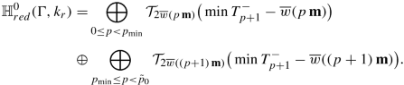
-
(d)
\({\mathrm {rank}\, } _{\mathbb Z} \mathbb H^0_{red}(\Gamma ,k_r)\) equals
$$\displaystyle \begin{aligned}\sum_{0\leq p<p_{\mathrm{min}}} \big(\min T^-_{p+1}-\overline{w}(p\,\mathbf{m})\big) + \sum_{p_{\mathrm{min}}\leq p<\tilde{p}_0} \big (\min T^-_{p+1}-\overline{w}((p+1)\,\mathbf{m})\big), \end{aligned}$$or
$$\displaystyle \begin{aligned} -m_{k_r}+ {\mathrm{rank}\, } _{\mathbb Z} \mathbb H^0_{red}(\Gamma,k_r)= \sum_{0\leq p<\tilde{p}_0} \big (\min T^-_{p+1}-\overline{w}((p+1)\,\mathbf{m})\big). \end{aligned}$$ -
(e)
For any q > 0 one has
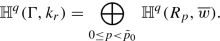


4.9.5 The Structure of \(\mathbb H^{\geq 1}(R_{p},\overline {w})\)
The cohomology \(\mathbb H^{\geq 1}(R_{p},\overline {w})\) depends only on the \(\overline {w}\)-values at p m, at (p + 1) m and along \(T^-_{p+1 }\). Indeed, for any \(n\in \mathbb Z\) consider Sn as in 4.5.2. Then for \(n< \min T^-_{p+1}\) the space Sn ∩ Rp has the same homotopy type as the intersection of Sn with the two-element set {p m, (p + 1) m}; while for \(n\geq \min T^-_{p+1}\) it has the homotopy type of the suspension of \(S_n\cap T^-_{p+1}\). In particular, all the nontrivial homogeneous elements of \(\mathbb H^{\geq 1}(R_{p},\overline {w})\) have degree \(\geq \min T^-_{p+1}\), and one has the graded \(\mathbb Z[U]\)-module isomorphism
4.9.6 The Structure of \(\mathbb H^{*}(T^-_{p+1},\overline {w})\). The Modules \(\mathbb H^{*}(\mathbb T^-_{n},\overline {W})\)
In most of the notations above, we have omitted the symbol a codifying the characteristic element kr. In fact, for any p ≥ 0 and a ∈{0, …, d − 1}, \(T^-_{p+1}\) is
Note that when p runs over \(\mathbb Z_{\geq 0}\) and a ∈{0, …, d − 1}, the integer n = pd + a runs over \(\mathbb Z_{\geq 0}\). This motivates to consider for any \(n\in \mathbb Z_{\geq 0}\)
Then, for d and a fixed, \(T^-_{p+1,a}=\mathbb T_{p d+a}+p\,\mathbf {m}\). If \(p<\tilde {p}_0\) then pd + a ≤ μ − 2, hence the relevant index set of the hyperplanes is 0 ≤ n ≤ μ − 2 (this can be compared with the index set \(\{\alpha _n\}_{n=0}^{\mu -2}\) of the coefficients of Q(t)). The form \(\mathbb T_{p d+a}+p\,\mathbf {m}\) shows also how they intersect the small rectangles: when we run a, an element of the set \(\{\mathbb T_{n}+\lfloor n/d\rfloor \mathbf {m}\}_{0\leq n\leq \mu -2}\) intersects Rp if and only if ⌊n∕d⌋ = p.
Up to the shift \(\overline {w}(p\,\mathbf {m})\), which is constant on each \(\mathbb T_n\), but otherwise depends on p = ⌊n∕d⌋, the weights on \(\mathbb T_n\cap \mathbb Z^\nu \) are given by the right hand side of (4.97). Or, up to a shift \(\overline {w}((p+1)\,\mathbf {m})\), the weights are given by (4.98). Following this second version we set the following weights for any \(\mathbb T_n\):
That is, \( \overline {W}|{ }_{\mathbb T_n}(\bar {l}-p\,\mathbf {m})= \overline {w}(\bar {l})-\overline {w}((p+1)\,\mathbf {m})\), where p = ⌊n∕d⌋.
The weight function \(\overline {W}\) restricted on all the level sets \(\{ \mathbb T_n\}_{n\geq 0}\) of \((\mathbb Z_{\geq 0})^\nu \) measures the very subtle distribution properties of the semigroups \(\{{\mathcal S}_i\}_i\). Furthermore, up to a well-identified shift in degrees, the collection \((\mathbb T_n,\overline {W})\) provides all the lattice cohomologies \(\mathbb H^*(\Gamma (d),k_r)\) for all the possible values d and a. Here, and in the next discussion, we denote the dependence of Γ on d by Γ(d).
More precisely, for any d and a ∈{0, …, d − 1} and q > 0 one has:

where sn,d is the value of the shift \(2\overline {w}((p+1)\,\mathbf {m})=2(p+1)(1+a-\delta )+d(p+1)p\) (with p = ⌊n∕d⌋). Moreover, the values \(\{\min \,\overline {W}\,|\mathbb T_n\}_n\) and sn,d determine all the cohomology groups \(\mathbb H^0(\Gamma (d), k_r)\) too. The second identity of (4.9.4)(d) together with (4.98) reads as:
In particular, for any fixed d > 0 and a ∈{0, …, d − 1} one has:
Example 4.9.7
For any d > 0 and q > 0 the summation of (4.102) over a gives

On the right hand side of (4.105) the numbers sn,d depend on d, but the rank of the right hand side is independent of d. In particular, up to shifts of different direct sum blocks, \(\oplus _{q>0}\mathbb H^q(\Gamma (d), k_r)\) is independent of the choice of the integer d. (This can also be deduced from the surgery exact sequences from [74].)
Example 4.9.8
-
(a)
Assume that for a certain d and a one gets \(\tilde {p}_0=0\). Then \(\mathbb H^*_{red}(\Gamma ,k_r)=0\), and \(\mathbb H^0(\Gamma ,k_r)={\mathcal T}^+_0\).
-
(b)
Assume that for a certain d and a one gets \(\tilde {p}_0=1\). Then \(\mathbb H^*(\Gamma ,k_r)=\mathbb H^*(R_0,\overline {w})\), hence everything is determined by \(T^-_{1,a}\). Indeed,
$$\displaystyle \begin{aligned} \min T^-_{1,a}=&\min\big\{ \sum_i \#\{s\in{\mathcal S}_i\,:\, s\leq \ell_i-1\}, \, \mbox{where }\sum_i\ell_i =a+1\,\big\}\\ =&\min\big\{ \sum_i \#\{s\nless xx>\in{\mathcal S}_i\,:\, s\geq \ell_i\}, \, \mbox{where }\sum_i\ell_i=a+1\,\big\} +1+a-\delta, \end{aligned}$$\(m_{k_r}=\min \{0,1+a-\delta \},\) \(\mathbb H^0_{red}(\Gamma ,k_r)\) is generated by one element of degree \(2\max \{0, 1+a-\delta \}\), \(\mathrm {rank}\, \,\mathbb H^0_{red}(\Gamma ,k_r)= \min \, T^-_{1,a} -\max \{0, 1+a-\delta \}\), and finally for q > 0 one has \(\mathbb H^q(\Gamma ,k_r)=\mathbb H^{q-1}_{red}(T^-_{1,a},\overline {w})= \mathbb H^{q-1}_{red}({\mathbb T}_a,\overline {W})[2(1+a-\delta )]\), (\(T^-_{1,a}={\mathbb T}_a+\mathbf {m}\)).
-
(c)
If d ≥ μ − 1 then \(\tilde {p}_0=1\) for a < μ − 1, and \(\tilde {p}_0=0\) for a ≥ μ − 1.
Remark 4.9.9
Assume that we know all the cohomology groups \(\{\mathbb H^*(\Gamma (d),k_r)\}_{k_r}\) for some specific d with d ≥ μ − 1. Then using them, and also the values \(\overline {w}(p\mathbf {m}) = p(1+a-\delta )+dp(p-1)/2\) for all p, a and d, we can recover all the lattice cohomologies \(\{\mathbb H^*(\Gamma (d),k_r)\}_{k_r}\) for any d > 0. [For this, use Example 4.9.8 and (4.102).]
Corollary 4.9.10
For any n ≥ 0 the coefficients of Q(t) =∑n αn tn satisfy
Proof
Use the identities (4.93) and (4.104) for d ≫ 0, cf. 4.9.9. □
Remark 4.9.11
Above we reduced several computations to the weight function \(\overline {W}|{ }_{{\mathbb T}_n}\). It was connected with the weight function provided by the reduction formula via \( \overline {W}|{ }_{\mathbb T_n}(\bar {l}-p\,\mathbf {m})= \overline {w}(\bar {l})-\overline {w}((p+1)\,\mathbf {m})\), where p = ⌊n∕d⌋. Since each \(\overline {w}(p\,\mathbf {m})\) is computable from d, a, δ, cf. 4.9.3 (b), the lattice cohomology \(\mathbb {H}^0(S^3_{-d}(\#_iK_i))\) is computable from d, a, δ and \(\{\overline {W}|{ }_{{\mathbb T}_n}\}_n\). On the other hand, by (4.101) \( \overline {W}((\ell _{1,0},\ldots ,\ell _{\nu ,0}))\) equals \(\sum _i\, \#\{s \not \in {\mathcal S}_i\,:\, s\geq \ell _{i,0}\} = \sum _i\left ( \delta _i-\# \{s_i\not \in {\mathcal S}_i: s_i<\ell _{i,0}\}\right )= \sum _i ( \delta _i -\ell _{i,0}) + \sum _i \#\{s_i\in {\mathcal S}_i: s_i<\ell _{i,0}\}\). Hence
This motivates the replacement of the semigroup \({\mathcal S}_i\) with an equivalent object of it, with its ‘counting function’ j↦Hi(j),
From analytic point of view, Hi(j) is the coefficient of tj in the Hilbert function of the local singularity (C, pi), associated with the filtration given by its normalization.
The above min-expression can be reformulated formally as follows. Consider any two functions H1 and H2 defined on integers and bounded from below. Then we define their ‘minimum convolution’ (cf. [9, 5.3]), denoted by H1 ◇ H2 as \( (H_1 \diamond H_2)(j) = \min _{j_1+j_2=j}\{ H_1(j_1) + H_2(j_2) \}\).
Then from the counting functions \(\{H_i\}_{i=1}^\nu \) associated with \(\{{\mathcal S}_i\}_{i=1}^\nu \) we construct
Since the operator ◇ is associative and commutative, the function H is well-defined.
From the above discussion \(\mathbb {H}^0(S^3_{-d}(\#_iK_i))\) is computable from d, a, δ and H.
Remark 4.9.12
In the above discussion (e.g. in 4.9.5–4.9.6), the space \(\mathbb T_n\)—intersection of a simplex with a rectangle—can be replaced by the supporting simplex. Indeed, set
A verification shows that \(H^*_{red}(\mathbb T_n,\overline {W})\) is isomorphic with \(H^*_{red}(\Sigma _n,\overline {W})\) for every n ≥ 0. Furthermore, if n > μ − 2 then \(H^*_{red}(\mathbb T_n,\overline {W})=0\) automatically, hence in several formulae above (e.g. in the summations from (4.102) and (4.105)) the restrictions n ≤ μ − 2 can be safely neglected.
4.9.2 Superisolated Singularities with More Cusps
In this subsection we consider a superisolated singularity associated with an irreducible rational cuspidal curve. For different notations and statements regarding the analytic and topological type see Sects. 4.2.4, 4.3.6, 4.4.11, 4.7.4, and 4.9. In this subsection we follow [8].
Our goal is to discuss Conjectures 4.3.21 and 4.3.22 from the point of view of lattice cohomology. Let us recall the two statements. Set (cf. 4.3.20 (b))
-
Conjecture 4.3.21: all the coefficients of N(t) are non-positive. We will refer to this as ‘Conjecture C’ (‘Conjecture regarding the coefficients of N(t)’).
-
Conjecture 4.3.22: N(1) is non-positive. We will refer to this as the ‘Conjecture I’ (we regard N(1) as an ‘index type invariant’).
Clearly Conjecture C implies Conjecture I.
We will compare these statements with the Semigroup Distribution Property based on the properties of counting function Hi of the semigroups and also on a subtle connection with lattice cohomology.
We consider the counting functions Hi of the semigroups \({\mathcal S}_{i}\) (cf. (4.108)) and their minimum convolution H as in (4.109). Recall also (cf. 4.2.33) that the Semigroup Distribution Property (SDP) reads as H(ld + 1) = (l + 1)(l + 2)∕2 for any l = 0, 1, …d − 3.
Example 4.9.13 (The case ν = 1)
In this case \(\alpha _j=\#\{s\not \in {\mathcal S}_{1}: s>j\}\), cf. (4.42). From (4.43) α2δ−2−j = H1(j + 1) for j = 0, …, 2δ − 2. Hence, the α-coefficient needed in (4.111) is \(\alpha _{(d-3-l)d}=\#\{s\in {\mathcal S}_{1}\, :\, s\leq ld\}=H_1(ld+1)\). Recall that 4.2.33 (Bézout’s Theorem) implies α(d−3−l)d = H1(ld + 1) ≥ (l + 1)(l + 2)∕2. This inequality and (4.111) show that for ν = 1 Conjecture C is equivalent to N(t) ≡ 0. But, they are also equivalent to Conjecture I, since if N(1) ≤ 0 then necessarily N(t) ≡ 0. Finally, the validity of all these statements follow from SDP.
However, for ν ≥ 2 the relationships are more subtle.
Theorem 4.9.14 ([8])
With the above notations one has:
-
1.
If ν = 2, then q2δ−2−j ≤ H(j + 1) for any j = 0, 1, …2δ − 2. Therefore, for bicuspidal curves the SDP implies Conjecture C (hence Conjecture I too).
-
2.
If ν ≥ 3, then the inequality q2δ−2−j ≤ H(j + 1) does not hold in general, not even for j = ld (l = 0, 1, …, d − 3), needed for Conjectures C and I. Moreover, Conjecture C is not true in general, and Conjecture I behaves independently from SDP. (Conjecture I remains as a conjecture, though its validity is verified directly for all ‘known’ curves.)
For a direct elementary proof of part (1) see [65].
4.9.15 Combinatorial Reformulations
The next discussion aims to clarify the similarities and differences between the polynomial Q and the function H.
Let us start with ν semigroups \(\{{\mathcal S}_{i}\}_{i=1}^\nu \) associated with local irreducible plane curve singularities. However, in the next discussion we will not require their realizability as singularities of a projective rational curve. [Regarding the realizability, we use the following terminology. If the sum δ of delta-invariants of the local singularity types is of form 2δ = (d − 1)(d − 2) for some integer d, then we say that these ν local topological types are combinatorial candidates for the ν singularities of a rational cuspidal plane curve of degree d. If such a curve really exists then (SDP) is valid for the corresponding local data and d.],
The semigroups determine their counting functions Hi by (4.108) and the minimal convolution H of the functions {Hi}i by (4.109). For convenience, define also the sequences \(\{h^{(i)}_j\}_{j=0}^{\infty }\) by \(h^{(i)}_j := H_i(j+1)\).
For any sequence \(a = \{a_j\}_{j=0}^{\infty }\) denote by ∂a its difference sequence, i.e. (∂a)j = aj − aj−1 with the convention a−1 = 0. Similarly, we will denote by Σa the sequence of partial sums, i.e. ( Σa)j = a0 + ⋯ + aj. Of course, Σ∂a = a and ∂ Σa = a for any sequence a.
By (4.108) and  (cf. (4.6) the coefficient \(c^{(i)}_j\) of tj in
  can be written as \(c^{(i)}_j = (\partial \partial h^{(i)})_j\). The coefficient sequence of a polynomial product is the usual convolution of coefficient sequences of the factors. Hence, the coefficient cj of tj in
  is \(c_j = \sum _{j_1 + \dots + j_{\nu } = j} c^{(1)}_{j_1} \cdots c^{(\nu )}_{j_{\nu }}\). Denoting the convolution of two sequences \(a = \{a_j\}_{j=0}^{\infty }\) and \(b = \{b_j\}_{j=0}^{\infty }\) by a ∗ b, i.e. \((a \ast b)_j = \sum _{k=0}^ja_kb_{j-k}\), we get cj = (∂∂h(1) ∗⋯ ∗ ∂∂h(ν))j. Let us define:
Before we identify F, let us recall some symmetry properties. From the symmetry of  (and from δ =∑i
δi)
(and from δ =∑i
δi)
This (or the symmetry of each semigroup) implies also Hi(ji) = Hi(2δi − ji) + ji − δi, from which one also obtains
Next, if A(t) =∑j
aj
tj and B(t) =∑j
bj
tj satisfy A(t) = A(1) + (t − 1)B(t), then ( Σa)j = A(1) − bj. This applied twice for  gives ( Σ Σc)j = j + 1 − δ + αj. Hence, then the definition of Q and (4.113) provide
In other words, the H-values are obtained from {h(i)}i by minimal convolution (shifted by one), while the F-coefficients (or α-coefficient in opposite order) are obtained by the composition of ∂∂, the usual convolution, and the Σ Σ operator.
Then one has the following reinterpretations in terms of F and H.
Let \(C \subset \mathbb {C}P^2\) be a rational cuspidal curve of degree d with ν cusps of given topological types (in particular, d(d − 3) = 2δ − 2). Set F(j) := ( Σ Σ(∂∂h(1) ∗⋯ ∗ ∂∂h(ν)))j, where \(h^{(i)}_j=H_i(j+1)\), and Hi is the semigroup counting function of the i-th singularity. Set H := H1 ◇⋯ ◇ Hν. Then
Let us summarize the combinatorial situation. Starting from the semigroups of ν local singularities we define H and F.
If ν = 1 (since Σ Σ∂∂(h) = h) then F(j) = H(j + 1) for each \(j\in \mathbb Z_{\geq 0}\) (independently of realizability, hence not just for \(j\in d \cdot \mathbb Z_{\geq 0}\)).
On the other hand, for ν > 1 the values F(j) and H(j + 1) become different. Nevertheless, cf. Theorem 4.9.14 (1) F(j) ≤ H(j + 1) remains true for ν = 2 and every integer j ≥ 0, again by combinatorial (lattice cohomology) argument (independently of realizability and d).
With these facts in mind, it is tempting to conjecture that maybe the inequality F(j) ≤ H(j + 1) is always true—as a property of local singularity types—, which would make Conjecture C a combinatorial corollary of SDP. But, for ν ≥ 3 there is no such relation between the local functions F and H.
4.9.16 Lattice Cohomological Reinterpretation
Consider the combinatorial situation from 4.9.15. The semigroups \({\mathcal S}_{i}\) determine links Ki ⊂ S3 of the corresponding (topological types) of plane curve singularities. Consider an arbitrary d > 0 and the surgery 3-manifold \(S^3_{-d}(\#_iK_i)\) as in Sect. 4.9.
The next statements show a remarkable common feature of the functions F and H.
Theorem 4.9.17
For any d > 0 and 0 ≤ a < d the following facts hold:
Proof
We will use the identities from (4.104). In the first one, note that by (4.101), (4.100), and (4.107) \(\min (\overline {W}|{ }_{{{\mathbb T}_j}})\) is δ − j − 1 + H(j + 1) and (4.119) follows (for its second identity use (4.114)).
For the second identity, note that \(-eu(\mathbb H^*({\mathbb T}_j, \overline {W})\) equals αj by (4.106), which is F(2δ − 2 − j) by (4.115). Then use again the symmetry (4.113). □
Remark 4.9.18
In fact, by Theorem 4.9.4, the integer d, the sum of delta-invariants δ and the function H completely determine the whole \(\mathbb {H}^0\) as a graded \(\mathbb {Z}[U]\)-module (and not just its Euler characteristic).
Corollary 4.9.19
Assume that d(d − 3) = 2δ − 2 (that is, d and \(\{{\mathcal S}_i\}_i\) constitute a package of combinatorial candidates for algebraic realizability). Then
This for a = 0 reads as
Since by 4.2.33 H(ld + 1) ≥ (l + 1)(l + 2)∕2 for any l = 0, …, d − 3, \(\sum _{l=0}^{d-3}H(ld+1)=\sum _{l=0}^{d-3} (l+1)(l+2)/2\) is equivalent to SDP for every l (cf. (4.118)). In particular, in the presence of the algebraic realization, the valid SDP reads as:
Furthermore, under the same realizability assumption, Conjecture I reads as:
They combined:
4.9.20 Proof of Conjecture I for ν = 2 (via SDP)
First note that \({\mathbb H}^q(S^3_{-d}(\#_iK_i),k_r)=0\) for any q ≥ ν and any kr (cf. 4.8.3). Then, for ν = 2, one has \(eu \left ( \mathbb {H}^* (S^3_{-d}(\#_iK_i),K)\right ) = eu \left ( \mathbb {H}^0 (S^3_{-d}(\#_iK_i),K)\right )- \mathrm {rank} _{\mathbb Z}\mathbb {H}^1 (S^3_{-d}(\#_iK_i),K)\), hence (4.123) follows.
For ν ≥ 3 the similar argument does not work. From this point of view, it is even more surprising that in all the known cases Conjecture I still holds, cf. 4.9.14.
4.10 Lattice Cohomology and Heegaard Floer Homology
The Seiberg–Witten invariant is the (normalized) Euler-characteristic of the Seiberg–Witten monopole Floer homology of Kronheimer–Mrowka, or equivalently, of the Heegaard Floer homology of Ozsváth and Szabó. These theories had an extreme influence on the modern mathematics, solving (or disproving) a long list of old conjectures (e.g. Thom Conjecture, or conjectures regarding classification of 4-manifolds, or famous old problems in knot theory); see the long list of distinguished articles of Kronheimer–Mrowka or Ozsváth–Szabó. In [102] Ozsváth and Szabó provided a computation of the Heegaard Floer homology for some special plumbed 3-manifolds. This computation resonated incredibly with the theory of computation sequences used in Artin–Laufer program (see e.g. [50, 67, 68]). These two facts influenced considerably the definition of the lattice cohomology.
4.10.1 The Conjecture Connecting Lattice Cohomology and Heegaard Floer Theory
4.10.1 Short Review of Heegaard Floer Homology HF+(M)
We assume that M is an oriented rational homology 3–sphere, and we restrict ourselves to the +–theory of Ozsváth and Szabó. The Heegaard Floer homology HF+(M) is a \(\mathbb Z[U]\)–module with a \(\mathbb {Q}\)–grading compatible with the \(\mathbb Z[U]\)–action, where deg(U) = −2. Additionally, HF+(M) has another \(\mathbb Z_2\)–grading; HF+(M)even, respectively HF+(M)odd denote the graded parts. Moreover, HF+(M) has a natural direct sum decomposition of \(\mathbb Z[U]\)–modules (compatible with all the gradings): HF+(M) = ⊕σ HF+(M, σ) indexed by the spinc structures σ of M. For any σ ∈Spinc(M) one has
a graded \(\mathbb Z[U]\)–module isomorphism, and \(HF^+_{red}(M,\sigma )\) has finite \(\mathbb Z\)–rank and an induced \(\mathbb Z_2\)–grading. One also considers
Then the Seiberg–Witten invariant of (M, σ) equals χ(HF+(M, σ)) − d(M, σ)∕2.
By changing the orientation we have χ(HF+(M, σ)) = −χ(HF+(−M, σ)) and d(M, σ) = −d(−M, σ).
4.10.2 The Predicted Connection
In [72] the author formulated the following
Conjecture 4.10.3
For any plumbed rational homology sphere associated with a connected negative definite graph Γ, and for any k ∈Char, one has
Furthermore,

and

Both parts of the Conjecture were verified for almost rational graphs in [72], for two bad vertices in [101], see [72, 8.4] too. Otherwise, the Conjecture is still open.
Note that (conjecturally) \(\mathbb H^*\) has a richer structure: its q–filtration \(\mathbb H^*=\oplus _q\,\mathbb H^q\) collapses at the level of HF+ to a \(\mathbb Z_2\) odd/even filtration.
The fact that both theories have the same Euler characteristic support the above conjecture as well. Another supporting evidence is the following fact.
4.10.4 Coincidence of the Vanishing of the Reduced Theories
By 4.6.22 the graph Γ is rational if and only if \(\mathbb H^*_{red}(\Gamma )=0\). On the other hand, following Ozsváth and Szabó, by definition, M is an L–space if and only if \(HF^+_{red}=0\). Their equivalence is predicted by Conjecture 4.10.3. This ‘tip of the iceberg’ statement was proved in [76]:
Theorem 4.10.5
The following facts are equivalent for a connected negative definite graph Γ:
-
(i)
Γ is a rational graph,
-
(ii)
M = M( Γ) is an L–space.
(i) ⇒ (ii) follows from lattice cohomology theory [70, 72], while (ii) ⇒ (i) uses partly the following equivalence (ii) ⇔ (iii), where (iii) means that π1(M) is not a left-orderable group. [A non trivial group G is said to be left-orderable if there exist a total order < on G such that if a < b then ga < gb for every g ∈ G.] The equivalence (ii) ⇔ (iii) was proved in [33] for any graph–manifold. For arbitrary 3–manifolds it was conjectured by Boyer, Gordon and Watson [10], for different developments and other references see [33, 76].
Problem 4.10.6
Characterize elliptic singularities (or other non-rational families of singularities) by a certain property of the fundamental group of the link.
References
Norbert A’Campo. Sur la monodromie des singularités isolées d’hypersurfaces complexes. Inventiones mathematicae, 20, 1973.
Selman Akbulut and John D. McCarthy. Casson’s Invariant for Oriented Homology Three-Spheres. Mathematical Notes. Princeton University Press, 1990.
Enrique Artal-Bartolo. Forme de Jordan de la monodromie des singularités superisolées de surfaces. Memoirs of the Amer. Math. Soc., 109, 1994.
Enrique Artal-Bartolo, Pierre Cassou-Noguès, Ignacio Luengo, and Alejandro Melle-Hernández. Monodromy conjecture for some surface singularities. Ann. Sci. de l’École Norm. Sup., 35, 2002.
Michael Artin. Some numerical criteria for contractability of curves on algebraic surfaces. American Journal of Mathematics, 84, 1962.
Michael Artin. On isolated rational singularities of surfaces. American Journal of Mathematics, 88, 1966.
Wolf P. Barth, Chris A. M. Peters, and Antonius Van de Ven. Compact complex surfaces. Ergebnisse der Mathematik und ihrer Grenzgebiete. Springer-Verlag, 1984.
József Bodnár and András Némethi. Lattice cohomology and rational cuspidal curves. Mathematical Research Letters, 23, 2016.
Maciej Borodzik and Charles Livingston. Heegaard Floer homology and rational cuspidal curves. Forum of Mathematics, Sigma, 2, 2014.
Steven Boyer, C. McA. Gordon, and L Watson. On L–spaces and left-orderable fundamental groups. Mathematische Annalen, 356, 2013.
Steven Boyer and Andrew Nicas. Varieties of group representations and Casson’s invariant for rational homology 3-spheres. Transactions of the Amer. Math. Soc., 322, 1990.
Gábor Braun and András Némethi. Surgery formula for Seiberg–Witten invariants of negative definite plumbed 3-manifolds. Journal für die reine und ang. Math., 2010, 2009.
Winfried Bruns and Jürgen Herzog. Cohen–Macaulay Rings. Cambridge Studies in Advanced Mathematics. Cambridge University Press, 1998.
Dan Burghelea and Andrei Verona. Local homological properties of analytic sets. Manuscripta Mathematica, 7, 1972.
Antonio Campillo, Félix Delgado, and Sabir M. Gusein-Zade. On the monodromy of a plane curve singularity and the Poincaré series of the ring of functions on the curve. Functional Analysis and Its Applications, 33, 1999.
Patrick du Val. On absolute and non-absolute singularities of algebraic surfaces. Rev. de la Fac. des Sci. de l’Univ. d’Istanbul, Série A, 9, 1944.
Alan H. Durfee. The signature of smoothings of complex surface singularities. Mathematische Annalen, 232, 1978.
Alan H. Durfee. Neighborhoods of algebraic sets. Transactions of the Amer. Math. Soc., 276, 1983.
David Eisenbud and Walter David Neumann. Three-Dimensional Link Theory and Invariants of Plane Curve Singularities. Annals of Mathematics Studies. Princeton University Press, 1985.
Hélène Esnault. Reflexive modules on quotient surface singularities. Journal für die reine und ang. Math., 1985, 1985.
Hélène Esnault and Eckart Viehweg. Two dimensional quotient singularities deform to quotient singularities. Mathematische Annalen, 271, 1985.
Hélène Esnault and Eckart Viehweg. Lectures on Vanishing Theorems. DMV Seminar. Birkhäuser, 1992.
Javier Fernández de Bobadilla, Ignacio Luengo, Alejandro Melle-Hernández, and András Némethi. Classification of Rational Unicuspidal Projective Curves whose Singularities Have one Puiseux Pair. Trends in Mathematics. Birkhäuser, 2006.
Javier Fernández de Bobadilla, Ignacio Luengo, Alejandro Melle-Hernández, and András Némethi. On rational cuspidal projective plane curves. Proc. of the London Math. Soc., 92, 2006.
Javier Fernández de Bobadilla, Ignacio Luengo, Alejandro Melle-Hernández, and András Némethi. On rational cuspidal curves, open surfaces and local singularities. World Scientific, 2007.
Ronald Fintushel and Ronald John Stern. Instanton homology of Seifert fibred homology three spheres. Proc. of the London Math. Soc., s3-61, 1990.
Shinji Fukuhara and Noriko Maruyama. A sum formula for Casson’s λ-invariant. Tokyo Journal of Mathematics, 11, 1988.
Hans Grauert. Über Modifikationen und exzeptionelle analytische Mengen. Mathematische Annalen, 146, 1962.
Hans Grauert and Reinhold Remmert. Zur theorie der Modifikationen. I. Stetige und eigentliche Modifikationen komplexer Räume. Mathematische Annalen, 129, 1955.
Hans Grauert and Reinhold Remmert. Coherent Analytic Sheaves. Grundlehren der mathematischen Wissenschaften. Springer-Verlag, 1984.
Hans Grauert and Oswald Riemenschneider. Verschwindungssätze für analytische kohomologiegruppen auf komplexen Räumen. Inventiones mathematicae, 11, 1970.
Helmut Arend Hamm. Die topologie isolierter Singularitäten von vollständigen Durchschnitten komplexer Hyperflächen. PhD thesis. Rheinische Friedrich-Wilhelms-Universität Bonn, 1969.
J Hanselman, J Rassmussen, S Rasmussen, and L Watson. L–spaces, taut foliations, and graph manifolds. Compositio Mathematica, 156, 2020.
Robin Hartshorne. Algebraic Geometry. Graduate Texts in Mathematics. Springer-Verlag, 1977.
Friedrich Hirzebruch. Über vierdimensionale Riemannsche Flächen mehrdeutiger analytischer Funktionen von zwei komplexen Veränderlichen. Mathematische Annalen, 126, 1953.
Friedrich Hirzebruch. Hilbert modular surfaces. L’Enseignement Mathématique, 19, 1973.
Friedrich Hirzebruch, Sebastian Su Koh, and Walter David Neumann. Differentiable manifolds and quadratic forms. Lecture Notes in Pure and Appl. Math. Marcel Dekker, 1971.
William Jaco. Lectures on Three-Manifold Topology. CBMS Regional Conference Series in Mathematics. American Mathematical Society, 1980.
Mark Jankins and Walter David Neumann. Lectures on Seifert Manifolds. Brandeis Lecture Notes. American Mathematical Society, 1983.
Heinrich Wilhelm Ewald Jung. Darstellung der Funktionen eines algebraischen Körpers zweier unabhängigen Veränderlichen x, y in der Umgebung einer Stelle x = a, y = b. Journal für die reine und ang. Math., 1908, 1908.
Heinrich Wilhelm Ewald Jung. Einführung in die Theorie der algebraischen Funktionen zweier Veränderlicher. Akademie-Verlag, 1951.
János Kollár. Shafarevich Maps and Automorphic Forms. Princeton University Press, 1995.
János Kollár. Lectures on Resolution of Singularities. Annals of Mathematics Studies. Princeton University Press, 2007.
Tamás László. Lattice cohomology and Seiberg–Witten invariants of normal surface singularities. PhD thesis. Central European University, Budapest, 2013.
Tamás László, János Nagy, and András Némethi. Surgery formulae for the Seiberg–Witten invariant of plumbed 3-manifolds. Revista Matemática Complutense, 33, 2020.
Tamás László and András Némethi. Ehrhart theory of polytopes and Seiberg–Witten invariants of plumbed 3-manifolds. Geometry & Topology, 18, 2014.
Tamás László and András Némethi. Reduction theorem for lattice cohomology. Int. Math. Research Notices, 2015, 2015.
Henry Ben Laufer. Normal Two-Dimensional Singularities. Annals of Mathematics Studies. Princeton University Press, 1972.
Henry Ben Laufer. On rational singularities. American Journal of Mathematics, 94, 1972.
Henry Ben Laufer. On minimally elliptic singularities. American Journal of Mathematics, 99, 1977.
Henry Ben Laufer. On μ for surface singularities. Proc. of Symposia in Pure Mathematics. American Mathematical Society, 1977.
Henry Ben Laufer. Weak simultaneous resolution for deformations of Gorenstein surface singularities. Proc. of Symposia in Pure Mathematics. American Mathematical Society, 1983.
Henry Ben Laufer. The multiplicity of isolated two-dimensional hypersurface singularities. Transactions of the Amer. Math. Soc., 302, 1987.
Dũng Tráng Lê. Singularités isolées des intersections complètes. Travaux en Cours. Hermann, 1997.
Christine Lescop. Global Surgery Formula for the Casson–Walker Invariant. Annals of Mathematics Studies. Princeton University Press, 1996.
Joseph Lipman. Rational singularities, with applications to algebraic surfaces and unique factorization. Publ. Math. de l’IHÉS, 36, 1969.
Joseph Lipman. Introduction to resolution of singularities. Proc. of Symposia in Pure Mathematics. American Mathematical Society, 1975.
Stanisław Łojasiewicz. Triangulation of semi-analytic sets. Ann. della Scuola Norm. Sup. di Pisa, Classe di Sci., 18, 1964.
Eduard Jacob Neven Looijenga. Isolated Singular Points on Complete Intersections. London Math. Soc. Lecture Note Series. Cambridge University Press, 1984.
Ignacio Luengo. The μ-constant stratum is not smooth. Inventiones mathematicae, 90, 1987.
Ignacio Luengo, Alejandro Melle-Hernández, and András Némethi. Links and analytic invariants of superisolated singularities. Journal of Algebraic Geometry, 14, 2005.
Alejandro Melle-Hernández. Milnor numbers for surface singularities. Israel Journal of Mathematics, 115, 2000.
John Milnor. Singular Points of Complex Hypersurfaces. Annals of Mathematics Studies. Princeton University Press, 1969.
David Mumford. The topology of normal surface singularities of an algebraic surface and a criterion of simplicity. Publ. Math. de l’IHÉS, 9, 1961.
Piotr Nayar and Barbara Piłat. A note on the rational cuspidal curves. Bulletin of the Polish Acad. of Sci. Math., 62, 2014.
András Némethi. Normal surface singularities, (book in preparation). To appear in Springer series Ergebnisse der Mathematik und ihrer Grenzgebiete.
András Némethi. Five Lectures on Normal Surface Singularities. Bolyai Society Mathematical Studies. János Bolyai Mathematical Society, 1999.
András Némethi. Invariants of normal surface singularities. Contemporary Mathematics. American Mathematical Society, 2004.
András Némethi. On the Heegaard Floer homology of \(S^3_{-d}(K)\) and unicuspidal rational plane curves. Fields Institute Communications. American Mathematical Society, 2005.
András Némethi. On the Ozsváth–Szabó invariant of negative definite plumbed 3-manifolds. Geometry & Topology, 9, 2005.
András Némethi. Graded roots and singularities. World Scientific, 2007.
András Némethi. Lattice cohomology of normal surface singularities. Publ. of the Res. Inst. for Math. Sci., 44, 2008.
András Némethi. The Seiberg–Witten invariants of negative definite plumbed 3-manifolds. Journal of the Eur. Math. Soc., 13, 2011.
András Némethi. Two exact sequences for lattice cohomology. Contemporary Mathematics. American Mathematical Society, 2011.
András Némethi. The cohomology of line bundles of splice-quotient singularities. Advances in Mathematics, 229, 2012.
András Némethi. Links of rational singularities, L-spaces and lo fundamental groups. Inventiones mathematicae, 210, 2017.
András Némethi. Pairs of invariants of surface singularities. Proc. Int. Cong. of Math., Rio de Janeiro, 1, 2018.
András Némethi and Liviu I. Nicolaescu. Seiberg–Witten invariants and surface singularities. Geometry & Topology, 6, 2002.
András Némethi and Liviu I. Nicolaescu. Seiberg–Witten invariants and surface singularities ii: Singularities with good \(\mathbb {C}^*\)-action. Journal of the London Math. Soc., 69, 2004.
András Némethi and Liviu I. Nicolaescu. Seiberg–Witten invariants and surface singularities: splicings and cyclic covers. Selecta Mathematica, New Series, 11, 2006.
András Némethi and Tomohiro Okuma. The Seiberg–Witten invariant conjecture for splice-quotients. Journal of the London Math. Soc., 78, 2008.
András Némethi and Tomohiro Okuma. On the Casson invariant conjecture of Neumann–Wahl. Journal of Algebraic Geometry, 18, 2009.
András Némethi and Tomohiro Okuma. The embedding dimension of weighted homogeneous surface singularities. Journal of Topology, 3, 2010.
András Némethi and Fernando Román. The lattice cohomology of \(S^3_{-d}(K)\). Contemporary Mathematics. American Mathematical Society, 2012.
András Némethi and Baldur Sigurðsson. The geometric genus of hypersurface singularities. Journal of the Eur. Math. Soc., 18, 2016.
András Némethi and Baldur Sigurðsson. Local Newton nondegenerate Weil divisors in toric varieties. 2021.
Walter David Neumann. A calculus for plumbing applied to the topology of complex surface singularities and degenerating complex curves. Transactions of the Amer. Math. Soc., 268, 1981.
Walter David Neumann. Abelian covers of quasihomogeneous surface singularities. Proc. of Symposia in Pure Mathematics. American Mathematical Society, 1983.
Walter David Neumann and Frank Raymond. Seifert manifolds, plumbing, μ-invariant and orientation reserving maps. Lecture Notes in Mathematics. Springer-Verlag, 1978.
Walter David Neumann and Jonathan Wahl. Casson invariants of links of singularities. Commentarii Mathematici Helvetici, 65, 1990.
Walter David Neumann and Jonathan Wahl. Complete intersection singularities of splice type as universal abelian covers. Geometry & Topology, 9, 2005.
Walter David Neumann and Jonathan Wahl. Complex surface singularities with integral homology sphere links. Geometry & Topology, 9, 2005.
Walter David Neumann and Jonathan Wahl. The end curve theorem for normal complex surface singularities. Journal of the Eur. Math. Soc., 12, 2010.
Liviu I. Nicolaescu. The Reidemeister Torsion of 3-Manifolds. De Gruyter Studies in Mathematics. De Gruyter, 2003.
Liviu I. Nicolaescu. Seiberg–Witten invariants of rational homology 3-spheres. Communications in Contemp. Math., 6, 2004.
Tomohiro Okuma. Universal abelian covers of rational surface singularities. Journal of the London Math. Soc., 70, 2004.
Tomohiro Okuma. The geometric genus of splice-quotient singularities. Transactions of the Amer. Math. Soc., 360, 2008.
Tomohiro Okuma. Another proof of the end curve theorem for normal surface singularities. Journal of the Math. Soc. of Japan, 62, 2010.
Peter Orlik and Philip Wagreich. Isolated singularities of algebraic surfaces with \(\mathbb {C}^*\)-action. Annals of Mathematics, 93, 1971.
Peter Orlik and Philip Wagreich. Singularities of algebraic surfaces with \(\mathbb {C}^*\)-action. Mathematische Annalen, 193, 1971.
Peter Ozsváth, András I. Stipsicz, and Zoltán Szabó. A spectral sequence on lattice cohomology. Quantum Topology, 5.
Peter Ozsváth and Zoltán Szabó. On the Floer homology of plumbed three-manifolds. Geometry & Topology, 7, 2003.
Henry Charles Pinkham. Normal surface singularities with \(\mathbb {C}^*\)-action. Mathematische Annalen, 227, 1977.
Chakravarthi Padmanabhan Ramanujam. Remarks on the Kodaira vanishing theorem. Journal of the Indian Math. Soc., 36, 1972.
Oswald Riemenschneider. Deformationen von Quotientensingularitäten (nach zyklischen Gruppen). Mathematische Annalen, 209, 1974.
Oswald Riemenschneider. Zweidimensionale Quotientensingularitäten: Gleichungen und Syzygien. Archiv der Mathematik, 37, 1981.
Alois Scharf. Zur Faserung von Graphenmannigfaltigkeiten. Mathematische Annalen, 215, 1975.
Herbert Seifert. Topologie dreidimensionaler gefaserter Räume. Acta Mathematica, 60, 1933.
Jean-Pierre Serre. A Course in Arithmetic. Graduate Texts in Mathematics. Springer-Verlag, 1973.
Karl Stein. Analytische Zerlegungen komplexer Räume. Mathematische Annalen, 132, 1956.
Jan Stevens. Universal abelian covers of superisolated singularities. Mathematische Nachrichten, 282, 2009.
Masataka Tomari and Keiichi Watanabe. Normal \(\mathbb {Z}_r\)-graded rings and normal cyclic covers. Manuscripta Mathematica, 76, 1992.
Masataka Tomari and Keiichi Watanabe. Cyclic covers of normal graded rings. Kodai Mathematical Journal, 24, 2001.
Vladimir Turaev. Introduction to Combinatorial Torsions. Lectures in Mathematics ETH Zürich. Birkhäuser, 2001.
Vladimir Turaev. Torsions of 3-Dimensional Manifolds. Progress in Mathematics. Birkhäuser, 2002.
Kevin Walker. An Extension of Casson’s Invariant. Annals of Mathematics Studies. Princeton University Press, 1992.
Edward Witten. Monopoles and four-manifolds. Mathematical Research Letters, 1, 1994.
Oscar Zariski. The reduction of the singularities of an algebraic surface. Annals of Mathematics, 40, 1939.
Oscar Zariski. A simplified proof for the resolution of singularities of an algebraic surface. Annals of Mathematics, 43, 1942.
Oscar Zariski. Foundations of a general theory of birational correspondences. Transactions of the Amer. Math. Soc., 53, 1943.
Acknowledgements
The author was supported by the NKFIH Grant KKP 126683.
Author information
Authors and Affiliations
Corresponding author
Editor information
Editors and Affiliations
Rights and permissions
Copyright information
© 2022 Springer Nature Switzerland AG
About this chapter

Cite this chapter
Némethi, A. (2022). Surface Singularities, Seiberg–Witten Invariants of Their Links and Lattice Cohomology. In: Cisneros-Molina, J.L., Dũng Tráng, L., Seade, J. (eds) Handbook of Geometry and Topology of Singularities III. Springer, Cham. https://doi.org/10.1007/978-3-030-95760-5_4
Download citation
DOI: https://doi.org/10.1007/978-3-030-95760-5_4
Published:
Publisher Name: Springer, Cham
Print ISBN: 978-3-030-95759-9
Online ISBN: 978-3-030-95760-5
eBook Packages: Mathematics and StatisticsMathematics and Statistics (R0)