
Abstract
This paper presents a case study of using a digital twin model to control and monitor a real industrial robot. The digital twin and user interfaces are designed and implemented in the Unity 3D environment. The inverse kinematics of the robot is analytically calculated. Both the digital twin and the physical model (the robot Mitsubishi RV-12SD) is successfully integrated, and the data flow can be exchanged one another to control both the models to work together. The real system integration and the collaborating scenarios demonstrate the potential and advantage of the proposed method to develop a smarter programming, controlling and monitoring system for industrial robots.
Access provided by Autonomous University of Puebla. Download conference paper PDF
Keywords
1 Introduction
In recent years, the welding robot plays an important role in several manufacturing industries such as automotive industry, shipbuilding industry, etc. The use of the welding robot for welding complex mechanical parts is to increase the productivity of the production and reduce the use of manpower for manufacturing enterprises. Generally, in order to generate a program (G-code file) for a welding robot, the programmers usually use two main methods: (i) the teaching method and (ii) the CAD-based offline programming method. The teaching method is mostly used in practice to prepare programs for a welding robot rather than the CAD-based offline programming method. However, for welding complex parts with continuous seam welds, the use of the teaching method is not flexible and even impossible. For example, when teaching a robot to weld a seam curve of very high curvature, it is impossible to orient exactly the welding torch of the robot. In this situation, the CAD-based offline programming method is applicable to produce more precise command blocks for a welding robot.
With the advances in new-generation information technologies, digital twin, AI and bigdata analytics are considered as the key technologies to achieve more smart welding robotic systems. To make full use of these technologies, in making more smart decisions, such as self-optimization of real time welding process and online monitoring of real time status for welding systems, which is to help enterprises to improve the flexibility and efficiency of the productions, and to increase the productivity and the quality of products, is challenging. The benefits of using digital twin for smart welding robot is enormous, however its adoption in real manufacturing is still in nascent stage. In the literature, most of the published papers focus on the framework design, implementation and pilot applications of a digital twin for a manufacturing process, e.g. [1,2,3,4,5,6,7,8,9]. An overview for incorporating digital twin technology into manufacturing models was presented in [1]. The potential use of a digital twin for diagnostics and prognostics of a corresponding physical twin was studied in [2]. The idea for using a sensor data fusion to construct a digital twin with a virtual machine tool was shown in [3]. The use of the machine learning approach and other data-driven optimization methods to improve the accuracy of a digital twin was investigated in [4,5,6]. The dynamic modelling of a digital twin based on the approach of discrete dynamic systems was studied in [7]. Some case studies about digital twin were presented in [8, 9].
In this paper, we present a novel technique to design a digital twin incorporated with an inverse kinematic modelling to control a real industrial robot. First, a digital twin connecting with the physical twin – the robot arm Mitsubishi RV-12SD - is designed with the support of CAD tools and Unity 3D software. Second, the inverse kinematics model of the robot is formulated and incorporated with the digital twin. Last, the connection between the digital twin and physical twin is implemented in a manner that the physical twin and the digital twin can be operated in unified scenarios, and the robot can be programed, controlled and monitored from the digital twin and its interfaces.
2 Design of a Digital Twin in Unity 3D
Unity Game Engine (Unity 3D) is a professional software for making games directly in real time. This software can be used to create user interfaces (UI) that helps users to easily manipulate and build applications (Fig. 1).

Unity 3D interfaces (1. Scene 2. Game 3. Inspector 4. Hierarchy 5. Project)
A Unity’s interface usually consists of scene, game, inspector, hierarchy and project. Scene window displays objects, in which the objects can be selected, dragged and dropped, zoomed in/out, and rotated. Game window which is viewed from a camera in a game, is a demo game screen. Inspector window is to view all components and their properties. Tab Hierarchy shows game objects and tab project displays assets in a game. One important thing is that the output data of a digital model and the simulation scenarios of the model can be used to communicate with a corresponding physical model. Generally, Unity 3D provides many convenient and effective utilities for 3D model building and simulation, the simulation scenarios of a digital model connected with a physical model can be implemented all together in real time. With these advantages, Unity 3D provides an ideal environment build a digital twin. Therefore, in this study, we use Unity 3D to design a digital twin for the industrial Robot Mitsubishi RV-12SD.
Building a digital twin in Unity 3D includes 2 steps:
-
Step 1. Building 3D model using CAD Software
In this study, we use SolidWork software to design all components of the 3D model of the robot Mitsubishi RV-12SD. However, the files in STL/STP format is not available in Unity 3D (.fbx,.obj formats). Therefore, to import 3D model from SolidWorks 2020 into Unity 3D requires a middle-ware (CAD Exchanger software) convert STL/STP file to.fbx (filmbox) file. Figure 2 shows the 3D model designed for the robot Mitsubishi RV-12SD.
Fig. 2. 
3D model in Unity3D
-
Step 2. Building a Digital Model
After converting and rendering the 3D model into a virtual environment, the model can be used to program in the virtual environment and interact with the physical robot. Unity 3D creates virtual environment to control and monitor the real industrial robot, it provides tools for designing user interfaces. In this manner, a real robot operation can be controlled and monitored from designed UIs. In this case study, a control panel has been designed (Fig. 3) to show parameters (joint angles) feedbacked from the real robot. The values of the joint angles (q1 to q6) are transferred to the virtual model to simulate the robot’s motion in parallel with the real robot operation. To program the digital model, the C# programming language is used.
Fig. 3. 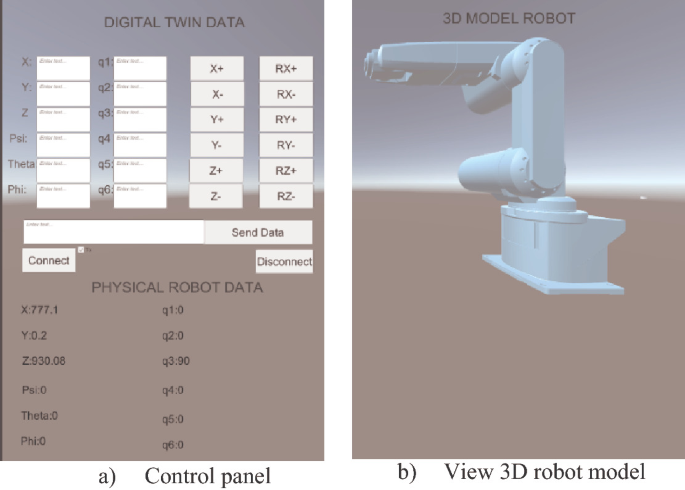
Design of user interfaces


To control the robot, the inverse kinematic model of the robot is formulated, which uses the position (X, Y, Z) and the rotation (RX, RY, RX) of end-effector to calculate joint angles of the physical robot.
An important aspect when building a digital model is the connection between virtual and real environment. In this paper, the connection method based on the RS232 communication is selected which exchanges data between the physical robot and the virtual space. The information is exchanged in both-ways that include joint angles and actual robot status signals.
3 Inverse Kinematic Modelling of the Robot
The inverse kinematic modeling of a robot plays an important role in calculating the values of the joint variables (q1, q2, q3, q4, q5, q6) for control the physical robot in connection with a Digital Twin [10,11,12,13,14]. In this section, we present a analytical solution to the inverse kinematic problem of the robot Mitsubishi RV-12SD. Figure 4 show the feasible workspace of the robot, and Fig. 5 shows the kinematic diagram of the robot mechanism.

The workspace of robot RV-12SD

Kinematic diagram of robot RV-12SD
Note that the Denavit-Hatenberg method is used to define all the link frames as usual. With the kinematic parameters listed in Table 1, the transformation matrices and calculated as follows.
In Eq. (4),
With a desired posture of Robot arm, the end effector position could be defined via \(x_{E}^{{}} ,y_{E}^{{}} ,z_{E}^{{}}\) and orientation is ψ, θ, φ. From that, rotation matrix \({\mathbf{R}}_{E} = {\mathbf{R}}_{6}^{0}\) can be written to find q1, q2 and q3.
It is clearly seen that the values of the three joint q4, q5, q6 do not affect the center wrist (O5) position. On one hand, O5 position in coordinate O6 X6 Y6 Z6 is 0, 0, –d6, so the position of the wrist center can be calculated from the position of end effector (\(x_{E}^{{}} ,y_{E}^{{}} ,z_{E}^{{}}\)) as
The position of O5 on X0Y0 plane is described as shown in Fig. 6.

Projection of O5 on plane X0Y0
In this manner, q1 can be calculated as
On the plane of Link1 and Link2, the joint q1 and q2 are involved as shown in Fig. 7.

Projection on the plane of Link2 and Link3
As seen in Fig. 7, q2 and q3 can be easily calculated. Note that \(l = \sqrt {x_{w}^{2} + y_{w}^{2} } - a_{1}\); \(h = z_{w} - d_{1}\); \(k = \sqrt {a_{3}^{2} + d_{4}^{2} }\); \(b = \sqrt {l_{{}}^{2} + h_{{}}^{2} }\).
In order to calculate q4, q5 and q6, the rotation matrix \({\mathbf{R}}_{3}^{0}\) and \({\mathbf{R}}_{6}^{3}\) must be calculated.
On the other hand,
Hence
Note that \(R_{6}^{3} = R_{A}\), hence we have
Finally, the values of all the joint variables q1, q2, q3, q4, q5 and q6 are analytically calculated with Eqs. (7, 10, 13, 19, 20, 21).
4 Connection of Both the Twins and Control the Robot

Data flow for the communication between the robot and the digital twin model.
To transfer the kinematic data from a control computer to RV-12SD robot controller, command blocks containing a frame of characters are sent to the robot controller through a RS232 port. This protocol makes it easy for constructing a data flow throughout the software and hardware to enable the twin models (3D digital on computer and physical robot). In this digital-physical system, the kinematic data will be stored and used for other control and monitoring purposes when both the twins operate together in real time (Fig. 8).

Testing digital twin model
Figure 9 shows the integration of both the designed digital twin and the physical twin (the robot). After several testing scenarios, it has shown that both the models can collaborate well. By using the control panel with the digital twin model, it is able to control real robot from a virtual environment. Note that by using buttons (X+, X–, Y+, Z+, Z–, RX+, RX–, RY+, RZ+, RZ–) with the added window containing a camera signal of the real robot behavior, the real robot movement interacted with the digital twin simulation can be monitored effectively.
5 Conclusion
In this paper, a case study about design and implementation of a digital twin for control and monitoring a real industrial robot was presented. The 3D digital twin is designed in Unity 3D software, which provides advantages for the collaboration and the real time data connection between the physical-digital models. The inverse kinematics of the real robot is studied and an analytical inverse kinematic solution is yielded, which makes it more effectively and precisely for the control of the robot in cooperation with the digital twin. The implementation and testing results shows that controlling and monitoring a real robot with the support of a collaborating digital twin model is feasible and applicable. This method makes it possible to improve the smartness of a robotic system by using the advancement of the recent development of ICT technology. Using this physical-digital twins for offline programming, testing-simulation, control and monitoring when a robot is required to weld a complex path of high curvature is the future work of this study.
References
Madni, A.M., Madni, C.C., Lucero, S.D.: Leveraging digital twin technology in model-based systems engineering. Systems 7(1), 7 (2019)
Booyse, W., Wilke, D.N., Heyns, S.: Deep digital twins for detection, diagnostics and prognostics. Mech. Syst. Signal Process. 140, 106612 (2020)
Cai, Y., Starly, B., Cohen, P., Lee, Y.S.: Sensor data and information fusion to construct digital-twins virtual machine tools for cyber-physical manufacturing. Procedia Manuf. 10, 1031–1042 (2017)
Cronrath, C., Aderiani, A.R. and Lennartson, B.: Enhancing digital twins through reinforcement learning. In: 2019 IEEE 15th International Conference on Automation Science and Engineering (CASE), pp. 293–298. IEEE (August 2019)
Dröder, K., Bobka, P., Germann, T., Gabriel, F., Dietrich, F.: A machine learning-enhanced digital twin approach for human-robot-collaboration. Procedia Cirp 76, 187–192 (2018)
Ganguli, R., Adhikari, S.: The digital twin of discrete dynamic systems: initial approaches and future challenges. Appl. Math. Model. 77, 1110–1128 (2020)
Guivarch, D., Mermoz, E., Marino, Y., Sartor, M.: Creation of helicopter dynamic systems digital twin using multibody simulations. CIRP Ann. 68(1), 133–136 (2019)
He, R., Chen, G., Dong, C., Sun, S., Shen, X.: Data-driven digital twin technology for optimized control in process systems. ISA Trans. 95, 221–234 (2019)
Liu, J., Zhou, H., Tian, G., Liu, X., Jing, X.: Digital twin-based process reuse and evaluation approach for smart process planning. Int. J. Adv. Manuf. Technol. 100(5–8), 1619–1634 (2018). https://doi.org/10.1007/s00170-018-2748-5
My, C.A., et al.: Mechanical design and dynamics modelling of RoPC robot. In: Proceedings of International Symposium on Robotics and Mechatronics, Hanoi, Vietnam, pp. 92–96 (September 2009)
My, C.A.: Inverse dynamic of a N-links manipulator mounted on a wheeled mobile robot. In: 2013 International Conference on Control, Automation and Information Sciences (ICCAIS), pp. 164–170. IEEE (2013, November)
Chu, A.M., et al.: A novel mathematical approach for finite element formulation of flexible robot dynamics. Mech. Based Des. Struct. Mach. 1–21 (2020)
My, C.A., Makhanov, S.S., Van, N.A., Duc, V.M.: Modeling and computation of real-time applied torques and non-holonomic constraint forces/moment, and optimal design of wheels for an autonomous security robot tracking a moving target. Math. Comput. Simul. 170, 300–315 (2020)
Toai, T.T., Chu, D.-H., My, C.A.: Development of a new 6 DOFs welding robotic system for a specialized application. In: Balas, V.E., Solanki, V.K., Kumar, R. (eds.) Further Advances in Internet of Things in Biomedical and Cyber Physical Systems. ISRL, vol. 193, pp. 135–150. Springer, Cham (2021). https://doi.org/10.1007/978-3-030-57835-0_11
Acknowledgement
This research is funded by Vietnam National Foundation for Science and Technology Development (NAFOSTED) under grant number 107.01-2020.15.
Author information
Authors and Affiliations
Corresponding author
Editor information
Editors and Affiliations
Rights and permissions
Copyright information
© 2022 The Author(s), under exclusive license to Springer Nature Switzerland AG
About this paper

Cite this paper
Vu, M.D., Nguyen, T.N., My, C.A. (2022). Design and Implementation of a Digital Twin to Control the Industrial Robot Mitsubishi RV-12SD. In: Khang, N.V., Hoang, N.Q., Ceccarelli, M. (eds) Advances in Asian Mechanism and Machine Science. ASIAN MMS 2021. Mechanisms and Machine Science, vol 113. Springer, Cham. https://doi.org/10.1007/978-3-030-91892-7_40
Download citation
DOI: https://doi.org/10.1007/978-3-030-91892-7_40
Published:
Publisher Name: Springer, Cham
Print ISBN: 978-3-030-91891-0
Online ISBN: 978-3-030-91892-7
eBook Packages: EngineeringEngineering (R0)