
Abstract
Monetary responses to financial stress have recently become an important issue in macroeconomic and policy discussions in the USA as well as in the EU. In this paper, the authors study two regimes of monetary responses. While the fundamentals of an economy are assumed to have a long-run equilibrium, the adjustment process towards the equilibrium can be different in different regimes. During a period of deteriorated economic conditions, rate cuts are the most often applied policy responses. Therefore, rate cuts can be used as a natural regime identifier. We observe that the financial stress shocks have a large and persistent negative impact on the real side of the economy, and their impact is stronger in the non-rate-cut regime than in the rate-cut regime. A macro-foundation of such a Finance-Macro model type is given in Mittnik and Semmler (J Econ Behav Organ 83:502–522, 2013) and Chen and Semmler (J Econ Dyn Control 91:318–348, 2018). The agents can, in a finite horizon context, borrow and accumulate assets where however the above two scenarios may occur. The model is solved through nonlinear model predictive control (NMPC). Empirically we use a multi-regime cointegrated VAR (MRCIVAR) to study the impact of financial stress shocks and monetary policy on the macroeconomy in different countries.
Access provided by Autonomous University of Puebla. Download chapter PDF
Keywords
- Multi-regime cointegrated VAR (MRCIVAR)
- Cycles
- Nonlinear model predictive control (NMPC)
- Business cycles
1 Introduction
Since the seminal papers on cointegration by Engle and Granger [7] and Johansen [16] vector error correction model (VECM) has been widely used to model macroeconomic time series. The virtue of VECM is that it permits to test both the economic concepts of equilibrium and the adjustment process towards the equilibrium. Then, the long-run equilibrium relations as well the adjustment to the equilibrium can be empirically testable. However, the phenomena of business cycles point to differences in the adjustment process during different phases of the business cycle. Hence, regime switching vector autoregressive models have been used by many researchers, such as Hamilton [11], Mittnik et al. [18] and Chen et al. [5], to take into account the impact of the different phases in the business cycle. Balke et al. [3] combine these two classes of models and present the regime switching vector error correction models. Since then, regime switching VECM has been applied in numerous empirical analysis.
Balke et al. [3] applied threshold VECM to reflect discrete adjustment responses to a cointegrating relationship when it is “too far from the equilibrium”. The cointegration relation is obtained through a regression relying on the super consistency of the least square (LS) estimator. The model specification is verified through tests of the existence of the threshold nonlinearity. Hansen et al. [12] propose a maximum likelihood estimation for a two regime threshold VECM, where the switching variable is also the endogenous cointegrating relationship. A grid search algorithm is proposed to estimate both the cointegration vector and the threshold value for the regime classification simultaneously. An R package is available for this class of threshold VECMs.Footnote 1
Most empirical research works of threshold VECMs follow the approach proposed in Hansen et al. [12], Bec et al. [4], Saikkonen [20, 21]. They present a more general class of regime switching error correction models, where the number of regimes can be more than two and the switching can be a discontinuous adjustment or a continuous smooth transition. Saikkonen [21] points out a difficulty in this class of models is “to determine theoretically the exact number of I(1) components in the models”. Hence, it is inconclusive how to test the cointegration rank in this class of models. Common to the mentioned regime switching error correction models is that the cointegrating relations are linear, and the adjustments are nonlinear or switching. The thresholds are determined endogenously.
Gonzalo et al. [9] take a different approach to regime switching error correction models. In their models, the cointegrating relations are switching whereas the adjustment is linear. The switching variable is an exogenously stationary variable. This approach is less attractive as the switching long-run equilibrium relations are hard to justify. In addition, leaving an influencing variable not included in the VECM is also hard to justify. In this chapter, we will present a specific regime switching VECM where the cointegrating relation is linear, while the switching is determined by a stationary variable in the system.
2 Self-exciting Threshold Cointegrated Autoregressive Model
We consider a regime switching autoregressive model of order p that consists of two regimes:

where X t is a p dimensional vector, β is a p × r matrix with p > r, β is called cointegration vectors, r is called cointegration rank, f t−d is the threshold variable observed at time t − d, and the regimes are defined by the prespecified threshold values −∞ = τ 0 < τ < ∞. For f t−d = g(ΔX j,t−1, ΔX j,t−2, …, ΔX j,t−d), i.e., the threshold variable is a function of the lagged endogenous variables
i.e., the threshold variable is simply a component of X t with one lag. τ is the threshold value. The model is called self-exciting threshold cointegrated autoregressive model of order L with two regimes, and it is denoted as SETCIAR(L, d, 2).
Our model differs from many threshold VECMs mentioned in the previous section in that the switching variable is an I(0) (integrated of order 0) variable which does not involve any estimation. In addition, the threshold value τ is such that the sample can be separated into two different regimes by a suitable setting.
This setting simplifies many technical issues in parameter estimation and specification tests. In principle, the data analysis could be conducted in the two separate subsamples, each of which is a conventional VECM. The only issue of concern is how to take into account the restriction of the same cointegration relations across the two regimes to increase the efficiency of estimation.
2.1 Test of Cointegration Rank
As described in the last section, the test of the cointegration rank could be done in principle in two separate subsamples. This approach might, however, lead to conflicting results with respect to the cointegration rank in the two subsamples. We use the fact that the cointegration space is identical in the two regimes and test the cointegration rank in the whole sample. The procedure can be described as follows:
-
Run the auxiliary regression:
$$\displaystyle \begin{aligned} \varDelta X_t = \hat{\pi}_0 + \sum_{i=1}^{L-1}\hat{\pi}^{(1)}_l\varDelta X_{t-l}{\mathbf{1}}_{[X_{j,t-1} \le \tau]} + \sum_{i=1}^{L-1}\hat{\pi}^{(2)}_l\varDelta X_{t-l}{\mathbf{1}}_{[X_{j,t-1} > \tau]} + \hat{u}_t \, , \end{aligned} $$(20.2)$$\displaystyle \begin{aligned} X_{t-1} = \hat{\theta}_0 + \sum_{i=1}^{L-1}\hat{\theta}^{(1)}_l\varDelta X_{t-l}\mathbf{ 1}_{[X_{j,t-1} \le \tau]} + \sum_{i=1}^{L-1}\hat{\theta}^{(2)}_l\varDelta X_{t-l}\mathbf{ 1}_{[X_{j,t-1} > \tau]} + \hat{v}_t \, , \end{aligned} $$(20.3) -
let
$$\displaystyle \begin{aligned}\hat{\varSigma}_{vv}=\frac{1}{T}\sum^{T}_{t=1}\hat{v}_t\hat{v}^{\prime}_t \, ,\end{aligned}$$$$\displaystyle \begin{aligned}\hat{\varSigma}_{uu}=\frac{1}{T}\sum^{T}_{t=1}\hat{u}_t\hat{u}^{\prime}_t \, ,\end{aligned}$$$$\displaystyle \begin{aligned}\hat{\varSigma}_{vu}=\frac{1}{T}\sum^{T}_{t=1}\hat{v}_t\hat{u}^{\prime}_t \, ,\end{aligned}$$$$\displaystyle \begin{aligned}\hat{\varSigma}_{uv}=\frac{1}{T}\sum^{T}_{t=1}\hat{u}_t\hat{v}^{\prime}_t \, .\end{aligned}$$ -
Calculate the eigenvalues of
$$\displaystyle \begin{aligned} \hat{\varSigma}_{vv}^{-1}\hat{\varSigma}_{vu}\hat{\varSigma}_{uu}^{-1}\hat{\varSigma}_{uv}, \end{aligned} $$(20.4)with ordered eigenvalues \(\hat {\lambda }_1>\hat {\lambda }_2>\ldots >\hat {\lambda }_p\). These eigenvalues can be used to calculate the Johansen test statistics. Following [15], we have the trace test:
$$\displaystyle \begin{aligned} \mathcal{L}_A - \mathcal{L}_0 = -T \sum^p_{i=r+1}\log(1-\lambda_i). \end{aligned} $$(20.5)The critical value for the tests can be found in [17].
2.2 Parameter Estimation
Following Lemma 13.1 in [17], after a proper normalization, the eigenvectors of (20.4) that correspond the r largest eigenvalues span the cointegration space and hence are consistent estimator of β. After obtaining a consistent estimator of \(\hat {\beta }\), the other regime-dependent parameters can be estimated through the following regression:
In the above regression we plug in the estimated \(\hat {\beta }X_{t-1}\) as a regressor. Because \(\hat {\beta }\) is consistent, then the estimator \(\hat {\alpha }^{(i)}\), \(\hat {\phi }^{(i)}_l\) are consistent for i = 1, 2 and l = 1, 2, …, L − 1.
2.3 Test of Switching
A key hypothesis of the regime switching VECM in (20.1) is the existence of two regimes. This should, however, be tested against the data. To test the null of no switching against the alternative of switching, a likelihood ratio test can be applied, given that the cointegrating relations have consistently been estimated. This boils down to testing the following parameter restrictions in the linear regression of (20.6):

3 Test of the Model on Economic Data
The dynamic interaction between financial stress and real output has drawn renewed attention of many researchers after the global financial crisis. Mittnik et al. [18, 19] develop a decision theoretical model that results in asymmetric interaction in different regimes. Mittnik et al. [18] and Chen et al. [5] apply regime switching VAR models to take into account the nonlinearity in the data. Following this approach, we apply a regime switching vector error correction model to investigate asymmetric adjustments to the equilibrium in different regimes.
We consider three variables in our study: the IMF financial stress index, the industrial output index, and the short-term interest rate. These three variables are chosen to be a measure of the real output, a measure of the financial stress, and a measure of the policy responses, respectively. The data are from IMF and OECD statistics.
The IMF Financial Soundness Indicators (FSI) is available for a large number of EU countries [1]. Footnote 2 The IMF’s (2011) FSI Footnote 3 refers to three major sources and measures of instability, namely: (1) a bank related index—a 12-month rolling beta of bank stock index and a Ted or interbank spread, (2) a security related index—a corporate bond yield spread, an inverted term spread, and a monthly stock returns (measured as declines), 6-month rolling monthly squared stock returns and finally, (3) an exchange rate index—a 6-month rolling monthly squared change in real exchange rates. All three sets of variables are detrended and scaled with their standard deviations in order to normalize the measures. Both the Industrial Production Indices and the short run interest rates are taken from the OECD Statistics.
3.1 Discrimination of Regimes
Identification of regimes is critical in modelling a Multi-Regime VAR (MRVAR) model [8, 19]. While many researches identify the regimes based on the sign and the size of the error correction term, which represent deviations from the long-run equilibrium, we identify the regime by the periods of the interest rate cuts or the periods of interest rate hikes. Typically during recession periods of a business cycle, we observe consecutive interest rates cuts, while during expansion periods, we observe rate hikes. Interest rate cuts and interest rate hikes reflect different policy responses to different economic circumstances, which aim at adjusting the economy to the long-run equilibrium state. This way of identification of the regimes simplifies the model specification and inference. In principle, we could divide the cointegration analysis in two separate subsamples of the respective regimes. However, a joint analysis will increase the efficiency of the inference and also avoid the problem that we might obtain two different sets of cointegration relations.
3.2 Model Specification
The specification of the model consists of the following three steps:
-
Test of unit roots in the time series
Country
USA
DEU
FRA
ITA
ESP
\(\log (IP)\)
ADF
0.0100
0.02396
0.2013
0.1491
0.4520
PP
0.5449
0.1041
0.4711
0.4966
0.7575
CFSI
ADF
0.7328
0.6946
0.3821
0.2185
0.2185
PP
0.9481
0.8363
0.8438
0.841
0.8410
R
ADF
0.4813
0.0907
0.1197
0.0427
0.0972
PP
0.8503
0.5502
0.5597
0.4685
0.4166
-
Selection of the lag length in a two regime VAR in level L, for a system consisting of three variables \(y_t=(\log (IP_t),CFSI_t,R_t)'\).
The results of the lag selection using the BIC criteria are summarized in the following table:
Country
USA
DEU
FRA
ITA
ESP
Lag length regime 1
2
2
2
2
2
Lag length regime 2
2
2
2
2
2
-
Testing the cointegration rank in a two regime VECM for the selected lag length L − 1. The following tables show the results of Johansen trace test for the five countries respectively:
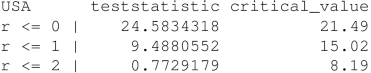


The test results show that only in the system of FRA there are two cointegration relations, while in all other four countries there is only one cointegration relation in the system respectively.
-
Model selection based on information criteria to discriminate between one regime VECM and two regime VECM. We estimate a standard one regime VECM and a two regime VECM for a system consisting of three variables y t = (FSI t, IP t, R t)′. We use AIC to discriminate between a VECM or an MRVECM. The AIC is given by
$$\displaystyle \begin{aligned} AIC(M,p_1,p_2) = \sum_{j=1}^M\left[T_j \log|\hat{\varSigma}_j|+2n\left(np_j+\frac{n+3}{2}\right) \right], \end{aligned} $$(20.7)where M = 2 is the number of regimes; p j is the autoregressive order of regime j; T j is the number of observations associated with regime j; \(\hat {\varSigma }_j\) is the estimated covariance matrix of the residuals of regime j; and n denotes the number of variables in the vector y t.Footnote 4
Country
USA
DEU
FRA
ITA
ESP
AIC OR
198.6
358.8
100.3
299.2
212.5
AIC MR
34.6
327.6
73.7
238.6
180.7
The values of the AIC criteria of the one regime models are all larger than those of the AIC criteria of the two regime models. Hence the AIC information criteria favour the two regime VECMs.
-
Test of regime switching
Since a one regime VACM can be seen as a multi-regime with identical parameters in the different regimes, we can test the existence of multi-regimes through testing the null of equal parameters across different regimes against the alternative of unequal parameters in different regimes.
$$\displaystyle \begin{aligned} H_O: (\alpha^{(1)}, \phi^{(1)}_l,\ldots,\phi^{(1)}_{L-1}) = (\alpha^{(2)},\phi^{(2)}_l,\ldots\phi^{(2)}_{L-1}) \end{aligned}$$$$\displaystyle \begin{aligned} H_A: (\alpha^{(1)}, \phi^{(1)}_l,\ldots,\phi^{(1)}_{L-1}) \neq (\alpha^{(2)},\phi^{(2)}_l,\ldots\phi^{(2)}_{L-1}) \end{aligned} $$Country
USA
DEU
FRA
ITA
ESP
p-value
1.005E−13
0.00010
6.47E−08
6.84E−10
9.98E−06
The test results show clearly that the null of one regime is rejected in all five countries, i.e., the data support the specification of regime switching VECMs. This is consistent with the results of model selection based on the AIC criteria.


3.3 Impulse and Response
The following impulse response functions (see Fig. 20.1) are the within-regime impulse response function (see Ehrmann [6] for more details). They can be used to trace out short run dynamics of the system. The impulses are all a one unit impulses, the responses are the responses of the system in (20.1), i.e., they are the industrial output, the financial stress index and the short run interest rate denoted by (IP t, FSI t, R t), respectively.


Impulse response function of the rate-cutting and the non-rate-cutting regimes USA showing that: (1) a positive output shock may have positive effect on the output, almost no effect on FSI and R in the rate-cut regime, and a negative effect in the non-rate-cut regime on financial stress short-term interest rate; (2) a positive financial stress shock has positive effects on the financial stress in non-rate-cut and rate-cut regimes, negative effects on the output in both regimes, opposite effects on the short-term interest rate; (3) a positive interest rate shock has positive effects on the short-term interest rate, a negative impact on the output in the non-rate-cut regime, a positive impact in the rate-cut regime, a positive effect on the financial stress in the non-rate-cut regime, and negligible in the rate-cut regime
The three graphs on the first row are responses of (IP t, FSI t, R t) to a one unit positive impulse of IP. The graphs on the second row are responses to the shock of a one unit increase in FSI. The graphs in the third row are responses to the shock of a one unit increase in R. The first three rows are impulse responses in the rate-cut regime. The second three rows are impulse responses in the non-rate-cut regime. We observe:
-
A one unit output shock will have a long lasting positive effect on the output over 20 periods. The effects are stronger in the non-rate-cut regime than in the rate-cut regime. In the rate-cut regime the effects of the output shock on FSI and R are statistically insignificant, in the non-rate-cut regime the output shock will decrease the financial stress and decrease the short-term interest rate.
-
A one unit financial stress shock has lasting effects on the financial stress in both regimes over 20 quarters. Its effects are more persistent in the non-rate-cut regime than in the rate-cut regime. The shock has negative effects on the output in both regimes. Interestingly, the shock has opposite effects on the short-term interest rate. While in the rate-cut regime the financial stress shock will decrease the short-term rate, in the non-rate-cut regime it will increase the short-term interest rate.
-
The one unit interest rate shock has lasting effects on the short-term interest rate. Its effects are significantly larger in the non-rate-cute regime than in the rate-cut regime. The interest rate shock has different effects in the two regimes. While in the non-rate-cut regime an interest hike shock has a negative impact on the output, it has a positive impact on the output in the rate-cut regime, though the effects are not statistically significant. In the non-rate-cut regime, the interest rate shock will increase the financial stress; its effect in the rate-cut regime is insignificant.
The following graphs (see Fig. 20.2) are the impulse response functions of Germany. The three graphs on the first row are responses of (IP, FSI, R) to a one unit impulse of IP. The three graphs in the second row are responses to FSI. The first three rows contain the responses in the rate-cut regime and the second three rows contain the responses in the non-rate-cut regime.


Impulse response function of the rate-cutting and non-rate-cut regimes in DEU showing that: (1) A positive output shock may have positive effect on the output, almost no effect on FSI and R in the rate-cut regime, and a negative effect in the non-rate-cut regime on financial stress short-term interest rate; (2) A positive financial stress shock has positive effects on the financial stress in non-rate-cut and rate-cut regimes, negative effects on the output in both regimes, opposite effects on the short-term interest rate; (3) A positive interest rate shock has positive effects on the short-term interest rate, a negative impact on the output in both regimes, a positive (but statistically insignificant) effect on the financial stress in the non-rate-cut regime and rate-cut regime
-
A one unit output shock will have a long lasting positive effect on the output over 20 periods. The effects are similar and statistically significant in both the non-rate-cut regime and the rate-cut regime. The one unit output shock has no statistically significant effect on the financial stress and the short-term interest rate in both regimes.
-
The shock of a one unit increase in financial stress index has lasting effects on the financial stress in both regimes. While in the rate-cut regime the effects die out after 20 periods, the effects remain significant in the non-rate-cut regime. The shock has negative effects on the output in both regimes. However, the effects in the non-rate-cut regime are stronger than in the rate-cut regime. The shock has a negative effect on the short-term interest rate in the rate-cut regime, while its effects in the non-rate-cute regime are statistically insignificant.
-
A one unit interest rate shock has lasting effects on the short-term interest rate in the non-rate-cut regime. Its effects in the rate-cute regime vanish after 10 periods. The unitary shock (one unit positive impulse) in interest rate has a negative effect on the output in both regimes, though the effects are not statistically significant. In both regimes, the shock of one unit increase in the short-term interest rate will increase the financial stress, although these effects are not statistically significant.
The next diagrams are the impulse response functions for Italy (see Fig. 20.3). The orders of the IRFs are organized in the same way as in the previous graphs. In the Italian case we observe:
-
A one unit output shock will have a lasting effect on the output in both regimes. The effect is slightly stronger in the non-rate-cut regime. Its effects on the financial stress and the short-term interest rate are statistically insignificant in both regimes.
Fig. 20.3 

Impulse response function of the rate-cutting and the non-rate-cutting regimes ITA showing that: (1) A positive output shock may have positive effect on the output and no statistically significant effect on FSI and R; (2) A positive financial stress shock has positive effects on the financial stress in non-rate-cut and rate-cut regimes, negative effects on the output in both regimes, opposite effects (but statistically not significant) on the short-term interest rate; (3) A positive interest rate shock has positive effects on the short-term interest rate, a positive impact on the output in both regimes and no effect on the financial stress
-
A one unit financial stress shock has a significant negative impact on output in both regimes. The effects are stronger in the non-rate-cut regime. The effects of the financial stress shock on financial stress die out in the rate-cut regime after 15 periods, while the effects remain persistent in the non-rate-cut regime. Notably, the responses of the short-term interest rate are negative in the rate-cut regime, but positive in the non-rate-cut regime, though the effects are not statistically significant.
-
While a one unit interest rate shock has no significant effects on the financial stress in both regimes, it has positive impact on output in both regimes. The shock has positive and persistent effects on the short-term interest rate in both regimes. The effects are stronger in the rate-cut regime.


Because the impulse response functions of the four European countries are by and large very similar (see Figs. 20.2, 20.3, 20.4 and 20.5), we summarize the features of the IRFs in the following Table 20.1.
-
While the responses of IP to FSI are negative and significant in both regimes, the responses of IP to R are in most cases statistically insignificant in both regimes. The responses of IP to an output shock are statistically significant and long lasting in both regimes.
Fig. 20.4 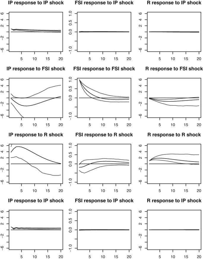

Impulse response function of the rate-cutting and the non-rate-cutting regimes FRA displaying similar results of Fig. 20.3
Fig. 20.5 

Impulse response function of the rate-cutting and the non-rate-cutting regimes ESP displaying similar results of Fig. 20.3
Table 20.1 Summary of the results of the impulse response functions for Germany, France, Italy and Spain -
The responses of FSI to financial stress shocks are decreasingly lasting in both regimes. However, while the responses will die out in the rate-cut regime, the responses remain positive in the non-rate-cut regime permanently. The responses of FSI to interest rate shocks and to output shocks are statistically insignificant in both regimes.
-
The responses of R to output shocks are statistically insignificant in both regimes. Notably, the responses of R to a financial stress shock are negative and significant in the rate-cut regime, while the responses are positive and significant in the non-rate-cut regime. The responses of R to short-term interest rate shocks are in most cases persistently lasting in both regimes.


4 Concluding Remarks
Using the IMF financial stress index and OECD industrial production index and short-term interest rate data, for the USA, the EU countries, our regime switching vector error correction model enables us to conduct a parallel analysis in different regimes. By using the regime switching VECM, we could show that the responses are asymmetric in the two different regimes, namely the rate-cut regime and the non-rate-cut regime.
Generally, the financial stress shocks have a large and persistent negative impact on the real side of the economy, and the impact is stronger in the non-rate-cut regime than in the rate-cut regime. This asymmetric impact of financial stress on the real side of the economy is because rate cuts as an instrument of the monetary policy are often aimed at reducing the financial stress and hence offset the impact of the latter on the real activity, while in the rate hikes regime increase in interest rate will worsen the financial stress, enforcing the adverse effect of the latter on the real activities.
Looking at the impact of real activities on the financial stress: they are statistically insignificant in both regimes. Empirically, we find that financial stress shocks have asymmetric effects on the short-term interest rate, depending on the regime the economy is in. Overall, in the rate-cut regime a financial stress shock will decrease the short-term rate while in the non-rate-cut regime the shock will increase the short-term rate though in some cases the effects are not statistically significant.
While there is heterogeneity across countries with smaller countries showing weaker channels in the financial-real interaction, there is more similarity in larger economies. Across countries, there are common features in the sense that the European countries show very similar response patterns in the two regimes, respectively.
Notes
- 1.
See Stigler et al. [22] for more details.
- 2.
The Federal Reserve Bank of Kansas City and the Fed St. Louis have also developed a general financial stress index, called KCFSI and STLFSI, respectively. The KCFSI and the STLFSI take into account the various factors generating financial stress. The KC index is a monthly index, the STL index a weekly index, to capture more short run movements, see also Hatzius et al. [13]. Those factors can be taken as substitutes for the leverage ratios as measuring financial stress. See also the Bank of Canada index for Canada, i.e., Illing and Lui [14]. Both the KCFSI and STLFSI include a number of variables and financial stress is related to an: (1) increase in the uncertainty of the fundamental value of the assets, often resulting in higher volatility of the asset prices, (2) increase in uncertainty about the behaviour of the other investors, (3) increase in the asymmetry of information, (4) increase in the flight to quality, (5) decrease in the willingness to hold risky assets, and (6) decrease in the willingness to hold illiquid assets. The principle component analysis is then used to obtain the FSI. Linear OLS coefficients are normalized through their standard deviations and their relative weights computed to explain an FSI index. A similar procedure is used by Adrian and Shin [2] to compute a macro economic risk premium. We want to note that most of the variables used are highly correlated with credit spreads. The latter have usually the highest weight in the index, for details see Hakkio and Keeton [10, Tables 2–3].
- 3.
This is published for advanced as well for developing countries, see IMF (2008) and IMF FSI (2011).
- 4.
The AIC takes into account for possible heterogeneity in the constant terms, c j, and residual covariance, Σ j, across regimes. This AIC criterion is also applied in Mittnick and Semmler [18].
References
The IMF 2019 Financial Soundness Indicators Compilation Guide (2019 FSI Guide) (2020). https://www.imf.org/en/Data/Statistics/fsi-guide. Accessed 20 Oct 2020
Adrian, T., Shin, H.S.: Liquidity and leverage. J. Finan. Intermed. 19(3), 418–437 (2010)
Balke, N.S., Fomby, T.B.: Threshold cointegration. Int. Econ. Rev. 3, 627–645 (1997)
Bec, F., Rahbek, A.: Vector equilibrium correction models with non-linear discontinuous adjustments. Econ. J. 7(2), 628–651 (2004)
Chen, P., Semmler, W.: Financial stress, regime switching and spillover effects: evidence from a multi-regime global VAR model. J. Econ. Dyn. Control 91, 318–348 (2018)
Ehrmann, M., Ellison, M., Valla, N.: Regime-dependent impulse response functions in a markov-switching vector autoregression model. Econ. Lett. 78(3), 295–299 (2003)
Engle, R.F., Granger, C.W.: Co-integration and error correction: representation, estimation, and testing. Econometrica 55, 251–276 (1987)
Ernst, E., Semmler, W., Haider, A.: Debt-deflation, financial market stress and regime change–evidence from Europe using MRVAR. J. Econ. Dyn. Control 81, 115–139 (2017)
Gonzalo, J., Pitarakis, J.Y.: Threshold effects in cointegrating relationships. Oxf. Bull. Econ. Stat. 68, 813–833 (2006)
Hakkio, C.S., Keeton, W.R. et al.: Financial stress: what is it, how can it be measured, and why does it matter? Econ. Rev. 94(2), 5–50 (2009)
Hamilton, J.D.: Time Series Analysis. Princeton University Press, Princeton (2020)
Hansen, B.E., Seo, B.: Testing for two-regime threshold cointegration in vector error-correction models. J. Econ. 110(2), 293–318 (2002)
Hatzius, J., Hooper, P., Mishkin, F.S., Schoenholtz, K.L., Watson, M.W.: Financial conditions indexes: A fresh look after the financial crisis. Tech. rep., National Bureau of Economic Research (2010)
Illing, M., Liu, Y.: Measuring financial stress in a developed country: an application to Canada. J. Financ. Stab. 2(3), 243–265 (2006)
Johansen, S.: Statistical analysis of cointegration vectors. J. Econ. Dyn. Control 12(2–3), 231–254 (1988)
Johansen, S.: Estimation and hypothesis testing of cointegration vectors in Gaussian vector autoregressive models. Econometrica 59, 1551–1580 (1991)
Johansen, S.: Likelihood-Based Inference in Cointegrated Vector Autoregressive Models. Oxford University Press, Oxford (1995)
Mittnik, S., Semmler, W.: Regime dependence of the fiscal multiplier. J. Econ. Behav. Organ. 83, 502–522 (2013)
Mittnik, S., Semmler, W.: Estimating a banking-macro model using a multi-regime VAR. In: Advances in Non-linear Economic Modeling, pp. 3–40. Springer, Berlin (2014)
Saikkonen, P.: Stability results for nonlinear error correction models. J. Econ. 127(1), 69–81 (2005)
Saikkonen, P.: Stability of regime switching error correction models under linear cointegration. In: Econometric Theory, pp. 294–318 (2008)
Stigler, M.: Threshold cointegration: overview and implementation in R (2010). http://stat.ethz.ch/CRAN/web/packages/tsDyn/vignettes/ThCointOverview.pdf. Accessed 19 Jul 2020
Author information
Authors and Affiliations
Corresponding author
Editor information
Editors and Affiliations
Rights and permissions
Copyright information
© 2021 The Author(s), under exclusive license to Springer Nature Switzerland AG
About this chapter

Cite this chapter
Chen, P., Semmler, W. (2021). Financial Stress, Regime Switching and Macrodynamics. In: Orlando, G., Pisarchik, A.N., Stoop, R. (eds) Nonlinearities in Economics. Dynamic Modeling and Econometrics in Economics and Finance, vol 29. Springer, Cham. https://doi.org/10.1007/978-3-030-70982-2_20
Download citation
DOI: https://doi.org/10.1007/978-3-030-70982-2_20
Published:
Publisher Name: Springer, Cham
Print ISBN: 978-3-030-70981-5
Online ISBN: 978-3-030-70982-2
eBook Packages: Economics and FinanceEconomics and Finance (R0)