Model-Based Machine Learning and Approximate Inference

Abstract

In this chapter, we introduce the building blocks of Model-Based Machine Learning (MBML). We explain what it is and discuss its main enabling techniques: Bayesian inference, graphical models, and, more recently, probabilistic programming. Frequently, models are complex enough so that exact inference is not possible, and one must resort to approximate methods. We broach deterministic distributional approximation methods for approximate inference, focusing on Variational Bayes, Assumed Density Filtering, and Expectation Propagation, going through derivations, advantages, issues, and modern extensions.

By the end of this chapter, the reader should:

• Understand the various advantages of the model-based approach,

• Discern the benefits and issues of Bayesian inference,

• Be capable of understanding and implementing variational Bayes and expectation propagation,

• Understand the mean-field approximation,

• Comprehend the relations between the different variational methods,

• Know the modern landscape of stochastic and black-box inference methods.

3.1 Model-Based Machine Learning

Model-Based Machine Learning (MBML) aims at providing a specific solution for each application. It encodes the set of assumptions for a given application explicitly in the model. Consequently, we are able to create a wide range of highly tailored models under a single development framework.

The clear picture of what is the model decouples the model structure from the learning (inference) algorithm. This segregation allows their independent formulation and the application of the same inference method to different models and vice versa, generating a large number of possible combinations. The unified framework facilitates rapid prototyping and comparison, allowing the derivation of many traditional ML techniques as special cases of certain model-inference configurations (see examples in Sect. 3.1.1).

One might question why do we want to infer probability distributions or even what are the advantages over something simpler such as point estimates, which are single values that already give us answers. The problem in considering only the most likely solution comes from losing information of the underlying variability and robustness of the model. Let us consider a trivial example to illustrate this issue:

Example

An ambulance must take a dying person to the nearest hospital, and there are two possible routes, $\mathcal {A}$ and $\mathcal {B}$. $\mathcal {A}$ takes about 15 min, while $\mathcal {B}$, 17. Which one should the driver choose? Now, the driver further considers that the patient must get to the hospital within 20 min and $\mathcal {A}$ consists of regular urban streets with semaphores and possible traffic jams and that his predicted travel time may vary up to eight minutes, whereas $\mathcal {B}$ is an express lane for medical emergencies and the estimated time varies by no more than one minute. Would the choice still be the same?

The highlighted keywords above give us a sense of the intrinsic variability in our problem, and disregarding that information may be misleading. In the above example, it is clear that the average time is not sufficient information and that the uncertainty is critical for making a more conscious decision. Probability theory provides a principled framework for modeling uncertainty. As seen in our example, probabilistic models allow us to reason and perform decision-making, anticipate the future and plan accordingly, and detect unexpected events, among others; all by learning probability distributions of the data. Not only we can understand almost all ML through probabilistic lenses but also connect it through this perspective to every other computational science [22, p. 2].

3.1.1 Probabilistic Graphical Models

Full joint distributions are generally intractable. Therefore, we resort to structured models [4], which associate probability distributions over only a few variables providing considerable computational simplifications.

One flexible paradigm is Probabilistic Graphical Model (PGM) [12], which use a diagrammatic representation for compactly encoding a complex distribution over a high-dimensional space [12], as depicted in Fig. 3.2, where the most frequent elements are:

• vertices or nodes: denote random variables (also commonly called nodes), which can be shaded if observed or empty otherwise;

• edges: capture the dependency between vertices;

• plates: symbolize that the enclosed subgraph is repeated the number of times indicated by the subscript in the bottom right of the plate, as illustrated in Fig. 3.1.

  Fig. 3.1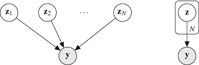

  

  Equivalence of the shorthand plate notation

3.1.1.1 Direct Acyclic Graphs

Let be the set of all vertices of a graph. Define a parent of the vertex i as the vertex whose directed edge points to i. Further define the parent set Π _i as the set of all vertices that are parents of the vertex i.

In the Directed Acyclic Graph (DAG) approach, exemplified in Fig. 3.2a, each vertex together with its parent set Π _i defines a local probability distribution p(x _i | Π _i) over the random variable x _i associated with the corresponding vertex i. The existence of an edge from i to j indicates that i causes j, while the absence indicates that the nodes are independent.

Fig. 3.2

Examples of probabilistic graphical models. In either cases, vertices represent random variables and edges their dependency relation. Bayesian networks (a) encode causation through the edge’s direction, i.e., x ₁ depends on z ₁, z ₂, and z ₃, being their effect. On the other hand, Markov random fields, also known as undirected graphical models, encode symmetrical dependency through the edges, with no cause–effect relation. (a) Bayesian network. (b) Markov random field

The collection of all local probability distributions p(x _i | Π _i) over the random variables x _i describes the joint probability of the model:

(3.1)

This class of models is frequently referred to as Bayesian network, despite no intrinsic need for Bayesian methods. They are so called because they use the Bayes’ rule for defining the probability distributions [23].

3.1.1.2 Undirected Graphs

Contrary to DAGs, undirected graphs, exemplified in Fig. 3.2b, have no cause–effect relation between its nodes and cannot describe a generative process. Instead of describing the full joint distribution in terms of conditionals, undirected graphs factorize the joint distribution over groups of fully connected nodes (maximal cliques), each characterized by a potential function [12]. The potential function of a group is not a valid probability distribution, but the set of all such groups gives the joint distribution according to

(3.2)

where Z is the normalizing constant.

3.1.1.3 The Power of Graphical Models

Many traditional ML and signal processing algorithms can be derived as special cases of graphical models combined with the appropriate inference algorithms. Moreover, many of them can be represented by simple graphical structures and be effortlessly combined [4]. For example:

• 1. Principal Component Analysis (PCA) can be formulated as a generative process with the latent variable z corresponding to the principal component subspace (Fig. 3.3a). Observations y are noisy versions of the linear mapping Wz + μ, where τ is the noise precision, which is the same for all directions. Assuming all distributions to be Gaussian, using MLE for determining W and μ, and taking the limit τ →∞, one obtains the standard PCA model [3, ch. 12].

  Fig. 3.3

  

  Probabilistic graphical models of traditional machine learning algorithms. In the PCA model (a), the principal component subspace is represented by the latent variable z, which cannot be directly observed. We only know the y values that are noisy observations of the true underlying generative $\mathbf {y} = \mathbf {W}\mathbf {z} + \boldsymbol {\mu } + \mathcal {N}(0,\tau )$. In the GMM (b), each of the K modes has its set of unknown defining parameters, i.e., μ and Σ, and is selected by the latent indicator variable Z, whose observation probability is θ

• 2. Gaussian Mixture Model (GMM) (Fig. 3.3b) with K modes is represented by a K-dimensional latent indicator variable z that follows a categorical distribution with probabilities, the mixture weights, given by θ. Each mode has its own mean μ and variance Σ. For other types of mixture, the difference is in the type of parameters that define the K modes, i.e., μ and Σ.

PGMs can be easily customized to a specific application or modified if the requirements of the application change.

3.1.2 Probabilistic Programming

Probabilistic programming is a tool for statistical modeling. It borrows lessons from computer science and common programming languages to construct languages that allow the denotation and evaluation of inference problems [32]. It frees the developer from complex low-level details of probabilistic inference, allowing him or her to concentrate on issues more specific to the problem at hand, such as the model and the choice of inference method. Similarly to high-level programming languages that abstract away architecture-specific implementation details, it boosts system performance and productivity. In Fig. 3.4 we draw a parallel between computer science, statistics, and probabilistic programming.

Fig. 3.4

An intuitive view of probabilistic programming and how it differs from the common computer science paradigm. Shaded boxes indicate the information that is available. Instead of inputting the required parameters to run the program and obtain the desired output, probabilistic programming tries to recover the parameters from the observations generated by the program. This process is similar to inference in statistics

One of the cornerstones for the deep learning success was the development of specialized programming libraries that facilitate model specification and automatize differentiation, relieving the user from the need of manually deriving the gradients for optimization. This genre of software led to the widespread use of deep learning. Nowadays, there is no need to actually understand the basics of neural networks or even differential calculus to try and run a model. Still, it does not mean that whatever the model may be it will be useful or meaningful. Probabilistic programming aims to achieve the same for probabilistic ML [32]. It also allows rapid prototyping and testing of ideas, allowing the field to flourish and pushing industry adoption.

Modern probabilistic programming languages provide a more powerful framework than PGM. Computer programs accept recursion and control flow statements that are otherwise difficult to represent [7]. There is a myriad of different languages, each with its own set of specific features: some are explicitly restrictive, others specialize in a certain type of inference techniques, or yet are general purpose. A non-extensive list includes Pyro [2], Stan [6], WebPPL [8], Infer.NET [21], PyMC3 [28], Edward [30], and BUGS (from 1995) [33].

3.2 Approximate Inference

As briefly alluded in the previous section, it is frequently unfeasible to compute posterior distributions and marginals for many models of practical interest. In the continuous case, there may not be a closed-form analytical solution or it may be just too complex for numerical computation. In the discrete case, summing over all possible configurations, though possible in principle, may not be viable if the total number of combinations grows exponentially.

In such cases we have two options: either to successively simplify the model until exact inference is possible or to perform approximate inference in the original model. On this matter, John Tukey stated [31, p. 13], “Far better an approximate answer to the right question, which is often vague, than an exact answer to the wrong question, which can always be made precise.”

There are two broad classes of approximation schemes: deterministic and stochastic. The latter relies on Monte-Carlo sampling to approximate expectations over a given distribution. Given infinite computational resources, they converge to the exact result, but, in practice, sampling methods can be computationally expensive. On the other hand, deterministic methods consist of analytical approximations to the posterior distribution and, as a consequence, cannot generate exact results. Hence, both methods are complementary.

In this chapter, we discuss variational methods, which are deterministic. We start by its most prominent representative, Variational Inference (VI). Later, we present an alternative variational framework known as Expectation Propagation (EP).

3.2.1 Variational Inference

VI, Variational Bayes, and Variational Bayesian Inference are different names for the same algorithm. Its purpose is to construct a deterministic analytical approximation to the posterior distribution. Thus, it is suited to large data sets and to quickly test many models [5]. As other Bayesian methods, it describes all available information about the variables through their probability distributions. Figure 3.5 depicts how VI works: it iteratively finds the best possible distribution q ^∗ among the specified family , given a dissimilarity criterion D.

Fig. 3.5

Illustration of VI optimization process given a family of distributions that does not contain the true posterior distribution p(z | X). The best possible approximation q ^∗ the variational posterior q can achieve is the one that minimizes the chosen dissimilarity criterion D, i.e., the KL divergence ${ D_{KL} \left ( q(\mathbf {z}\,|\, \mathbf {X}) \Vert p(\mathbf {z}\,|\, \mathbf {X}) \right ) }$

VI borrows its name from variational calculus. Regular calculus concentrates on maxima, minima, and derivatives of functions, while variational calculus does that for functionals, which are basically functions of functions. Several problems can be cast as functional optimization problems, and variational methods do exactly that for inference: they allow us to find a function, the approximating distribution q, that minimizes the quality measure functional D.

3.2.1.1 The Evidence Lower Bound

Let us suppose a model with joint distribution p(x, z) over the observed variables X and the latent variables Z. As usual in a Bayesian setting, we wish to compute its posterior distribution p(z | X), which we shall suppose intractable. We consider a family of approximate, tractable densities over the latent variables and try to find the member q ^∗ that is the “closest” to the exact posterior in the KL divergence sense by solving

(3.3)

where

$$\displaystyle \begin{aligned} { D_{KL} \left( q \Vert p \right) } = \int q(\epsilon) \log \frac{q(\epsilon)}{p(\epsilon)} d\epsilon . {} \end{aligned} $$

(3.4)

Directly minimizing the KL divergence is not possible because we would need the log of the true posterior, $\log p(\mathbf {Z} \,|\, \mathbf {X})$, and hence the log evidence $\log p(\mathbf {x})$, which we assumed intractable. Aiming to get rid of this term, we perform some algebraic manipulations and arrive at

(3.5)

Reorganizing the last equation, we obtain

(3.6)

Knowing that $D_{KL}(q\Vert p) \geqslant 0$, it follows that the first term of the right-hand side of Eq. (3.6) must be a lower bound on $\log p(\mathbf {x})$. For this reason, it is named the Evidence Lower Bound (ELBO). This remark leads to a very important result: since the model evidence $\log p(\mathbf {x})$ is fixed, once we know x, by maximizing the ELBO we are equivalently minimizing D _KL(q∥p), our original optimization problem. The equivalence is very convenient because the right-hand side of Eq. (3.6) does not contain the intractable log evidence. The term $\log p(\mathbf {x},\mathbf {z})$ decomposes into the log-likelihood $\log p(\mathbf {x} \,|\, \mathbf {Z})$ and the log-prior $\log p(\mathbf {z})$, which we are able to handle.

Alternatively, we could have obtained the same bound by applying Jensen’s inequality for concave functions as follows:

(3.7)

By comparison with Eq. (3.6), the difference between the left- and right-hand sides of Eq. (3.7) is exactly the KL divergence term, as shown in Fig. 3.6. The visual depiction clearly illustrates the equivalence between the minimization of ${ D_{KL} \left ( q(\mathbf {z}\,|\, \mathbf {X}) \Vert p(\mathbf {z}\,|\, \mathbf {X})) \right ) }$ and the maximization of the ELBO(q).

Fig. 3.6

The decomposition of the marginal log-probability p(x) into the ELBO and the D _KL(q∥p) terms

We can rearrange the ELBO into the more interpretable form:

(3.8)

The first term is the expected likelihood under the distribution q(z | X) and the second is the (negative) divergence between the q(z | X) and the prior p(z). When maximizing the ELBO, the former drives the approximation toward better explaining the data, while the latter acts as a regularizer pushing the approximation toward the prior p(z).

The ELBO is also closely related to the variational free energy $\tilde {F}$ of statistical physics, namely

(3.9)

(3.10)

where is the average of the energy function under the distribution q(z | X) and $\mathcal {H}[q]$ is the entropy of q(z | X) [16, ch. 33]. Indeed, the use of the variational free energy framework in statistical learning leads to the VI methodology.

The optimal solution for q in Eq. (3.9) w.r.t. the term corresponds to the MAP estimate of p, which maximizes the log joint probability $\log p(\mathbf {x},\mathbf {z})$. However, the entropy term favors disperse distributions. The solution is then a compromise between these two terms.

3.2.1.2 Information Theoretic View on the ELBO

In its very essence, the rate-distortion theory establishes the trade-off between data compression and the entailed distortion [1]. The rate represents the average number of bits needed per sample to transmit the data. Ideally, one wants to maximally compress the data, achieving compact representations with low rates, while preserving all relevant information, such that the reconstructed signal has no distortion whatsoever. However, these are opposite goals.

Clustering algorithms can be naturally seen through the rate-distortion perspective. In K-means [14], the rate is related to the number of centroids and the distortion measure is the sum of the squared error between the original data points and the centroid of their attributed cluster.

Rate-distortion theory asserts that for a given maximum level of distortion D, there exists a minimum achievable rate R. Thus, for the input random variable X and the compressed output Z, we have

(3.11)

where d(⋅, ⋅) is the distortion measure (e.g., sum of squared errors in K-means), I(X;Z) the mutual information, and q(z|X) the channel we wish to optimize.

Introduced in Sect. 2.3.4, the mutual information I(X;Z) between the random variables X and Z quantifies their dependency, that is, how much can we know about one by observing the other. Intuitively, Eq. (3.11) seeks to remove as much information as possible from X, making it independent of Z.

To make the optimization problem manageable, we upper bound I(X;Z) as follows:

(3.12)

(3.13)

where q(z) is the induced marginal $q(\mathbf {z}) = \int q(\mathbf {z}, \mathbf {x}) p(\mathbf {x}) d\mathbf {x}$, m(z) is an approximation to q(z), and the inequality stems from the nonnegativity of the KL divergence.

For latent variable models, the implicitly defined distortion function is $d(\mathbf {X}, \mathbf {Z}) = - \log p(\mathbf {x} \,|\, \mathbf {Z})$. This distortion penalizes latent variables Z unable to faithfully reconstruct the original sample x. If we further set the marginal approximation m(z) as the prior p(z) over the compressed random variable Z, the optimization problem becomes

(3.14)

Rewriting Eq. (3.14) as a maximization problem and stating it in terms of its Lagrangian lead to

(3.15)

where β is the Lagrange multiplier.

Solving Eq. (3.15) is equivalent to maximizing the average ELBO in Eq. (3.8) for the data set with empirical distribution p(d) and β = 1. Thus, we can interpret Variational Bayes as optimizing an upper bound on the distortion-rate function. While the term measures the fidelity (negative distortion) of the compressed representation, the KL term quantifies the extra number of bits needed to represent with . The connection allows us to leverage insights from the well-established field of information theory onto variational Bayes. For example, there is an upper bound to the ELBO, and its value is the negative of the entropy of the true data distribution, $- \mathcal {H}[p(\mathbf {x})]$.

3.2.1.3 The Mean-Field Approximation

No matter the kind of inference algorithm, we usually impose restrictions to the family of approximating distributions so that we can solve the problem. The family should be as flexible as possible to allow us to achieve better approximations of the true posterior, the only restriction being its tractability. The richer the family of distributions, the closer q ^∗(z | X) will be to p(z | X). In cases where does include the true posterior and the latter is tractable, the inference methods generally converge to the exact distribution.

There are two main ways to constrain the family of distributions of a model:

• 1. by specifying a parametric form for the distribution q(z | X;Ψ) with the set Ψ of variational parameters;

• 2. by assuming that q factorizes over partitions of such that

  

  (3.16)

The factorized form of Eq. (3.16) where each partition is a single dimension is called Mean-Field VI (MFVI). The mean-field approximation is flexible enough to capture any marginal density of the latent variables but is incapable of modeling correlation between them due to the independence assumption, as illustrated in Fig. 3.7. This assumption is a double-edged sword, helping with scalable optimization while limiting expressibility [5]. Hence the need for other families of approximations such as structured mean-field [10], richer covariance models [15, 29], normalizing flow [26], etc.

Fig. 3.7

Graphical representations as undirected graphs of the different levels of approximation to the posterior distribution. In (a), the nodes in the true posterior are all dependent. In (b), Z ₁ and Z ₂ are conditionally independent, and the approximation still preserves their dependency on Z ₃. In (c), all the nodes are marginally independent. Each approximation renders the distribution less expressive

3.2.1.4 Coordinate Ascent Variational Inference

Coordinate Ascent Variational Inference (CAVI) is an algorithm for MFVI. To find the optimal factors for Eq. (3.16), we could solve the Lagrangian composed by the ELBO and the constraints that the factors $q^*_i$ must sum up to 1. However, we do not resort to the calculus of variations. Instead, we take a more laborious route by substituting Eq. (3.16) back into Eq. (3.9) and working out the math (available in Appendix A.2) to get

(3.17)

(3.18)

where indicates expectation over all sets of , except .

The mutual dependence between the equations for the optimal factors calls for an iterative approach. At each step, we replace each factor by its revised estimate while keeping the others fixed (3.18). CAVI raises the ELBO to a local optimum. An alternative approach to optimization is through gradient-oriented updates, in which the algorithm computes and follows the gradient of the objective w.r.t. the factors at each iteration.

Although we considered all parameters to be within the latent space Z, it is also possible to have parameters Θ on which we perform point estimation, i.e., p(z | X;Θ). In this case, we alternate between two distinct steps:

• 1. approximating the posterior at each iteration by computing the expectation over all as in Eq. (3.18);

• 2. performing the maximization of the ELBO w.r.t. Θ under the refined distribution .

This is the Variational EM algorithm. VI can be understood as a fully Bayesian extension of Variational EM, in which instead of computing a point mass for the posterior over the parameters Θ (MAP estimation, Sect. 2.6.3), it computes the entire distribution over Θ and Z.

3.2.1.5 Stochastic Variational Inference

Stochastic Variational Inference (SVI) optimizes the ELBO by taking noisy estimates of the gradient g [11], hence the name. Stochastic optimization is ubiquitous on modern ML since it is much faster than assessing a massive data set, which is commonplace nowadays.

The major requirements for the approximation to be valid are:

• 1. The gradient estimator $\hat {g}$ should be unbiased ;

• 2. The step size sequence $\{\alpha _i \,|\, i \in \mathcal {N}\}$ (learning rate) that nudges the parameters toward the optimal should be annealed so that

  $$\displaystyle \begin{aligned} \sum_{i=0}^{\infty} \alpha_i = \infty \qquad \text{and} \qquad \sum_{i=0}^{\infty} \alpha_i^2 < \infty . {} \end{aligned} $$

  (3.19)

Intuitively, the first condition on the step size relates to the exploration capacity so the algorithm may find good solutions no matter where it is initialized. The second guarantees that its energy is bounded so that it can converge to the solution.

Instead of computing the expectation step in Eq. (3.18) for all N data points (at every iteration), we do it for a uniformly sampled (with replacement) subset of desired size n. From these new variational parameters, we compute the maximization step (or the expectation of the global variational parameters) as though we observed the data points N∕n times and update the estimate as the weighted average of the previous estimate and the subset optimal, according to Eq. (3.19).

Theoretically, this process should go on forever with increasingly smaller step sizes according to the constraints stated above. In practice, however, it ends when it reaches a stopping criteria, which should indicate that the ELBO has converged.

SVI is a stochastic optimization algorithm originally developed for fully factorized approximations (MFVI) [11] and later extended to support models with arbitrary dependencies between global and local variables [10].

3.2.1.6 VI Issues

Despite the widespread adoption of the VI framework, it still has some major issues.

As presented here, it remains restricted to the conditionally conjugate exponential family for which we can compute the analytical form of the ELBO. Outside this family, we end up with distributions for which we cannot write down formulas to optimize. Section 3.2.4 briefly presents methods that address this problem.

Even though minimizing the ${ D_{KL} \left ( q(\mathbf {z}\,|\, \mathbf {X}) \Vert p(\mathbf {z}\,|\, \mathbf {X}) \right ) }$ and maximizing the ELBO are equivalent optimization problems, the KL is bounded below by zero, while the ELBO has no bound whatsoever. Therefore, observing how close the KL is to zero informs us about the quality of the approximation and how close it is to the true posterior. On the other hand, the ELBO has no absolute scale to compare with so we have no clue how far it is from the true distribution. Still, it asymptotically converges so we can use the value for model selection.

Minimization of the KL divergence combined with the independence assumption of the mean-field approximation causes the approximating distribution to match a single mode of the target distribution. Additionally, this combo underestimates the marginal variances of the target density [5].

3.2.1.7 VI Example

Consider a one-dimensional linear regression problem where the weight has a Gaussian prior distribution with mean μ and precision τ. We wish to infer the marginal posterior of the observation noise precision γ, whose prior follows a Gamma distribution. The model is given by

$$\displaystyle \begin{aligned} \Gamma & \sim \text{Ga}(\gamma ; \alpha_0, \beta_0) {} \end{aligned} $$

(3.20)

$$\displaystyle \begin{aligned} W & \sim \mathcal{N}(w \,|\, \mu, \tau^{-1}) {} \end{aligned} $$

(3.21)

$$\displaystyle \begin{aligned} Y_i & \sim Wx_i + \mathcal{N}(0, \gamma^{-1}) \, , 1\leq i \leq N . {} \end{aligned} $$

(3.22)

Observing the graphical model in Fig. 3.8 and its dependency structure, we can write the joint distribution as

$$\displaystyle \begin{aligned} p(w, \gamma, \,|\, y_1,\cdots, y_N\mathbf{X}) = p(y_1,\cdots, y_N \,|\, W, \gamma, \mathbf{X}) p(\gamma) p(w) . {} \end{aligned} $$

(3.23)

Fig. 3.8

Graphical representation of a linear regression model with N observations and one weight. The variable γ is the observation noise precision

With the objective of using the CAVI algorithm introduced in Sect. 3.2.1.4, we approximate the posterior p(γ, w|Y, X) over the global variables w and γ by q(γ, w) = q(γ)q(w). The distribution of real interest is the marginal q(γ).

From Eq. (3.23) and the assumption of independent and identically distributed (iid) observation samples x _i, the true posterior distribution is

$$\displaystyle \begin{aligned} p(\gamma, w\,|\, \mathbf{Y}, \mathbf{X}) & = \frac{ p(\gamma) p(w)}{p(y_1,\cdots,y_N \,|\, \mathbf{X})} \prod_{i=1}^{N} p(y_i \,|\, W, \gamma, x_i) , \end{aligned} $$

(3.24)

while the marginal on γ is

$$\displaystyle \begin{aligned} p(\gamma \,|\, \mathbf{Y}, \mathbf{X}) = \int p(\gamma \,|\, W, \mathbf{Y}, \mathbf{X}) dw . \end{aligned} $$

(3.25)

To compute the CAVI’s update formula for q(w), we substitute Eq. (3.23) into Eq. (3.18) and label all terms not involving w as constants, what leads to

(3.26)

where we considered $\mathbf {y} = \left [y_1,\cdots ,y_N\right ]^t$ and $\mathbf {x} = \left [x_1,\cdots ,x_N\right ]^t$. Note that Eq. (3.26) is the log of the Gaussian distribution’s kernel, so we write

(3.27)

Applying the same procedure to q(γ), we obtain

(3.28)

Note that Eq. (3.28) is the log of the Gamma distribution’s kernel, so we write

(3.29)

The CAVI algorithm consists in initializing the parameters of q(w) and q(γ), e.g., with the values of their priors, and interleaving the update formulas (3.27) and (3.29) until convergence.

3.2.2 Assumed Density Filtering

Assumed Density Filtering (ADF) has been independently proposed in the statistics, artificial intelligence, and control domains [17]. Its central idea relies on the model’s joint probability p(x, z) decomposing into a product of independent factors f _i(z) as

$$\displaystyle \begin{aligned} p(\mathbf{x},\mathbf{z}) &= \prod_{i = 1}^{N} f_i(\mathbf{z}) , \end{aligned} $$

(3.30)

$$\displaystyle \begin{aligned} p(\mathbf{z}\,|\,\mathbf{X}) &= \frac{1}{p(\mathbf{x})}\prod_{i=1}^{N} f_i(\mathbf{z}) , {} \end{aligned} $$

(3.31)

where the dependency of the factors f _i on x is made implicit.

The assumption of factorizable distributions is still pretty general. For example, we frequently assume that the observed data is iid given the parameters, which induces factorization over the likelihood term. When considering a graphical model, the distribution can be factored according to its structure, where the factors represent sets of nodes.

Separately approximating each factor and only combining them all at the end to obtain q ^(N)(z) frequently lead to poor global approximation. Therefore, the ADF sequences through each factor, including one at a time into the current approximation q ⁽ⁱ⁻¹⁾(z), according to

$$\displaystyle \begin{aligned} q^{(i)}_{tilt}(\mathbf{z}) \propto q^{(i-1)}(\mathbf{z}) f_{i}(\mathbf{z}) . {} \end{aligned} $$

(3.32)

However, $q^{(i)}_{tilt}(\mathbf {z})$ gets “slightly” warped and cannot be represented anymore by the initially assumed family of densities from which the prior belong. We thus have to project it back to a distribution in . The projection consists in minimizing the KL divergence between the two distributions such that

(3.33)

where K _i is the normalizing constant.

At the ith iteration, q ⁽ⁱ⁾(z) is the approximation of the product between the true factors f _k(z), $1 \leqslant k \leqslant i$.

3.2.2.1 Minimizing the Forward KL Divergence

Differently from Sect. 3.2.1, we now employ the forward KL divergence D _KL(p∥q) for measuring the quality of the approximation. The change in the ordering of the arguments is the reason why ADF (and EP in Sect. 3.2.3) behaves so differently from ADF. KL is a divergence and not a distance, so the symmetry property does not hold and exchanging the arguments leads to a distinct functional with distinct properties.

The reverse KL divergence D _KL(q∥p) used in VI severely penalizes the approximating distribution q for placing mass in regions where p has low probability. Rewriting Eq. (3.4) as

(3.34)

we can note that the term $\log p(x)$ rapidly tends to −∞ for such regions. Conversely, by exchanging p and q in Eqs. (3.4) and (3.34) we get

(3.35)

The forward KL has the opposite behavior, that is, it favors spreading the mass of q over the support of p. Even low probability regions of p must have mass attributed to in q to avoid obtaining samples from p(x) such that $\log q(x)$ tends to −∞. Figure 3.9 neatly illustrates this property for both KL forms.

Fig. 3.9

Comparison of the two alternatives forms of the KL divergence in different scenarios. The blue solid curve is a mixture of two Gaussians, while in the leftmost graph their mean intersects resulting in a single mode, for the two other cases the distribution becomes bi-modal. The green dashed curve corresponds to the distribution q that best approximates p in the forward KL sense, whereas the red dotted curve is the best approximation according to the reverse KL. As the modes of p get farther apart, D _KL(q∥p) seeks the most probable mode while D _KL(p∥q) strives for the global average

3.2.2.2 Moment Matching in the Exponential Family

In order to be efficiently calculated, the posterior distribution must be simple to handle. So we further constrain q _i to belong to the exponential family:

$$\displaystyle \begin{aligned} q_i(\mathbf{z}) = h(\mathbf{z})g(\boldsymbol{\eta})\exp{(\boldsymbol{\eta}^T \mathbf{u}(\mathbf{z}))} , \end{aligned} $$

(3.36)

where η ^T are the natural parameters of the family, u(z) the sufficient statistics, g(η) the partition function, and h(z) > 0 the carrier function. See Sect. 2.2 for further details.

Then, the forward KL divergence reduces to

(3.37)

We are interested in finding the natural parameters η that specify the distribution that minimizes the KL among the assumed member of the exponential family. Thus, we set

(3.38)

From the fact that any normalized distribution must sum up to 1, we arrive at the following general result for the exponential family:

(3.39)

The relation (3.39) means that we can compute moments by taking the derivative w.r.t. η of the negative log-partition function.

Substituting Eq. (3.38) in Eq. (3.39), we arrive at

(3.40)

which means that when approximating an arbitrary distribution with a member of the exponential family, we should match their expectations over the sufficient statistics u(z), e.g., the first and second moments, z and z ², for the univariate Gaussian (see Sect. 2.2). Therefore, it all comes down to matching the moments of the new approximation with the moments of the old one tilted by the newly included true factor at each iteration. For computing those moments, Eq. (3.39) is extensively explored.

For example, if we consider a Gaussian posterior approximation $\mathcal {N}(\mathbf {z}; \boldsymbol {\mu }, \boldsymbol {\Sigma })$, we should select μ _i, Σ _i, and K _i for the distribution q ⁽ⁱ⁾ such that

(3.41)

$$\displaystyle \begin{aligned} \boldsymbol{\Sigma}_i &= \mathrm{Cov}_{q^{(i-1)} f_i}[\mathbf{z}] , \end{aligned} $$

(3.42)

$$\displaystyle \begin{aligned} \int q^{(i)}(\mathbf{z}) d\mathbf{z} &= \frac{1}{K_i} \int q^{(i-1)}(\mathbf{z}) f_i(\mathbf{z}) d\mathbf{z} = 1 , \end{aligned} $$

(3.43)

where q ⁽ⁱ⁻¹⁾ f _i is the unnormalized version of the tilted distribution $q^{(i)}_{tilt}$ defined in Eq. (3.32).

3.2.2.3 ADF Issues

Even though the ADF’s sequential approach is better than independently approximating each factor, it depends on the ordering of the factors. If the first factors lead to a bad approximation, the ADF produces a poor final estimate of the posterior. We could mitigate this issue at the expense of losing the online characteristic of the method by revising the initial approximations later on, effectively cycling through all factors.

Similarly to ADF, the variance of the approximating distribution is affected by both the independence assumption needed for the factorization of the distribution and the mass spreading property of the forward KL. However, differently from ADF, the ADF overestimates the marginal variance, giving larger uncertainty estimations and variability than the true posterior would. One should take the variance overestimation property into account when choosing among the different variational methods to solve a given problem.

3.2.2.4 ADF Example

We return to the linear regression problem of Sect. 3.2.1.7, whose model definition was given in Eqs. (3.20)–(3.22) and the posterior distribution provided in Eq. (3.23). For convenience, we rewrite them here:

$$\displaystyle \begin{aligned} \Gamma &\sim \text{Ga}(\gamma ; \alpha_0, \beta_0) {} \end{aligned} $$

(3.44)

$$\displaystyle \begin{aligned} W &\sim \mathcal{N}(w \,|\, \mu, \tau^{-1}) {} \end{aligned} $$

(3.45)

$$\displaystyle \begin{aligned} Y_i &= Wx_i + \mathcal{N}(0, \gamma^{-1}) \,, 1\leq i \leq N ,{} \end{aligned} $$

(3.46)

$$\displaystyle \begin{aligned} p(\gamma, w\,|\, \mathbf{Y}, \mathbf{X}) &= \frac{ p(\gamma) p(w)}{p(\mathbf{y} \,|\, \mathbf{X})} \prod_{i=1}^{N} p(y_i \,|\, w, \gamma, x_i) . {} \end{aligned} $$

(3.47)

Here we use the ADF algorithm to approximate the marginal posterior p(γ | Y, X) given by

$$\displaystyle \begin{aligned} p(\gamma\,|\, \mathbf{Y}, \mathbf{X}) &= \int p(\gamma, w\,|\, \mathbf{Y}, \mathbf{X}) dw \\ &= \frac{ p(\gamma)}{p(\mathbf{y} \,|\, \mathbf{X})} \prod_{i=1}^{N} \int p(y_i \,|\, w, \gamma, x_i) p(w) dw \\ &= \frac{ p(\gamma)}{p(\mathbf{y} \,|\, \mathbf{X})} \prod_{i=1}^{N} p(y_i \,|\, \gamma, x_i) , \end{aligned} $$

(3.48)

where the likelihood terms p(y _i | γ;x _i) of the individual observations Y _i are

$$\displaystyle \begin{aligned} p(y_i \,|\, \gamma; x_i) &= \int p(y_i \,|\, w, \gamma, x_i) p(w) dw \\ &= \int \mathcal{N}(y_i \,|\, w x_i, \gamma^{-1}) \mathcal{N}(w ; \mu, \tau^{-1}) dw \\ &= \mathcal{N}(y_i ; x_i \mu, \tau^{-1} x_i^2 + \gamma^{-1}) . {} \end{aligned} $$

(3.49)

We have N likelihood factors to include. We choose γ to have a Gamma prior, what constrains the approximate posterior q(γ) to follow a Gamma distribution. So, at start the posterior is

$$\displaystyle \begin{aligned} q(\gamma) = \text{Ga}(\gamma \,|\, \alpha, \beta) \text{, with } \alpha = \alpha_0, \beta = \beta_0 . {} \end{aligned} $$

(3.50)

Next, we include the likelihood factors of Eq. (3.49) into q(γ). The resulting shifted distribution s(γ) after the inclusion of one such factor p(y _i | γ;x _i) is

$$\displaystyle \begin{aligned} s(\gamma) &\propto \text{Ga}(\gamma \,|\, \alpha, \beta) \mathcal{N}(y_i ; x_i \mu, \tau^{-1} x_i^2 + \gamma^{-1} ) \\ &\propto \left[ \gamma^{\alpha -1} \exp \left\{-\beta \gamma \right\} \right] \left[ \left( \tau^{-1} x_i^2 + \gamma^{-1} \right)^{-1/2} \exp \left\{ -\frac{1}{2} \frac{(y_i - x_i \mu)^2}{\tau^{-1} x_i^2 + \gamma^{-1}} \right\} \right] . {} \end{aligned} $$

(3.51)

Notice that we cannot write s(γ) under the functional form of the Gamma distribution that we established for the approximation q(γ). We must project s(γ) back to the assumed family. Thus, we compute the update equations responsible for matching the moments. The sufficient statistics for γ under the shifted distribution has no closed form, so we only match the first and second moments.

Before proceeding, we compute the normalizing constant K, which we need for the moments:

$$\displaystyle \begin{aligned} K &= \int \text{Ga}(\gamma \,|\, \alpha, \beta) p(y_i\,|\, \gamma;x_i) d\gamma \\ &= \int \text{Ga}(\gamma \,|\, \alpha, \beta) p(y_i\,|\, z_i,\gamma;x_i) p(z_i\,|\, w;x_i) dz_i d\gamma \\ &= \int \text{Ga}(\gamma \,|\, \alpha, \beta) \mathcal{N}(y_i\,|\, z_i, \gamma^{-1}) \mathcal{N}(z_i\,|\, x_i\mu, x^2 \tau^{-1}) dz_i d\gamma \\ &= \int \mathcal{T}_{2\alpha}(y_i \,|\, z_i, \beta/\alpha) \mathcal{N}(z_i\,|\, x_i\mu, x^2 \tau^{-1}) dz_i \\ &\approx \int \mathcal{N}(y_i\,|\, x_i\mu, x_ i^2+ \beta/(\alpha - 1)) \mathcal{N}(z_i\,|\, x_i\mu, x^2 \tau^{-1}) dz_i \\ &= \mathcal{N}(y_i\,|\, x_i\mu, x_i^2\tau^{-1} + \beta/(\alpha - 1)) , {} \end{aligned} $$

(3.52)

where we have used the fact that the marginalization over the Gamma-distributed prior precision γ of the Gaussian-distributed observations Y _i is the student’s t-distribution $\mathcal {T}$, as shown in Eq. (A.34). We then approximated the distribution $\mathcal {T}$ with a Gaussian with the same mean and variance. Notice that the normalizing constant K depends on α and β, a fact that we make explicit by writing K as K _α,β.

Labeling the Gaussian term in Eq. (3.51) as g(γ), we write the first moment of γ under the shifted distribution s as

(3.53)

The second moment follows a similar procedure

(3.54)

Recalling the mean and variance formulas for the Gamma distribution, we write

(3.55)

Solving the system of equations for α _new and β _new, we get

$$\displaystyle \begin{aligned} \alpha_{new} &= \left[ \frac{K_{\alpha,\beta}K_{\alpha+2,\beta}}{K_{\alpha+1,\beta}} \frac{\alpha+1}{\alpha} -1 \right]^{-1} , \end{aligned} $$

(3.56)

$$\displaystyle \begin{aligned} \beta_{new} &= \left[\frac{K_{\alpha+2,\beta}}{K_{\alpha+1,\beta}} \frac{\alpha+1}{\beta} - \frac{K_{\alpha+1,\beta}}{K_{\alpha,\beta}} \frac{\alpha}{\beta}\right]^{-1} . \end{aligned} $$

(3.57)

In summary, the algorithm starts from the prior in Eq. (3.50), then it applies Eqs. (3.56) and (3.57) once for each likelihood factor, where the partition functions for K follow Eq. (3.52).

An established example is given in [17], where the author demonstrates the use of ADF for recovering data from a sea of clutter, projecting a Gaussian mixture posterior onto a single Gaussian distribution.

3.2.3 Expectation Propagation

As mentioned in the previous section, one of the ADF’s weaknesses is its sensitivity to the order in which factors are considered. In a batch setting, where all factors are available, it is unreasonable to see each only once and not refine the approximation repeatedly. However, directly cycling through a factor n times would lead to including such factor into the approximating distribution n times instead of one. This would artificially accumulate evidence, making the likelihood concentrate around a single point, until collapsing the posterior into that point, as shown in Fig. 3.10, which is highly undesired.

Fig. 3.10

Continuous inclusion of the same original factor, in lightest shade, causes the distribution to concentrate around its mode, progressively collapsing to that single point and eventually becoming a Dirac distribution

3.2.3.1 Recasting ADF as a Product of Approximate Factors

The EP reinterprets the ADF as approximating each new true factor f _i with $\widetilde {f}_i$ such that

$$\displaystyle \begin{aligned} q^{(i)}(\mathbf{z}) \propto q^{(i-1)}(\mathbf{z}) \widetilde{f}_i . \end{aligned} $$

(3.58)

The approximate factor $\widetilde {f}_i$ can be easily obtained at the end of the ith ADF iteration by

$$\displaystyle \begin{aligned} \widetilde{f}_i(\mathbf{z}) \propto \frac{q^{(i)}(\mathbf{z})}{q^{(i-1)}(\mathbf{z})} . {} \end{aligned} $$

(3.59)

This shift in view means that q can be seen as a product of the approximate factors $\widetilde {f}_i$, such that

$$\displaystyle \begin{aligned} q(\mathbf{z}) \propto \frac{q^{(N)}(\mathbf{z})}{q^{(N-1)}(\mathbf{z})} \dots \frac{q^{(1)}(\mathbf{z})}{q^{(0)}(\mathbf{z})} = \prod_{i=1}^{N} \widetilde{f}_i(\mathbf{z}) , \end{aligned} $$

(3.60)

where q ⁽⁰⁾(z) = p ₀(z) is the prior distribution.

In ADF, initial factors have little context: few to none other factors have been seen; so they are prone to poor approximation. On the other hand, later factors have large context and potential to be better approximated. The EP handles this issue by observing the entire context when approximating f _i with $\widetilde {f}_i$. Since it keeps track of each f _i and the corresponding $\widetilde {f}_i$ at every iteration, it is possible to compute

(3.61)

where K _i is the normalizing constant. Note that now, at any given iteration j, q no longer is the product of factors 1 < k < j, but of all N factors. That is why we have dropped the superscript in q.

Since we always remove $\widetilde {f}_i$ prior to including f _i, we will not repeatedly accumulate the f _i’s contribution if we repeat this step multiple times. After computing q _new according to Eq. (3.61), we revise $\widetilde {f}_i$ in a similar fashion to Eq. (3.59) so that the factor $\widetilde {f}_i$ is responsible for the change from q to q _new. However, because q is the product of all factors in EP, the update in $\widetilde {f}_i$ follows

$$\displaystyle \begin{aligned} \widetilde{f}_i(\mathbf{z}) = K_i \frac{q_{{new}}(\mathbf{z})}{q_{- i}(\mathbf{z})} , {} \end{aligned} $$

(3.62)

where q _−i(z) is the unnormalized cavity distribution, computed by removing the factor f _i from q, like

$$\displaystyle \begin{aligned} q_{-i}(\mathbf{z}) = q_i(\mathbf{z}) / \widetilde{f}_i(\mathbf{z}) . {} \end{aligned} $$

(3.63)

Note that, from the definitions above, Eq. (3.62) leads to

$$\displaystyle \begin{aligned} \frac{q_{{new}}(\mathbf{z})}{q_{-i}(\mathbf{z})} \propto \frac{\prod_{j} \widetilde{f}_j(\mathbf{z})}{\prod_{j \neq i} \widetilde{f}_j(\mathbf{z})} = \widetilde{f}_i(\mathbf{z}) . \end{aligned} $$

(3.64)

Broadly speaking, each iteration consists of refining the approximation of $\widetilde {f}_i$ by substituting its contribution by that of true factor f _i and finding the q ^new that minimizes the KL divergence. Just as seen in Sect. 3.2.2.2 for ADF, KL minimization is done by matching the moments of the new distribution q _new(z) with those of the tilted distribution $q_{tilt}(\mathbf {z}) = K_i^{-1} f_i(\mathbf {z}) q_{-i}(\mathbf {z})$. Even though the EP approximates one factor at a time and the resulting q is a valid probability distribution, $\widetilde {f}_i$ alone and the partial products not necessarily represent a valid distribution.

The EP algorithm is summarized in Algorithm 1. Figure 3.11 succinctly shows the difference between EP and ADF for a single iteration: while the EP takes in all approximate factors $\widetilde {f}_j$ except for j = i, that is going to be update, the ADF takes in only previously seen factors $\widetilde {f}_j$, which are input through $q^{(i-1)} \propto \prod _{j=1}^{i-1} \widetilde {f}_j$.

Fig. 3.11

Diagram of ADF and EP updates for a single iteration. The ADF limits itself by looking at the previously included factors, which got approximated from f _j to $\widetilde {f}_j$ in the projection step of q ^j. The EP considers all factors simultaneously, except for the one to be updated, what avoids factor multiplicity in the approximation q

Algorithm 1: EP

3.2.3.2 Operations in the Exponential Family

Constraining the factors to the functional form of the exponential family renders inclusion and exclusion of factors simple and computationally efficient. It suffices to add and subtract the natural parameters η, like

$$\displaystyle \begin{aligned} q_i(\mathbf{z})/\widetilde{f}_i(\mathbf{z}) & = \frac{h(\mathbf{z})g(\boldsymbol{\eta})\exp{(\boldsymbol{\eta}^T \mathbf{u}(\mathbf{z}))}}{h(\mathbf{z})g(\boldsymbol{\eta})\exp{(\boldsymbol{\eta}^{\prime T} \mathbf{u}(\mathbf{z}))}} = \exp{((\boldsymbol{\eta}' - \boldsymbol{\eta})^T \mathbf{u}(\mathbf{z}))}. \end{aligned} $$

(3.65)

3.2.3.3 Power EP

Not every distribution can be factored into simple terms. Hence, integrating such factors to compute the normalizing terms is not a simple task. Consequently, EP fails to be computationally efficient. Power EP [18] addresses this shortcoming by cleverly raising the factors f _i to a power of 1∕n _i, $n_i \in \mathbb {R}$, canceling out complicated exponents present in the true factors, and making them easier to compute.

The algorithm is essentially the same, except that we perform it on “fractional factors,” that is,

$$\displaystyle \begin{aligned} f^{\prime}_i(\mathbf{z}) = f_i(\mathbf{z})^{1/n_i} , \end{aligned} $$

(3.66)

$$\displaystyle \begin{aligned} \widetilde{f'}_i(\mathbf{z}) = \widetilde{f}_i(\mathbf{z})^{1/n_i} . \end{aligned} $$

(3.67)

When $n_i \geqslant 1 \in \mathbb {N}$, we can think of Power EP as an EP that splits the factor f _i into n _i distinct copies. However, instead of performing one EP iteration for each f _i, following Eqs. (3.61) and (3.62), Power EP computes the update for a single copy and assumes the result to be the same for the other n _i − 1 copies.

In the EP, replacing the minimized objective ${ D_{KL} \left ( p \Vert q \right ) }$ by

$$\displaystyle \begin{aligned} D_{\alpha}(p\Vert q) = \frac{4}{1-\alpha^2} \left( 1- \int p(x)^{(1+\alpha)/2} q(x)^{(1-\alpha)/2} dx \right) , {} \end{aligned} $$

(3.68)

with a continuous parameter α, results in an algorithm with the same fixed points as the Power EP. Therefore, we can think of Power EP as minimizing the α-divergence D _α, with α corresponding to a particular choice of 1∕n _i, namely α = 2(1∕n _i) − 1.

The forward and reverse KL divergences are members of the α-family defined by Eq. (3.68). Specifically, α → 1 gives the forward KL and α →−1 the reverse KL, which can be verified by remembering that $p(x)^{\gamma } = \exp \{\gamma \log p(x)\}$ and using L’Hôpital rule for evaluating indeterminate limits. As we can see in Fig. 3.12, values $\alpha \leqslant -1$ induce a zero-forcing behavior, setting q(x) = 0 for any values of x for which p(x) = 0. Conversely, $\alpha \geqslant 1$ is zero avoiding, imposing $q(x) \geqslant 0$ for regions where $p(x) \geqslant 0$, and typically q stretches to cover all p.

Fig. 3.12

The α-divergence family. For α →−1, it becomes the reverse KL, D _KL(q∥p), while for α → 1 it is the forward KL, D _KL(p∥q)

One way to understand many message-passing algorithms, including those we discussed, is as the same variational framework with different energy functions corresponding to distinct values of α in Eq. (3.68) [19].

3.2.3.4 EP Issues

Naturally, the enhancement provisioned by EP has costs. Besides being unsuitable to online learning, it has to keep all true and approximating factors stored in memory. Therefore, memory consumption grows linearly with the number of factors of the distribution. This may be inadequate if data sets are too large, because it would be impractical or even impossible to maintain all factors in memory during optimization.

While each step in VI is guaranteed to decrease the ELBO, the described EP algorithm has no convergence guarantees and iterations may indeed increase the associated energy function instead of decreasing it [3, p. 510]. Nonetheless, stable EP fixed points are local minima of the optimization problem [17].

In multi-modal target distributions, the EP can lead to poor approximations because the forward KL divergence causes q to average over all modes [3, p. 510].

3.2.3.5 EP Example

Consider again the linear regression problem of Sects. 3.2.2.4 and 3.2.1.7. The main difference from Sect. 3.2.2.4 is that now we need to track the approximate factors $\widetilde {f}$.

We initialize the approximate posterior with parameters α = 1 and β = 0 so that we have a uniform distribution. The inclusion of the prior factor p(γ) shifts the distribution into

$$\displaystyle \begin{aligned} s(\gamma) & \propto \text{Ga}(\gamma \,|\, \alpha, \beta) \text{Ga}(\gamma \,|\, \alpha_0, \beta_0) , \end{aligned} $$

(3.69)

$$\displaystyle \begin{aligned} s(\gamma) & = \text{Ga}(\gamma \,|\, \alpha + \alpha_0 -1, \beta + \beta_0) . \end{aligned} $$

(3.70)

We see that s(γ) is a member of the assumed family and there is no approximation in this step. Since the inclusion of the prior precision p(γ) does not throw the approximate posterior q(γ) out of the assumed family, there is no need to process such factor multiple times. The update equations are

$$\displaystyle \begin{aligned} \alpha_{new} = \alpha + \alpha_0 -1 \qquad \beta_{new} = \beta + \beta_0. \end{aligned} $$

(3.71)

On the other hand, the inclusion of the likelihood factors p(y _i | γ;x _i) is not exact as:

• 1. we approximate a student’s t-distribution by a Gaussian in deriving Eq. (3.52);

• 2. we match only the first two moments of the shifted distribution in Eq. (3.51).

Consequently, there is room for improvement and we cycle through the likelihood factors. We conveniently choose the approximate factors to be

$$\displaystyle \begin{aligned} \widetilde{f}_i(\gamma) = \text{Ga}(\gamma \,|\, a,b) . \end{aligned} $$

(3.72)

This form allows us to easily compute the cavity distribution

$$\displaystyle \begin{aligned} q_{-i}(\gamma) & \propto \frac{q(\gamma)}{\widetilde{f}_i(\gamma)} = \frac{\text{Ga}(\gamma \,|\, \alpha, \beta)}{\text{Ga}(\gamma \,|\, a,b)} = \text{Ga} \left(\gamma \,|\, \alpha_{-i}, \beta_{-i} \right) , \end{aligned} $$

(3.73)

where

$$\displaystyle \begin{aligned} \alpha_{-i} = \alpha - a +1 \qquad \beta_{-i} = \beta - b . \end{aligned} $$

(3.74)

After computing the cavity distribution q _−i, we include the true likelihood factor p(y _i | γ;x _i) and project the resulting distribution back onto the assumed family of q. The steps for including and projecting the likelihood factors are still the same as those of Sect. 3.2.2.4 for the ADF algorithm: Eqs. (3.56) and (3.57) for updating α and β, respectively.

Lastly, we revise the approximate factor $\widetilde {f}_i$, according to

$$\displaystyle \begin{aligned} a = \alpha - \alpha_{-i} +1 \qquad b = \beta - \beta_{-i} . \end{aligned} $$

(3.75)

3.2.4 Further Practical Extensions

In this section, we briefly review three modern extensions of the approximate inference algorithms we have seen. While the first two address computability and tractability issues, the last aims at usability, making VI more accessible.

3.2.4.1 Black Box Variational Inference

As seen in Sect. 3.2.1.5, the SVI computes the distribution updates in a closed form, which requires model-specific knowledge and implementation. Moreover, the gradient of the ELBO must have a closed-form analytical formula. Black Box Variational Inference (BBVI) [25] avoids these problems by estimating the gradient instead of actually computing it.

BBVI uses the score function estimator [34]

(3.76)

where the approximating distribution q(z;ϕ) is a continuous function of ϕ (see Appendix A.1). Using this estimator to compute the gradient of the ELBO in Eq. (3.7) gives us

(3.77)

The expectation in Eq. (3.77) is approximated by a Monte Carlo integration.

The sole assumption of the gradient estimator in Eq. (3.77) about the model is the feasibility of computing the log of the joint p(x, z _s). The sampling method and the gradient of the log both rely on the variational distribution q. Thus, we can derive them only once for each approximating family q and reuse them for different models p(x, z _s). Hence the name black box: we just need to specify the model p(x, z _s) and can directly perform VI on it. Actually, p(x, z _s) does not even need to be normalized, since the log of the normalization constant does not contribute to the gradient in Eq. (3.77).

We generally perform stochastic optimization, observing a subset of the available data at each iteration. The score function estimator gives unbiased estimates when considering f(z;θ) in Eq. (3.76). However, gradient estimates in Eq. (3.77) are not unbiased due to the presence of the log function. Furthermore, the estimator generally has high variance, what may force the step sizes to be too small for the algorithm to be practical. The authors in [25] further consider variance reduction methods that preserve the black box character of BBVI to address this issue.

3.2.4.2 Black Box α Minimization

Black Box α minimization [9] (BB-α) optimizes an approximation of the power EP energy function [19, 20]. Instead of considering i different local compatibility functions $\widetilde {f}_i$, it ties them together so that all $\widetilde {f}_i$ are equal, that is, $\widetilde {f}_i = \widetilde {f}$. We may view it as an average factor approximation, which we use to approximate the average effect of the original f _i [9].

Further restricting these factors to belong to the exponential family amounts to tying their natural parameters. As a consequence, BB-α no longer needs to store an approximating site per likelihood factor, which leads to significant memory savings in large data sets. The fixed points differ from power EP, though they become equal in the limit of infinite data.

BB-α dispenses with the need for double-loop algorithms to directly minimize the energy and employs gradient-descent methods for this matter. This contrasts with the iterative update scheme of Sect. 3.2.3. As other modern methods designed for large-scale learning, it employs stochastic optimization to avoid cycling through the whole data set. Besides, it estimates the expectation over the approximating distribution q present in the energy function by Monte Carlo sampling.

Differently from BBVI [25], the BB-α uses the pathwise derivative estimator [24] to estimate the gradient (see Appendix A.1). We must be able to express the random variable z ∼ q(z, ϕ) as an invertible deterministic transformation g(⋅;ϕ) of a base random variable 𝜖 ∼ p(𝜖), so we can write

(3.78)

The approach requires not only the distribution q(z;ϕ) to be reparameterizable but also f(z;θ) to be known and a continuous function of ϕ for all values of z. Note that it requires, in addition to the likelihood function, its gradients. Still, we can readily obtain them with automatic differentiation tools if the likelihood is analytically defined and differentiable.

As observed in Sect. 3.2.3, the parameter α in Eq. (3.68) controls the divergence function. Hence, the method is able to interpolate between VI (α →−1) and an algorithm similar to EP (α → 1). Interestingly, the authors [9] claim to usually obtain the best results by setting α = 0, halfway through VI and EP. This value corresponds to the so-called Hellinger distance, the sole member of the α-family that is symmetric.

3.2.4.3 Automatic Differentiation Variational Inference

Automatic Differentiation Variational Inference (ADVI) offers a recipe for automating the computations involved in VI [13]. The user only provides the desired probabilistic model and the data set. The framework occupies itself of all the remaining blocks of the pipeline. There is no need to derive the objective function nor its derivatives for each specific combination of approximating family and model.

The ADVI applies a transformation that maps the support of the latent variables z to all real coordinate space, such that the model’s joint distribution p(x, z) becomes p(x, ξ). Then, it approximates p(x, ξ) with a Gaussian distribution, though other variational approximating families are possible. Even the simple Gaussian case induces non-Gaussian distributions in the original latent space . As usual, the ELBO defined in Eq. (3.7) involves an intractable expectation. The ADVI resorts to the pathwise gradient estimator in Eq. (3.78) to convert the variational distribution into a deterministic function of the standard Gaussian $\mathcal {N}(0,1)$, thus allowing automatic differentiation. Finally, it estimates the expectation over the latent space by Monte Carlo integration, producing noisy unbiased gradients of the ELBO and performing stochastic optimization [27].

As the ADVI employs the pathwise gradient estimator, it works only for differentiable models. The derivative of the log joint probability $\nabla _{z} \log p(x,z)$ must exist. On the other hand, BBVI [25] computes the derivative of the variational approximation q and is, thus, more general, though it can suffer from high variance.

Although the performance of the resulting ADVI model may not be as good as its manually implemented counterpart, the ADVI works well for a large class of practical models on modern data sets [13]. Therefore, it allows rapid prototyping of new ideas and corrections of complex models.

3.3 Closing Remarks

In this chapter, we introduced the concept of MBML and its three pillars: Bayesian inference, graphical models, and probabilistic programming, explaining how each piece connects to construct the MBML landscape and clarifying the need for approximate inference in complex problems.

We have explained the inner workings of and exemplified three central variational inference techniques, namely ADF, ADF, and EP, drawing attention to the advantages and shortcomings of each. In summary,

• VI: maximizes a lower bound on the model evidence (ELBO), tends to fit a single mode of the true posterior distribution, underestimates variance, and is guaranteed to converge.

• EP: matches moments, requires definition of the approximate posterior family, tends to summarize the entire true posterior distribution, overestimates variance, and is not guaranteed to converge.

• ADF: online version of EP with no iterative refinement.

The ADF, ADF, and EP techniques are the bases for many modern methods, such as the ones in Sect. 3.2.4, and are extensively used in many algorithms, which we discuss in Chap. 4, what illustrates the relevance of the topic.

References

Berger T (1975) Rate distortion theory and data compression. Springer Vienna, pp 1–39. https://doi.org/10.1007/978-3-7091-2928-9_1
Bingham E, Chen JP, Jankowiak M, Obermeyer F, Pradhan N, Karaletsos T, Singh R, Szerlip P, Horsfall P, Goodman ND (2019) Pyro: deep universal probabilistic programming. J Mach Learn Res 20(28):1–6
Bishop CM (2006) Pattern recognition and machine learning. Springer, Berlin
Bishop CM (2013) Model-based machine learning. Philos Trans R Soc A: Math Phys Eng Sci 371(1984):1–17
Blei DM, Kucukelbir A, McAuliffe JD (2017) Variational inference: a review for statisticians. J Am Stat Assoc 112(518):859–877
Carpenter B, Gelman A, Hoffman M, Lee D, Goodrich B, Betancourt M, Brubaker M, Guo J, Li P, Riddell A (2017) Stan: A probabilistic programming language. J Stat Softw 76(1):1–32. Articles
Ghahramani Z (2015) Probabilistic machine learning and artificial intelligence. Nature 521(7553):452–459
Goodman ND, Stuhlmüller A (2014) (electronic). The Design and Implementation of Probabilistic Programming Languages. Retrieved 2021-4-5 from http://dippl.org
Hernandez-Lobato J, Li Y, Rowland M, Bui T, Hernandez-Lobato D, Turner R (2016) Black-box alpha divergence minimization. In: Proceedings of the international conference on machine learning, New York, vol 48, pp 1511–1520
Hoffman M, Blei D (2015) Stochastic structured variational inference. In: International conference on artificial intelligence and statistics, San Diego, vol 38, pp 361–369
Hoffman MD, Blei DM, Wang C, Paisley J (2013) Stochastic variational inference. J Mach Learn Res 14:1303–1347
Koller D, Friedman N, Bach F (2009) Probabilistic graphical models: principles and techniques. MIT Press, Cambridge
Kucukelbir A, Blei D, Gelman A, Ranganath R, Tran D (2017) Automatic differentiation variational inference. J Mach Learn Res 18:1–45
Lloyd S (1982) Least squares quantization in PCM. IEEE Trans Inf Theor 28(2):129–137
Louizos C, Welling M (2016) Structured and efficient variational deep learning with matrix Gaussian posteriors. In: Proceedings of the international conference on machine learning, New York, vol 48, pp 1708–1716
MacKay DJ (2003) Information theory, inference and learning algorithms. Cambridge University Press, Cambridge
Minka TP (2001) Expectation propagation for approximate Bayesian inference. In: Conference in uncertainty in artificial intelligence, San Francisco, pp 362–369
Minka T (2004) Power EP. Tech. rep., Microsoft Research
Minka T (2005) Divergence measures and message passing. Tech. rep., Microsoft Research
Minka T (2007) The EP energy function and minimization schemes. Tech. rep., Microsoft Research
Minka T, Winn J, Guiver J, Zaykov Y, Fabian D, Bronskill J (2018) Inf. NET 0.3. Microsoft Research Cambridge
Mohamed S (2018) Planting the seeds of probabilistic thinking: foundations, tricks and algorithms. Tutorial presentation
Murphy KP (2012) Machine learning: a probabilistic perspective. MIT Press, Cambridge
Price R (1958) A useful theorem for nonlinear devices having Gaussian inputs. Trans Inf Theor 4(2):69–72
Ranganath R, Gerrish S, Blei D (2014) Black box variational inference. In: Proceedings of the international conference on artificial intelligence and statistics, Reykjavik, pp 814–822
Rezende D, Mohamed S (2015) Variational inference with normalizing flows. In: Proceedings of the international conference on machine learning, Lille, vol 37, pp 1530–1538
Robbins H, Monro S (1951) A stochastic approximation method. Ann Math Stat 22(3):400–407
Salvatier J, Wiecki TV, Fonnesbeck C (2016) Probabilistic programming in Python using PyMC3. PeerJ Comput Sci 2:e55
Sun S, Chen C, Carin L (2017) Learning structured weight uncertainty in Bayesian neural networks. In: International conference on artificial intelligence and statistics, Fort Lauderdale, vol 54, pp 1283–1292
Tran D, Kucukelbir A, Dieng AB, Rudolph M, Liang D, Blei DM (2016) Edward: a library for probabilistic modeling, inference, and criticism. arXiv e-prints 1610.09787
Tukey JW (1962) The future of data analysis. Ann Math Stat 33(1):1–67
van de Meent JW, Paige B, Yang H, Wood F (2018) An introduction to probabilistic programming. arXiv e-prints 1809.10756
Vidakovic B (2011) Bayesian inference using Gibbs sampling—BUGS project. Springer, New York, pp 733–745
Williams RJ (1992) Simple statistical gradient-following algorithms for connectionist reinforcement learning. Mach Learn 8(3):229–256
Author information
Authors and Affiliations
Rights and permissions
Copyright information
© 2021 Springer Nature Switzerland AG
About this chapter
Cite this chapter
Pinheiro Cinelli, L., Araújo Marins, M., Barros da Silva, E.A., Lima Netto, S. (2021). Model-Based Machine Learning and Approximate Inference. In: Variational Methods for Machine Learning with Applications to Deep Networks. Springer, Cham. https://doi.org/10.1007/978-3-030-70679-1_3
Download citation
DOI: https://doi.org/10.1007/978-3-030-70679-1_3
Published:
Publisher Name: Springer, Cham
Print ISBN: 978-3-030-70678-4
Online ISBN: 978-3-030-70679-1
eBook Packages: EngineeringEngineering (R0)