Joint Obfuscation for Privacy Protection in Location-Based Social Networks

Abstract

In recent years, location-based social networks (LBSNs) such as Foursquare have emerged that enable users to share with each other, their (geographical) locations together with the semantic information associated with their locations. The semantic information captures the type of a location and is usually represented by a semantic tag. Semantic tag sharing increases the threat to users’ location privacy which is already at risk because of location sharing. The existing solution to protect the location privacy of users in such LBSNs is to obfuscate the location and the semantic tag independently of each other in a so called disjoint obfuscation approach. More precisely, in this approach, the semantic tag is obfuscated i.e., replaced by a more general tag. Also, the location is obfuscated i.e., replaced by a generalized area (called the cloaking area) made of the actual location and some of its nearby locations. However, since in this approach the location obfuscation is performed in a semantic-oblivious manner, an adversary can still increase his chance to infer the actual location by detecting semantic incompatibility between the locations in the cloaking area and the obfuscated semantic tag. In this work, we address this issue by proposing a joint obfuscation approach in which the location obfuscation is performed based on the result of the semantic tag obfuscation. We also provide a formal framework for evaluation and comparison of our joint approach with the disjoint approach. By running an experimental evaluation on a dataset of real-world user mobility traces, we show that in almost all cases (i.e., for different values of the obfuscation parameters), the joint approach outperforms the disjoint approach in terms of location privacy protection. We also study how different obfuscation parameters can affect the performance of the obfuscation approaches. In particular, we show how changing these parameters can improve the performance of the joint approach.

1 Introduction

In location-based social networks (LBSNs) such as Foursquare and Facebook, users can share with each other, their (geographical) locations together with the semantic information associated with their locations. For instance, by checking-in to venue “Whitmans” on Foursquare, a user implicitly accepts to share with her friends, the address of the venue together with its type (category), which is represented in the form of a semantic tag “burger joint” (See Fig. 1). A venue’s semantic tag usually belongs to a predefined set of tags, where the set of tags form a hierarchical tree in which the “burger joint” tag could be a descendant of the “restaurant” tag and the “restaurant” tag could be a descendant of the “food” tag, and so forth [1, 5].

Fig. 1.

A check-in to a burger joint called “Whitmans” on Foursquare. The location and the semantic tag of the venue are highlighted by the red bounding boxes. (Color figure online)

It is known that by disclosing their locations in LBSNs and in location-based services (LBSs), users put their location privacy at risk. In fact, an adversary (e.g., a curious service provider) can use a collection of users’ disclosed locations to re-identify their pseudonymous location traces or to infer their locations at given time instants [20, 23, 24]. As shown in [1], revealing semantic tags together with locations, creates a still more powerful threat to the users’ location privacy. Intuitively, this is because the mobility of users have some regular semantic patterns (e.g., people usually go to the movies after dining in a restaurant), which can be learned and exploited to better track their locations [1, 5].

One way to protect the privacy of users is to build privacy-aware LBSNs in which users only share obfuscated versions of their locations and semantic tags. Thus, when a user checks-in to a venue on a privacy-aware LBSN, the venue’s name, its exact location and its semantic tag are not disclosed to anyone. Instead, an obfuscated version of the location and an obfuscated version of the semantic tag are sent to the service provider and then shared with the user’s friends on the LBSN. The existing solution in the literature to build such privacy-aware LBSNs consists of obfuscating the location and the semantic tag independently of each other in a so called disjoint semantic tag-location obfuscation approach [1]. Figure 2.a illustrates a toy example of this approach, where a geographical area is partitioned into four square regions (locations) and each region is identified by a number. Let us assume that a user Alice wants to check-in to venue “Super Duper Burger” on a privacy-aware LBSN. Thus, in the semantic tag obfuscation process, her location’s semantic tag (i.e., “burger joint”) is replaced by a more general tag “restaurant”. Also, in the location obfuscation process, her location (i.e., region 1) is replaced by a generalized area (also called a cloaking area) made of regions 1 and 2.¹ The problem with this approach is that an adversary (e.g., a curious service provider) who knows the semantic tags of the venues in the map can easily filter out region 2 from the cloaking area and infers that Alice is located in region 1. The reason is that region 2 is not semantically compatible with the “restaurant” tag i.e., it has no venue whose semantic tag is equal to the “restaurant” tag or is a descendant of the “restaurant” tag in the tag hierarchy.

Fig. 2.

Toy Examples of the obfuscation approaches.

In this work, we introduce a joint semantic tag-location obfuscation approach for building privacy-aware LBSNs. This approach aims to overcome the drawbacks of the disjoint approach by performing the location obfuscation based on the result of the semantic tag obfuscation. More precisely, in the location obfuscation process, the cloaking area is defined so that it has the maximum number of semantically compatible regions with the obfuscated semantic tag among the existing potential cloaking areas. Figure 2.b illustrates a toy example of this approach. Similar to the toy example of Fig. 2.a, in this example a user Alice wants to check-in to venue “Super Duper Burger” on a privacy-aware LBSN. Thus, in the semantic tag obfuscation process, her location’s semantic tag (i.e., “burger joint”) is replaced by a more general tag “restaurant”. However, in the location obfuscation process, her location (i.e., region 1) is replaced by a cloaking area made of regions 1 and 3. The advantage of merging region 1 with region 3 instead of merging region 1 with region 2, is that region 3 is semantically compatible with the “restaurant” tag since it has two venues (i.e, “Joe’s Pizzeria” and “Haru Noodle House”) whose semantic tags (i.e., “pizza place” and “noodle house”) are descendants of the “restaurant” tag in the tag hierarchy, respectively. Hence, the adversary cannot filter out the region 3 by knowing the “restaurant” tag. Thus, the resulting cloaking area has two semantically compatible regions with the “restaurant” tag, which is the maximum number of semantically compatible regions that can be achieved for the “restaurant” tag and the cloaking area size of two regions.

Contributions. We introduce a joint semantic tag-location obfuscation approach for privacy protection in LBSNs (and in LBSs, in general). We also provide a formal framework that can be used for evaluation and comparison of our approach with the disjoint obfuscation approach. Using a dataset of real-world user mobility traces, we perform an experimental evaluation for comparison of the joint and the disjoint approaches. The evaluation results show that in almost all cases (i.e., for different values of the obfuscation parameters), the joint approach outperforms the disjoint approach in terms of location privacy protection. We also study the impact of different obfuscation parameters on the performance of the obfuscation approaches. In particular, we show how changing these parameters can improve the performance of the joint approach. The most important contribution of our work is introducing joint obfuscation as a new type of obfuscation, in which some private attributes of a user are obfuscated based on the result of the obfuscation of some of her other private attributes. Accordingly, our work can be used as a model for more advanced obfuscation schemes that jointly obfuscate a greater number of private attributes.

Road Map. The remainder of the paper is organized as follows. In Sect. 2, we describe the system model and introduce some definitions. In particular, we present a privacy protection mechanism that can be defined to use one of the joint or disjoint obfuscation approaches. We also present an adversary model and describe the adversary’s knowledge and attack. In Sect. 3, we introduce an implementation of the adversary’s attack based on dynamic bayesian networks. In Sect. 4, we present the location privacy metric. In Sect. 5, we perform an experimental evaluation to compare the joint and the disjoint approaches in terms of location privacy protection and we discuss the results. In Sect. 6, we discuss the related work. Finally, we conclude the paper in Sect. 7.

2 System Model

In this section, we present the system model. Our model is built upon the framework proposed in [20, 23, 24] and its extension in [1].

Regions and Semantic Tags. We assume that the users move in a geographical area that is partitioned into a finite set $\mathcal {R}$ of distinct regions. We use the terms region, geographical location and location interchangeably. Each region has a unique identifier and contains a set of venues. A venue is characterized by its type, which is represented in the form of a semantic tag. The semantic tag of a venue belongs to a set $\mathcal {S}$ of all possible semantic tags. We assume that $\mathcal {S}$ can be represented as a tree data structure where each node is a semantic tag and the parent of a given node is a more general semantic tag with respect to a specified tag hierarchy. Below, we present some definitions that capture the semantic characteristics of venues and regions.

$\bullet$:

Let $v$ be a venue in a region in $\mathcal {R}$ and $s$ be a semantic tag in $\mathcal {S}$. Then, we say $v$ is semantically compatible with $s$, if $v$’s semantic tag is equal to $s$ or descendant of $s$ in the semantic tag tree.

$\bullet$:

Let $r$ be a region in $\mathcal {R}$ and $s$ be a semantic tag in $\mathcal {S}$. Then, $NV _{s}$($r$) denotes the number of venues in $r$ whose semantic tags are equal to $s$. Similarly, $NDV _{s}$($r$) denotes the number of venues in $r$ whose semantic tags are descendants of $s$ in the semantic tag tree. Finally, $NCV _{s}$($r$) denotes the number of venues in $r$ that are semantically compatible with $s$. Thus, $NCV _{s}$($r$)=$NV _{s}$($r$)+ $NDV _{s}$($r$).

$\bullet$:

Let $r$ be a region in $\mathcal {R}$ and $s$ be a semantic tag in $\mathcal {S}$. Then, we say that $r$ is semantically compatible with $s$ if $r$ contains at least one venue which is semantically compatible with $s$, i.e., $NCV _{s}$($r$) $>0$.

Time. Time is discrete and the set of time instants when the users may be observed is $\mathcal {T}= \{1, ..., T\}$. The set $\mathcal {T}$ is called the observation interval.

Users. We assume a finite set of users, where each user has a unique identifier. The mobility of a user is characterized by her events and her traces. More specifically, the fact that a user $u$ is at location $r$ with semantic tag $s$ at time t, can be represented by a tuple ${<}u, r, s, t{>}$. We call this tuple an event. Note that the semantic tag of location of $u$ at time t refers in fact to the semantic tag of the location’s venue where $u$ is located at time t. The location trace and the semantic tag trace of user $u$ can then be obtained based on the set of her events over the entire observation interval. Thus, the location trace of $u$ is defined as $r_{u}^{1:T}\triangleq \{r_{u}^1,...,r_{u}^T\}$, where $r_{u}^t$ with $t \in \mathcal {T}$, denotes the location of u at time t. We assume that $r_{u}^t$ is an instantiation of random variable $R_{u}^t$ that takes values in $\mathcal {R}$. Moreover, the semantic tag trace of $u$ is defined as $s_{u}^{1:T}\triangleq \{s_{u}^1,...,s_{u}^T\}$, where $s_{u}^t$ with $t \in \mathcal {T}$, denotes the semantic tag of location of $u$ at time t. We assume that $s_{u}^t$ is an instantiation of random variable $S_{u}^t$ that takes values in $\mathcal {S}$.

Privacy Protection Mechanism (PPM). The privacy-protection mechanism (also called PPM) obfuscates user’s locations and their corresponding semantic tags before reporting them to the online service provider. More precisely, PPM transforms each actual event ${<}u, r, s, t{>}$ to an obfuscated event ${<}u, \tilde{r}, \tilde{s}, t{>}$, where $\tilde{r}$ and $\tilde{s}$ are the obfuscated versions of $r$ and $s$, respectively.

The obfuscation of $r$ is achieved through the location obfuscation process of the PPM. The resulting pseudo-location $\tilde{r}$ is an instantiation of random variable $\widetilde{R}_{u}^t$ that takes values in set $\widetilde{\mathcal {R}}$, where $\widetilde{\mathcal {R}}$ is the power set of $\mathcal {R}$. We use the terms pseudo-location and obfuscated location interchangeably. In the literature, there exist various types of location obfuscation (see Sect. 6). In this work, we assume that the PPM performs a type of location obfuscation called location generalization. Thus, $r$ is merged with its nearby regions to form an extended region (also called a cloaking area (CA)) that is represented by $\tilde{r}$. We also assume the existence of a parameter ${o }_{loc }$ called the location obfuscation level. In this work, ${o }_{loc }$ defines the number of regions in $\tilde{r}$. Thus, formally, $\tilde{r}$ represents a set that is composed of $r$ and the other merged regions and has a cardinality of ${o }_{loc }$.

The obfuscation of $s$ is achieved through the semantic tag obfuscation process of the PPM. The resulting pseudo-semantic tag $\tilde{s}$ is an instantiation of random variable $\widetilde{S}_{u}^t$ that takes values in set $\mathcal {S}$. We use the terms pseudo-semantic tag and obfuscated semantic tag interchangeably. In this work, we assume that the PPM performs a type of semantic tag obfuscation called semantic tag generalization, in which $s$ is replaced by a more general semantic tag in the semantic tag tree. The level of generalization is defined by a parameter ${o }_{sem }$ called the semantic tag obfuscation level. Thus, formally, $\tilde{s}$ is the ancestor of $s$ that is ${o }_{sem }$ level(s) above $s$ in the semantic tag tree.

Based on what we have described, the location obfuscation and the semantic tag obfuscation can each be modeled by a probability distribution function. Thus, formally, a PPM is defined as a pair (f, g) where f and g are probability distribution functions that model the semantic tag obfuscation and the location obfuscation, respectively. By applying these functions on a user’s events over time, the PPM creates the obfuscated traces of the user from her actual traces. Thus, the obfuscated location trace of a user $u$ is defined as $\tilde{r}_{u}^{1:T}\triangleq \{\tilde{r}_{u}^1,...,\tilde{r}_{u}^T\}$, where $\tilde{r}_{u}^t$ with $t \in \mathcal {T}$, denotes the pseudo-location of u at time t and is an instantiation of $\widetilde{R}_{u}^t$. Moreover, the obfuscated semantic tag trace of user $u$ is defined as $\tilde{s}_{u}^{1:T}\triangleq \{\tilde{s}_{u}^1,...,\tilde{s}_{u}^T\}$, where $\tilde{s}_{u}^t$ with $t \in \mathcal {T}$, denotes the pseudo-semantic tag of location of $u$ at time t and is an instantiation of $\widetilde{S}_{u}^t$. The definition of f and g functions depends on the obfuscation approach used by the PPM. In the following, we introduce two obfuscation approaches and give the definition of the probability distribution functions for each approach.

$\bullet$ :

Disjoint semantic tag-location obfuscation approach. In this approach, the location obfuscation and the semantic tag obfuscation are performed independently of each other. Thus, the probability distribution functions in this approach are defined as follows [1].

$$\begin{aligned} f_{u}(s,\tilde{s})= \Pr \bigl ( \widetilde{S}_{u}^t=\tilde{s}\bigm \vert S_{u}^t=s\bigr ) \end{aligned}$$

(1)

$$\begin{aligned} g_{u}(r,\tilde{r})= \Pr \bigl ( \widetilde{R}_{u}^t=\tilde{r}\bigm \vert R_{u}^t=r\bigr ) \end{aligned}$$

(2)

$\bullet$ :

Joint semantic tag-location obfuscation approach. In this approach, the location obfuscation is performed based on the result of the semantic tag obfuscation. Thus, first $\tilde{s}$ is obtained from $s$ by applying the semantic tag obfuscation process. Then, in the location obfuscation process, the merging of $r$ with nearby locations is performed in a way that the resulting $\tilde{r}$ has the maximum number of semantically compatible regions with $\tilde{s}$. Formally this can be expressed as follows. Let $\mathcal {C}$($r$) be the set of potential cloaking areas for region $r$ and $NCR _{\tilde{s}}$(.) denote the number of regions that are semantically compatible with $\tilde{s}$ in a given cloaking area. Then, an element $\tilde{r}$ of $\mathcal {C}$($r$) has the maximum number of semantically compatible regions with semantic tag $\tilde{s}$ if $NCR _{\tilde{s}}$($\tilde{r}$)$\ge$ $NCR _{\tilde{s}}$($\tilde{\rho }$) for $\forall \tilde{\rho }\in \mathcal {C}$($r$). Based on what we have described, the probability distribution functions in this approach are defined as follows.

$$\begin{aligned} f_{u}(s,\tilde{s})= \Pr \bigl ( \widetilde{S}_{u}^t=\tilde{s}\bigm \vert S_{u}^t=s\bigr ) \end{aligned}$$

(3)

$$\begin{aligned} g_{u}(r,\tilde{r}, \tilde{s})= \Pr \bigl ( \widetilde{R}_{u}^t=\tilde{r}\bigm \vert R_{u}^t=r, \widetilde{S}_{u}^t=\tilde{s}\bigr ) \end{aligned}$$

(4)

Adversary. Typically, the adversary is a curious service provider or an observer who observes the obfuscated traces of the users and wants to infer the locations of users at given time instants. We model the adversary by his knowledge and his attack.

$\bullet$ :

Adversary’s Knowledge. The adversary has full knowledge of regions (including their venues and their semantic tags) and the semantic tag tree. He knows which obfuscation approach is used by the PPM and also knows the semantic tag obfuscation function (f) and the location obfuscation function (g) of PPM in both disjoint and joint approaches. We assume that the adversary performs his attack a posteriori, meaning that the adversary has access to the obfuscated traces of the users over the complete observation interval. In addition, he has access to some of the past semantic tag traces and past location traces of the users. We refer to this as his prior information.

$\bullet$ :

Adversary’s Attack. The adversary performs the location-inference attack against users. In this attack, the goal of the adversary is to find the location of a user $u$ at time t, given the obfuscated location trace and the obfuscated semantic tag trace of $u$. The attack can be formalized as finding the following posterior probability distribution over set $\mathcal {R}$ of regions:

$$\begin{aligned} \Pr \bigl ( R_{u}^t=r\bigm \vert \tilde{r}_{u}^{1:T}, \tilde{s}_{u}^{1:T}\bigr ) \end{aligned}$$

(5)

3 Implementation of the Attack

To implement the attack, the adversary first builds a dynamic bayesian network (DBN) model for each user based on his knowledge. Roughly speaking, the DBN model for a user encodes the probabilistic dependencies between the random variables involved in the inference attack against that user. Once a DBN is built for a user, the adversary can perform his attack against the user by applying an existing DBN inference algorithm (such as junction tree algorithm or loopy belief propagation algorithm [11, 16, 17]) on the DBN built for the user. In the following, we discuss the DBN models.

3.1 The Dynamic Bayesian Network (DBN) Models

Based on his knowledge, the adversary builds a dynamic bayesian network (DBN) model for each user. A DBN is a probabilistic graphical model. It belongs to a wider class of probabilistic graphical models known as bayesian networks (BNs). In fact, a DBN is a BN which is used to model time series, sequential data [11, 16].

Fig. 3.

The Dynamic Bayesian Network (DBN) Models.

The DBN of a user $u$ presents a joint distribution over the random variables $R_{u}^{1:T}$, $S_{u}^{1:T}$, $\widetilde{R}_{u}^{1:T}$, $\widetilde{S}_{u}^{1:T}$, where $R_{u}^{1:T}\triangleq \{R_{u}^1,...,R_{u}^T\}$, $S_{u}^{1:T}\triangleq \{S_{u}^1,...,S_{u}^T\}$, $\widetilde{R}_{u}^{1:T}\triangleq \{\widetilde{R}_{u}^1,...,\widetilde{R}_{u}^T\}$ and $\widetilde{S}_{u}^{1:T}\triangleq \{\widetilde{S}_{u}^1,...,\widetilde{S}_{u}^T\}$. These random variables can be divided into two categories: (1) Observed variables. These are the variables that are directly observed and whose values are known by the adversary. They include $\widetilde{R}_{u}^{1:T}$ and $\widetilde{S}_{u}^{1:T}$; (2) Unobserved variables (also called hidden variables). These are the variables that are not directly observed and whose values are supposed to be inferred from the observed variables. They include $R_{u}^{1:T}$ and $S_{u}^{1:T}$. The graphical structure of the DBN specifies all probabilistic dependencies between the hidden variables, between the hidden and the observed variables and between the observed variables.

The probabilistic dependencies between the hidden and the observed variables as well as between the observed variables themselves, depend on the obfuscation approach used by the PPM. Thereby, the DBN of a user in the case where the disjoint obfuscation approach is used differs from her DBN in the case where the joint approach is used. However, in both cases the probabilistic dependencies between the hidden variables remain the same. Thus, in the following we first present a basic DBN for a user $u$ that encodes only the probabilistic dependencies between the hidden variables. Then, we present the DBNs of $u$ for the disjoint and the joint obfuscation cases. These DBN models are made by adding the corresponding observed variables of each case to the basic DBN.

3.1.1 The Basic DBN

This model encodes the probabilistic dependencies between the hidden variables associated to user $u$, namely $R_{u}^{1:T}, S_{u}^{1:T}$ (see Fig. 3.a). The basic DBN models the mobility of $u$. The adversary builds this model based on the following assumption on user mobility: to move to the next location, a user first decides on the type (i.e., semantic tag) of the next location based on the type (i.e., semantic tag) of her current location [1]. Once the next location type is decided, the user can choose her next (geographical) location based on her current (geographical) location and the next location type [1]. For instance, a user is in a restaurant and decides to go to the movies, as she usually does after going to a restaurant. Thus, considering her current geographical location, she chooses the movie theater that is most convenient to her (e.g., the closest movie theater to the restaurant) [1].

Let us take a closer look at the model. Since a DBN is a type of bayesian network (BN), the model exhibits the general properties of BNs. More precisely, it is a directed acyclic graph in which nodes represent random variables and the edges represent conditional dependencies between variables. In addition, each node has a conditional probability distribution (CPD) associated to it, which is the CPD of the variable represented by the node, given the parent variables of the node (by parent variables of a node, we mean the variables that are represented by the parent nodes of that node in the graph) [14]. For instance, in each time slice t of Fig. 3.a, to represent the fact that $S_{u}^t$ depends on $S_{u}^{t-1}$, an edge connects the corresponding nodes and the associated CPD is $\Pr \bigl ( S_{u}^t\bigm \vert S_{u}^{t-1} \bigr )$. The model has also some properties that are specific to DBNs. Firstly, it has a structure which is repeated over time. Secondly, the model is first order Markovian, i.e., the random variables in each time slice t are independent of all random variables from time slices 1 to $t-2$, given the random variables in time slice $t-1$. Finally, the model is time-invariant, i.e., the CPDs of the model do not change as a function of time. As a consequence of the Markov and the time-invariance properties of the model, $R_{u}^{1:T}$ and $S_{u}^{1:T}$ each form a time-invariant first order Markov chain.

Parameters. The model is fully specified by the following probability distributions.

$\bullet$ :

The transition distributions: $\varvec{\Pr \bigl ( S_{u}^t\bigm \vert S_{u}^{t-1} \bigr )}$ and $\varvec{\Pr \bigl ( R_{u}^t\bigm \vert S_{u}^t, R_{u}^{t-1} \bigr )}$. These are the CPDs that define the transition between any two consecutive time slices $t-1$ and t in the model. According to [1], the distribution $\Pr \bigl ( R_{u}^t\bigm \vert S_{u}^t, R_{u}^{t-1} \bigr )$ can be computed as follows:

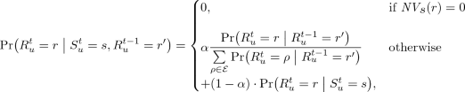(6)

where $\mathcal {E}= \{\rho \in \mathcal {R}: NV _{s}(\rho ) > 0\}$ and $\alpha$ is a real-valued parameter that is used to set the weight of each term in the equation. The distributions $\Pr \bigl ( S_{u}^t\bigm \vert S_{u}^{t-1} \bigr )$ and $\Pr \bigl ( R_{u}^t\bigm \vert R_{u}^{t-1} \bigr )$ can be learned from the prior traces by applying maximum likelihood estimation (if the traces are complete) or by using algorithms such as Gibbs sampling (if the traces have missing locations or if they are noisy) [6, 20, 23]. The distribution $\Pr \bigl ( R_{u}^t\bigm \vert S_{u}^t\bigr )$ can also be learned from the prior traces. More precisely, $\Pr \bigl ( R_{u}^t=r\bigm \vert S_{u}^t=s\bigr )$ can be estimated by counting in the user’s prior traces, the number of visits to a region $r$ given the semantic tag $s$ [1]. Note that in the experimental evaluation in [1], Ağir et al. set $\alpha$ $=$ 0.5 to accord the same importance to both terms of the equation. In this paper, we also set $\alpha$ $=$ 0.5 for the experimental evaluation.

$\bullet$ :

The initial state distributions: $\varvec{\Pr \bigl ( R_{u}^1 \bigm \vert S_{u}^1 \bigr )}$ and $\varvec{\Pr \bigl ( S_{u}^1)}$. These are the distributions associated to the nodes of the first time slice of the model. For the estimation of $\Pr \bigl ( R_{u}^1 \bigm \vert S_{u}^1 \bigr )$, we refer the reader to the previous point, where we discuss the estimation of $\Pr \bigl ( R_{u}^t\bigm \vert S_{u}^t\bigr )$ from the prior traces (recall that the model is time-invariant). Moreover, we assume that $\Pr \bigl ( S_{u}^1)$ is equal to the stationary distribution of the Markov chain $S_{u}^{1:T}$. Accordingly, it can be found based on $\Pr \bigl ( S_{u}^t\bigm \vert S_{u}^{t-1} \bigr )$, which is the transition distribution of the chain. We refer the reader to the previous point where we discuss the estimation of $\Pr \bigl ( S_{u}^t\bigm \vert S_{u}^{t-1} \bigr )$ from the prior traces.

3.1.2 The DBNs for the Obfuscation Approaches

Figure 3.b depicts the DBN built for user $u$ in the case where the PPM uses the disjoint obfuscation approach. Also, Fig. 3.c depicts the DBN built for user $u$ in the case where the PPM uses the joint obfuscation approach. Each of these DBNs is made by adding the observed variables $\widetilde{R}_{u}^{1:T}$ and $\widetilde{S}_{u}^{1:T}$ to the basic DBN, where the observed variables correspond to the obfuscation approach used by the PPM. Note that in the DBN model built for the joint approach, to represent the fact that in the joint obfuscation, $\widetilde{R}_{u}^t$ depends also on $\widetilde{S}_{u}^t$, an edge connects the corresponding nodes in each time slice t of the model (See Fig. 3.c).

Parameters. Each of these models is fully specified by the parameters of the basic DBN plus the observation distributions. The observation distributions of a model are the CPDs that define the probabilistic dependencies between the hidden and the observed variables in any time slice t in that model. The observation distributions of a model are defined based on the obfuscation approach used by the PPM. So, we have:

$\bullet$ :

The observation distributions for the disjoint obfuscation case: $\varvec{\Pr \bigl ( \widetilde{S}_{u}^t\bigm \vert S_{u}^t\bigr )}$ and $\varvec{\Pr \bigl ( \widetilde{R}_{u}^t\bigm \vert R_{u}^t\bigr )}$. These are in fact the obfuscation functions of the PPM in the disjoint obfuscation approach (see Eqs. 1 and 2), and hence known by the adversary.

$\bullet$ :

The observation distributions for the joint obfuscation case: $\varvec{\Pr \bigl ( \widetilde{S}_{u}^t\bigm \vert S_{u}^t\bigr )}$ and $\varvec{\Pr \bigl ( \widetilde{R}_{u}^t\bigm \vert R_{u}^t, \widetilde{S}_{u}^t\bigr )}$. These are in fact the obfuscation functions of the PPM in the joint obfuscation approach (see Eqs. 3 and 4), and hence known by the adversary.

4 Location Privacy Metric

The location privacy of a user $u$ a time t is measured by the expected error of the adversary when performing the location-inference attack [23]. The expected error of the adversary is computed as:

$$\begin{aligned} \sum \limits _{r\in \mathcal {R}}\Pr \bigl ( R_{u}^t=r\bigm \vert \tilde{r}_{u}^{1:T}, \tilde{s}_{u}^{1:T}\bigr )\cdot d_{loc }(r,r_{u}^t) \end{aligned}$$

(7)

where $\Pr \bigl ( R_{u}^t=r\bigm \vert \tilde{r}_{u}^{1:T}, \tilde{s}_{u}^{1:T}\bigr )$ over set $\mathcal {R}$, is the output of the location-inference attack defined in Sect. 2 and $d_{loc }$($\cdot$,$\cdot$) denotes a distance function on the set $\mathcal {R}$ of regions. Here, we assume that $d_{loc }$($\cdot$,$\cdot$) is the Haversine distance between the centers of the two regions [14].

5 Experimental Evaluation

Using a dataset of real-world user mobility traces, we perform an experimental evaluation to compare the performance of the joint approach with the performance of the disjoint approach in terms of location privacy protection. We also study the impact of different obfuscation parameters on the performance of these approaches. More precisely, we first obfuscate the user traces under the disjoint and the joint approaches using different combinations of the obfuscation parameters. Then, we perform the location-inference attack on the obfuscated traces and measure the location privacy of users in both approaches based on the results of the attack.

5.1 Evaluation Setup

In this section, we describe the evaluation’s setup.

5.1.1 Dataset and Space Discretization

We use the dataset that is introduced and described in [1]. It comprises the semantically-annotated location traces of Foursquare check-ins of 1065 users distributed across six large cities in North America and Europe [1]. The location information in the traces is presented as GPS coordinates. The dataset also contains a snapshot of Foursquare category tree at the time of data collection [1].

Regarding the space discretization, we use the same space discretization described in [1]. More precisely, within each city in the dataset, a geographical area of size $\sim$2.4 km $\times$ 1.6 km that contains the largest number of check-ins is selected. Then, each selected area is partitioned into 96 locations (cells) by using a $12~\times ~8$ regular square grid. Each grid cell has a unique ID. Once the partitioning is done, the GPS coordinates in user traces are mapped to the location, that is, the grid cell, they fall into. Moreover, for each grid cell, the Foursquare semantic tags of the venues that are located in that cell are identified and stored in an associative array. Thus, the associative array contains the key-value pairs, where in each pair the key is a grid cell ID and the value is the set of the semantic tags of the venues located in that cell.

5.1.2 Obfuscation

In the following, we first introduce the obfuscation algorithms used in our evaluation. We then describe the process of building the obfuscated traces from the real traces using these algorithms. In practice, these algorithms are implemented in Python.

Semantic Tag Obfuscation Algorithm. The semantic tag obfuscation in both disjoint and joint obfuscation approaches is performed by the semantic tag obfuscation algorithm described as below. The algorithm gets as input a set $\mathcal {S}$ of semantic tags that form a semantic tag tree, a semantic tag $s$ in $\mathcal {S}$ and a semantic tag obfuscation level ${o }_{sem }$. It returns as output a pseudo-semantic tag $\tilde{s}$, where $\tilde{s}$ is the ancestor of $s$ that is ${o }_{sem }$ level(s) above $s$ in the semantic tag tree. In the case where the depth of semantic tag $s$ in the semantic tag tree is smaller than ${o }_{sem }$, the algorithm returns the root of the semantic tag tree as $\tilde{s}$.

Location Obfuscation Algorithm. The location obfuscation in both disjoint and joint obfuscation approaches is performed by the location obfuscation algorithm. The algorithm takes as input a grid that we call the main grid for the sake of precision, a cell $r$ of the main grid, a location obfuscation level ${o }_{loc }$ and an obfuscation approach. In the case of joint obfuscation, in addition to what has been described, the following inputs should also be provided: the semantic tag tree that is used as input by the semantic tag obfuscation algorithm, the pseudo-semantic tag $\tilde{s}$ that is output by the semantic tag obfuscation algorithm and an associative array that contains key-value pairs where in each pair the key is a main grid cell ID and the value is the set of the semantic tags of the venues located in that cell. The algorithm returns as output a cloaking area $\tilde{r}$ for $r$.

The main idea behind the algorithm is to first find a set of potential cloaking areas for $r$ and then based on the obfuscation approach, select an area among the potential cloaking areas and return it as $\tilde{r}$. The algorithm finds the potential cloaking areas by building a set of cloaking grids. A cloaking grid is an alternative tessellation for the same surface presented by the main grid. It has two properties: (1) each cell of a clocking grid is made of ${o }_{loc }$ distinct cells of the main grid; (2) the number of rows and the number of columns of a cloaking grid are factors of the number of rows and the number of columns of the main grid, respectively. Each cloaking grid can be used to find a potential cloaking area for $r$. More precisely, the cell of a cloaking grid that contains $r$, is a potential clocking area for $r$ and can be added to the set of potential cloaking areas.

Once the potential cloaking areas are found, an area among them is selected and returned as $\tilde{r}$. The selection is made based on the obfuscation approach. More precisely, in the case of the disjoint obfuscation, the algorithm selects an area uniformly at random among the potential cloaking areas and returns it as $\tilde{r}$. In the case of the joint obfuscation, the algorithm first looks for the areas with the maximum $NCR _{\tilde{s}}$ value among the potential cloaking areas. The results are then stored in the set $CAsWithMaxNCR$. If only one area with the maximum $NCR _{\tilde{s}}$ value is found (i.e., $|CAsWithMaxNCR | = 1$), the algorithm returns it as $\tilde{r}$. Otherwise, the algorithm looks for the areas with the maximum $SumNCV _{\tilde{s}}$ value among the elements of $CAsWithMaxNCR$. The results are then stored in the set $CAsWithMaxSumNCV$. Note that the $SumNCV _{\tilde{s}}$ of an area is in fact the sum of $NCV _{\tilde{s}}$ values over all the main grid cells in that area. If only one area with the maximum $SumNCV _{\tilde{s}}$ value is found (i.e., $|CAsWithMaxSumNCV | = 1$), the algorithm returns it as $\tilde{r}$. Otherwise, the algorithm selects an area uniformly at random among the elements of $CAsWithMaxSumNCV$ and returns it as $\tilde{r}$.

Note that, selecting the area with the maximum $SumNCV _{\tilde{s}}$ value among the areas with the maximum $NCR _{\tilde{s}}$ value is an additional mechanism that we use to enhance the resistance of the joint obfuscation against the privacy attacks. Intuitively, by selecting the clocking area with the maximum $NCR _{\tilde{s}}$ value (i.e., the area with the maximum number of semantically compatible locations), we decrease the number of locations that can be filtered out by the adversary from the cloaking area and by selecting the cloaking area with the maximum $SumNCV _{\tilde{s}}$ value (i.e., the area with the maximum number of semantically compatible venues), we increase the number of locations and semantic tags that can be guessed by the adversary as the actual location and semantic tag.

Building the Obfuscated Traces. For each city in the dataset, we choose the location traces and the semantic tag traces of 20 randomly chosen users. These traces are then obfuscated under the disjoint and the joint obfuscation approaches using the obfuscation algorithms. To better capture the fact that the users do not share their locations and their corresponding semantic tags all the time on LBSNs, we apply the obfuscation algorithms with an additional hiding process. Thus, we assume that at each time instant in the observation interval, both the user’s location and its semantic tag can be hidden from the LBSN with the hiding probability $\lambda$ or shared on the LBSN (and accordingly obfuscated by the algorithms under the disjoint and the joint approaches) with the probability $1- \lambda$. The hidden locations and the hidden semantic tags are appeared in the obfuscated traces as hidden, denoted by $r_{\perp }$ and $s_{\perp }$ symbols, respectively. To build the obfuscated traces for each approach, we use all combinations of the following parameters: the location obfuscation level (${o }_{loc }$), the semantic tag obfuscation level (${o }_{sem }$) and the hiding probability ($\lambda$), where ${o }_{loc }\in \{ 1, 2, 4, 8, 16 \}$ and ${o }_{sem }\in \{ 0, 1, 2 \}$ and $\lambda \in \{ 0, 0.2, 0.4, 0.6, 0.8 \}$. Note that, in what follows, we use the term the obfuscation parameters to refer to these parameters.

5.1.3 Attack and Privacy Evaluation

We implement the DBN models in Python by using the pomegranate package [19] and the Bayesian Belief Networks library [3]. For the attack, we apply the loopy belief propagation inference algorithm [17]. We perform the attack for the observation interval of length 3. We then use the metric defined in Sect. 4 to measure the location privacy of the users.

5.2 Experimental Results

In this section we present the results for different values of the obfuscation parameters. In this way, we can compare the performance of the two obfuscation approaches in terms of location privacy under different values of these parameters and also show how changing these parameters can affect the performance of the approaches. Note that in addition to the location privacy metric presented in Sect. 4, to discuss the results, we use the following additional metric:

$\bullet$ :

Ratio of the location privacy means (denoted by $loc-priv-ratio$). This is the ratio of the location privacy mean obtained for the joint approach to the location privacy mean obtained for the disjoint approach.

Fig. 4.

Location privacy results.

Fig. 5.

$loc-priv-ratio$ for different values of the obfuscation parameters.

The evaluation results are depicted by Fig. 4 and Fig. 5. More precisely, Fig. 4 represents the location privacy results in the form of boxplots (i.e., first quartile, median, third quartile and outliers). Note that the location privacy in Fig. 4 is expressed in kilometres. Also, Fig. 5 represents the ratios of the location privacy means in the form of scatterplots. Each figure has three subfigures (a), (b) and (c). Each subfigure represents the aggregated results for different values of a given obfuscation parameter, where the aggregation is performed over the results obtained for all users, all values of the obfuscation parameters and all cities. We have three main observations regarding these results. Thus, in the following we first describe the observations. Then, we describe the reason behind the observations.

• 1. As the values of ${o }_{loc }$, ${o }_{sem }$ and $\lambda$ increase, the median location privacy for the both obfuscation approaches increases (see subfigures (a),(b),(c) of Fig. 4).

• 2. Under all values of ${o }_{loc }$, ${o }_{sem }$ and $\lambda$, the median location privacy obtained for the joint approach is higher than the median location privacy obtained for the disjoint approach (see subfigures (a),(b),(c) of Fig. 4). The only exception to this observation is the case where ${o }_{loc }= 1$ (See Fig. 4.a). In this case, no location obfuscation is performed and hence, the median location privacy is the same for the both obfuscation approaches.

• 3. As the values of ${o }_{loc }$ and ${o }_{sem }$ increase, the value of $loc-priv-ratio$ also increases (see Fig. 5.a and Fig. 5.b). However, as the value of $\lambda$ increases, the value of $loc-priv-ratio$ decreases (see Fig. 5.c).

To explain these observations, we apply the following reasoning. As the value of ${o }_{loc }$ increases, the number of regions (locations) in the cloaking area increases. Thus, by increasing ${o }_{loc }$, the median location privacy for the both approaches increases. Also, as the value of ${o }_{sem }$ increases, the number of semantic tags that can be semantically compatible with the obfuscated semantic tag increases. This, in turn, increases the chance of having more semantically compatible regions with the obfuscated semantic tag in every potential cloaking area. Thus, by increasing ${o }_{sem }$ the median location privacy for the both approaches increases. Moreover, we observe that by increasing ${o }_{loc }$ and ${o }_{sem }$, the value of $loc-priv-ratio$ also increases. Roughly speaking, this means that the joint approach shows a much better performance in terms of location privacy protection compared to the disjoint approach under higher values of ${o }_{loc }$ and ${o }_{sem }$. In fact, as the value of ${o }_{loc }$ increases, the number of candidate regions for being in the clocking area also increases. This, in turn, increases the chance that a greater number of the candidate regions are semantically compatible with the obfuscated semantic tag. Similarly, as the value of ${o }_{sem }$ increases, the chance that a greater number of candidate regions are semantically compatible with the obfuscated semantic tag increases. The joint approach takes advantage of this increase, i.e., as the number of semantically compatible candidate regions increases, the joint approach selects a cloaking area with a greater number of semantically compatible regions and semantically compatible venues, whereas the disjoint approach is oblivious to the concept of semantic compatibility. Accordingly, the performance of the disjoint approach does not improve as much as the performance of the joint approach by increasing the values of ${o }_{loc }$ and ${o }_{sem }$. We also observe that as the value of $\lambda$ increases, the median location privacy for the both approaches increases. However, by increasing $\lambda$, the value of $loc-priv-ratio$ decreases. Roughly speaking, this means that by increasing $\lambda$, the difference between the performance of the both approaches becomes less significant. Intuitively, this is because by increasing $\lambda$, we increase the number of hidden locations and hidden semantic tags compared to the number of the obfuscated locations and the obfuscated semantic tags in the obfuscated traces. This, in turn, increases the location privacies resulting for the both approaches but it also decreases the importance of the obfuscation approach in defining the amount of the resulting location privacies.

6 Related Work

The problem of protecting location privacy of users in LBSNs (and in LBSs, in general) has been extensively studied in the literature and various protection mechanisms are proposed. Many of the location privacy protection mechanisms apply location obfuscation. The popularity of the location obfuscation lies in the fact that it does not require changing the infrastructure, as it can be performed entirely on the user’s side [25]. There exist different methods to obfuscate a location, for instance, by hiding the location from the LBS [4, 8], by perturbing the location (e.g., by adding noise to the location coordinates) [2], by generalizing the location (e.g., by merging the location with nearby locations using a cloaking algorithm) [9, 10, 15, 26] and by adding fake (dummy) locations to the actual location [6, 7, 12, 27] (See [13, 21, 22] for detailed surveys on location obfuscation methods). Our work differs from these works by the fact that it considers not only the obfuscation of location but also the obfuscation of the semantic information to protect the location privacy. In addition, the location obfuscation in our work is performed with respect to the obfuscated semantic information, whereas the location obfuscation in these works is semantic-oblivious.

The disjoint obfuscation approach discussed in this paper, was originally introduced in [1]. Our work is close to the work presented in [1], in the sense that it assumes a similar system model and adversary model. In fact, our work and the work in [1] are both built upon the Shokri’s framework for quantifying location privacy [20, 23, 24]) and they both rely on bayesian network models for implementing the inference attacks. However, as already discussed, in this paper we try to improve the work in [1], by proposing a joint obfuscation approach. Another difference between this paper and the work presented in [1] is the fact that, in [1], the authors study the impact of the location obfuscation and the semantic tag obfuscation on both location privacy and the semantic location privacy of users, whereas in this paper we only discuss the impact of the location obfuscation and the semantic tag obfuscation on location privacy. We intend to discuss the impact on semantic location privacy in a future work.

7 Conclusion

In this paper, we have introduced a joint semantic tag-location obfuscation approach for privacy protection in LBSNs. This approach aims to overcome the drawbacks of the existing disjoint approach, by performing the location obfuscation based on the result of the semantic tag obfuscation. We provided a formal framework for evaluation and comparison of the joint approach with the disjoint approach. Then, using a dataset of real-world user mobility traces, we performed an experimental evaluation. The evaluation results show that in almost all cases (i.e., for different values of the obfuscation parameters), the joint approach outperforms the disjoint approach in terms of location privacy protection. We also studied the impact of changing different obfuscation parameters on the obfuscation approaches. In particular, we showed that compared to the disjoint approach, the joint approach can take better advantage of higher values of location obfuscation level and semantic tag obfuscation level and exhibits even more satisfactory performance under higher values of these parameters.

References

Ağir B., Huguenin, K., Hengartner, U., Hubaux, J.-P.: On the privacy implications of location semantics. In: PoPETs Journal (2016)
Andrés, M.E., Bordenabe, N.E., Chatzikokolakis, K., Palamidessi, C.: Geo-indistinguishability: differential privacy for location-based systems. In: ACM SIGSAC 2013 (2013)
eBay/BBN library.https://github.com/eBay/bayesian-belief-networks
Beresford, A., Stajano, F.: Location privacy in pervasive computing. In: IEEE Pervasive Computing (2003)
Bilogrevic, I., Huguenin, K., Mihaila, S., Shokri, R., Hubaux, J.-P.: Predicting users motivations behind location check-ins and utility implications of privacy protection mechanisms. In: NDSS 2015 (2015)
Bindschaedler, V., Shokri, R.: Synthesizing plausible privacy-preserving location traces. In: S & P 2016 (2016)
Chow, R., Golle, P.: Faking contextual data for fun, profit, and privacy. In: ACM WPES 2009 (2009)
Freudiger, J., Shokri, R., Hubaux, J.-P.: On the optimal placement of mix zones. In: PETS 2009 (2009)
Gedik, B.: Location privacy in mobile systems: a personalized anonymization model. In: ICDCS 2005 (2005)
Kalnis, P., Ghinita, G., Mouratidis, K., Papadias, D.: Preventing location-based identity inference in anonymous spatial queries. In: IEEE TKDE (2007)
Koller, D., Friedman, N.: Probabilistic Graphical Models: Principles and Techniques. The MIT Press, Cambridge (2009)
Krumm, J.: Realistic driving trips for location privacy. In: IEEE PerCom 2009 (2009)
Krumm, J.: A survey of computational location privacy. In: Personal Ubiquitous Computer (2009)
Olteanu, A.-M., Huguenin, K., Shokri, R., Humbert, M., Hubaux, J.-P.: Quantifying interdependent privacy risks with location data. IEEE Trans. Mob, Comput (2017)
Mokbel, M., Chow, C., Aref, W.: The new casper: query processing for location services without compromising privacy. In: VLDB 2006 (2006)
Murphy, K.P.: Dynamic Bayesian Networks: Representation, Inference and Learning. Ph.D. Thesis, UC Berkeley (2002)
Murphy, K.P., Weiss. Y., Jordan, M.: Loopy belief propagation for approximate inference: an empirical study. In: UAI (1999)
Pearl, J.: Probabilistic Reasoning in Intelligent Systems: Networks of Plausible Inference. M. Kaufmann (1988)
Pomegranate. https://pomegranate.readthedocs.io/en/latest/
Shokri, R.: Quantifying and Protecting Location Privacy. PhD. Thesis, EPFL (2012)
Shokri, R., Freudiger, J., Jadliwala, M., Hubaux, J.-P.: A distortion-based metric for location privacy. In: ACM WPES 2009 (2009)
Shokri, R., Freudiger, J., Hubaux, J.-P.: A unified framework for location privacy. In: HotPETs 2010 (2010)
Shokri, R., Theodorakopoulos, G., Le Boudec, J.-Y., Hubaux, J.-P.: Quantifying location privacy. In: IEEE S & P 2011 (2011)
Shokri, R., Theodorakopoulos, G., Danezis, G., Le Boudec, J.-Y., Hubaux, J.-P.: Quantifying location privacy: the case of sporadic location exposure. In: PETS 2011 (2011)
Shokri, R., Theodorakopoulos, G., Troncoso, C.: Privacy Games Along Location Traces: A Game-Theoretic Framework for Optimizing Location Privacy. In: ACM Trans. Priv, Secur (2016)
Xu, T., Cai, Y.: Feeling-based location privacy protection for location-based services. In: CCS 2009 (2009)
You, T., Peng, W., Lee, W.: Protecting moving trajectories with dummies. In: IEEE MDM 2007 (2007)
Acknowledgements
This research is partially funded by a UNIL/CHUV postdoc mobility grant disbursed by University of Lausanne and Lausanne University Hospital. We also thank Berker Ağir for his comments and help regarding the disjoint obfuscation approach.
Author information
Authors and Affiliations
Corresponding author
Editor information
Editors and Affiliations
Rights and permissions
Copyright information
© 2020 Springer Nature Switzerland AG
About this paper
Cite this paper
Bostanipour, B., Theodorakopoulos, G. (2020). Joint Obfuscation for Privacy Protection in Location-Based Social Networks. In: Garcia-Alfaro, J., Navarro-Arribas, G., Herrera-Joancomarti, J. (eds) Data Privacy Management, Cryptocurrencies and Blockchain Technology. DPM CBT 2020 2020. Lecture Notes in Computer Science(), vol 12484. Springer, Cham. https://doi.org/10.1007/978-3-030-66172-4_7
Download citation
DOI: https://doi.org/10.1007/978-3-030-66172-4_7
Published:
Publisher Name: Springer, Cham
Print ISBN: 978-3-030-66171-7
Online ISBN: 978-3-030-66172-4
eBook Packages: Computer ScienceComputer Science (R0)