Laminar Convection In Internal Flow

Abstract

In Chap. 1, we have introduced the concept of convection through a phenomenological description by introducing h, the convection heat transfer coefficient. The heat transfer coefficient was introduced through the so-called “Newton’s law of cooling”. In many problems encountered in conduction heat transfer, we have made use of a suitable “h” value to describe what happens at a boundary between a solid and the ambient fluid. However, no effort was made to describe the basis for choosing a particular value of h. In what follows we would like to calculate h by using fundamental heat transfer principles that are involved in the case of a flowing fluid.

We commence the study of convection heat transfer in this chapter. After looking at fluid properties of interest in convection heat transfer, we present notion of similarity to understand scaling principles that play a crucial role in convection heat transfer. Laminar fully developed flow and heat transfer in internal flows are covered in great detail. Useful relations are presented for heat transfer in the developing region.

12.1 Introduction

In Chap. 1, we have introduced the concept of convection through a phenomenological description by introducing h, the convection heat transfer coefficient. The heat transfer coefficient was introduced through the so-called “Newton’s law of cooling”. In many problems encountered in conduction heat transfer, we have made use of a suitable “h” value to describe what happens at a boundary between a solid and the ambient fluid. However, no effort was made to describe the basis for choosing a particular value of h. In what follows we would like to calculate h by using fundamental heat transfer principles that are involved in the case of a flowing fluid.

12.1.1 Classification of Flows

The main goal of the study of convection heat transfer is to understand the dependence of the convection heat transfer coefficient on (1) The nature of the fluid, (2) The nature of flow, and (3) The type of flow.

(1) The nature of fluid

Basically, the nature of the fluid is mirrored by its physical and transport properties. Also, the variation of these properties within the flow domain decides the method of analysis. The fluid may be described by any of the following models, depending on the circumstance.

 

Incompressible fluid::

Fluid density remains fixed irrespective of variations in pressure and temperature.

Compressible fluid::

Fluid density varies with position and time due to changes in pressure or temperature. In high speed flows (flow speed comparable to the speed of sound in the fluid), the compressibility effects may become significant. However, the same fluid may be treated as incompressible if the fluid speed is small compared to the speed of sound in the medium.

Inviscid or non-viscous and non-heat conducting fluid::

This is also referred to as an ideal fluid. A flow, far away from boundaries, even when the fluid has a non-zero viscosity, may sometimes be treated this way.

Viscous and heat conducting fluid::

The fluid is referred to as a real fluid. As a subset of this, the fluid may be Newtonian or non-Newtonian. Newtonian fluid has a linear relationship between shear stress and velocity gradient while the non-Newtonian fluid has a more complex relationship. We consider only a Newtonian fluid in this text.

Fluid with constant thermo-physical properties::

For such a fluid the properties like viscosity and thermal conductivity have very insignificant variation with temperature and pressure. In flows with small variation of temperature constant, property assumption may be justified.

Fluid with variable thermo-physical properties::

The fluid properties such as viscosity and thermal conductivity vary significantly in the flow domain. Most important variation that needs to be considered is with respect to fluid temperature. Variation with pressure is seldom significant. Constant property assumption is not necessarily connected with the variation or otherwise of the fluid density.

 

(2) Nature of flow and attendant heat transfer

The nature of the flow is important since it affects heat transfer to a great extent. In practical applications, it is usual to look for flow conditions that enhance heat transfer significantly in comparison with conduction heat transfer that will take place in a stationary fluid.

 

Compressible high-speed flow::

High speed means M, the Mach number (the ratio of fluid velocity to the speed of sound in the fluid) is large. Incompressible, low speed flow approximation is valid, in gases, for $M\le 0.3$.

Laminar flow::

Laminar flow is orderly or “streamline” flow. Laminar flow is also characterized by weak mixing except in regions of flow close to boundaries.

Turbulent flow::

Turbulent flow exhibits temporal variations in velocity and temperature fields even when the flow is steady. Rapid mixing normal to the flow direction is a characteristic of turbulent flow.

Forced Convection::

Flow is created or forced to take place by an external agency like a pump. The pump creates a pressure gradient that promotes and maintains the flow.

Free or natural convection::

Flow is generated by temperature differences and the consequent density differences within the flowing medium. The flow may be assumed to be incompressible except for the buoyancy effect.

Mixed convection::

Forced and free convection occur simultaneously and are of comparable importance. The buoyancy effects may either aid or oppose the forced flow.

 

(3) Type of Flow

The flow may also be classified according to the following types.

 

Internal Flow::

Flow inside tubes and ducts. These occur in applications such as air handling systems, heat exchangers, energy conversion devices like turbines, engines, etc.

External Flow::

Flow over extended surfaces, flow past a tube bundle in a heat exchanger, flow past vehicles, etc.

Steady flow::

Velocity and temperature fields do not change with time.

Unsteady flow::

Velocity and temperature fields change with time.

 

12.1.2 Fluid Properties and Their Variation

Thermo-physical properties of the fluid influence flow and the consequent heat transfer. Details of flow and temperature fields are affected by the properties as well as their variations with temperature and pressure of the flowing fluid. Hence, we shall look at some of the important thermo-physical properties and their variations with temperature and pressure in this section.

(1) Fluid Viscosity

For a Newtonian fluid, the dynamic viscosity $\mu$ is defined through a linear relation between the shear stress and the velocity gradient.

$$\begin{aligned} \boxed {\tau =\mu \frac{dv}{dy}} \end{aligned}$$

(12.1)

Fig. 12.1

Viscosity of a Newtonian fluid

Here, $\tau =$ shear stress, $\mu =$ dynamic viscosity, $v=$ velocity, $y=$ coordinate normal to v. The velocity field varies with y as shown in Fig. 12.1 when a viscous fluid flows past a boundary. The fluid at lower velocity tends to decelerate the flow with a higher velocity. The unit of dynamic viscosity $\mu$ is given by

$$\begin{aligned} \boxed {[\mu ] = \frac{{[\tau ]}}{{\frac{{dv}}{{dy}}}} = \frac{{\frac{{\mathrm {N}}}{{{\mathrm {m}}^{{\mathrm {2}}} }}}}{{\frac{{{\mathrm {m}}/{\mathrm {s}}}}{{\mathrm {m}}}}} = \frac{{{\mathrm {kg}}}}{{{\mathrm {m}}\;{\mathrm {s}}}} = \left[ {\frac{M}{{LT}}} \right] } \end{aligned}$$

(12.2)

In Eq. 12.2, the brackets indicate that the unit of the quantity within the brackets is being considered and not the magnitude. The last entry indicates the dimensions as will be explained later on.

Newton’s law of viscosity resembles Hooke’s law in solid mechanics and Fourier law of thermal conduction. For gases, $\mu$ increases with temperature. At 300 K, air has a dynamic viscosity of $18.46\times 10^{-6}$ kg/m s which increases to $42.4\times 10^{-5}$ kg/m s when the temperature changes to 1000 K. Dynamic viscosity of liquids decrease with temperature. For saturated liquid water, the dynamic viscosity decreases from $8.67\times 10^{-4}$ kg/m s at 300 K to $9.01\times 10^{-5}$ kg/m s at 573 K.

(2) Kinematic Viscosity

This is defined as the ratio of dynamic viscosity of the fluid and its density $\rho$.

$$\begin{aligned} \boxed {\nu =\frac{\mu }{\rho }} \end{aligned}$$

(12.3)

It may be verified that the unit of kinematic viscosity is m$^2$/s. The reader may note that the same unit also characterizes the thermal diffusivity encountered in conduction heat transfer. Generally, the kinematic viscosity of gases increases with temperature. However, for liquids, the kinematic viscosity decreases with temperature. For example, the kinematic viscosity of air increases from $15.89\times 10^{-6}$ m$^2$/s at 300 K to $12.9\times 10^{-5}$ m$^2$/s at 1000 K. The kinematic viscosity of saturated water decreases from $8.004\times 10^{-7}$ m$^2$/s at 303 K to $1.265\times 10^{-7}$ m$^2$/s at 573 K.

(3) Fluid Thermal Conductivity

Fourier law (already familiar to us from conduction heat transfer study) introduces the conductivity of the fluid. The unit of thermal conductivity is either W/m $^\circ \mathrm{C}$ or W/m K. Thermal conductivity of gases increases with temperature while it may show increasing as well as decreasing trends in the case of liquids. Examples are given in Table 12.1.

Table 12.1 Variation of thermal conductivity with temperature

(4) Thermal Diffusivity of a Fluid

This is defined in the usual way as $\alpha =\frac{k}{\rho c}$ where c is the specific heat capacity of the fluid in J/kg $^\circ \mathrm{C}$ or J/kg K. Thermal diffusivity has the units of $m^2/s$.

(5) Prandtl Number

The ratio of kinematic viscosity to thermal diffusivity occurs very often in heat and fluid flow problems and hence is given a specific name, the Prandtl number, Pr. ¹ Thus,

$$\begin{aligned} \boxed {Pr=\frac{\nu }{\alpha }=\frac{\mu /\rho }{k/\rho c} =\frac{\mu c}{k}} \end{aligned}$$

(12.4)

It has no dimensions. The ranges of Pr values are given in Table 12.2.

Table 12.2 Ranges of Prandtl number of various fluids

Table 12.3 shows Prandtl number variation for two common liquids.

Table 12.3 Prandtl number of two common liquids

Fig. 12.2

a Variation of properties of air with temperature b Variation of properties of saturated liquid water with temperature

Since air and water are commonly used in heat transfer applications, their property variations with temperature are shown in Fig. 12.2a, b on p. xx. While the properties are for air at 1 atm, the properties of water are for saturated water at the indicated temperatures. Prandtl number of air varies very little with temperature and hence is not included in Fig. 12.2a. However, Prandtl number of water varies significantly with temperature and hence has been included in Fig. 12.2b.

12.2 Dimensional Analysis and Similarity

Non-dimensional parameters are useful in discussing the behavior of thermal systems. They naturally evolve while solving the governing differential equations, as we have already seen in the case of conduction problems. We have already seen how parameters such as the Biot and Fourier numbers evolve while solving conduction problems in one and two dimensions. We have introduced a non-dimensional parameter, the Prandtl number in Sect. 12.1. Many more non-dimensional parameters become appropriate in fluid flow and heat transfer problems. These are discussed with the concept of similarity in mind. Similarity may be of two types:

• 1. Geometric similarity

• 2. Dynamic similarity

  • involves motion, forces, temperatures, heat fluxes, etc.

These two concepts are elucidated below using examples from fluid flow and heat transfer.

12.2.1 Dimensional Analysis of a Flow Problem

The first example we consider is a flow problem in which a viscous fluid flows steadily through a straight tube of circular cross section. Two fluid flow situations are shown in Fig. 12.3. At the left is a circular tube of diameter $D_1$ carrying a fluid 1. At the right is a circular tube of diameter $D_2$ carrying a fluid 2. Geometric similarity would require that both be circular tubes. If one tube is straight, the other also should be straight. However, dynamic similarity requires that suitable non-dimensional parameters remain the same for the two cases.

Fig. 12.3

Pressure drop in a fluid flowing in a straight tube

Table 12.4 Physical quantities and their dimensions

The quantity of interest to us is the pressure drop between stations 1 and 2 or stations $1'$ and $2'$ . We first identify all the variables that enter the problem and also write out the units of these variables, using the SI system of units and also the length, mass, time system (refer to Table 12.4). In this last method, [M] will represent mass dimension, [L] will represent length dimension, and [T] will represent time dimension. Buckingham $\pi$ theorem ($\pi$ theorem because each non-dimensional parameter was represented by the symbol $\pi$) states that the number of non-dimensional parameters that characterize the problem are $(n-r)$ where “n” is the number of variables (= 6 in the present case) and “r” is the number of primary dimensions involved (= 3; Mass, Length, Time or [M], [L] and [T]).² Thus, we expect three non-dimensional parameters to characterize the problem. In order to obtain these parameters, we represent $\Delta p$ as a function of all the other variables that occur in the problem. Thus,

$$\begin{aligned} \Delta p=f(\rho ,\mu ,V,L,D) \end{aligned}$$

(12.5)

It is possible as it happen many times that the functional relation is of the type

$$\begin{aligned} f(\rho ,\mu ,V,L,D)=K\left\{ \rho ^a\mu ^bv^cL^dD^e\right\} \end{aligned}$$

(12.6)

where K is a numerical constant and a, b, c, d, e are numerical exponents. If indeed this is valid, then the unit of $\Delta p$ must be the same as the unit of the quantity inside the flower brackets in Eq. 12.6. This may be written using units of various quantities as

$$\begin{aligned} {\begin{matrix} {\mathrm {Units}}:\left( {\frac{{{\mathrm {kg}}}}{{{\mathrm {m}}\;{\mathrm {s}}^{2} }}} \right) = \left( {\frac{{{\mathrm {kg}}}}{{{\mathrm {m}}^{3} }}} \right) ^{a} \left( {\frac{{{\mathrm {kg}}}}{{{\mathrm {m}}\;{\mathrm {s}} }}} \right) ^{b} \left( {\frac{{\mathrm {m}}}{{\mathrm {s}}}} \right) ^{c} ({\mathrm {m}})^{d} ({\mathrm {m}})^{e}\\ \text {Dimensions:}\;\left[ \frac{M}{LT^2}\right] ^1=\left[ \frac{M}{L^3}\right] ^a \left[ \frac{M}{LT}\right] ^b\left[ \frac{L}{T}\right] ^c[L]^d[L]^e&{}\end{matrix}} \end{aligned}$$

(12.7)

Dimensional homogeneity requires that the left-hand side and right-hand side of Expression 12.7 have identical dimensional units. This will require the right choice of all the exponents $a-e$. This may be done by equating the exponent of each primary dimension mass, length, and time on the two sides. These lead to the following three equations:

$$\begin{aligned} \boxed {\text {(a)}\mathrm{[M]:} 1=a+b}\boxed {\text {(b)}\mathrm{[L]}:\; -1=-3a-b+c+d+e}\boxed {\text {(c)}\mathrm{[T]}:\; -2=-b-c} \end{aligned}$$

(12.8)

There are only 3 equations (number of equations is equal to the number of primary dimensions) but 5 unknowns. Hence, we solve for any 3 of them in terms of the other two. In this case, exponents $b,\;d$ are chosen as the two that may be assigned arbitrary/suitable numerical values and exponents $a,\; c,\; e$ are solved in terms of them. From Eq. 12.8(a) we have $a = 1 - b$. From Eq. 12.8(c), we have $c = 2 - b$. Substitute these in Eq. 12.8(b) to get

$$\begin{aligned} e=3a + b - c - d - 1 =3(1 - b) + b - (2 - b) -d -1=-b-d \end{aligned}$$

With these Eq. 12.5 may be rewritten, using Eq. 12.6 as

$$\begin{aligned} \Delta p=K\rho ^{1-b}\mu ^{b}V^{2-b}L^dD^{-b-d} =K\left( \frac{\mu }{\rho vD}\right) ^b\left( \frac{L}{D}\right) ^d\rho V^2 \end{aligned}$$

(12.9)

or, on rearrangement,

$$\begin{aligned} \boxed {\frac{\Delta p}{\rho V^2}=K\left( \frac{\mu }{\rho vD}\right) ^b \left( \frac{L}{D}\right) ^d \text {or} Eu=KRe_D^{-b}\left( \frac{L}{D}\right) ^d} \end{aligned}$$

(12.10)

Dimensional analysis cannot give the values of K, b, and d. They have to be determined from solution of appropriate equations that govern the fluid flow problem or from experiments. Both these alternates are used in practice. These will be presented later on.

We notice that Eq. 12.10 contains three non-dimensional parameters. They are

• Euler number Eu:

  $$\begin{aligned} Eu=\frac{\Delta p}{\rho V^2} \end{aligned}$$

  (12.11)

  Euler number is nothing but a non-dimensional pressure drop that uses the “dynamic head” $\frac{\rho V^2}{2}$ as the reference pressure drop. The factor $\frac{1}{2}$ may appropriately be absorbed in the coefficient K.

• Reynolds number $Re_D$:

  $$\begin{aligned} Re_D=\frac{\rho VD}{\mu } \end{aligned}$$

  (12.12)

  The subscript D is used to indicate that the Reynolds number is based on diameter of tube as the characteristic “length scale” in the problem.

• Length to diameter ratio or the non-dimensional length $L'$:

  $$\begin{aligned} L'=\frac{L}{D} \end{aligned}$$

  (12.13)

12.2.2 Notion of “Similarity”

Equation 12.9 may be interpreted as follows using the concept of similarity. Apart from the geometric similarity that was alluded to earlier, dynamic similarity requires additional conditions to be satisfied. For example, if we compare the two cases shown in Fig. 12.3 with $L_1,D_1$ fluid 1 and $L_2,D_2$ fluid 2, the non-dimensional pressure drop

$$\begin{aligned} \frac{\Delta p_1}{\rho _1 V_1^2}=\frac{\Delta p_2}{\rho _2 V_2^2}\;\text {or}\;Eu_1=Eu_2 \end{aligned}$$

(12.14)

if and only if

$$\begin{aligned} \text {(a)}\;\frac{\rho _1 V_1D_1}{\mu _1}=\frac{\rho _2 V_2D_2}{\mu _2}\text {or}Re_{D_1} =Re_{D_2}; \text {(b)} \frac{L_1}{D_1}=\frac{L_2}{D_2} \end{aligned}$$

(12.15)

Alternately, we may state that dynamic similarity exists if and only if the Reynolds numbers and length to diameter ratios are the same in the two cases. A typical example shows the utility of this concept.

Example 12.1

Air at atmospheric pressure and at a temperature of 300 K flows in a 2 m long smooth circular tube of 25 mm inner diameter. The velocity is adjusted such that the Reynolds number is 15,000. What is the velocity? What is the mass flow rate? The pressure drop is measured to be 100 Pa. If the fluid flowing in the tube is replaced by water at 300 K what will be the mass flow rate and the corresponding pressure drop?

Solution:

Step 1:

Since the concept of similarity applies to the cases, the following parameters are common to both cases.

$\underline{\text {Case (a) Fluid is air}}$

Step 2:

The air properties are taken from table of properties at $T=300$ K. All quantities are shown with a subscript 1 to indicate that the fluid is air.

$$\begin{aligned} \rho _1=1.1614\;\mathrm{kg}/\mathrm{m}^3;\;\nu _1=15.89\times 10^{-6}\;\mathrm{m}^2/\mathrm{s} \end{aligned}$$

Step 3:

Using the given value of Reynolds number, air velocity in the tube is

$$\begin{aligned} V_1=\frac{Re_{D_1}\nu _1}{D_1} =\frac{15000\times 15.89\times 10^{-6}}{0.025} =9.534\;\mathrm{m}/\mathrm{s} \end{aligned}$$

Step 4:

The mass flow rate of air is then given by

$$\begin{aligned} \dot{m}=\rho _1\cdot \frac{\pi D_1^2}{4}\cdot V_1= 1.1614\times \frac{\pi \times 0.025^2}{4}\times 9.534 =0.00545\;\mathrm{kg}/\mathrm{s} \end{aligned}$$

Step 5:

It is given that the pressure drop has been measured with air as $\Delta p_1=100$ Pa. Hence, the Euler number (the non-dimensional pressure drop) may be calculated as

$$\begin{aligned} Eu_1=\frac{\Delta p_1}{\rho _1V_1^2} =\frac{100}{1.1614\times 9.534^2}=0.9473 \end{aligned}$$

$\underline{\text {Case (b) Fluid is water}}$

Step 6:

The properties of water are taken from tables of properties at 300 K. All quantities are shown with a subscript 2 to indicate that the fluid is water.

$$\begin{aligned} \rho _2=995.7\;\mathrm{kg}/\mathrm{m}^3;\;\nu _2=8.004\times 10^{-7}\;\mathrm{m}^2/\mathrm{s} \end{aligned}$$

Step 7:

Using the given value of Reynolds number, water velocity in the tube is

$$\begin{aligned} V_2=\frac{Re_{D_2}\nu _2}{D_2} =\frac{15000\times 8.004\times 10^{-7}}{0.025} =0.48\;\mathrm{m}/\mathrm{s} \end{aligned}$$

Step 8:

The mass flow rate of water is then given by

$$\begin{aligned} \dot{m}=\rho _2\cdot \frac{\pi D_2^2}{4}\cdot V_2= 995.7\times \frac{\pi \times 0.025^2}{4}\times 0.48 =0.235\;\mathrm{kg}/\mathrm{s} \end{aligned}$$

Step 9:

The two cases satisfy dynamic similarity since the length to diameter ratio and the Reynolds number are unchanged. Hence, the Euler number is the same for the two cases. With this, we can calculate the pressure drop with water as

$$\begin{aligned} \Delta p_2=\rho _2V_2^2Eu_2= \rho _2V_2^2Eu_1=995.7\times 0.48^2\times 0.9473=217.3\;\mathrm{Pa} \end{aligned}$$

12.2.3 Dimensional Analysis of Heat Transfer Problem

Consider fluid flow in a tube with heat addition to the fluid as shown in Fig. 12.4.

Fig. 12.4

Tube flow with heat addition

We shall think of some average temperature difference $\Delta T_\mathrm{ref}$ as a representative temperature difference applicable to this problem. Then, we can define a suitable mean heat transfer coefficient h based on a representative area $S_\mathrm{ref}$ as $h=\frac{Q}{S_\mathrm{ref}\Delta T_\mathrm{ref}}$. Variables entering the problem along with their dimensions are given in Table 12.5.

Table 12.5 Physical quantities and dimensions

The tube length drops out of consideration since our interest is on the mean heat transfer coefficient defined for the entire length of the tube. There are thus $r=7$ parameters that govern the problem. We use $n= 4$ in the $M, L, T,\theta$—mass, length, time, temperature—system. By Buckingham $\pi$ theorem, there are $n-r=7 - 4 = 3$ non-dimensional parameters that describe the problem. Let us assume that the functional relation we seek is of form

$$\begin{aligned} h=K\rho ^a\mu ^bV^cc^dk^eD^f \end{aligned}$$

(12.16)

Hence, the dimensional equation may be written in the form

$$\begin{aligned} \left[ \frac{M}{T^3\theta }\right] ^1=\left[ \frac{M}{L^3}\right] ^a \left[ \frac{M}{LT}\right] ^b\left[ \frac{L}{T}\right] ^c\left[ \frac{L^2}{T^2\theta }\right] ^d\left[ \frac{ML}{T^3\theta }\right] ^e[L]^f \end{aligned}$$

(12.17)

Dimensional homogeneity requires the following balances.

$$\begin{aligned}{}[M]\; \text {balance:}1 = a + b + e\; \text {or}\; b = (1 - a - e) \end{aligned}$$

(12.18)

$$\begin{aligned}{}[L]\; \text {balance:} 0 = -3a - b + c + 2d + e + f\; \text {or}\;f = +3a + b - c - 2d - e \end{aligned}$$

(12.19)

$$\begin{aligned}{}[T]\; \text {balance:} -3 = -b - c - 2d - 3e \end{aligned}$$

(12.20)

$$\begin{aligned}{}[\theta ]\; \text {balance:} -1 = -d -e \; \text {or}\; d = 1 - e \end{aligned}$$

(12.21)

There are 6 unknowns and 4 equations (equal to the number of fundamental units). We solve for four of the unknowns, b, c, d, f in terms of a and e. Using Eqs. 12.18 and 12.21 in Eq. 12.19 gives

$$\begin{aligned} f=3a+(1-a-e)-c-2(1-e)-e=2a-c-1 \end{aligned}$$

(12.22)

From Eq. 12.20, using Eq. 12.21, we have

$$\begin{aligned} b =3 - c - 2 (1 - e) - 3e=1-c-e \end{aligned}$$

Comparing this with Eq. 12.18, we conclude that $a=c$. Using this in Eq. 12.22, we finally get

$$\begin{aligned} f = 3a + (1 - a - e)- a -2(1 - e) -e = a - 1 \end{aligned}$$

(12.23)

Substituting all these back in Eq. 12.16, we have

$$\begin{aligned} h=K\rho ^a\mu ^{1-a-e}V^ac^{1-e}k^eD^{a-1} \end{aligned}$$

(12.24)

Grouping terms with the same exponent, Eq. 12.24 takes the form

$$\begin{aligned} h=K\left( \frac{\rho VD}{\mu }\right) ^a\left( \frac{k}{\mu c}\right) ^{1-e}\left( \frac{k}{D}\right) \;\text {or}\; \left( \frac{h D}{k}\right) =K\left( \frac{\rho VD}{\mu }\right) ^a\left( \frac{k}{\mu c}\right) ^{1-e} \end{aligned}$$

This may be recast in terms of non-dimensional groups as

$$\begin{aligned} \boxed {Nu_D=KRe_D^aPr^{e-1}} \end{aligned}$$

(12.25)

The above relation links the three non-dimensional parameters that are important in the problem. Two of these, the Reynolds number $Re_D=\frac{VD}{\nu }$ and the Prandtl number given by $Pr=\frac{\mu c}{k}$ are already familiar to us. The third non-dimensional parameter that appears here is the Nusselt number given by $Nu_D=\frac{hD}{k}$ which is based again on the tube diameter as the characteristic length.³ Note that the Nusselt number is similar to the Biot number that was defined in problems involving conduction with convection at a boundary. However, the Biot number is based on the solid thermal conductivity while the Nusselt number is based on the fluid thermal conductivity. Similarity, in this case means that the Nusselt number is invariant if and only if $f(Re_{D_1},Pr_1)=f(Re_{D_2},Pr_2)$. Note that $K,\;a$, and e are not obtainable by dimensional analysis alone. Either experiments or analysis will have to give these.

The Nusselt number may be given a physical interpretation. It is the ratio of two heat fluxes, the convective heat flux in the moving medium to the conductive heat transfer in the stationary fluid. We may easily verify this by writing the Nusselt number as

$$\begin{aligned} \boxed {Nu_D=\frac{hD}{k}=\frac{\left( h\Delta T_\mathrm{ref}\right) }{\left( {\dfrac{k\Delta T_\mathrm{ref}}{D}}\right) } =\frac{q_c}{q_k}} \end{aligned}$$

(12.26)

The numerator $q_c$ is a representative convective heat flux, and the denominator $q_k$ is a representative conductive heat flux. Since $Nu_D$ is invariably greater than unity, convection enhances heat transfer to a value bigger than the representative conductive flux.

Example 12.2

Consider the situation described in Example 12.1. It is estimated that the heat transfer coefficient with air is 46 W/m$^2$ K. The Prandtl number of the fluid is expected to affect the Nusselt number by a factor proportional to $Pr^{0.36}$. What will be the heat transfer coefficient when the fluid flowing in the tube is changed to water?

Solution:

The data specified in Example 12.1 is reproduced below for ready reference. These are fluid independent.

$$\begin{aligned} Re_{D_1}=Re_{D_2}=15{,}000,\;D_1=D_2=0.025\;\mathrm{m},L_1=L_2=2\;\mathrm{m} \end{aligned}$$

$\underline{\mathrm{Nusselt~number~with~air~as~the~fluid:}}$

The heat transfer coefficient with air as the fluid is given as $h_1=46$ W/m$^2$ K.

From table of properties of air, we have, at 300 K,

$$\begin{aligned} k_1=0.0267\;\mathrm{W}/\mathrm{m}\;\mathrm{K},Pr_1=0.71 \end{aligned}$$

The Nusselt number with air as the flowing medium is then calculated as

$$\begin{aligned} Nu_1=\frac{h_1D_1}{k_1}=\frac{46\times 0.025}{0.0267} =43.07 \end{aligned}$$

$\underline{\mathrm{Nusselt~number~with~water~as~the~fluid:}}$

Since the Reynolds number and the length to diameter ratio are held fixed, the Nusselt number is affected only by the change in the Prandtl number when the fluid is changed from air to water. We have the following property values for water at 300 K.

$$\begin{aligned} k_2=0.611\;\mathrm{W}/\mathrm{m}\;\mathrm{K}, Pr_2=5.9 \end{aligned}$$

Using similarity law given by Eq. 12.25, we may identify the exponent $e-1$ as 0.36. Hence, the Nusselt number, $Nu_2$ with water as the fluid follows the relation

$$\begin{aligned} \frac{Nu_2}{Nu_1}=\left( \frac{Pr_2}{Pr_1}\right) ^{0.36} =\left( \frac{5.9}{0.71}\right) ^{0.36}=2.143 \end{aligned}$$

Hence, the Nusselt number with water is

$$\begin{aligned} Nu_2=43.07\times 2.143=92.31 \end{aligned}$$

Heat transfer coefficient with water as the fluid is then obtained as

$$\begin{aligned} h_2=\frac{Nu_2k_2}{D_2} =\frac{92.31\times 0.611}{0.025}=2256\;\mathrm{W}/\mathrm{m}^2\;\mathrm{K} \end{aligned}$$

There is thus a dramatic increase in the heat transfer coefficient when the fluid is changed from air to water keeping all other things the same!

12.3 Internal Flow Fundamentals

Convection heat transfer involves an interaction between flow (velocity) and temperature fields. Hence, it is not possible to discuss convection heat transfer without a clear understanding of fundamentals of fluid flow. As mentioned earlier in Sect. 12.1 there are several ways of classifying a flow. Here our interest will be the steady flow of a real (viscous and heat conducting) incompressible fluid. We attempt to understand laminar flow. Subsequently, in a later chapter, the attention will be directed toward internal as well as external turbulent flow. Special cases like compressible flows will also be taken up later on in Chap. 17.

12.3.1 Fundamentals of Steady Laminar Tube Flow

Consider steady laminar fluid flow in a straight tube of circular cross section. Experiments indicate that Laminar flow prevails in the tube for $Re_D<2300$ based on the mean velocity U and the tube diameter D. Assume that the fluid enters the tube at $z=0$ with a uniform velocity profile, i.e., the velocity is uniform across the tube cross section. Thus, the velocity $u_z$ in the axial direction is equal to a constant given $u_z(r,0)=U=\text {constant}$.

Figure 12.5 shows the details of how the velocity profile changes from entry down the length of the tube. Because of viscosity, the fluid velocity becomes zero at the tube wall and the flow field varies with r and z as indicated. Boundary layer—non-uniform velocity region near the boundary is referred to as boundary layer—develops from the periphery of the tube such that the velocity profile is non-uniform in the boundary layer and uniform in the core. Since the velocity is ${<}U$ near the tube wall, the velocity in the core region is ${>}U$, to guarantee that the volume flow rate (the flow is incompressible) across the tube cross section is the same for all z. The boundary layer occupies the entire tube cross section for $z\ge L_\mathrm{dev}$, where $L_\mathrm{dev}$ is referred to as the entry length. Beyond $z =L_\mathrm{dev}$, the velocity profile remains invariant with respect to z. Thus, the velocity profile is a function of “r” only for $z>L_\mathrm{dev}$. Experiments and analysis indicate that the entry length depends on $Re_D$ and is given by

$$\begin{aligned} \boxed {\frac{L_\mathrm{dev}}{D}=0.05\; Re_D} \end{aligned}$$

(12.27)

Fig. 12.5

Fluid flow in a straight tube

The flow beyond $z=L_\mathrm{dev}$ is referred to as fully developed flow. Analysis of the flow in this region is fairly simple and will be done below by two methods. First method derives the appropriate equation governing fully developed tube flow starting from the first principles. The second method starts with the Navier Stokes (NS) equations presented in Appendix H and obtains the governing equation by simplifying them.

12.3.2 Governing Equation Starting from First Principles

The fluid element in the form of a cylinder

Consider force balance on a cylindrical fluid element as shown in Fig. 12.6a. The fluid element is located in the fully developed region, is of radius r and is of length $\Delta z$ as shown in the figure. Under the fully developed condition, there is no change in the velocity $u_z$ with z. Hence, the rate at which momentum enters the cylinder through the left face of the cylindrical fluid element is the same as that leaving through the right face. Hence, there is no net momentum change for the fluid across the element length dz. Thus, the forces that are acting on the fluid element are as shown in Fig. 12.6a. The forces are the pressure forces at the two end faces and the shear stress on the curved cylindrical portion. All forces involved are along the z-direction. Force balance requires the following:

Fig. 12.6

Sketches to help in force balance from first principles a cylindrical fluid element b cylindrical annular fluid element

$$\begin{aligned} \pi r^2\;p(z)+2\pi r\Delta z\;\tau =\pi r^2\;p(z+\Delta z) \end{aligned}$$

(12.28)

Note that the shear stress is shown pointing toward $+z$. The convention is that the axial velocity $u_z$ is an increasing function with r. Using Taylor expansion, we have

$$\begin{aligned} p(z+\Delta z=p(z)+\left. \frac{dp}{dz}\right| _z\;\Delta z+O(\Delta z^2) \end{aligned}$$

Inserting these in Eq. 12.28, we get

$$\begin{aligned} \pi r^2\;p(z)+2\pi r\Delta z\tau =\pi r^2\;p(z)+\left. \frac{dp}{dz}\right| _z\;\Delta z \end{aligned}$$

Assuming the fluid to be a Newtonian fluid, the shear stress is related to the derivative of velocity with respect to r as $\tau =\mu \frac{du_z}{dr}$. On substituting this in the previous equation and on simplification, taking limit as $\Delta z\rightarrow 0$, we get

$$\begin{aligned} \boxed { \frac{du_z}{dr}=\frac{r}{2\mu }\frac{dp}{dz}} \end{aligned}$$

(12.29)

We note that the governing equation is a first-order differential equation. This equation is also obtained if we integrate Eq. 12.32, once with respect to r!

Fluid element in the form of a thin cylindrical shell

Consider force balance on a cylindrical shell element of length $\Delta z$ and thickness $\Delta r$. The comments made while describing the cylindrical fluid element also apply in the present case. Thus, the forces are the pressure forces at the two ends and the shear stresses on the cylindrical portions. All forces involved are along the z-direction. Force balance requires the following:

$$\begin{aligned} 2\pi r\Delta r\;p(z)+2\pi \Delta z\;\left. (r\tau )\right| _{r+\Delta r}=2\pi r\Delta r\;p(z+\Delta z)+2\pi \Delta r\Delta z\;(r\tau )|_r \end{aligned}$$

(12.30)

Using Taylor expansion, we have

$$\begin{aligned} p(z+\Delta z)= & {} p(z)+\left. \frac{dp}{dz}\right| _z\;\Delta z+O(\Delta z^2) \\ \left. (r\tau )\right| _{r+\Delta r}= & {} \left. (r\tau )\right| _r+\left. \frac{d(r\tau )}{dr}\right| _r\; \Delta r+O(\Delta r^2) \end{aligned}$$

Inserting these in Eq. 12.30, we get

$$\begin{aligned} \begin{aligned} 2\pi r\Delta r\; p(z)+2\pi \Delta z\;\left[ (r\tau )|_r+\left. \frac{d(r\tau )}{dr}\right| _r\; \Delta r+O(\Delta r^2)\right] =\\2\pi r\Delta r\; \left[ p(z)+\left. \frac{dp}{dz}\right| _z\; \Delta z+O(\Delta z^2)\right]&+2\pi \Delta z\;(r\tau )|_r \end{aligned} \end{aligned}$$

On canceling common terms and the common multiplier $\Delta r\Delta z$, taking limit as $\Delta r\rightarrow 0$ and $\Delta z\rightarrow 0$, we get

$$\begin{aligned} \frac{d(r\tau )}{dr}=r\frac{dp}{dz} \end{aligned}$$

(12.31)

With the Newtonian fluid assumption, the above equation becomes

$$\begin{aligned} \boxed {\frac{d}{dr}\left( r\frac{du_z}{dr}\right) =\frac{r}{\mu }\frac{dp}{dz}} \end{aligned}$$

(12.32)

We note that the governing equation is a second-order ordinary differential equation.

12.3.3 Governing Equation Starting with the NS Equations

Equations of motion of an incompressible fluid in steady $\left( \frac{\partial }{\partial t}\equiv 0\right)$ laminar flow are given by the Navier Stokes Equations. The present case involves axisymmetric flow for which the appropriate equations are given by Eqs. H.31 and H.32 since we are considering only the flow problem here. In the fully developed region the velocity component $u_r\equiv 0$, the velocity $u_z$ is a function of only r. With these, the equation of continuity is identically satisfied. The r momentum equation (Eq. H.31) reduces on taking $u_r\equiv 0$ and $\frac{\partial u_z}{\partial z}=0$ to

$$\begin{aligned} -\frac{\partial p}{\partial r}=0 \end{aligned}$$

(12.33)

thus showing that the pressure is a function of z alone. The z momentum equation (Eq. H.32) then simplifies to

$$\begin{aligned} 0=-\frac{1}{\rho }\frac{dp}{dz}+\nu \frac{1}{r}\frac{d}{dr} \left( r\frac{du_z}{dr}\right) \end{aligned}$$

or, on rearrangement to

$$\begin{aligned} \frac{d}{dr}\left( r\frac{du_z}{dr}\right) =\frac{r}{\mu }\frac{dp}{dz} \end{aligned}$$

(12.34)

Note that, for obvious reasons, all partial derivatives are now changed to total derivatives. Equation 12.34 is identical to Eq. 12.32 derived from first principles.

12.3.4 Solution

The governing equation for fully developed flow requires two boundary conditions or one boundary condition depending on whether we use the second-order equation or the first-order equation. In the first case, the two boundary conditions are specified as

$$\begin{aligned} \text {Tube wall:}\;u_z=0\;\text {at}\;r=R; \text {Tube axis:} \;u_z\;\text {is finite at}\;r=0 \end{aligned}$$

(12.35)

The first of these boundary condition corresponds to “no slip” at the tube wall. In the second case, only the tube wall boundary condition needs to be imposed. The other conditions are automatically satisfied.

We may integrate Eq. 12.29 with respect to r, noting that $\frac{dp}{dz}$ is independent of r, to get

$$\begin{aligned} u_z(r)=\frac{1}{2\mu }\frac{dp}{dz}\frac{r^2}{2}+A \end{aligned}$$

(12.36)

where A is a constant of integration. In general, A could have been a function of z. However, it as well as $\frac{dp}{dz}$ cannot be functions of z since the velocity profile is invariant with respect to z. We apply the boundary condition at the tube wall. We then have

$$\begin{aligned} 0=\frac{1}{2\mu }\frac{dp}{dz}\frac{R^2}{2}+A \end{aligned}$$

(12.37)

Subtracting Eq. 12.37 from 12.36 the constant of integration gets eliminated and hence

$$\begin{aligned} u_z(r)=\frac{r^2}{4\mu }\frac{dp}{dz}-\frac{R^2}{4\mu }\frac{dp}{dz} =-\frac{R^2}{4\mu }\frac{dp}{dz}\left[ 1-\left( \frac{r}{R}\right) ^2\right] \end{aligned}$$

(12.38)

We notice that at $r = 0$, i.e., at the axis of the tube, $u_z$ has the maximum value given by, say $u_z(r=0)=u_\mathrm{max}$. The maximum value is obtained by putting $r=0$ in Eq. 12.38 as

$$\begin{aligned} u_\mathrm{max}=-\frac{R^2}{4\mu }\frac{dp}{dz} \end{aligned}$$

(12.39)

This will be a positive quantity if the pressure decreases in the direction of flow! Equation 12.38 may be recast in the non-dimensional form

$$\begin{aligned} \boxed {\frac{u_z}{u_\mathrm{max}}=1-\left( \frac{r}{R}\right) ^2} \end{aligned}$$

(12.40)

The relationship between velocity and radius is a parabolic relation and is referred to as the Hagen–Poiseuille solution.⁴ The average velocity U is defined such that the volume flow rate through the tube is $\dot{V}=\pi R^2U$. Note that U is also the uniform velocity at entry to the tube. To conserve mass flow across the tube this must also be equal to the volume flow rate at any z. The volume flow rate in the fully developed region may be obtained the fully developed velocity profile given by Eq. 12.40.

(12.41)

Using the parabolic velocity profile, taking $\frac{r}{R}$ as $\zeta$, the above expression becomes

$$\begin{aligned} \dot{V}=2\pi R^2u_\mathrm{max}\int \limits _0^1\left( 1-\zeta ^2\right) \zeta d\zeta =2\pi R^2u_\mathrm{max}\left. \left[ \frac{\zeta ^2}{2}-\frac{\zeta ^4}{4}\right] \right| _0^1=\frac{\pi R^2 u_\mathrm{max}}{2} \end{aligned}$$

(12.42)

Equating the volume flow rate obtained above with $\dot{V}=\pi R^2U$, we see that the mean velocity is just half the maximum velocity, i.e.,

$$\begin{aligned} \boxed {U=\frac{u_\mathrm{max}}{2}} \end{aligned}$$

(12.43)

The pressure gradient may now be obtained in terms of the mean velocity, using Eq. 12.39.

$$\begin{aligned} \frac{dp}{dz}= -\frac{4\mu u_\mathrm{max}}{R^2} =-\frac{8\mu U}{R^2} \end{aligned}$$

(12.44)

The pressure gradient is a constant as already indicated. Hence, we may write it as the ratio of pressure drop $\Delta p$ over a length L in the fully developed region. Thus, we also have

$$\begin{aligned} \frac{dp}{dz}=\frac{\Delta p}{L}=-\frac{8\mu U}{R^2} \end{aligned}$$

(12.45)

It is customary to define a Darcy friction factor f such that the pressure drop is given by

(12.46)

We notice then that $-f\frac{L}{2D}$ is the Euler number that was obtained by the use of Buckingham $\pi$ theorem in Sect. 12.2. We also note that the present analysis provides the undetermined exponents in the expression obtained by dimensional arguments. The friction factor may be expressed as

$$\begin{aligned} f=-\frac{\dfrac{\Delta p}{\rho U^2}}{\dfrac{L}{2D}}= \frac{\dfrac{8\mu UL}{R^2\rho U^2}}{\dfrac{L}{2D}}=\frac{\dfrac{32\mu U}{D^2\rho U^2}}{\dfrac{1}{2D}}=\frac{64\mu }{\rho U D}=\frac{64}{Re_D}\text {or}\boxed {f\;Re_D=64} \end{aligned}$$

(12.47)

using Eq. 12.45 and by noting that $R=\frac{D}{2}$. With these, we may write for the Euler number the relation

$$\begin{aligned} \boxed { Eu=\frac{32}{Re_D}\frac{L}{D}} \end{aligned}$$

(12.48)

Comparing this with Eq. 12.10, we identify the constant K as 32, exponent b as 1, and exponent d as 1.

Example 13.3

Engine oil at $20\,^\circ \mathrm{C}$ is made to flow in a tube of 12 mm diameter. What is the maximum mass flow rate if the Reynolds number is not to exceed 10? What is the pressure drop in a length of 10 m under this flow condition?

Solution:

Step 1:

The density and kinematic viscosity of engine oil are taken from table of properties.

$$\begin{aligned} \rho =885.23\;\mathrm{kg}/\mathrm{m}^3,\;\nu =0.0009\;\mathrm{m}^2/\mathrm{s} \end{aligned}$$

The tube diameter and length are given as $L=10\;\mathrm{m},\;D=12\;\mathrm{mm}\,=0.012\;\mathrm{m}$.The Reynolds number based on the diameter is taken as the limiting value of $Re_D=10$ given in the problem.

Step 2:

Velocity calculation: The mean velocity corresponding to this Reynolds number is obtained as

$$\begin{aligned} U=\frac{Re_D\;\nu }{D} =\frac{10\times 0.0009}{0.012}=0.75\;\mathrm{m}/\mathrm{s} \end{aligned}$$

Step 3:

The mass flow corresponding to this flow velocity is obtained as

$$\begin{aligned} \dot{m}=\rho \frac{\pi D^2}{4}U =885.23\times \frac{\pi \times 0.012^2}{4}\times 0.75=0.075\;\mathrm{kg}/\mathrm{s} \end{aligned}$$

Step 4:

Pressure drop calculation: It is seen that the flow is laminar. The friction factor is calculated, using Eq. 12.47 as

$$\begin{aligned} f=\frac{64}{Re_D}=\frac{64}{10}=6.4 \end{aligned}$$

The flow development length is calculated based on Eq. 12.27 as

$$\begin{aligned} L_\mathrm{dev}=0.058Re_DD=0.058\times 10\times 0.012=0.00696\;\mathrm{m} \end{aligned}$$

The tube length of 10 m is much much larger than the development length, and hence, we make the assumption that the pressure drop is based on the fully developed assumption throughout the length of the tube.

Step :

The pressure drop is calculated using Eq. 12.46 as

$$\begin{aligned} \Delta p=6.4\times \frac{10}{0.012}\times \frac{885.23\times 0.75^2}{2} =1.328\times 10^6\;\mathrm{Pa}\approx 13\;\mathrm{atm} \end{aligned}$$

12.3.5 Fully Developed Flow in a Parallel Plate Channel

Governing equation

Consider steady laminar flow of a viscous incompressible fluid between two parallel plates with a spacing of 2b, as an example of flow in Cartesian coordinates. The coordinate axes are chosen such that the origin is at the center of the entry plane and the x-axis is parallel to the two plates. The governing equation for fully developed flow may be derived starting from first principles. Consider a fluid element of thickness $\Delta y$ and length $\Delta x$ as shown (enlarged for clarity) in Fig. 12.7. Let the thickness of the element in a direction perpendicular to the plane of the figure be one unit.

Fig. 12.7

Laminar fluid flow between two parallel plates

The velocity u along the x-direction varies only with y while the pressure p varies only with x. A force balance may be made on the element as follows.

$$\begin{aligned} \tau (y+\Delta y)\Delta x+p(x)\Delta y=\tau (y)\Delta x+p(x+\Delta x)\Delta y \end{aligned}$$

(12.49)

Using Taylor expansion, we have the following.

$$\begin{aligned} \tau (y+\Delta y)=\tau (y)+\frac{d\tau }{dy}\Delta y+O(\Delta y^2); p(x+\Delta x)=p(x)+\frac{dp}{dx}\Delta x+O(\Delta x^2) \end{aligned}$$

(12.50)

Substitute these in Eq. 12.49 to get

$$\begin{aligned} \frac{d\tau }{dy}\Delta y\Delta x+O(\Delta y^2\Delta x) =\frac{dp}{dx}\Delta x\Delta y+O(\Delta x^2\Delta y) \end{aligned}$$

The common factor $\Delta y\Delta x$ (this is nothing but the volume of the element) is removed and in the limit $\Delta x\rightarrow 0$, $\Delta y\rightarrow 0$ we obtain

$$\begin{aligned} \frac{d\tau }{dy}-\frac{dp}{dx}=0 \end{aligned}$$

(12.51)

Using Newton’s law of viscosity, we then get

$$\begin{aligned} \boxed {\mu \frac{d^2u}{dy^2}-\frac{d p}{d x}=0} \end{aligned}$$

(12.52)

The same equation may be obtained by starting with the NS equations in cartesian coordinates and by suitable simplification. This is left as an exercise to the reader.

Boundary conditions

Since the governing equation is a second-order equation, we need to specify two boundary conditions. These are specified by the no slip conditions at the two boundaries, i.e.,

$$\begin{aligned} u=0\; \text {at}\; y=-b\; \text {and}\; y = b \end{aligned}$$

(12.53)

Alternately, we may specify the first kind of boundary condition at the top plate, i.e., $u=0\; \text {at}\; y = b$ and symmetry condition at $y=0$ as $\frac{du}{dy}=0$.

Solution

Equation 12.52 may be integrated twice with respect to y to get

$$\begin{aligned} (a)\;\frac{du}{dy}-\frac{1}{\mu }\frac{d p}{d x}y=A;\;\;(b)\; u -\frac{1}{\mu }\frac{d p}{d x}\frac{y^2}{2}=Ay + B \end{aligned}$$

(12.54)

where A and B are constants of integration to be determined by the use of the boundary conditions. The symmetry condition at $y=0$ requires that the constant A be set to zero. The constant B is then obtained by using the no slip at top (or bottom) wall as

$$\begin{aligned} 0-\frac{1}{\mu }\frac{d p}{d x}\frac{b^2}{2}=B \end{aligned}$$

(12.55)

Substituting Eqs. 12.55 in 12.54(b), we get

$$\begin{aligned} \boxed {u=-\frac{1}{\mu }\frac{d p}{d x}\left( \frac{b^2}{2}-\frac{y^2}{2}\right) } \end{aligned}$$

(12.56)

The maximum velocity $u_\mathrm{max}$ obviously occurs at $y=0$ and is given by

$$\begin{aligned} u_\mathrm{max}=-\frac{1}{\mu }\frac{d p}{d x}\frac{b^2}{2} \end{aligned}$$

(12.57)

Mean velocity

Let us denote the mean velocity as U. It is defined such that the volume flow rate $\dot{V}=2bU$ (per m length in a direction perpendicular to the plane of the figure) is equal to that obtained with the actual velocity profile given by Eq. 12.56. Thus, we have

$$\begin{aligned} \begin{aligned} \dot{V} = 2bU=-\frac{1}{\mu }\frac{d p}{d x}\int \limits _{-b}^{b}\left( \frac{b^2}{2}-\frac{y^2}{2}\right) dy=-\frac{1}{\mu }\frac{d p}{d x}\left. \left( \frac{b^2y}{2}-\frac{y^3}{6}\right) \right| _{-b}^{b}\\=-\frac{1}{\mu }\frac{d p}{d x}\times 2\left( \frac{b^3}{2}-\frac{b^3}{6}\right) = - \frac{1}{\mu }\frac{d p}{d x}\frac{2b^3}{3}&\end{aligned} \end{aligned}$$

(12.58)

The mean velocity is thus given by

$$\begin{aligned} U=-\frac{1}{\mu }\frac{d p}{d x}\frac{b^2}{3} \end{aligned}$$

(12.59)

Using Eqs. 12.57 and 12.59, we have the important relation

$$\begin{aligned} \boxed {U=\frac{2}{3}u_\mathrm{max}} \end{aligned}$$

(12.60)

Friction factor

The Darcy friction factor f is defined through the relation

$$\begin{aligned} f=-\frac{\dfrac{\Delta p}{\rho U^2}}{\dfrac{L}{2D_H}} \end{aligned}$$

(12.61)

where $\frac{\Delta p}{L}= \frac{dp}{dx}$, $D_H$ is the hydraulic diameter given by $\frac{A_c}{P_w}$ where $A_c$ is the flow area and $P_w$ is the wetted perimeter, i.e., the wall in contact with the fluid. In the case of the channel, the area is given by 2b and the wetted perimeter is 2. Hence, the hydraulic diameter is $D_H=\frac{4\times 2\times b}{2}=4b$. Hence, the friction factor may be written using Eq. 12.59 as

$$\begin{aligned} f = \frac{(3U)(2D_H)}{\rho U^2\mu b^2}= \frac{96UD_H}{\rho U^2\mu D_H^2}= \frac{96}{Re_{D_H}}\;\;\text {or}\;\;\boxed {f\times Re_{D_H}=96} \end{aligned}$$

(12.62)

12.3.6 Concept of Fluid Resistance

Fluid resistance $R_f$ is introduced by treating the mass flow rate $\dot{m}$ through the tube/channel as a current and the pressure drop $\Delta p$ across the length L of the tube/channel as the potential difference.

Resistance in tube flow

Based on Eq. 12.45, the pressure drop is given by $-\Delta p=\frac{8\mu UL}{R^2}$. The mass flow rate is obtained by using the definition of mean velocity as $\dot{m}=\rho \pi R^2U$. Fluid resistance $R_f$ is then defined as

$$\begin{aligned} R_f= \frac{-\Delta p}{\dot{m}}=\frac{\left( \dfrac{8\mu UL}{R^2}\right) }{\rho \pi R^2U} = \frac{8\mu L}{\pi \rho R^4} \end{aligned}$$

(12.63)

This expression may also be written based on the tube diameter D as the characteristic length as

$$\begin{aligned} \boxed {R_f= \frac{128\mu L}{\pi \rho D^4}} \end{aligned}$$

(12.64)

We see that the fluid resistance is directly proportional to tube length and inversely proportional to the fourth power of diameter of the tube.

Resistance in channel flow

Using Eq. 12.59, the pressure drop is given by $-\Delta p=\frac{3\mu UL}{b^2}$. The mass flow rate is obtained by using the definition of mean velocity as $\dot{m}=2\rho bU$. Thus, we have by definition

$$\begin{aligned} R_f= \frac{-\Delta p}{\dot{m}}=\frac{\dfrac{3\mu UL}{b^2}}{2\rho bU} = \frac{3\mu L}{\rho b^4} \end{aligned}$$

(12.65)

The above expression may be recast, using the characteristic length $D_H=4b$, as

$$\begin{aligned} \boxed {R_f= \frac{768\mu L}{\rho D_H^4}} \end{aligned}$$

(12.66)

We see that the fluid resistance is directly proportional to channel length and inversely proportional to the fourth power of the hydraulic diameter.

Example 12.4 demonstrate the use of resistance concept in fluid flow distribution in two tubes in parallel.

Example 12.4

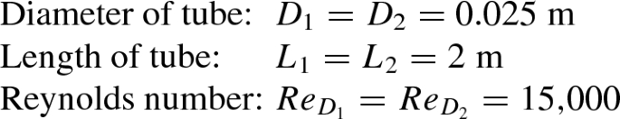
A highly viscous oil flows under a head of 0.5 m of water through two tubes that are arranged in parallel. The first tube has a diameter of 3 mm and the second has a diameter of 4 mm. Both tubes are 1 m long. Determine the volume flow rates in the two tubes. The viscosity of oil may be taken as 3 times the viscosity of water and the relative density of oil is 0.8. Take water properties at $30\,^\circ \mathrm{C}$.

Solution:

Step 1:

Water properties at $30\,^\circ \mathrm{C}$ are taken from table of properties of water. They are

$$\begin{aligned} \rho _w= 995.7\;\mathrm{kg}/\mathrm{m}^3,\;\mu _w=7.97\times 10^{-4}\;\mathrm{kg}/\mathrm{m}\;\mathrm{s} \end{aligned}$$

The flowing fluid is oil with the following properties:

Step 2:

The given data is written down as below

Step 3:

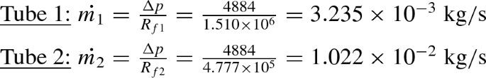
Available pressure drop is given to be equal to a head of water of $h=0.5$ m. The corresponding pressure drop is given by

$$\begin{aligned} \Delta p=\rho _w gh=995.7\times 9.81\times 0.5 =4884\;\mathrm{Pa} \end{aligned}$$

where we have used the standard value for the acceleration due to gravity of $g=9.81$ m/s$^2$. We shall assume that the flow through both tubes is laminar. Of course we shall verify it later on.

Step 4:

The flow resistance of the tubes may be obtained using Eq. 12.64.

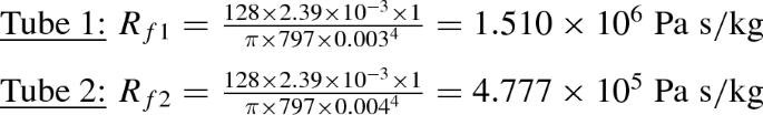
Step 5:

Using the definition of flow resistance, the mass flow rates in the two tubes may be calculated now.

The corresponding oil velocities in the two cases are given by

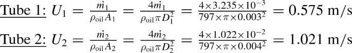
Step 6:

We now verify whether the flow is laminar in the two cases. This is done by making sure that the larger of the two Reynolds numbers is less than 2300. The Reynolds number in the case of 4 mm tube is the larger of the two and is

$$\begin{aligned} Re_{D_2}=\frac{\rho _\mathrm{oil}U_2D_2}{\mu _\mathrm{oil}} =\frac{797\times 1.021\times 0.004}{2.39\times 10^{-3}} =1361 \end{aligned}$$

The flow is indeed laminar and the use of laminar flow resistance formula is justified.

Step 7:

The volume flow rates are obtained now.

12.4 Laminar Heat Transfer in Tube Flow

Heat transfer to or from a fluid flowing in a tube is of great importance since this configuration is very common in heat transfer devices such as heat exchangers. Even though laminar flow is not very common, the analysis of laminar flow provides an opportunity to learn about convection in internal flow using simple mathematics. Two boundary conditions that are easily achieved in practice are the constant heat flux and the constant wall temperature conditions. The former is obtained by electrical heating of a highly conducting tube and the latter by having condensing or evaporating fluid in contact with the outside of the tube wall.

12.4.1 Bulk Mean Temperature

Recall from the discussion in Sect. 12.3.4 where the mean velocity for flow in a tube was defined. The fluid flowing at the mean velocity transports a constant amount of fluid per unit time along the tube. In a heat transfer application, we would be interested in determining the rate at which enthalpy is transported across any cross section of the tube. This is easily done by introducing the so called bulk mean temperature (also known as the mixing cup temperature). The rate at which enthalpy $\dot{H}(z)$ is transported across any section of the tube is obtained by the following integral:

$$\begin{aligned} \dot{H}(z)=\int \limits _0^R C_pT(r,z)d\dot{m} \end{aligned}$$

where $d\dot{m}$ is the mass flow rate through an elemental area given by $2\pi rdr$ and $C_pT(r,z)$ is the magnitude of the enthalpy of the fluid entering the elemental area. The elemental mass flow rate itself is obtained as the product of density, area, and the velocity as

$$\begin{aligned} d\dot{m}=\rho \times 2\pi rdr\times u_z(r,z) \end{aligned}$$

Combining these we get

$$\begin{aligned} \dot{H}(z)=\int \limits _0^R 2\rho \pi ru_z(r,z)C_pT(r,z)dr \end{aligned}$$

(12.67)

We shall equate the rate of enthalpy crossing the tube section by introducing the mean velocity introduced earlier and the bulk mean temperature $T_B(z)$ such that $\dot{H}(z)=\dot{m}C_pT_B(z)=(\pi R^2\rho U)C_pT_B(z)$. Note that this is the product of the mass flow rate across the section and the mean value of enthalpy of the entering fluid. Thus, we get for a constant property fluid

$$\begin{aligned} \begin{aligned} \left( \pi R^2\rho U\right) \left( C_pT_B(z)\right) =\int \limits _0^R 2\rho \pi r u_z(r,z)C_pT(r,z)dr\\ \text {or}\boxed {T_B(z)=\frac{2}{\pi R^2U}\int \limits _0^R u_z(r,z)T(r,z)dr} &\end{aligned} \end{aligned}$$

(12.68)

Note that the bulk mean temperature as defined above is valid at any z along the flow and may, in fact, vary with z. However, U is independent of z because of mass conservation, even though $u_z$ may be a function of r and z. In what follows we shall be interested in applying the above to the fully developed region where $u_z$ will be a function of r alone.

12.4.2 Variation of the Bulk Mean Temperature

The bulk mean temperature varies with z, and this variation depends on the condition applicable at the tube wall. In most practical applications the tube wall is thin, and hence it is customary to neglect axial heat conduction in the tube wall, i.e., heat conduction along the z-direction. Hence, heat transfer across the tube wall is assumed to be radial. This heat transfer may be subject to a very small temperature variation across the tube wall if it is thin and made of a material with a high thermal conductivity. Hence, it is possible to make a simple analysis assuming that heat transfer to the fluid or away from the fluid takes place radially and is specified at the fluid–solid interface.

The analysis may be made using the control volume shown in Fig. 12.8. The control volume is taken in the form of a short cylinder of length $\Delta z$ and of radius R, equal to the inner radius of the tube.

Fig. 12.8

Control volume for heat transfer analysis

Heat balance may be made for the control volume as follows:

$$\begin{aligned} \left[ \begin{array}{c} \text {Heat convected}\\ \text {across left boundary}\\ \end{array}\right] +\left[ \begin{array}{c} \text {Heat transfer entering}\\ \text {at tube wall}\\ \end{array}\right] =\left[ \begin{array}{c} \text {Heat convected}\\ \text {across right boundary}\\ \end{array}\right] \end{aligned}$$

The heat transfer by convection entering through the left boundary is obtained by the use of the bulk mean temperature as $\rho \pi R^2UC_pT_B(z)$. The heat transfer by convection leaving through the right boundary may be written as $\rho \pi R^2UC_pT_B(z+\Delta z)=\rho \pi R^2UC_p\left[ T_B(z)+\frac{dT_B}{dz}\Delta z\right]$. We have made use of the Taylor expansion and retained only the first-order term. The heat transfer entering at the tube wall is given by $2\pi Rq_w\Delta z$. Introducing these in the heat balance equation and simplifying, we get

$$\begin{aligned} \boxed {\frac{dT_B}{dz}=\frac{2q_w}{\rho UC_pR}} \end{aligned}$$

(12.69)

The above equation is general in that it applies to any variation of $q_w$ with z. In the special case in which $q_w$ is constant, the bulk mean temperature increases (or decreases if $q_w$ is negative, i.e., heat is lost from the fluid element to the tube wall) linearly with z.

12.4.3 Tube Flow with Uniform Wall Heat Flux

Consider tube flow with heat transfer as indicated in Fig. 12.9. The fluid enters with a uniform temperature $T_0$ as indicated. The wall is subjected to a constant heat flux $q_w$. There is a thermal entry length $L_\mathrm{dev}'$  over which the temperature distribution develops just as the flow development would take place over an entry length $L_\mathrm{dev}$ discussed earlier. For laminar flow, the entry length is given by $L_\mathrm{dev}'/D = 0.05 Re_D Pr=0.05Pe$ where the Reynolds number Prandtl number product has been represented as Pe, the Peclet number.⁵ For $z >L_\mathrm{dev}'$ the temperature is fully developed, and for $q_w = \text {constant}$, both $T_w$ and $T_B$ increase linearly at the same rate, keeping a constant difference between the two. Here, $T_B$ is the bulk mean temperature of the fluid, as defined earlier through Eq. 12.68.

Fig. 12.9

Tube flow with constant heat flux at its surface

12.4.4 Fully Developed Temperature with Uniform Wall Heat Flux

The idea of fully developed temperature profile is analogous to the fully developed velocity profile considered earlier. We look for a suitably defined non-dimensional temperature profile that is a function of r only, being thus independent of z. This is in spite of the fact that the temperature of the fluid varies with both r and z. Consider the non-dimensional temperature ratio given by

$$\begin{aligned} \theta (r)=\frac{T(r,z)-T_w(z)}{T_B(z)-T_w(z)} \end{aligned}$$

(12.70)

where $T_w(z)$ stands for the wall temperature and $T_B(z)$ is the bulk mean temperature of the fluid. As indicated in Eq. 12.70, $\theta$ is a function of only r and hence $\frac{\partial \theta }{\partial z}\equiv 0$. This requires that

$$\begin{aligned} \frac{\partial \theta }{\partial z} =\frac{\dfrac{\partial T(r,z)}{\partial z}-\dfrac{d T_w(z)}{d z}}{T_B(z)-T_w(z)}-\frac{T(r,z)-T_w(z)}{\left[ T_B(z)-T_w(z)\right] ^2} \left( \frac{dT_B(z)}{dz}-\frac{dT_w(z)}{dz}\right) =0 \end{aligned}$$

(12.71)

which may be rewritten, by removing the common factor $T_B(z)-T_w(z)$ in the denominator, as

$$\begin{aligned}{}[T_B(z)-T_w(z)]\frac{\partial \theta }{\partial z} =\left[ \frac{\partial T(r,z)}{\partial z}-\frac{d T_w(z)}{d z}\right] -\theta (r) \left[ \frac{dT_B(z)}{dz}-\frac{dT_w(z)}{dz}\right] =0 \end{aligned}$$

(12.72)

In the present case of uniform tube wall flux, the above expression will hold only if

$$\begin{aligned} \frac{\partial T(r,z)}{\partial z}=\frac{d T_w(z)}{d z} =\frac{dT_B(z)}{dz} \end{aligned}$$

(12.73)

This may be combined with Eq. 12.69 to get

$$\begin{aligned} \frac{\partial T(r,z)}{\partial z}=\frac{d T_w(z)}{d z} =\frac{dT_B(z)}{dz}=\frac{2q_w}{\rho UC_pR} \end{aligned}$$

(12.74)

where the wall heat flux $q_w$ is a constant independent of z. Hence, the axial temperature gradient $\frac{\partial T(r,z)}{\partial z}$ is a constant, and hence the second derivative of T(r, z) with respect to z is zero. This means that the axial heat conduction does not change with z and hence the axial diffusion term drops off.

Governing equation

The governing equation may be developed either from the energy equation in cylindrical coordinates (see Appendix H) or from first principles as is done here. Consider energy balance over an annular element as shown in Fig. 12.10.

Since conduction flux along the axis does not change with z, net convection crossing the control volume in the axial direction is balanced by net conduction in the radial direction. With this in mind, the fluxes crossing the control volume are as shown in the figure. Energy balance may be spelt out in words as follows:

$$\begin{aligned} \left[ \begin{array}{c} \text {Conduction }\\ \text {leaving at }\\ \text {outer boundary}\\ \end{array}\right] -\left[ \begin{array}{c} \text {Conduction }\\ \text {entering at inner}\\ \text {boundary}\\ \end{array}\right] =\left[ \begin{array}{c} \text {Convection }\\ \text {leaving across }\\ \text {right boundary}\\ \end{array}\right] -\left[ \begin{array}{c} \text {Convection }\\ \text {entering across}\\ \text {left boundary}\\ \end{array}\right] \end{aligned}$$

As usual we use Taylor expansion retaining first-order terms to write, after simplification, the following governing equation.

Fig. 12.10

Annular control volume for developing the governing equation

$$\begin{aligned} k\frac{\partial }{\partial r}\left( r\frac{\partial T}{\partial r}\right) =\rho u_zC_pr\frac{\partial T}{\partial z} \end{aligned}$$

(12.75)

We shall assume now that the velocity profile is given by the fully developed profile (see Eq. 12.40). We also use the variation of temperature along z given by Eqs. 12.69 and 12.74 to write the governing equation as

$$\begin{aligned} \frac{\partial }{\partial r}\left( r\frac{\partial T}{\partial r}\right) =\frac{4q_wr}{kR}\left[ 1-\left( \frac{r}{R}\right) ^2\right] \end{aligned}$$

(12.76)

We may recast this equation in terms of the non-dimensional temperature $\theta (r)$ introduced through Eq. 12.70 as

$$\begin{aligned} \boxed {\frac{d}{dr}\left( r\frac{d\theta }{dr}\right) =\frac{4q_wr}{kR\{T_B(z)-T_w(z)\}}\left[ 1-\left\{ \frac{r}{R}\right\} ^2\right] } \end{aligned}$$

(12.77)

where the partial derivatives have become total derivatives since $\theta$ is independent of z. Note also that $T_B(z)-T_w(z)$ in the denominator should be independent of z since $q_w$ is independent of z. The ratio of wall heat flux to driving temperature difference defines the convection heat transfer coefficient h which is a constant independent of z. We define the Nusselt number $Nu_H$ as the Nusselt number in the fully developed region with constant flux boundary condition through the relation

$$\begin{aligned} Nu_H=\frac{q_wD}{k\left\{ T_w(z)-T_B(z)\right\} } \end{aligned}$$

(12.78)

such that the governing equation may be recast as

$$\begin{aligned} \frac{d}{d\zeta }\left( \zeta \frac{d\theta }{d\zeta }\right) =-2Nu_H\zeta (1-\zeta ^2) \end{aligned}$$

(12.79)

The accompanying boundary conditions are specified as

$$\begin{aligned} \theta \;\text {is finite at}\;\zeta =0;\;\text {and}\;\frac{q_w}{T_B(z)-T_w(z)}-k\frac{d\theta }{dr} = 0\; \text {at}\;r=R \end{aligned}$$

(12.80)

in dimensional form. The boundary condition at tube wall is a statement of the fact that the heat flux is continuous across the boundary. This may be rewritten in non-dimensional form, using the Nusselt number defined above as

$$\begin{aligned} \frac{d\theta }{d\zeta }+\frac{Nu_H}{2}=0\; \text {at}\;\zeta =1 \end{aligned}$$

(12.81)

Solution

Equation 12.76 is integrated once with respect to $\zeta$ to get

$$\begin{aligned} \frac{d\theta }{d\zeta }=-2Nu_H\left( \frac{\zeta }{2}-\frac{\zeta ^3}{4}\right) +\frac{C_1}{\zeta } \end{aligned}$$

where $C_1$ is a constant of integration. The boundary condition at $\zeta =0$ requires that we choose $C_1$ as 0. The resulting equation is integrated once more with respect to $\zeta$ to get

$$\begin{aligned} \theta =-2Nu_H\left( \frac{\zeta ^2}{4}-\frac{\zeta ^4}{16}\right) +C_2 \end{aligned}$$

(12.82)

where $C_2$ is a second constant of integration. It is seen that the constant of integration, in fact, represents the non-dimensional temperature $\theta _0$ at the axis of the tube, that is not known as of now. Thus, we write Eq. 12.82 as

(12.83)

The boundary condition at the tube wall is not available to us since it has been implicitly used in deriving Eq. 12.69 by overall energy balance. Consider the following integral:

$$\begin{aligned} I_n=\int \limits _0^R u_z(r)\phi (r) r dr= R^2\int \limits _0^1 2U(1-\zeta ^2)\phi (\zeta )\zeta d\zeta \end{aligned}$$

Using the non-dimensional temperature profile given by Eq. 12.83, the above integral is written as

$$\begin{aligned} \begin{aligned} I_n=-4UR^2Nu_H\int \limits _0^1 (1-\zeta ^2)\left( \frac{\zeta ^2}{4}-\frac{\zeta ^4}{16}\right) \zeta d\zeta = -UR^2Nu_H\int _0^1\left[ \zeta ^3- \frac{5\zeta ^5}{4}+\frac{\zeta ^7}{4}\right] d\zeta \\ =-UR^2Nu_H\left[ \frac{\zeta ^4}{4}- \left. \frac{5\zeta ^6}{24}+\frac{\zeta ^8}{32}\right] \right| _{\zeta =0}^1=-UR^2Nu_H\left( \frac{7}{96}\right) &\end{aligned} \end{aligned}$$

(12.84)

Consider also the integral $I_d=\int \limits _0^Ru_z(r)r dr$. We may easily obtain this integral as

$$\begin{aligned} I_d=2UR^2\int \limits _0^1(\zeta -\zeta ^3)d\zeta =\frac{UR^2}{2} \end{aligned}$$

(12.85)

Finally, by division, we get

$$\begin{aligned} \frac{I_n}{I_d}=-\frac{7}{48}Nu_H \end{aligned}$$

(12.86)

We recognize this to represent $\theta _B-\theta _0$. We may obtain from this the difference $\theta _B-\theta _w$ as

$$\begin{aligned} \theta _B-\theta _w=1=[\theta _B-\theta _0]-[\theta _w-\theta _0] \end{aligned}$$

where the relation $\theta _B-\theta _w=1$ follows from the definition of the non-dimensional temperatures. The second term on the right-hand side is obtained by evaluating Eq. 12.83 at $\zeta =1$ as

$$\begin{aligned} \theta -\theta _0=-2Nu_H\left( \frac{1}{4}-\frac{1}{16}\right) =-\frac{3}{8}Nu_H \end{aligned}$$

(12.87)

With these, we get

$$\begin{aligned} \theta _B-\theta _w=1=-\frac{7}{48}Nu_H+\frac{3}{8}Nu_H \end{aligned}$$

or

$$\begin{aligned} \boxed { Nu_H=\frac{48}{11}=4.364} \end{aligned}$$

(12.88)

Hence, the Nusselt number is a constant equal to 4.364 (the heat transfer coefficient is also a constant) in fully developed tube flow with constant wall flux. Obviously, the Nusselt number is not what is important when the wall heat flux is specified or known. The above equation is useful in determining the difference between the wall and bulk fluid temperature as

$$\begin{aligned} T_w(z)-T_B(z)=\frac{11}{48}\frac{q_wD}{k} \end{aligned}$$

(12.89)

The non-dimensional temperature variation across the tube may now be represented using Eqs. 12.83 and 12.87 as

$$\begin{aligned} \theta _w-\theta =(\theta _w-\theta _0)-(\theta -\theta _0) =-2Nu_H\left( \frac{\zeta ^2}{4}-\frac{\zeta ^4}{16}\right) +\frac{3}{8}Nu_H \end{aligned}$$

Using the known value of $Nu_H$, the above becomes

$$\begin{aligned} \boxed {\theta _w-\theta =\frac{24}{11}\left\{ \frac{3}{4}- \zeta ^2+\frac{\zeta ^4}{4}\right\} } \end{aligned}$$

(12.90)

12.4.5 Tube Flow with Constant Wall Temperature

As mentioned earlier the constant wall temperature case is typical of what happens when the outer wall of the tube is in contact with a fluid undergoing phase change, such as in a condenser of a steam power plant. The tube side fluid (i.e., the fluid that flows inside the tube) is usually water. The flow velocity and the tube diameter are such that the flow in the tube is invariably turbulent. However, it is instructive to look at the laminar flow case since fundamental ideas involved in heat transfer are the same in the laminar case also. Schematic of tube flow with constant wall temperature is as shown in Fig. 12.11. The temperature field undergoes a development over an entry length $L_\mathrm{dev}'$. The temperature in the core remains constant at $T_0$ till $z=L_\mathrm{dev}'$. Thereafter the thermal boundary layer fills the entire tube. The bulk temperature varies as indicated graphically at the bottom of Fig. 12.11. Assuming that the fluid in the tube is getting heated, $T_B$ will continually increase but the rate of heat transfer continuously reduces since the driving temperature difference continuously decreases with z. We shall see later that the temperature difference reduces exponentially with z when the heat transfer coefficient is constant.

Fig. 12.11

Tube flow with constant wall temperature

12.4.6 Fully Developed Tube Flow with Constant Wall Temperature

Let us see what happens in the fully developed temperature region. We go back to Eq. 12.72 and notice that the fully developed condition holds only if

$$\begin{aligned} \theta (r)\frac{dT_B}{dz}=\frac{\partial T(r,z)}{\partial z} \end{aligned}$$

(12.91)

since $\frac{dT_w}{dz}=0$.

We shall look at this condition after deriving the appropriate equation that governs the temperature field.

Governing equation

We derive the governing equation starting with the energy Eq. H.38 in cylindrical coordinates given in Appendix H. Since the flow is steady $\frac{\partial }{\partial t}\equiv 0$. The flow velocity component along the axis of the tube alone is non-zero, and hence, the convective term consists of only the term $u_z\frac{\partial T(r,z)}{\partial z}$. The diffusion terms (terms appearing in the energy equation that account for conduction in the fluid) will involve both derivatives with respect to r and z and the governing equation becomes

$$\begin{aligned} u_z\frac{\partial T}{\partial z}=\alpha \Big [\frac{1}{r} \frac{\partial }{\partial r}\Big (r\frac{\partial T}{\partial r}\Big ) +\frac{\partial ^2T}{\partial z^2}\Big ] \end{aligned}$$

(12.92)

On the right-hand side of Eq. 12.92, we have the axial diffusion represented by the second derivative of T with respect to z. In the case of tube flow with constant wall heat flux this term dropped off since $\frac{\partial T}{\partial z}$ was a constant. In the present case, we shall assume that this axial conduction term is negligibly small when compared to the radial conduction term represented by the derivative with respect to r. We justify this assumption based on estimates for the derivatives. We may approximate the derivatives by differences and hence

$$\begin{aligned} \frac{\partial T}{\partial z}\sim \frac{T_{B,o}-T_{B,i}}{L}\;\text {and}\;\frac{\partial ^2 T}{\partial z^2}\sim \frac{T_{B,o}-T_{B,i}}{L^2} \end{aligned}$$

where the inlet and outlet bulk temperatures are used to define the characteristic temperature difference, and the length of tube to define the characteristic length. However, for the derivatives in the r direction, we use the difference between the mean of the bulk mean temperatures $T_{B,\,\mathrm{mean}}=\frac{T_{B,o}+T_{B,i}}{2}$ and wall temperature as the characteristic temperature difference and tube radius R as the characteristic length to write

$$\begin{aligned} \frac{1}{r} \frac{\partial }{\partial r}\Big (r\frac{\partial T}{\partial r}\Big ) \sim \frac{T_{B,\,\mathrm{mean}}-T_w}{R^2} \end{aligned}$$

In applications, invariably the temperature difference of the fluid between the entry and exit is smaller than that between the fluid and the wall. For example, the bulk temperature difference may be $15\,^\circ \mathrm{C}$ while the temperature difference between the fluid and the wall may be $50\,^\circ \mathrm{C}$. Also the length of the tube L is normally much larger than the radius R of the tube. For example, with a tube Reynolds number of 1000 fully developed conditions are obtained with $\frac{L}{D}>\frac{L_\mathrm{dev}'}{D}=0.05\times 1000\times 5=250$ or $\frac{L}{R}>500$ where the Prandtl number has been assumed to have a value of 5, typical of water. With $R=0.005$ m, the corresponding L is about 2.5 m. The axial and radial diffusion terms are typically given by

$$\begin{aligned} \text {Axial diffusion term:}&\frac{T_{B,o}-T_{B,i}}{L^2}\approx \frac{15}{2.5^2}=2.4\;^\circ \mathrm{C}/\mathrm{m}^2 \\ \text {Radial diffusion term:}&\frac{50}{0.005^2} =2\times 10^6\;^\circ \mathrm{C}/\mathrm{m}^2 \end{aligned}$$

It is thus clear that the axial diffusion term is much smaller than the radial diffusion term, thus justifying the assumption suggested above. Hence, we approximate the governing equation, neglecting axial conduction, as

$$\begin{aligned} u_z\frac{\partial T}{\partial z}\approx \alpha \frac{1}{r} \frac{\partial }{\partial r}\left( r\frac{\partial T}{\partial r}\right) \end{aligned}$$

(12.93)

Further, we shall assume that $u_z$ is given by the fully developed velocity profile specified by Eq. 12.40. Additionally, making use of the fully developed temperature condition Eq. 12.91 and $\theta$ defined by Eq. 12.70, we simplify the governing equation to

$$\begin{aligned} \alpha \frac{1}{r} \frac{\partial }{\partial r}\left( r\frac{\partial T}{\partial r}\right) =2U\left[ 1-\left( \frac{r}{R}\right) ^2\right] \theta \frac{dT_B}{dz} \end{aligned}$$

(12.94)

By definition, the fully developed temperature profile is a function of r alone and hence

where Eq. 12.70 has been made use of. Also the radial diffusion term takes the form

$$\begin{aligned} \alpha \frac{1}{r} \frac{\partial }{\partial r}\left( r\frac{\partial T}{\partial r}\right) =(T_B-T_w)\alpha \frac{1}{r}\frac{d}{dr}\left( r\frac{d\theta }{dr}\right) \end{aligned}$$

Thus, the governing equation takes the form of an ordinary differential equation given by

$$\begin{aligned} \frac{1}{r} \frac{d}{dr}\left( r\frac{d\theta }{dr}\right) =2\frac{U}{\alpha }\left[ 1-\left( \frac{r}{R}\right) ^2\right] \frac{\dfrac{dT_B}{dz}}{(T_B-T_w)}\theta \end{aligned}$$

(12.95)

We immediately see that $\frac{\dfrac{dT_B}{dz}}{(T_B-T_w)}$ should be independent of z. This is, in fact, the real import of the fully developed temperature profile. Using the relationship between wall heat flux and the driving temperature difference given by Eq. 12.69, we have

$$\begin{aligned} \frac{U}{\alpha }\frac{\dfrac{dT_B}{dz}}{(T_B-T_w)}=-\frac{2q_w(z)}{kR(T_w-T_B)} =-\frac{Nu_T}{R^2} \end{aligned}$$

(12.96)

where $Nu_T$ is the constant Nusselt number in the fully developed region in the constant wall temperature case. Using the non-dimensional variable $\zeta =\frac{r}{R}$, the governing equation takes the form

$$\begin{aligned} \boxed {\frac{1}{\zeta } \frac{d}{d\zeta }\left( \zeta \frac{d\theta }{d\zeta }\right) =\frac{d^2\theta }{d\zeta ^2}+\frac{1}{\zeta }\frac{d\theta }{d\zeta } =-2Nu_T(1-\zeta ^2)\theta } \end{aligned}$$

(12.97)

This equation is to be solved with the boundary conditions given by

$$\begin{aligned} \theta \;\text {is finite at}\;\zeta =0,\;\text {and}\;\theta =0\;\text {at}\;\zeta =1 \end{aligned}$$

(12.98)

Solution

Since the governing equation is an ordinary differential equation with variable coefficients, the solution may be obtained by using an infinite series to represent the temperature field.⁶ The solution that is finite at the origin will have only positive powers of $\zeta$ in the series. Since the parameter $Nu_H$ is not known, the solution will involve this as a parameter. The boundary condition at the tube wall will determine $Nu_H$ as we shall soon see. Since the solution is axisymmetric, only even powers of $\zeta$ will occur in the series solution. Hence, let the solution be represented by the series given by

$$\begin{aligned} \theta =\sum _{n=0}^{\infty }C_{2n}\zeta ^{2n} \end{aligned}$$

(12.99)

On substitution in Eq. 12.97, using term by term differentiation, collecting terms containing same powers of $\zeta$, we get the following:

$$\begin{aligned} \nonumber \zeta ^{-2}:&C_0\times 0\;\text {Hence}\;C_0\ne 0 \\ \nonumber \zeta ^0:&4C_2+\lambda ^2C_0\\ \nonumber \text {Hence}\;&C_2=-\frac{\lambda ^2}{4}C_0 \\ \nonumber&\cdots&\\ \nonumber \zeta ^{2n}:&(2n)^2 C_{2n}-\lambda ^2\left( C_{2n-4}-C_{2n-2}\right) \\ \text {Hence}\;&C_{2n}=-\frac{\lambda ^2}{(2n)^2}\left( C_{2n-4}-C_{2n-2}\right) \end{aligned}$$

(12.100)

where, for convenience, $\lambda ^2$ stands for $2Nu_T$. Hence, the solution may be written as

$$\begin{aligned} \theta =C_0\left[ 1-\frac{\lambda ^2}{4}\zeta ^2+ \frac{\lambda ^2}{16}\left( 1+\frac{\lambda ^2}{4}\right) \zeta ^4-\frac{\lambda ^2}{36}\left\{ \frac{\lambda ^2}{4}+\frac{\lambda ^2}{16}\left( 1+\frac{\lambda ^2}{4}\right) \right\} \zeta ^6-+\cdots \right] \end{aligned}$$

(12.101)

Note that both $C_0$ and $\lambda$ are unknown as of now. The non-dimensional temperature has to vanish at the tube wall, and hence, the series given by Eq. 12.101 should vanish at $\zeta =1$. Luckily for us the series converges rapidly, and it is necessary to take only 10 terms. Since $C_0$ is non-zero, the sum of terms within the braces have to vanish. By trial, it may be verified that the sum vanishes for $\lambda ^2=7.313588$, and hence the value of the Nusselt number is given by

$$\begin{aligned} \boxed {Nu_T=\frac{\lambda ^2}{2}=\frac{7.313588}{2} =3.656794\approx 3.657} \end{aligned}$$

(12.102)

The value of the unknown constant $C_0$ may be determined by using the heat flux continuity condition at $\zeta =1$. This requires that (Eq. 12.81 with $Nu_H$ replaced by $Nu_T$)

$$\begin{aligned} \frac{d\theta }{d\zeta }\Big |_{\zeta =1}=-\frac{Nu_T}{2} =-\frac{3.656794}{2}=-1.828397 \end{aligned}$$

(12.103)

The derivative required may be calculated by term by term differentiation of series given by Eq. 12.101 and inserting $\zeta =1$ to get

$$\begin{aligned} \frac{d\theta }{d\zeta }=C_0\times (-1.01428)=-1.828397 \;\text {or}\;C_0=1.802652 \end{aligned}$$

(12.104)

The fully developed temperature (constant wall heat flux and constant wall temperature cases) and velocity profiles are shown in Fig. 12.12. While the velocity profile is quadratic in $\zeta =\frac{r}{R}$ the temperature profile is a quartic in $\zeta$, in the case of constant heat flux case (identified as $\theta _H$) while it is given by an infinite series in the case of the constant wall temperature case (identified as $\theta _T$). The maximum non-dimensional temperature difference occurs between the wall and the fluid at the tube axis, in both cases. The maximum velocity occurs along the tube axis.

Fig. 12.12

Fully developed velocity and temperature profiles

Example 12.5

Ethylene glycol is flowing in a $D=6$ mm diameter thin-walled copper tube heated electrically such that the wall heat flux is $q_w=1000$ W/m$^2$. At a certain section, glycol has a bulk mean temperature of $70\,^\circ \mathrm{C}$. The volume flow rate of glycol has been measured to be $\dot{V}=15$ ml/s. Determine the wall temperature at this location. Also determine rate of change of the bulk temperature of glycol with axial distance.

Glycol properties may be taken as constant and are specified as below Density $\rho = 1109$ kg/m$^3$, Dynamic viscosity $\mu = 0.0144$ kg/m s, Thermal conductivity $k = 0.2814$ W/m $^\circ \mathrm{C}$, and Prandtl number $Pr = 124.4$.

Solution:

Step 1:

Flow area is calculated as

$$\begin{aligned} A=\frac{\pi D^2}{4}=\frac{\pi \times 0.006^2}{4} =2.82743\times 10^{-5}\;\mathrm{m}^2 \end{aligned}$$

Step 2:

The mean velocity of glycol in the tube is then obtained as

$$\begin{aligned} U=\frac{\dot{V}}{A}=\frac{15\times 10^{-6}}{2.82743\times 10^{-5}} =0.531\;\mathrm{m}/\mathrm{s} \end{aligned}$$

Step 3:

The flow Reynolds number is determined as

$$\begin{aligned} Re_D=\frac{\rho UD}{\mu }=\frac{1109\times 0.531\times 0.006}{0.0144} =245 \end{aligned}$$

Since the Reynolds number is less than 2300, the flow is laminar. The results of preceding analysis of fully developed tube flow with constant wall heat flux are used to get the desired results.

Step 4:

The Nusselt number has the fully developed value of $Nu_H=\frac{48}{11}=4.364$. Using the definition of Nusselt number, the corresponding heat transfer coefficient may be obtained as

$$\begin{aligned} h=\frac{Nu_Hk}{D}=\frac{4.364\times 0.2814}{0.006} =204.65\;\mathrm{W}/\mathrm{m}^{2\;\circ }\mathrm{C} \end{aligned}$$

Step 5:

The driving temperature difference at any z in the fully developed region is

$$\begin{aligned} T_w-T_B=\frac{q_w}{h} =\frac{1000}{204.65}=4.89\,^\circ \mathrm{C} \end{aligned}$$

Step 6:

It is given that the bulk temperature at a certain location along the tube is $T_B=70\;^\circ \mathrm{C}$. Hence, the corresponding wall temperature is

$$\begin{aligned} T_w=70+4.89=74.89\,^\circ \mathrm{C} \end{aligned}$$

Step 7:

The specific heat of glycol may be obtained by making use of the thermo-physical properties specified in the problem as

$$\begin{aligned} C_p=\frac{Pr\cdot k}{\mu } =\frac{124.4\times 0.2814}{0.0144} =2431\;\mathrm{J}/\mathrm{kg}\,^\circ \mathrm{C} \end{aligned}$$

Step 8:

To determine the axial temperature gradient, we make use of Eq. 12.74 to get

$$\begin{aligned} \frac{dT_B}{dz}=\frac{2q_w}{\rho UC_pR} =\frac{2\times 1000}{1109\times 0.531\times 2431\times 0.003} =0.47\,^\circ \mathrm{C}/\mathrm{m} \end{aligned}$$

Example 12.6

Air is heated by passing it through a copper tube of $2.5\;mm$ ID that is steam jacketed with steam at $100\,^\circ \mathrm{C}$. The properties of air may be taken at a mean temperature of $40\,^\circ \mathrm{C}$. The steam side heat transfer coefficient is extremely large, and hence, the wall of the tube may be assumed to be essentially at the steam temperature. At a certain location along the tube, both flow and temperature are fully developed. Determine the axial gradient of the bulk mean temperature at this location if the bulk mean temperature is $60\,^\circ \mathrm{C}$ when the mass flow of rate of air is $0.05\;\mathrm{g}/\mathrm{s}$.

Solution:

Air properties at $40\,^\circ \mathrm{C}$ are

Other data specified in the problem are

Air velocity in the tube may be calculated as

$$\begin{aligned} U=\frac{\dot{m}}{\rho A} =\frac{4\dot{m}}{\rho \pi D^2}=\frac{4\times 5\times 10^{-5}}{1.1169\times \pi \times 0.0025^2}=9.12\;\mathrm{m}/\mathrm{s} \end{aligned}$$

Tube Reynolds number is then given by

$$\begin{aligned} Re_D=\frac{\rho UD}{\mu }=\frac{1.1169\times 9.12\times 0.0025}{1.91\times 10^{-5}} =1340 \end{aligned}$$

Since the Reynolds number is less than 2300, the flow is laminar. Hence, we may use the results of analysis presented previously to obtain the axial temperature gradient. In particular, we make use of Eq. 12.96 to get

$$\begin{aligned} \frac{dT_B}{dz}=-\frac{Nu_T\alpha (T_B-T_z)}{UR^2} \end{aligned}$$

The thermal diffusivity $\alpha$ appearing in the above is obtained as

$$\begin{aligned} \alpha =\frac{k}{\rho C_p} =\frac{0.0274}{1.1169\times 1005}=2.441\times 10^{-5}\;\mathrm{m}^2/\mathrm{s} \end{aligned}$$

Under the fully developed condition the Nusselt number $Nu_T$ is equal to 3.657. Hence, the axial gradient of the bulk mean temperature may be obtained as

$$\begin{aligned} \frac{dT_B}{dz}=-\frac{3.657\times 2.441\times 10^{-5}(60-100)}{9.12\times 0.00125^2}=250.58\;^\circ \mathrm{C}/\mathrm{m} \end{aligned}$$

12.5 Laminar Fully Developed Flow and Heat Transfer in Non-circular Tubes and Ducts

12.5.1 Introduction

Tubes and ducts of non-circular cross section are used in many heat transfer applications. The concept of flow and temperature development applies equally to these cases. The Reynolds and Nusselt numbers are based on suitably defined characteristic lengths. The characteristic length is also known as the hydraulic diameter in the case of the flow problem and the energy diameter in the case of the heat transfer problem. These two may or may not be the same, for a given duct or tube of non-circular cross section.

Fig. 12.13

Non-circular duct nomenclature—the hydraulic diameter

We have earlier seen how the friction factor for a parallel plate channel is expressed using the hydraulic diameter as the characteristic length scale. Figure 12.13 shows how the hydraulic diameter $D_H$ is defined, for the case of a duct or tube of any cross section. For the flow problem, the hydraulic diameter uses the so-called wetted perimeter $P_w$—the perimeter over which there is contact between the flowing fluid and the solid wall—where viscous shear is manifest. In the case of a tube of circular diameter, the wetted perimeter is obviously the circumference of the circle representing the cross section of the tube. The flow area is the cross-sectional area $A_c$ of the tube. In case of an annulus—the flow takes place in the region between an inner and outer tube—the wetted perimeter is the sum of the circumferences of the outer surface of the inner tube and the inner surface of the outer tube. The flow area is the area of the annulus.

The hydraulic diameter $D_H$ is defined by the following relation:

$$\begin{aligned} D_H=\frac{4A_c}{P_w} \end{aligned}$$

(12.105)

In the case of a circular cross-sectional tube, the hydraulic and actual diameter are the same. In the case of an annulus with inner diameter $D_i$ and outer diameter $D_o$, we have

$$\begin{aligned} P_w=\pi \left( D_i+D_o\right) ;\;\; A_c=\frac{\pi \left( D_o^2-D_i^2\right) }{4};\;\; D_H =\frac{4\dfrac{\pi \left( D_o^2-D_i^2\right) }{4}}{\pi \left( D_i+D_o\right) } =\left( D_o-D_i\right) \end{aligned}$$

12.5.2 Parallel Plate Channel with Asymmetric Heating

The fully developed flow in this geometry has been considered in Sect. 12.3.5. We shall now consider the case of fully developed temperature problem. Detailed solution is worked out for the case where the top wall is subject to uniform heat flux $q_w$ while the bottom wall is adiabatic (refer Fig. 12.7). The energy equation may be written for the present case starting from the cartesian form of equation given in Appendix H. This is left as an exercise to the reader. The appropriate equation in non-dimensional form is

$$\begin{aligned} \frac{d^2\theta }{d\zeta ^2}=-\frac{3}{16}Nu_H(1-\zeta ^2) \end{aligned}$$

(12.106)

where the velocity field has been replaced using the fully developed profile given by

$$\begin{aligned} \frac{u}{U}=1-\zeta ^2 \end{aligned}$$

$Nu_H$ in this case is defined as $\frac{4bq_w}{k(T_w-T_B)}$ where $T_w$ is the top (heated) wall temperature and 4b is the hydraulic diameter. The boundary conditions are specified as

$$\begin{aligned} \nonumber \text {Top wall:}\;\left. \theta \right| _{\zeta =1}= & {} 0 \\ \text {Bottom wall:}\;\left. \frac{d\theta }{d\zeta }\right| _{\zeta =-1}= & {} 0 \end{aligned}$$

(12.107)

Integrating the governing Eq. 12.106 and applying the boundary conditions Eq. 12.107, we can easily show that the solution is

$$\begin{aligned} \theta (\zeta )=Nu_H\left[ \frac{13}{64}-\frac{\zeta }{8}-\frac{3\zeta ^2}{32}+\frac{\zeta ^4}{64}\right] \end{aligned}$$

(12.108)

To determine the unknown Nusselt number, we use a procedure similar to that in the case of fully developed temperature problem in the case of a circular tube with constant wall heat flux considered in Sect. 12.4.4. We utilize the velocity and temperature profiles to obtain the bulk-wall temperature difference and hence show that $Nu_H=5.38459$.

12.5.3 Parallel Plate Channel with Symmetric Heating

The case where both walls are subject to uniform heat flux is easily considered by a few modifications to the above analysis. The governing equation is written by modifying Eq. 12.106 as

$$\begin{aligned} \frac{d^2\theta }{d\zeta ^2}=-\frac{3}{8}Nu_H(1-\zeta ^2) \end{aligned}$$

(12.109)

The boundary conditions are recast as

$$\begin{aligned} \nonumber \text {Top wall:}\;\left. \theta \right| _{\zeta =1}= & {} 0 \\ \text {Bottom wall:}\;\left. \theta \right| _{\zeta =-1}= & {} 0 \end{aligned}$$

(12.110)

Again the solution is obtained easily as

$$\begin{aligned} \theta (\zeta )=\frac{3}{16}Nu_H\left[ \frac{5}{6}-\zeta ^2 +\frac{\zeta ^4}{6}\right] \end{aligned}$$

(12.111)

By a similar procedure as in Sect. 12.4.4, the Nusselt number may be shown to be $Nu_H=8.23529$.

To highlight the differences in the asymmetric and symmetric heating cases, the temperature profiles have been plotted in Fig. 12.14. The fully developed velocity profile is also shown in the figure.

Fig. 12.14

Temperature profiles with asymmetric and symmetric heating in the case of parallel plate channel a $\theta _1$—Asymmetric heating b $\theta _2$—Symmetric heating

12.5.4 Fully Developed Flow in a Rectangular Duct

As an example of a non-circular section, we consider fully developed flow in a duct of rectangular section of sides 2a and 2b parallel, respectively, to the x- and y-axes. The origin is placed at the bottom left hand corner of the rectangle. Fluid velocity, under the fully developed condition, is now a function of x and y, being independent of z. The governing equation may be written down as,

$$\begin{aligned} \frac{\partial ^2u_z}{\partial x^2}+ \frac{\partial ^2u_z}{\partial y^2}=\frac{1}{\mu }\frac{dp}{dz} \end{aligned}$$

representing balance between viscous and pressure forces. The velocity vanishes along the four sides of the rectangle. We note that the right-hand side is a constant being related to the pressure drop per unit length of the duct. Introduce the following non-dimensional coordinates:

$$\begin{aligned} X=\frac{x}{2a},\;Y=\frac{y}{2a} \end{aligned}$$

(12.112)

Introduce also a non-dimensional velocity given by

$$\begin{aligned} U=\frac{u_z(x,y)}{-\dfrac{4a^2}{\mu }\dfrac{dp}{dz}} \end{aligned}$$

(12.113)

The governing equation takes the form

$$\begin{aligned} \frac{\partial ^2U}{\partial X^2}+ \frac{\partial ^2U}{\partial Y^2}=-1 \end{aligned}$$

(12.114)

The boundary conditions are now specified as

$$\begin{aligned} \nonumber U(X,0) = 0,0\le X\le 1;&U\left( X,\frac{b}{a}\right) =0,0\le X\le 1; \\ U(0,Y)=0,0\le Y\le \frac{b}{a};&U(1,Y)=0,0\le Y\le \frac{b}{a} \end{aligned}$$

(12.115)

The governing equation thus is the Poisson equation in two dimensions. This equation is easily solved by finite differences using the methods discussed earlier, using equi-spaced nodes along the two directions, with $\Delta X=\Delta Y = 0.0625$. As a particular example, we consider the fully developed flow in a square duct for which $\frac{b}{a}=1$. The hydraulic diameter for this section is $D_H=2a$ as may be easily verified. The Poisson equation was solved by finite differences and the resulting U(X, Y) is given in Table 12.6 as a matrix. Since the flow is symmetrical with respect to $X=0.5$ and $Y=0.5$, only the velocities in $\frac{1}{4}$ section of the square are presented in the table. By numerical integration using Simpson rule (second-order accurate—as is the finite difference method used in the solution of the Poisson equation), the mean velocity may be obtained as

Table 12.6 Fully developed velocity matrix in $\frac{1}{4}$ section of a square duct

$$\begin{aligned} \overline{U}=\int \limits _{X=0}^{1}\int \limits _{Y=0}^{1}U(X,Y)dXdY =0.03502 \end{aligned}$$

The maximum velocity occurs at the center of the section, i.e., $X=Y=0.5$ and is given by $U_\mathrm{max}=0.07345$. Thus, the ratio of mean to maximum velocity is given by

$$\begin{aligned} \frac{\overline{U}}{U_\mathrm{max}}=\frac{0.03502}{0.07345}\approx 0.477 \end{aligned}$$

The actual mean velocity is then given by

$$\begin{aligned} \overline{u_z}=-0.03502\frac{4a^2}{\mu }\frac{dp}{dz} \end{aligned}$$

(12.116)

As before, we replace $\frac{dp}{dz}$ by $\frac{-\Delta p}{L}$ and introduce friction factor f such that $\frac{-\Delta p}{L}=\frac{f\rho \overline{u}^2}{2D_H}$. Introduce this in Eq. 12.116 to get

$$\begin{aligned} \overline{u}_z=0.03502\frac{4a^2}{\mu }\frac{f\rho \overline{u}_z^2}{2D_H} \end{aligned}$$

With $4a^2=D_H^2$, the above equation may be recast as

$$\begin{aligned} f=\frac{2}{0.03502}\frac{\mu }{\rho \overline{u}_zD_H} \approx \frac{57}{Re_{D_H}} \end{aligned}$$

(12.117)

12.5.5 Fully Developed Heat Transfer in a Rectangular Duct: Uniform Wall Heat Flux Case

The corresponding heat transfer problem, with uniform wall heat flux, may be worked out in a manner analogous to the flow problem. The governing equation may be shown, following a method similar to that in the case of a circular tube, to be

$$\begin{aligned} \frac{\partial ^2\theta }{\partial X^2}+ \frac{\partial ^2\theta }{\partial Y^2}=\frac{u_z(x,y)}{\overline{u_z}} =\frac{U(X,Y)}{\overline{U}} \end{aligned}$$

(12.118)

where

$$\begin{aligned} \theta =\frac{\phi -\phi _w}{\phi _B-\phi _w}\;\text {with}\; \phi =\frac{T}{\left( \dfrac{8aq_w}{k}\right) } \end{aligned}$$

(12.119)

where $q_w$ is the constant heat flux at the duct boundary. The subscript w represents the wall, and subscript B refers to the bulk mean value. We see that the temperature problem is also governed by Poisson equation but with the source term varying with X, Y. Since $\theta$ vanishes along the four sides of the duct cross section, we have

$$\begin{aligned} \theta (X,0)=0,0\le X\le 1;&\theta \left( X,\frac{b}{a}\right) =0,0\le X\le 1; \nonumber \\ \theta (0,Y)=0,0\le Y\le \frac{b}{a};&\theta (1,Y) = 0,0\le Y\le \frac{b}{a} \end{aligned}$$

(12.120)

The solution, in the specific case of a square duct, has been numerically obtained and is given in matrix form in Table 12.7.

Table 12.7 Fully developed temperature matrix in $\frac{1}{4}$ section of a square duct

It may easily be shown that the Nusselt number is related to the integral of the product of $\frac{U}{\overline{U}}$ and $\phi$ over the cross section of the duct represented in the form

$$\begin{aligned} \phi _B=\int \limits _{X=0}^1\int \limits _{Y=0}^1\left( \phi \times \frac{U}{\overline{U}}\right) dXdY \end{aligned}$$

(12.121)

The above integral is evaluated numerically and is equal to 0.069559. The Nusselt number is then given by $Nu_H=\frac{1}{4\times 0.069559}\approx 3.6$. Note that the characteristic length used in the Nusselt number definition is the hydraulic diameter $D_H=2a$.

To complete this discussion, we present 3D plots of U(X.Y) and $\phi (X,Y)$ in Figs. 12.15 and 12.16. Both figures indicate symmetry that was referred to earlier. The temperature variations with respect to X for a given Y or with respect to Y for a given X are close to being quadratic. The maximum velocity as well as the temperature occurs at the center of the square duct.

Fig. 12.15

3D plot of velocity in the square duct

Fig. 12.16

3D plot of temperature in the square duct

12.5.6 Fully Developed Flow and Heat Transfer Results in Several Important Geometries

Non-circular sections are many times used in applications like air handling systems, power plants, etc. A non-circular duct may be treated in terms of an equivalent duct of circular cross section with the diameter given by the hydraulic diameter $D_H$. Figure 12.17 shows several cases that are important. Laminar friction coefficient—Nusselt number results for all these cases, in the fully developed region, are shown in Table 12.8. The table also gives expressions for the appropriate hydraulic diameters. The reader will recognize that a few of the results in the table have been worked out in detail in previous sections.

Fig. 12.17

Ducts of different useful cross sections

Table 12.8 Laminar fully developed relations for tubes of different cross sections

12.6 Laminar Fully Developed Heat Transfer to Fluid Flowing in an Annulus

Flow in an annulus is quite common in heat exchanger applications, such as in the case of “tube in tube” heat exchanger.

In this case, the hot fluid may flow inside the inner tube of outer radius $R_i$ while the coolant flows in the annular region between the inner tube and an outer tube of inner radius $R_o$ as shown in Fig. 12.18. The outer tube is normally insulated on the outside so that heat transfer takes place only across the inner tube wall.

Fig. 12.18

Heat transfer in an annulus

12.6.1 Fully Developed Flow in an Annulus

The equation governing the problem is the same as Eq. 12.34. However, the boundary conditions are different and are given as

$$\begin{aligned} \text {Inner boundary:}\;r=R_i, u_z=0 \,\,\,\text {Outer boundary:}\;r=R_o, u_z=0 \end{aligned}$$

(12.122)

The reader may derive the governing equation by making a force balance on a differential element as shown in Fig. 12.19c. We may integrate the governing equation and apply the boundary conditions to get

Fig. 12.19

Fluid elements in an annulus for performing force and energy balances

$$\begin{aligned} u_z(\zeta )=-\frac{R_0^2}{4\mu }\frac{dp}{dz} \left[ 1-\zeta ^2+\frac{1-a^2}{\ln \left( \dfrac{1}{ a}\right) }\ln \zeta \right] \end{aligned}$$

(12.123)

where $\zeta =\frac{r}{R_0}$ and $a=\frac{R_i}{R_0}$. The appearance of the logarithmic term is the main difference between the flow in a circular tube and an annulus. The maximum velocity occurs at a location given by

For example, when the radius ratio $a=0.5$, the maximum velocity occurs at $\zeta =0.73552\approx 0.736$. Note that the inner boundary corresponds to $\zeta =0.5$ in this case. Correspondingly the maximum velocity is given by

$$\begin{aligned} u_\mathrm{max}=-\frac{R_0^2}{4\mu }\frac{dp}{dz} \left[ 1-0.73552^2+\frac{1-0.5^2}{\ln \left( \dfrac{1}{0.5}\right) }\ln 0.73552\right] =-0.12664\frac{R_0^2}{4\mu }\frac{dp}{dz} \end{aligned}$$

The mean velocity may be obtained by using the usual definition by equating the volume flow rates as

$$\begin{aligned} U(R_0^2-R_i^2)=2\int \limits _{R_i}^{R_0} ru_z(r)dr =-\frac{R_0^2}{4\mu }\frac{dp}{dz}R_0^2\int \limits _{a}^{1}2\zeta \left[ 1-\zeta ^2+\frac{1-a^2}{\ln \left( \dfrac{1}{ a}\right) }\ln \zeta \right] d\zeta \end{aligned}$$

where we have used Eq. 12.123 for the velocity. Performing the indicated integration, after simplification, we get

$$\begin{aligned} U(1-a^2)=-\frac{R_0^2}{4\mu }\frac{dp}{dz}\left[ \frac{1}{2} -\frac{a^4}{2}-\frac{(1-a^2)^2}{2\ln \left( \dfrac{1}{a}\right) }\right] \end{aligned}$$

(12.124)

For the case with $a=0.5$, we have $U=-0.08399\frac{R_0^2}{4\mu }\frac{dp}{dz}$, and hence the ratio of mean velocity to the maximum velocity is equal to $\frac{U}{u_\mathrm{max}}=\frac{0.08399}{0.12664}=0.66322$. The important thing to note is that the velocity profile may be represented in the non-dimensional form as

$$\begin{aligned} \frac{u_z}{U}=\frac{1-\zeta ^2+\dfrac{1-a^2}{\ln \left( \dfrac{1}{ a}\right) }\ln \zeta }{\dfrac{1}{2} +\dfrac{a^2}{2}-\dfrac{(1-a^2)}{2\ln \left( \dfrac{1}{a}\right) }} \end{aligned}$$

(12.125)

An overall force balance may be made for the fluid contained in an element of length $\Delta z$ of the annulus as shown in Fig. 12.19a. The net pressure force acting on the element may be seen to be

$$\begin{aligned} \text {Net Pressure Force} =\frac{\Delta p}{\Delta z}\pi (R_0^2-R_i^2)\Delta z \end{aligned}$$

(12.126)

This is in the negative z-direction. The net force due to viscous shear at the two boundaries may be deduced as

$$\begin{aligned} \left[ \begin{array}{c} \text {Net viscous}\\ \text {force} \end{array}\right] = \left[ \begin{array}{c} \text {Force at}\\ \text {outer boundary} \end{array}\right] - \left[ \begin{array}{c} \text {Force at }\\ \text {inner boundary} \end{array}\right] \end{aligned}$$

or in terms of the derivatives of velocity as

$$\begin{aligned} \text {Net Viscous Force}= \left. (2\pi R_i\Delta z)\mu \frac{du_z}{dr}\right| _{r=R_i}- \left. (2\pi R_0\Delta z)\mu \frac{du_z}{dr}\right| _{r=R_0} \end{aligned}$$

In terms of the non-dimensional velocity and radial coordinates, the above equation may be recast as

$$\begin{aligned} \text {Net Viscous Force}= \left. (2\pi R_i\Delta z)\mu \frac{U}{R_0}\frac{d\left( \dfrac{u_z}{U}\right) }{d\zeta }\right| _{\zeta =a}- \left. (2\pi R_0\Delta z)\mu \frac{U}{R_0}\frac{d\left( \dfrac{u_z}{U}\right) }{d\zeta } \right| _{\zeta =1} \end{aligned}$$

Note that the net viscous force is in the negative z-direction. The pressure gradient term is negative as it should be. We may now use Eq. 12.125 to obtain the derivatives in the above equation as

$$\begin{aligned} \left. \frac{d\left( \dfrac{u_z}{U}\right) }{d\zeta }\right| _{\zeta =a}= \frac{\left\{ -2a+\dfrac{1-a^2}{a\ln \left( {\dfrac{1}{a}}\right) }\right\} }{\dfrac{1}{2} \left\{ 1+a^2-\dfrac{1-a^2}{\ln \left( {\dfrac{1}{a}}\right\} }\right\} }; \left. \frac{d\left( \dfrac{u_z}{U}\right) }{d\zeta }\right| _{\zeta =1}= \frac{\left\{ -2+\dfrac{1-a^2}{\ln \left( {\dfrac{1}{a}}\right) }\right\} }{\dfrac{1}{2} \left\{ 1+a^2-\dfrac{1-a^2}{\ln \left( {\dfrac{1}{a}}\right) }\right\} } \end{aligned}$$

(12.127)

Combining Eqs. 12.126 and 12.127, we may derive an expression for $\frac{\Delta p}{\Delta z}$ that is the same as $\frac{\Delta p}{L}$ where L is the length of the annulus in the fully developed region of the flow. Again we introduce the familiar friction factor to represent the pressure drop in terms of the dynamic pressure. The Reynolds number is represented in terms of the hydraulic diameter $D_H=2(R_0-R_i)=2R_0(1-a)$. The reader may supply the intermediate steps to get the following expression:

$$\begin{aligned} \boxed {fRe_{D_H}=\frac{64(1-a)^2}{\left\{ 1+a^2-\dfrac{(1-a^2)}{\ln {\left( \dfrac{1}{a}\right) }}\right\} }} \end{aligned}$$

(12.128)

This is shown as a plot in Fig. 12.20 for various values of a. Note that the friction factor Reynolds number product tends to 96 as $a\rightarrow 1$. In this limit, the annulus behaves as a parallel plate channel. As $a\rightarrow 0$ the value tends to 64 that for a circular tube.

Fig. 12.20

Variation of $f\cdot Re$ with a for an annulus

12.6.2 Fully Developed Temperature in an Annulus

We consider now fully developed region with constant heat flux $q_w$ specified at the inner boundary. Energy balance over a short length element of the annulus (Fig. 12.19b) will indicate that the z derivative of the bulk fluid temperature follows the relation

$$\begin{aligned} \frac{\dfrac{dT_B}{dz}}{T_w-T_B}=\frac{\alpha Nu_H}{UR_0^2}\frac{a}{(1-a)^2(1+a)} \end{aligned}$$

(12.129)

where the Nusselt number is based on the hydraulic diameter and $T_w$ is the inner wall temperature. By performing energy balance over an elemental volume element shown in Fig. 12.19d, it is possible to show that the non-dimensional temperature $\theta$ is governed by the following equation.

$$\begin{aligned} \frac{1}{\zeta }\frac{d}{d\zeta }\left( \zeta \frac{d\theta }{d\zeta }\right) =-Nu_H\frac{a}{(1-a)^2(1+a)}\frac{u_z}{U} \end{aligned}$$

(12.130)

The boundary conditions are given by

$$\begin{aligned} \theta = 0\;\text {at}\;\zeta =a; \frac{d\theta }{d\zeta }= 0\;\text {at}\;\zeta =1 \end{aligned}$$

(12.131)

The velocity ratio is the fully developed value given by Eq. 12.125. The governing equation along with the boundary conditions may be integrated twice with respect to $\zeta$ to get the following solution.

$$\begin{aligned} \nonumber \frac{\theta }{K}= & {} \frac{1}{4}\left[ 1-\frac{(1-a^2)}{\ln {\left( \frac{1}{a}\right) }}\right] \ln {\left( \frac{\zeta }{a}\right) }- \left[ \frac{(\zeta ^2-a^2)}{4}-\frac{(\zeta ^4-a^4)}{16}\right. \\&+\left. \frac{(1-a^2)}{4\ln {\left( \frac{1}{a}\right) }}\left\{ \zeta ^2(\ln \zeta -1)-a^2(\ln a-1)\right\} \right] \end{aligned}$$

(12.132)

where

(12.133)

The Nusselt number is determined by requiring that the weighted mean value of $\frac{\theta }{K}$ is $\frac{1}{K}$, i.e.,

$$\begin{aligned} \overline{\left( \frac{\theta }{K}\right) }=\frac{1}{K}= \frac{\int \limits _a^1\theta \dfrac{u_z}{U}\zeta d\zeta }{\int \limits _a^1\dfrac{u_z}{U}\zeta d\zeta } =f(a) \end{aligned}$$

(12.134)

The ratio of the integrals is written as f(a) to stress the point that it depends on a. Note that K is also a function of a and contains the Nusselt number as a factor. Hence the Nusselt number is obtained as

$$\begin{aligned} Nu_H=\frac{1}{f(a)\cdot g(a)} \end{aligned}$$

(12.135)

As an example, we consider the specific case of an annulus with $a=0.5$. The velocity and temperature profiles, normalized suitably are shown in Fig. 12.21. The friction factor is given by $f=\frac{95.25}{Re_{D_H}}$, and the Nusselt number turns out to be $Nu_H=6.18$.

Fig. 12.21

Fully developed velocity and temperature profiles in an annulus

12.7 Flow and Heat Transfer in Laminar Entry Region

Flow and heat transfer in the entry region, i.e., $z<L_\mathrm{dev};\;z<L'_\mathrm{dev}$ is more complicated to handle since the velocity and temperature fields are functions of axial as well as radial coordinates, in the case of tube flow. In the case of non-circular ducts, the situation is even more complicated because of the dependence of velocity and temperature on three space dimensions. The problem may occur in the following variants:

• Flow is fully developed but temperature is developing—the tube is provided with an entry length over which there is no heat transfer, the flow is allowed to develop fully.

• Flow and temperature are both developing simultaneously—flow development as well as heat transfer start at the entry to the tube.

The former case is handled more easily than the latter. The entry region heat transfer problem is referred to as the Graetz problem.⁷ Contrary to the constant Nusselt number observed in the fully developed region, the Nusselt number varies with z in the developing region. The governing equations are solved, under suitable assumptions, by separation of variables, the solution being expressed in terms of eigenfunctions and eigenvalues.

12.7.1 Heat Transfer in Entry Region of Fully Developed Tube Flow

As an example, we consider the case where the flow is fully developed but the temperature starts developing from $z=0$. The governing equation is written down using the energy equation given in Appendix H as Eq. H.33. The flow and temperature fields are steady, and hence, the time derivative does not occur. The velocity component $u_z$ alone is non-zero, and hence, the convective term is restricted to that involving the axial derivative of temperature. Thus, we have

$$\begin{aligned} u_z\frac{\partial T}{\partial z} = \alpha \left[ \frac{1}{r}\frac{\partial }{\partial r}\left( r\frac{\partial T}{\partial r}\right) +\frac{\partial ^2T}{\partial z^2}\right] \end{aligned}$$

(12.136)

Introduce now the following non-dimensional variables:

where $T_0$ is the uniform temperature of the fluid at $z=0$. It is customary to refer to $\frac{1}{Z}$ as the Graetz number Gz. Equation 12.136 is then recast as

$$\begin{aligned} (1-\zeta ^2)\frac{\partial \theta }{\partial Z} = \frac{1}{\zeta }\frac{\partial }{\partial \zeta }\left( \zeta \frac{\partial \theta }{\partial \zeta }\right) +\frac{1}{(Re_DPr)^2}\frac{\partial ^2\theta }{\partial Z^2} \end{aligned}$$

(12.137)

The second term on the right-hand side is small even for moderate values of $Re_DPr$ and hence may be neglected in comparison with the axial derivatives. Hence, the governing equation is simplified as

$$\begin{aligned} \boxed {\frac{1}{\zeta }\frac{\partial }{\partial \zeta }\left( \zeta \frac{\partial \theta }{\partial \zeta }\right) =(1-\zeta ^2)\frac{\partial \theta }{\partial Z}} \end{aligned}$$

(12.138)

The following initial and boundary conditions may be specified:

$$\begin{aligned} \nonumber \text {Entry:}\,\,\,&\theta (\zeta ,0)= {} 1\;\text {for}\;0\le \zeta \le 1 \\ \nonumber \text {Boundary condition:}\,\,\,&\theta (1,Z)= {} 0\\ \text {Boundary condition:}\,\,\,&\theta (0,Z)\text {is} \,\,\text {finite} \end{aligned}$$

(12.139)

Equation 12.138 subject to conditions Eq. 12.139 may be solved by using the separation of variables technique. The solution is sought in the form $\theta (\zeta ,Z)=f(\zeta )\cdot g(Z)$. The governing equation then may be written as two equations given by

$$\begin{aligned} \frac{d^2f}{d\zeta ^2}+\frac{1}{\zeta }\frac{df}{d\zeta }+\lambda ^2(1-\zeta ^2)f=0; \frac{dg}{dZ}+\lambda ^2g=0 \end{aligned}$$

(12.140)

where $-\lambda ^2$ is the separation constant. It is clear that the solution shows an exponentially decreasing dependence on Z. The dependence on $\zeta$ is through a set of orthogonal functions over the interval 0, 1. Details of the solution including the eigenvalues $\lambda$ are available from the literature.⁸ We present here graphically the variation of Nusselt number in Fig. 12.22, for both the constant wall temperature and constant wall heat flux cases. Asymptotically these tend, respectively, to 3.66 and 4.36.

Fig. 12.22

Nusselt number variation in entry region of a tube

We notice that the Nusselt number is theoretically infinite at $z = 0$ and decreases rapidly as z increases. It is also seen from the figure that the fully developed values are obtained for $\frac{1}{Gz}=Z\approx 0.1$ or for $\frac{z}{R}\approx 0.1Re_DPr$. It is seen that the result for the constant wall temperature case is always below that for the constant wall heat flux case.

12.7.2 Mean Nusselt Number and Useful Correlations

By definition, the heat transfer coefficient is given by $h(z)=\frac{q_w}{T_w-T_B}$. In general, $q_w, T_B$, and $T_w$ are all functions of z, and hence h is a function of z. The local Nusselt number at any z is defined as $Nu_D(z)=\frac{h(z)z}{k}$. Hence, the Nusselt number is simply a scaled local heat transfer coefficient. Consider, as an example, the case of $T_w=$ constant. In this case, in the developing region, the variation of $q_w$ with z is different from the variation of $T_w-T_B$ with z. Hence, h and $Nu_D$ vary with z. As $z\rightarrow \infty$, $q_w$ and $T_w-T_B$ vary alike with z and hence the Nusselt number tends to a constant value (3.66 in this case). If the tube is of length L, we may define an average Nusselt number as

$$\begin{aligned} \overline{Nu}_D(L)=\frac{1}{L}\int \limits _0^LNu_D(z)dz \end{aligned}$$

Using the non-dimensional z coordinate, the above may be recast as

$$\begin{aligned} \overline{Nu}_D(L^*)=\frac{1}{L^*}\int \limits _0^{L^*}Nu_D(Z)dZ \end{aligned}$$

(12.141)

where $L^*=\frac{L}{R}\frac{1}{Re_DPr}=\frac{2L}{D\cdot Re_DPr}$. The mean Nusselt number variation with tube length is shown in Fig. 12.23 for both the constant wall temperature and the constant wall heat flux cases.

Fig. 12.23

Mean Nusselt number for short tubes

For the case of constant wall temperature, Hausen⁹ has given a formula for $\overline{Nu}_D$ as a function of $L^*$.

$$\begin{aligned} \boxed {\overline{Nu}_D=3.66+\frac{\frac{0.1336}{L^*}}{1+\frac{0.0635}{(L^*)^{\frac{2}{3}}}}} \end{aligned}$$

(12.142)

This formula is for a fluid whose properties remain constant and hence is applicable to problems in which the variation of fluid temperature is not large. The above is valid for the case where the velocity profile has already developed and only the temperature profile is developing.

For the combined entry length case, taking into account the variation of properties with temperature, Sieder and Tate¹⁰ give the following relation.

$$\begin{aligned} \boxed { \overline{Nu}_D=2.34(L^*)^{-\frac{1}{3}} \left( \frac{\mu }{\mu _w}\right) ^{\frac{1}{4}}} \end{aligned}$$

(12.143)

This is valid under the following conditions:

• All properties are evaluated at the mean bulk fluid temperature except $\mu _w$ which is evaluated at the wall temperature.

• $0.48\le Pr\le 16,700$;  $0.0044<\frac{\mu }{\mu _w}<9.75$.

Example 12.7

Water at a mean temperature of $10\,^\circ \mathrm{C}$ flows in a 3 m long tube of 12 mm diameter. The Reynolds number based on the tube diameter is 500. The wall of the tube is maintained at a constant temperature of $30\,^\circ \mathrm{C}$. What is the mean value of the heat transfer coefficient? Use the correlation due to Hausen, if appropriate. Also, calculate the pressure drop over the length of the tube.

Solution:

The water properties needed are taken from tables of properties of saturated water at $10\,^\circ \mathrm{C}$.

The geometrical parameters specified in the problem are

$$\begin{aligned} \text {Tube length:}\;L=3\;\mathrm{m};\text {Tube diameter:}\;D=12\;\mathrm{mm}\;\;\text {or}\;\;0.012\;\mathrm{m} \end{aligned}$$

The Reynolds number for the flow is given to be $Re_D=500$. The development length for temperature (assuming that the flow is fully developed at $z=0$) is estimated as

$$\begin{aligned} L_\mathrm{dev}'=(0.05Re_DPr)D =(0.05\times 500\times 9.4)\times 0.012=2.82\;\mathrm{m} \end{aligned}$$

The development length is comparable to the tube length. Hence, we make use of the correlation due to Hausen. The tube length parameter $L^*$ is calculated as

$$\begin{aligned} L^*=2\frac{L}{D}\frac{1}{Re_DPr} =2\times \frac{3}{0.012}\times \frac{1}{500\times 9.4} =0.1064 \end{aligned}$$

Hausen correlation Eq. 12.142 gives

$$\begin{aligned} \overline{Nu}_D=3.66+\frac{\frac{0.1336}{0.1064}}{1+\frac{0.0635}{0.1064^{\frac{2}{3}}}}=4.64 \end{aligned}$$

The mean value of the heat transfer coefficient is then given by

$$\begin{aligned} \bar{h}=\frac{\overline{Nu}_Dk}{D} =\frac{4.64\times 0.585}{0.012}=226.2\;\mathrm{W}/\mathrm{m}^{2\,\circ }\mathrm{C} \end{aligned}$$

Thus, it would be unwise to use the fully developed value for the heat transfer coefficient!

The pressure drop may be calculated assuming that the flow is fully developed across tube length. The friction factor is given by

$$\begin{aligned} f=\frac{64}{Re_D}=\frac{64}{500}=0.128 \end{aligned}$$

The mean water velocity across the tube section is calculated from the Reynolds number as

$$\begin{aligned} U=\frac{\mu Re_D}{\rho D} =\frac{0.00131\times 500}{999.2\times 0.012}=0.055\;\mathrm{m}/\mathrm{s} \end{aligned}$$

The pressure drop over the length of the tube is then given by

$$\begin{aligned} \Delta p=\frac{fL\rho U^2}{2D} =\frac{0.128\times 3\times 999.2\times 0.055^2}{2\times 0.012} =48.4\;\mathrm{Pa} \end{aligned}$$

Concluding Remarks

Study of convection heat transfer has been initiated in this chapter. Fundamental ideas regarding laminar internal flow and heat transfer are covered here. Useful results are presented for fully developed and developing flow and heat transfer.

12.8 Exercises

 

Ex 12.1::

In the case of tube flow, the following 10 parameters have a role to play:

Fluid density $\rho$, fluid specific heat $C_p$, fluid viscosity $\mu$, fluid thermal conductivity k, mean velocity of the fluid U, the mean temperature of the fluid $T_m$, the wall temperature $T_w$, the total heat transfer to the fluid over the tube length $Q_w$, the tube diameter D, and the tube length L.

By defining a suitable mean heat transfer coefficient show that the number of parameters may be reduced to 8. Indicate what these parameters are. Make use of mass [M], length [L], time [T], and temperature $[\theta ]$ as the four primary dimensions and perform a dimensional analysis of the problem. Obtain the relevant non-dimensional parameters that govern the problem.

Ex 12.2::

The velocity distribution in laminar flow between two parallel planes is expressed as $u(y)=ay(s-y)$ where a is a constant, s is the distance between the planes, and y is the coordinate measured normal to the plane with $y=0$ representing the bottom plane. Determine the ratio of average velocity to the maximum velocity. Based on the above velocity profile determine an expression for the friction factor.

Ex 12.3::

(a) In a laminar pipe flow that is fully developed the axial velocity distribution is parabolic. What is the rate at which momentum is transferred across the tube at any section? Compare this with the momentum carried across the tube by the fluid moving at the mean velocity. (b) The temperature profile in the above case varies linearly from the tube wall to a maximum value at $r=0.5R$ (where R is the tube radius) and then remains constant. What is the energy flux across the tube, in each case?

Ex 12.4::

A certain oil has a specific gravity of 0.862. It flows at a mass flow rate of 0.2 kg/s in a tube 1.2 cm inner diameter. At a temperature of 370 K the pressure drop in a length of 3 m is 31 kPa. Calculate: (a) the dynamic viscosity and (b) the kinematic viscosity of the oil. Justify your answer.

Ex 12.5::

Consider laminar fully developed flow between two infinite parallel planes with a gap of 2b. Obtain the velocity profile starting from first principles. What is the friction factor? Does it agree with the value indicated in Table 12.8?

Obtain the Nusselt number for fully developed conditions, in the same case, assuming that the walls are subject to a uniform heat flux. Does it agree with the value indicated in Table 12.8?

Hint: Energy balance over an elemental length of the fluid will indicate that the wall temperature, local fluid temperature, and the bulk mean temperature of the fluid all vary at a constant rate. Use this information to arrive at the governing equation.

Ex 12.6::

(a) Air at $30\,^\circ \mathrm{C}$ is flowing in a circular tube of inner diameter 25 mm. It is known that the flow may be considered laminar if $Re_D<2000$. What is the largest mass flow that the tube can support in laminar flow?

(b) If the air temperature at entry to the tube is $30\,^\circ \mathrm{C}$ and the wall of the tube is maintained at a constant temperature of $90\,^\circ \mathrm{C}$ what is the average heat transfer coefficient, assuming the tube to be very long?

(c) What is the outlet air temperature if the tube is 15 m long?

(d) What is the pressure drop between the entry and the exit?

Ex 12.7::

A liquid metal (has a very low Prandtl number and hence $\nu \ll \alpha$) may be assumed to flow with a uniform velocity across a tube of radius R since the velocity field undergoes very little change. This model for liquid metal flow is referred to as a plug flow model. For such a flow, with a specified constant wall heat flux, determine the Nusselt number in the thermally fully developed condition. Compare this with the value that is obtained for the case of a fluid using the parabolic velocity distribution.

Ex 12.8::

Table 12.8 presents the laminar pressure drop and heat transfer results for fully developed conditions in terms of the hydraulic diameter as the appropriate characteristic length scale, for several cases. In each case verify the expression for the hydraulic diameter given in the table.

Ex 12.9::

A duct is of rectangular cross section of height $2b=0.04$ m and width $2a=0.02$ m. Air flows through this duct with a mean velocity of 1.5 m/s. The air enters at a bulk temperature of $30\,^\circ \mathrm{C}$ and leaves the duct at $70\,^\circ \mathrm{C}$. Determine the length of the duct required for this. The wall of the duct is maintained at a constant temperature of $90\,^\circ \mathrm{C}$.

Ex 12.10::

Table 12.8 indicates that $Nu_H>Nu_T$. Justify this from physical considerations.

Ex 12.11::

A fluid flows with an average velocity of 1 m/s in a circular tube of 0.05 m diameter. If the same fluid flows in a square duct of side 0.05 m and has the same Reynolds number, what is the average velocity of the fluid in the square duct? Compare the volume flow rates in the two cases? Which of the two cases will involve a bigger pressure drop per unit length, assuming that the flow is laminar and fully developed, in both cases?

Ex 12.12::

Air at atmospheric pressure and $30\,^\circ \mathrm{C}$ flows at 3 m/s through a 1 cm ID pipe. An electrical resistance heater surrounds 20 cm length of tube toward its discharge end and supplies a constant heat flux to raise the temperature of air to $90\,^\circ \mathrm{C}$. What is the power input? What is the mean value of the heat transfer coefficient? Based on the above determine the mean temperature difference between the tube wall and the fluid.

Ex 12.13::

Consider the fully developed temperature problem with wall temperature held fixed at a temperature different from the initial uniform temperature of the fluid. Assume that the velocity profile is given by the fully developed parabolic distribution. The resulting equation governing the non-dimensional temperature variation with r has been derived in the text. Solve this equation numerically using the finite difference method. Use ten uniformly spaced nodes between the center of the tube and the periphery of the tube. Derive the Nusselt number from the solution.

Ex 12.14::

A copper tube of inner diameter 50 mm and outer diameter 55 mm is 10 m long. Hot water enters it at an average velocity of 0.9 m/s and a uniform temperature of $60\,^\circ \mathrm{C}$ and loses heat to an ambient surrounding the pipe at a temperature of $15\,^\circ \mathrm{C}$. The heat transfer coefficient between the tube outer surface and the ambient may be taken as constant equal to 7.5 W/m$^{2\;\circ }\mathrm{C}$. What is the mean temperature of the water as it exits the tube?

A 60 mm thick layer of insulation of thermal conductivity 0.6 W/m $^\circ \mathrm{C}$ is installed on the outside of the tube. The heat transfer coefficient to the ambient may be assumed to remain the same. What is the water exit temperature in this case?

Ex 12.15::

A fluid flows at constant temperature through an annulus of inner diameter $D_i$ and outer diameter $D_o$. Assume that the flow is laminar and fully developed. Formulate the governing differential equation for the problem. Specify appropriate boundary conditions. Obtain the velocity distribution in the annulus. Where does the maximum velocity occur? What is the magnitude of the maximum velocity in terms of the mean velocity?

From the solution obtain an expression for the pressure gradient in the annulus. Express the result in terms of a suitably defined friction factor.

Ex 12.16::

Consider the fully developed flow in the annulus as in Exercise 11.17. Assume that the flow is fully developed, the inner surface of the annulus is maintained at a constant temperature different from the fluid entry temperature and the outer surface of the annulus is adiabatic. Formulate the governing energy equation for the problem in the non-dimensional form and specify the appropriate boundary conditions. Solve the equation using the finite difference method.

Ex 12.17::

A fluid forced through its interstices cools a porous medium. The differential equations governing the temperature of the porous medium, $T_m$, and the temperature of the coolant, $T_c$ are

$$\begin{aligned} k_m\frac{d^2T_m}{dx^2}=h_i(T_m-T_c); G_cC_{pc}\frac{dT_c}{dx}=h_i(T_m-T_c) \end{aligned}$$

In the above $h_i$ is an internal volumetric heat transfer coefficient, $G_c$ is the mass flow of coolant per unit area, $C_{pc}$ is the specific heat of the coolant, and $k_m$ is the thermal conductivity of the porous medium. The coolant travels through the porous medium of thickness L. At $x=0$ the porous medium is at $T_{m0}$ and the coolant enters at $T_{c0}$. Measurement shows that the coolant leaves at a temperature equal to $T_{cL}$. Obtain an expression for the temperature of the coolant at any location x inside the porous medium.