Mycielski Graphs and PR Proofs

Abstract

Mycielski graphs are a family of triangle-free graphs $M_k$ with arbitrarily high chromatic number. $M_k$ has chromatic number k and there is a short informal proof of this fact, yet finding proofs of it via automated reasoning techniques has proved to be a challenging task. In this paper, we study the complexity of clausal proofs of the uncolorability of $M_k$ with $k-1$ colors. In particular, we consider variants of the $\mathrm {PR}$ (propagation redundancy) proof system that are without new variables, and with or without deletion. These proof systems are of interest due to their potential uses for proof search. As our main result, we present a sublinear-length and constant-width $\mathrm {PR}$ proof without new variables or deletion. We also implement a proof generator and verify the correctness of our proof. Furthermore, we consider formulas extended with clauses from the proof until a short resolution proof exists, and investigate the performance of CDCL in finding the short proof. This turns out to be difficult for CDCL with the standard heuristics. Finally, we describe an approach inspired by SAT sweeping to find proofs of these extended formulas.

1 Introduction

Proof complexity investigates the relative strengths of Cook–Reckhow proof systems  [7], defined in terms of the length of the shortest proof of a tautology as a function of the length of the tautology. Proof systems are separated with respect to their strengths by establishing lower and upper bounds on the lengths of the proofs of certain “difficult” tautologies in each system. Finding short proofs of such tautologies in a proof system is a method for proving small upper bounds, which provide evidence for the strength of a proof system. Similarly, the existence of a large lower bound implies that a proof system is relatively weak. The related field of SAT solving involves the study of search algorithms that have corresponding proof systems, and concerns itself with not only the existence of short proofs, but also the prospect of finding them automatically when they exist. As a result, the two areas interact. The long-term agenda of proof complexity is to prove lower bounds on proof systems of increasing strength towards concluding $\mathsf {NP} \ne \mathsf {co\hbox {-}NP}$, whereas SAT solving benefits from strong proof systems with properties that make them suitable for automation. A recently proposed such system is $\mathrm {PR}$ (propagation redundancy)  [14] and some of its variants $\mathrm {SPR}$ (subset $\mathrm {PR}$), $\mathrm {PR}^-$ (without new variables), $\mathrm {DPR}^-$ (allowing deletion).

For several difficult tautologies, $\mathrm {PR}$ has been shown to admit proofs that are short (at most polynomial length), narrow (small clause width), and without extension (disallowing new variables)  [5, 12, 13, 14]. From the perspective of proof search, these are favorable qualities for a proof system:

• Polynomial length is essentially a necessity.

• Small width implies that we may limit the search to narrow proofs.

• Eliminating extension drastically shrinks the search space.

Compared to strong proof systems with extension, a proof system with the above properties may admit a proof search algorithm that is effective in practice.

Mycielski graphs are a family of triangle-free graphs $M_k$ with arbitrarily high chromatic number. In particular, $M_k$ has chromatic number k. Despite having a simple informal proof, this has been a difficult fact to prove via automated reasoning techniques, and the state-of-the-art tools can only handle instances up to $M_6$ or $M_7$  [6, 9, 18, 19, 20, 21, 23]. Symmetry breaking  [8], a crucial automated reasoning technique for hard graph coloring instances, is hardly effective on these graphs as the largest clique has size 2. Most short $\mathrm {PR}$ proofs for hard problems are based on symmetry arguments. Donald Knuth challenged us in personal communication¹ to explore whether short $\mathrm {PR}$ proofs exist for Mycielski graph formulas.

In this paper, we provide short proofs in $\mathrm {PR}^-$ and $\mathrm {DPR}^-$ for the colorability of Mycielski graphs  [17]. Our proofs are of length quasilinear (with deletion and low discrepancy) and sublinear (without deletion but high discrepancy) in the length of the original formula, and include clauses that are at most ternary. With deletion allowed, the $\mathrm {PR}$ inferences have short witnesses, which allows us to additionally establish the existence of quasilinear-length $\mathrm {DSPR}^-$ proofs. We also implement a proof generator and verify the generated proofs with dpr-trim². Furthermore, we experiment with adding various combinations of the clauses in the proofs to the formulas and observe their effect on conflict-driven clause learning (CDCL) solver  [3, 16] performance. It turns out that the resulting formulas are still difficult for state-of-the-art CDCL solvers despite the existence of short resolution proofs, reinforcing a recent result by Vinyals  [22]. We then demonstrate an approach inspired by SAT sweeping  [24] to solve these difficult formulas automatically.

2 Preliminaries

In this work we focus on propositional formulas in conjunctive normal form (CNF), which consist of the following: n Boolean variables, at most 2n literals $p_i$ and $\overline{p_i}$ referring to different polarities of variables, and m clauses $C_1,\ldots ,C_m$ where each clause is a disjunction of literals. The CNF formula is the conjunction of all clauses. Formulas in CNF can be treated as sets of clauses, and clauses as sets of literals. For two clauses C, D such that $p \in C,\, \overline{p} \in D$, their resolvent onp is the clause $(C \setminus \{p\}) \cup (D \setminus \{\overline{p}\})$. A clause is called a tautology if it includes both p and $\overline{p}$. We denote the empty clause by $\bot$.

An assignment $\alpha$ is a partial mapping of variables in a formula to truth values in $\{0,1\}$. We denote assignments by a conjunction of the literals they satisfy. As an example, the assignment $x\mapsto 1,\, y \mapsto 0,\, z \mapsto 1$ is denoted by $x \wedge \overline{y} \wedge z$. The set of variables assigned by $\alpha$ is denoted by $\mathrm{dom}(\alpha )$. We denote by $F|_\alpha$ the restriction of a formula F under an assignment $\alpha$, the formula obtained by removing satisfied clauses and falsified literals from F. A clause C is said to block the assignment $\alpha = \bigwedge _{p \in C} \overline{p}$, which we denote by $\overline{C}$.

A clause is called unit if it contains a single literal. Unit propagation refers to the iterative procedure where we assign the variables in a formula F to satisfy the unit clauses, restrict the formula under the assignment, and repeat until no unit clauses remain. If this procedure yields the empty clause $\bot$, we say that unit propagation derives a conflict on F.

Assume for the rest of the paper that F, H are formulas in CNF, C is a clause, and $\alpha$ is the assignment blocked by C. Formulas F, H are equisatisfiable if either they are both satisfiable or both unsatisfiable. C is redundant with respect to F if F and $F \wedge C$ are equisatisfiable. C is blocked with respect to F if there exists a literal $p \in C$ such that for each clause $D \in F$ that includes $\overline{p}$, the resolvent of C and D on p is a tautology  [15]. C is a reverse unit propagation ($\mathrm {RUP}$) inference from F if unit propagation derives a conflict on $F \wedge \alpha$  [11]. F implies H by unit propagation, denoted , if each clause $C \in H$ is a $\mathrm {RUP}$ inference from F. Let us state a lemma about implication by unit propagation for later use.

Lemma 1

([5]). Let C, D be clauses such that $C\vee D$ is not a tautology and let $\alpha$ be the assignment blocked by C. Then

Letting $x_i$ be either a unit clause or a conjunction of unit clauses, we will use the notation to mean that for each $i\in \{1,\ldots ,N\}$ we have . This serves as a compact way of writing a sequence of unit clauses that become true on the way to deriving $x_N$ from F via unit propagation.

3 $\mathrm {PR}$ proof system

Redundancy is the basis for clausal proof systems. In a clausal proof of a contradiction, we start with the formula and introduce redundant clauses until we can finally introduce the empty clause. Since satisfiability is preserved at each step due to redundancy, introduction of the empty clause implies that the formula is unsatisfiable. The sequence of redundant clauses constitutes a proof of the formula. Also note that since only unsatisfiable formulas are of interest, we use “proof” and “refutation” interchangeably.

Definition 1

For a formula F, a valid clausal proof of it is a sequence of clause–witness pairs $(C_1,\omega _1),\ldots ,(C_N,\omega _N)$ where, defining , we have

• each clause $C_i$ is redundant with respect to the conjunction of the formula with the preceding clauses in the proof, that is, $F_{i-1}$ and $F_i = F_{i-1} \wedge C_i$ are equisatisfiable,

• there exists a predicate $r(F_{i-1},C_i,\omega _i)$ computable in polynomial time that indicates whether $C_i$ is redundant with respect to $F_{i-1}$,

• $C_N=\bot$.

For a clausal proof P of length N, we call $\max _{i\in \{1,\ldots ,N\}} |C_i|$ its width.

Definition 2

C is propagation redundant with respect to F if there exists an assignment $\omega$ satisfying C such that where $\alpha$ is the assignment blocked by C.

Note that propagation redundancy can be decided in polynomial time given a witness $\omega$ due to the existence of efficient unit propagation algorithms. Unit propagation is a core primitive in SAT solvers, and despite the prevalence of large collections of heuristics implemented in solvers, in practice the majority of the runtime of a SAT solver is spent performing unit propagation inferences.

Theorem 1

([14]). If C is propagation redundant with respect to F, then it is redundant with respect to F.

Theorem 1 allows us to define a specific clausal proof system:

Definition 3

A $\mathrm {PR}$ proof is a clausal proof where the predicate $r(F_{i-1},C_i,\omega _i)$ in Definition 1 computes the relation where $\alpha _i$ is the assignment blocked by $C_i$.

Resolvents, blocked clauses, and $\mathrm {RUP}$ inferences are propagation redundant. Hence they are valid steps in a $\mathrm {PR}$ proof.

Let us also mention a few notable variants of the $\mathrm {PR}$ proof system:

• $\mathrm {SPR}$: For each clause–witness pair $(C_i,\omega _i)$ in the proof and $\alpha _i$ the assignment blocked by $C_i$, require that $\mathrm{dom}(\omega _i) = \mathrm{dom}(\alpha _i)$.

• $\mathrm {PR}^-$: No clause C in the proof can include a variable that does not occur in the formula F being proven.

• $\mathrm {DPR}$: In addition to introducing redundant clauses, allow deletion of a previous clause in the proof (or the original formula), that is, allow $F_i=F_{i-1}\setminus \{C\}$ for some $C \in F_{i-1}$.

Following the notation of Buss and Thapen  [5], the prefix “$\mathrm {D}$” denotes a variant of a proof system with deletion allowed, and the superscript “−” denotes a variant disallowing new variables.

3.1 Expressiveness of $\mathrm {PR}$

Intuition $\mathrm {PR}$ allows us to introduce clauses that intuitively support the following reasoning:

If there exists a satisfying assignment, then there exists a satisfying assignment with a certain property X, described by the witness $\omega$. This is because we can take any assignment that does not have X, apply a transformation to it that does not violate any original constraints of the formula, and obtain a new satisfying assignment with property X. The validation of such a transformation in general is $\mathsf {NP}$-hard. Transformations are limited such that they can be validated using unit propagation.

Hence, if our goal is to find some (not all) of the satisfying assignments to a formula or to refute it, then we can extend the formula by introducing useful assumptions without harming our goal since satisfiability is preserved with each assumption. The redundancy of each assumption is efficiently checkable using the blocked assignment $\alpha$ and the witness $\omega$ which together describe the transformation that we apply to a solution without property X to obtain another with X. Having this kind of understanding and mentally executing unit propagation allows us to look for $\mathrm {PR}$ proofs while continuing to reason at a relatively intuitive level. This proves useful when working towards upper bounds.

Upper bounds For several difficult tautologies (pigeonhole principle, bit pigeonhole principle, parity principle, clique-coloring principle, Tseitin tautologies) short $\mathrm {SPR}^-$ proofs exist  [5, 14]. Still, there are several problems mentioned by Buss and Thapen  [5] for which there are no known $\mathrm {PR}^-$ proofs of polynomial length. Furthermore, we do not know whether there are short $\mathrm {SPR}^-$ proofs of the Mycielski graph formulas. Buss and Thapen  [5] have a partial simulation result between $\mathrm {SPR}^-$ and $\mathrm {PR}^-$ depending on a notion called “discrepancy”, defined as follows.

Definition 4

For a $\mathrm {PR}$ inference, its discrepancy is $|{\mathrm{dom}(\omega )\setminus \mathrm{dom}(\alpha )}|$.

Theorem 2

Let F be a formula with a $\mathrm {PR}$ refutation of length N such that $\max _{i\in \{1,\ldots ,N\}} |{\mathrm{dom}(\omega _i)\setminus \mathrm{dom}(\alpha _i)}|\le \delta$. Then, F has an $\mathrm {SPR}$ refutation of length $O(2^\delta N)$ without using variables not in the $\mathrm {PR}$ refutation.

As a result, a $\mathrm {PR}$ proof of length N with maximum discrepancy at most $\log N$ directly gives an $\mathrm {SPR}$ proof of length $O(N^2)$. In our case, the maximum discrepancy of the $\mathrm {PR}^-$ proof is $\Omega (N/(\log N)^2)$, hence we cannot utilize Theorem 2 to obtain a polynomial-length $\mathrm {SPR}^-$ proof. For our $\mathrm {DPR}^-$ proof, the maximum discrepancy is 2, and by Theorem 2 there do exist quasilinear-length $\mathrm {DSPR}^-$ proofs of the Mycielski graph formulas.

4 Proofs of Mycielski graph formulas

4.1 Mycielski graphs

Let $G=(V,E)$ be a graph. Its Mycielski graph $\mu (G)$ is constructed as follows:

• 1. Include G in $\mu (G)$ as a subgraph.

• 2. For each vertex $v_i \in V$, add a new vertex $u_i$ that is connected to all the neighbors of $v_i$ in G.

• 3. Add a vertex w that is connected to each $u_i$.

Unless G has a triangle $\mu (G)$ does not have a triangle, and $\mu (G)$ has chromatic number one higher than G. We denote the chromatic number of G by $\chi (G)$.

Starting with $M_2=K_2$ (the complete graph on 2 vertices) and applying $M_k = \mu (M_{k-1})$ repeatedly, we obtain triangle-free graphs with arbitrarily large chromatic number. We call $M_k$ the kth Mycielski graph. Since $\chi (M_2)=2$ and $\mu$ increases the chromatic number by one, we have $\chi (M_k)=k$. The graph $M_k$ has $3 \cdot 2^{k-2} - 1 = \Theta (2^k)$ vertices and $\frac{1}{2}(7 \cdot 3^{k-2} + 1) - 3\cdot 2^{k-2} = \Theta (3^k)$ edges  [1].

Fig. 1.

The first few graphs in the sequence of Mycielski graphs.

Let us denote by $\mathrm {MYC}_k$ the contradiction that $M_k$ is colorable with $k-1$ colors. We will present short $\mathrm {PR}^-$ and $\mathrm {DPR}^-$ proofs of $\mathrm {MYC}_k$ in Section 4.2. Before doing so, let us present the short informal argument to prove that applying $\mu$ increases the chromatic number, which implies that $\chi (M_k)>k-1$.

Proposition 1

$\chi (\mu (G)) > \chi (G)$.

Proof

Assume we partition the vertices of $\mu (G)$ as $V \cup U \cup \{w\}$ where V is the set of vertices of G which is included as a subgraph, U is the set of newly added vertices corresponding to each vertex in V, and w is the vertex that is connected to all of U.

Let $k = \chi (G)$, and denote $[k]=\{1,2,\ldots ,k\}$. Denote the set of neighbors of a vertex v by N(v). Consider a proper k-coloring $\phi : V \cup U \rightarrow [k]$ of $\mu (G) \setminus \{w\}$. Assume that in this coloring U uses only the first $k-1$ colors. Then we can define a $(k-1)$-coloring $\phi '$ of G by setting $\phi '(v_i) = \phi (u_i)$ for $v_i$ with $\phi (v_i)=k$ and copying $\phi$ for the remaining vertices. The coloring $\phi '$ is proper, because for any two $v_i,v_j$,

• if $\phi (v_i)=\phi (v_j)=k$, then no edges exist between them;

• if $\phi (v_i),\phi (v_j)<k$, then their colors are not modified;

• if $\phi (v_i)\ne \phi (v_j)=k$, then $\phi '(v_i)=\phi (v_i)\ne \phi (u_j)=\phi '(v_j)$ since for all $v \in N(v_j)$ we have $\phi (v) \ne \phi (u_j)$.

As a result, we can obtain a proper $(k-1)$-coloring of G, contradiction. Hence, U must use at least k colors in a proper coloring of $\mu (G)$, and since w then has to have a color greater than k we have $\chi (\mu (G)) > k = \chi (G)$.   $\square$

Theorem 3

$M_k$ is not colorable with $k-1$ colors.

Proof

Follows from the fact that $\chi (M_2)=2$ and Proposition 1 via induction.    $\square$

4.2 $\mathrm {PR}$ proofs

To obtain $\mathrm {PR}^-$ and $\mathrm {DPR}^-$ proofs, we follow a different kind of reasoning than that of the informal proof in the previous section. Let $k \ge 3$. Denote by $v_i,\, E_{k-1}$ the vertices and the edge set of the $(k-1)$th Mycielski graph, respectively. Assume we partition the vertices of $M_k$ as in the proof of Proposition 1 into $V \cup U \cup \{w\}$. Let $n_k = |V| = |U| = 3 \cdot 2^{k-3} - 1$.

In propositional logic, $\mathrm {MYC}_k$ is defined on the variables $v_{i,c}$, $u_{i,c}$, $w_c$ for $i \in [n_k]$, $c \in [k-1]$. The variable $v_{i,c}$ indicates that the vertex $v_i \in V$ is assigned color c, and $u_{i,c}$, $w_c$ have similar meanings. $\mathrm {MYC}_k$ consists of the clauses

For both the $\mathrm {PR}^-$ and the $\mathrm {DPR}^-$ proofs, the high-level strategy is to introduce clauses that effectively insert edges between any $u_i, u_j$ for which $v_i v_j \in E_{k-1}$. In other words, if there is an edge $v_i v_j$, we introduce clauses that imply the existence of the edge $u_i u_j$, resulting in the modified graph $M_k'$ that has an induced subgraph $M_k'[U]$ isomorphic to $M_{k-1}$, and has all of its vertices connected to w. As an example, Figure 3a shows the result of this step on $M_4$. Then we partition the vertices of $M_k'[U]$ into new $V \cup U \cup \{w\}$ similar to the way we did for $M_k$. Such a partition exists as $M_k'[U]$ is isomorphic to $M_{k-1}$ which by construction has this partition. Then we inductively repeat the whole process. Figure 3c displays the result of repeating it once. Finally, the added edges result in a k-clique in $M_k$, as illustrated in Figure 3d. The vertices that participate in the clique are the two $u_i$’s of the subgraph we obtain at the last step that is isomorphic to $M_3$ and the w’s of all the intermediate graphs isomorphic to $M_{k'}$ for $k'\in [k]\setminus \{1,2\}$. Since we have $k-1$ colors available, the problem then reduces to the pigeonhole principle with k pigeons and $k-1$ holes (denoted $\mathrm {PHP}_{k-1}$), for which we know there exists a polynomial-length $\mathrm {PR}{}^-$ proof due to Heule et al.  [14]. At the end we simply concatenate the pigeonhole proof for the clique, which derives the empty clause as desired.

The primary difference between the versions of the proof with and without deletion is the discrepancy of the $\mathrm {PR}$ inferences. Deletion allows us to detach $M_k'[U]$ from $M_k'[V]$, as illustrated in Figure 3b, by removing each preceding clause that contains both a variable corresponding to some vertex in U and another corresponding to some vertex in V. This makes it possible to introduce the $\mathrm {PR}$ clauses with discrepancy bounded by a constant. Without deletion, we instead introduce the $\mathrm {PR}$ inferences at each inductive step which imply that every $u_i \in U$ has the same color as its corresponding $v_i$, and this requires us to keep track of sets of equivalent vertices and assign them together in the witnesses. Figure 4 displays the effect of introducing these clauses on $M_4$.

For ease of presentation, we first describe the $\mathrm {DPR}^-$ proof, followed by the $\mathrm {PR}^-$ proof.

Theorem 4

$\mathrm {MYC}_k$ has quasilinear-length $\mathrm {DPR}^-$ and $\mathrm {DSPR}^-$ refutations.

Proof

At each step below, let F denote the conjunction of $\mathrm {MYC}_k$ with the clauses introduced in the previous steps.

• 1. As the first step, we introduce $(2|U|+1)\left( {\begin{array}{c}k-1\\ 2\end{array}}\right)$ blocked clauses

  

  (1)

  for each $c, c' \in [k-1]$ such that $c < c'$. These clauses assert that each vertex in the graph can be assumed to have at most one color.

• 2. Then, we introduce $|U|(k-1)(k-2)$ $\mathrm {PR}{}$ clauses

  

  (2)

  Intuitively, these clauses introduce the assumption that if there exists a solution, then there exists a solution that does not simultaneously have $v_i$ colored c, $u_i$ colored $c'$, and w not colored c. If $u_i$ has color $c'$, then we can switch its color to c and still have a valid coloring. The validity of this new coloring is verifiable relying only on unit propagation inferences. It does not create any monochromatic edges between $u_i$ and $v_j \in N(v_i)\cap V$, as $v_j$ would already not have the color c. It also does not create a monochromatic edge between $u_i$ and w since w is already assumed not to have color c. Figure 2 shows this argument with a diagram. The corresponding witness for this transformation is $\omega = v_{i,c} \wedge \overline{u_{i,c'}} \wedge u_{i,c} \wedge \overline{w_c}$, leading to a discrepancy of 1.

• 3. Then, we introduce $|E_{k-1}|(k-1)(k-2)$ $\mathrm {RUP}{}$ inferences

  

  (3)

  Let $C=\overline{u_{i,c}} \vee \overline{u_{j,c}} \vee \overline{v_{i,c'}}$ and $\alpha = \overline{C}$. Due to the previously introduced blocked and $\mathrm {PR}$ clauses (from (1) and (2)) we have

  

  and also due to the edge $v_i v_j$. These imply that . Then, since $\overline{v_{i,c'}} \in C$, we have by Lemma 1.

• 4. Next, we introduce $|E_{k-1}|(k-1)$ $\mathrm {RUP}{}$ inferences

  

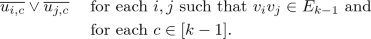  (4)

  Let $D = \overline{u_{i,c}} \vee \overline{u_{j,c}}$ and $\beta = \overline{D}$. From the previous set of $\mathrm {RUP}{}$ inferences in (3) we have

  

  Due to the edge $u_j v_i$ we also have and consequently . Since $\overline{u_{j,c}} \in D$, we have by Lemma 1.

  With the addition of this last set of assumptions, we have effectively copied the edges between $v_i$ to between $u_i$. Figure 3a visualizes the result of this step on $M_4$ with the red edges corresponding to the newly introduced assumptions.

• 5. After the addition of the new edges, we delete the clauses introduced in steps 2, 3, and the clauses corresponding to the edges between U and V of the current Mycielski graph. Figure 3b displays the graph after the deletions.

• 6. Then we inductively repeat steps 2–5, that is, we introduce clauses and delete the intermediate ones for each subgraph isomorphic to Mycielski graphs of descending order. Figure 3c shows the result of repeating the process on a subgraph isomorphic to $M_3$, with the blue edges corresponding to the latest assumptions.

• 7. After an edge is inserted between the two $u_i$ of the subgraph isomorphic to $M_3$, we obtain a k-clique on the two $u_i$ and all of the previous w’s. Then we delete all the clauses corresponding to the edges leaving the clique. This detaches the clique from the rest of the graph as illustrated for $M_4$ in Figure 3d. Since $(k-1)$-colorability of the k-clique is exactly the pigeonhole principle, we simply concatenate a $\mathrm {PR}^-$ proof of the pigeonhole principle as described by Heule et al.  [14], which has maximum discrepancy 2. This completes the $\mathrm {DPR}^-$ proof that $M_k$ is not colorable with $k-1$ colors.

In total, the proof has length $O(3^k k^2)$ and the $\mathrm {PR}$ inferences have maximum discrepancy 2. Hence, by Theorem 2, there also exists a $\mathrm {DSPR}^-$ proof of length $O(3^k k^2)$. Since $\mathrm {MYC}_k$ has length $\Theta (3^k k)$, if we denote the length of the formula by S then the proof is of quasilinear length $O(S \log S)$.    $\square$

Fig. 2.

Schematic form of the argument for the $\mathrm {PR}$ inference. With and , the above diagram shows the transformation we can apply to a solution to obtain another valid solution. A vertex colored black on the inside means that it does not have the outer color, i.e. w has some color other than red. Unit propagation implies that $v_j$ is not colored red.

Fig. 3.

Illustrations of the proof steps in the case where $M_4$ is the initial graph, i.e. $\mathrm {MYC}_4$ is the formula being refuted. The blue and the red edges correspond to the clauses introduced as RUP inferences, and the clauses corresponding to the faded edges are deleted.

Theorem 5

$\mathrm {MYC}_k$ has sublinear-length $\mathrm {PR}^-$ refutations.

Proof

At a high level, the proof is similar to the $\mathrm {DPR}^-$ proof. However, in order to avoid deletion we introduce assumptions at each inductive step that imply the equivalence of every $u_i$ with its corresponding $v_i$. This eliminates the need to detach $M_k'[U]$ from $M_k'[V]$, but leads to sets of vertices forced to have the same color. As a result, the witnesses for the $\mathrm {PR}$ inferences after the first inductive step that refer to switching the color of a vertex $\nu$ need to also include all the previous vertices forced to have the same color as $\nu$.

• 1. We start by introducing the blocked clauses from (1).

• 2. Then we introduce the $\mathrm {PR}$ inferences from (2).

• 3. It becomes possible to infer the following $|U|(k-1)(k-2)$ clauses via $\mathrm {PR}$.

  

  (5)

  Let $\gamma = u_{i,c} \wedge v_{i,c'}$, and denote the conjunction of the formula and the clauses in (1) and (2) by F. In step 3 of the previous proof we showed that . Then, by Lemma 1, we have . Hence, we can switch the color of $v_i$ from $c'$ to c. This does not result in any conflicts since $u_i$ having color c implies that no $v_j \in N(v_i)\cap V$ has the color c, and $\overline{u_{j,c}}$ is implied by unit propagation. As a result, the clause $\overline{u_{i,c}} \vee \overline{v_{i,c'}}$ is $\mathrm {PR}$ with witness $\omega = u_{i,c} \wedge \overline{v_{i,c'}} \wedge v_{i,c}$. After the addition of these clauses, the equivalence $u_{i,c} \leftrightarrow v_{i,c}$ is implied via unit propagation. Due to the edge $v_i v_j$, the existence of the edge $u_i u_j$ is also implied via unit propagation. This step allows us to avoid deletion.

• 4. At this point, we inductively repeat steps 2–3 for each subgraph isomorphic to Mycielski graphs of descending order. However, due to the equivalences $u_{i,c} \leftrightarrow v_{i,c}$, any subsequent $\mathrm {PR}$ inference that argues by way of switching a vertex $\nu$’s color should include in its witness the same color switch for all the vertices that are transitively equivalent to $\nu$ from the previous steps. For instance, if a witness contains $\overline{\nu _{c'}} \wedge \nu _c$, then for each vertex $\eta$ that is equivalent to $\nu$ it also has to contain $\overline{\eta _{c'}} \wedge \eta _c$. The maximum number of such vertices for any $\nu$ occurring in the proof is $\Omega (2^k)$.

• 5. After the $\mathrm {PR}$ clauses are introduced for the subgraph isomorphic to $M_3$, the existence of a k-clique is implied via unit propagation. Figure 4 shows the equivalent vertices and the implied edges after the last inductive step when starting from $M_4$. At the end, we simply concatenate a proof of the pigeonhole principle as before, taking care to include in the witnesses all the equivalent vertices (as described in the previous step) to each vertex whose color is switched by a witness.

The proof has length $O(2^k k^2)$, and $\mathrm {MYC}_k$ has length $\Theta (3^k k)$. Letting S denote the length of the formula, the proof has sublinear length $O(S^{\log _3 2} (\log S)^2)$.    $\square$

Fig. 4.

Equivalent vertices and implied edges. Groups of equivalent vertices are highlighted. Dashed edges are implied by unit propagation.

In the $\mathrm {PR}^-$ proof, the maximum discrepancy is $\Omega (2^k)$. Letting N be the length of the proof, this becomes $\Omega (N/(\log N)^2)$. As a result, we cannot rely on Theorem 2, and the existence of a polynomial-length $\mathrm {SPR}^-$ proof for Mycielski graph formulas remains open. While the existence of such a proof is plausible, we conjecture that it will not be of constant width as the ones we present.

5 Experimental results

All of the formulas, proofs, and the code for our experiments are available at https://github.com/emreyolcu/mycielski.

5.1 Proof verification

In order to verify the proofs we described in the previous section, we implemented two proof generators for $\mathrm {MYC}_k$ and checked the $\mathrm {DPR}^-$ and $\mathrm {PR}^-$ proofs with dpr-trim for values of k from 5 to 10. Figure 5 shows a plot of the lengths of the formulas and the proofs, and Table 1 shows their exact sizes.

Fig. 5.

Plot of the length of the formula and the lengths of the proofs versus k.

Table 1. Formula and proof sizes. For each formula $\mathrm {MYC}_k$, this table shows the number of variables and clauses in the formula, and the lengths of the proofs.

5.2 Effect of redundant clauses on CDCL performance

Suppose we have a proof search algorithm for $\mathrm {DPR}^-$ and that the redundant clauses we introduce in the $\mathrm {DPR}^-$ proof are discovered automatically. Assuming they are found by some method, we look at their effect on the efficiency of CDCL at finding the rest of the proof automatically. In addition, we generate satisfiable instances of the coloring problem (denoted $\mathrm {MYC}_k^+$ and stating that $M_k$ is colorable with k colors) and compare how many of the satisfying assignments remain after the clauses are introduced. The reduction in the number of solutions suggests that the added clauses do a significant amount of work in breaking symmetries.

Let us denote by

• BC: the blocked clauses that we add in step 1,

• PR: the $\mathrm {PR}{}$ clauses that we add inductively in step 2,

• R1: the $\mathrm {RUP}{}$ inferences that we add inductively in step 3,

• R2: the $\mathrm {RUP}{}$ inferences that we add inductively in step 4.

We consider extended versions of the formulas where we gradually include more of the redundant clauses. We cumulatively introduce the redundant clauses from each step, i.e. when we add the PR clauses we also add the BC clauses.

For the satisfiable formulas $\mathrm {MYC}_k^+$, the remaining number of solutions are in Table 2. We used allsat³ to count the exact number of solutions. Adding only the BC or PR clauses drastically reduces the number of solutions. Adding them both leaves a fraction of the solutions.

For the unsatisfiable formulas, we ran CaDiCaL⁴  [3] with a timeout of 2000 seconds on the original formulas and the versions including the clauses introduced at each step. The results are in Table 3. These runtimes are somewhat unexpected as R1 and R2 can be derived from $\mathrm {MYC}{}_k{+}$PR with relatively few resolution steps. One would therefore expect the performance on $\mathrm {MYC}{}_k{+}$PR, $\mathrm {MYC}{}_k{+}$R1, and $\mathrm {MYC}{}_k{+}$R2 to be similar. We study this observation in the next subsection.

Table 2. Number of solutions left in $\mathrm {MYC}_k^+$ after introducing redundant clauses. PR$\setminus$BC is the version of the formula where we add the PR clauses but not the BC ones. For $k\ge 5$, it takes longer than 24 hours to count all solutions, so we only included the results for two small formulas here.

Table 3. CDCL performance on formulas with additional clauses. Each cell shows the time (in seconds) it takes for CaDiCaL to prove unsatisfiability. The cells with dashes indicate that the solver ran out of time before finding a proof.

5.3 Difficult extended Mycielski graph formulas

The CDCL paradigm has been highly successful, because it has been able to find short refutations for problems arising from various applications. However, the above results show that there exist formulas for which CDCL cannot find the short refutations. In particular, the $\mathrm {MYC}{}_k{+}$PR formulas have length $\Theta (3^k k)$ and there exist resolution refutations of length $O(3^k k^3)$: Each clause in R1 and R2, of which there are $O(3^k k^2)$, can be derived in O(k) steps of resolution. As for the clique, it is known that $\mathrm {PHP}_{k-1}$ has resolution refutations of length $O(2^k k^3)$  [4].

This shows that, even if we devise an algorithm to discover the redundant $\mathrm {PR}{}$ clauses automatically, the Mycielski graph formulas still remain difficult for the standard tools. After the clauses in BC and PR become part of the formula, the difficulty lies in deriving the R2 clauses automatically. If we resort to incremental SAT solving  [10] and provide the cubes $u_{i,c} \wedge u_{j,c}$ (negation of each clause in R2) as assumptions to the solver, the formulas become relatively easily solvable. For instance, $\mathrm {MYC}{}_{10}{+}$PR takes approximately 3 minutes on a single CPU. Although it is unlikely that a solver can run this efficiently without any explicit guidance, the small runtime provides evidence that the shortest resolution proof of $\mathrm {MYC}{}_{10}{+}$PR is of modest length.

In this section, we describe a method for discovering useful cubes automatically and using them to solve the $\mathrm {MYC}{}_k{+}$PR formulas. While inefficient, with this method it at least becomes possible to find proofs of these formulas in a matter of minutes, compared to CDCL which did not succeed even with a timeout of three days on $\mathrm {MYC}_{10}{+}$PR. Given a formula F, the below procedure discovers binary clauses, inserts them to F, and attempts to solve F via CDCL.

• 1. Iteratively remove the clause that has the largest number of resolution candidates until the formula becomes satisfiable. For $\mathrm {MYC}{}_k{+}$PR, this corresponds to simply removing the clause $w_1 \vee \ldots \vee w_{k-1}$. Call the newly obtained formula, which is satisfiable, $F^-$.

• 2. Repeat:

  • (a) Sample M satisfying assignments for $F^-$ using a local search solver (we used YalSAT⁵  [2]).

  • (b) Find all pairs of literals $(l_i, l_j)$ that do not appear together in any of the solutions sampled so far. Form a list with the cubes $l_i \wedge l_j$, and shuffle it in order to avoid ordering the pairs with respect to variable indices. In the case of $\mathrm {MYC}{}_k{+}$PR, the clause $\overline{u_{i,c}} \vee \overline{u_{j,c}}$ is implied by $F^-$, hence $(u_{i,c}, u_{j,c})$ must be among the pairs found.

  • (c) If the number of pairs found did not decrease by more than 1 percent after the latest addition of satisfying assignments, break.

• 3. Repeat:

  • (a) Partition the remaining cubes into P pieces. Use P workers in parallel to perform incremental solving with a limit of L conflicts allowed on the instances of the formula F using each separate piece as the set of assumptions. Aggregate a list of refuted cubes.

  • (b) For each refuted cube B, append $\overline{B}$ to the formula F.

  • (c) If the number of refuted cubes is less than half of the previous iteration, break.

• 4. Run CDCL on the final formula F that includes negations of all the refuted cubes.

Table 4 displays the results for formulas with $k\in \{7,\ldots ,10\}$ and varying numbers of parallel workers P.

Table 4. Results on finding proofs for $\mathrm {MYC}_k{+}$PR. From left to right, the columns correspond to the number of samples used for obtaining a list of cubes, the number of cubes obtained after filtering pairs of literals, time it takes to sample solutions using a local search solver with 20 workers and filter pairs of literals, maximum number L of conflicts allowed to the incremental SAT solver, number of parallel workers P, total time it takes to refute cubes and prove unsatisfiability of the final formula F, percentage of time spent in the final CDCL run on F, number of iterations spent refuting cubes and adding them to the formula.

6 Conclusion

We showed that there exist short $\mathrm {DPR}^-$, $\mathrm {DSPR}^-$, and $\mathrm {PR}^-$ proofs of the colorability of Mycielski graphs. Interesting questions about the proof complexity of $\mathrm {PR}$ variants remain. For instance, $\mathrm {DPR}^-$ has not been shown to separate from $\mathrm {ER}$ or Frege, and even simpler questions regarding upper bounds for some difficult tautologies are open. It is also unknown, although plausible, whether there exists a polynomial-length $\mathrm {SPR}^-$ proof of the Mycielski graph formulas.

Apart from our theoretical results, we encountered formulas with short resolution proofs for which CDCL requires substantial runtime. We developed an automated reasoning method to solve these formulas. In future work, we plan to study whether this method is also effective on other problems that are challenging for CDCL.

References

The On-Line Encyclopedia of Integer Sequences. Published electronically at https://oeis.org/A122695
Biere, A.: CaDiCaL, Lingeling, Plingeling, Treengeling, YalSAT entering the SAT competition 2017. In: Proceedings of SAT Competition 2017 – Solver and Benchmark Descriptions. vol. B-2017-1, pp. 14–15 (2017)
Biere, A.: CaDiCaL at the SAT Race 2019. In: Proceedings of SAT Race 2019 – Solver and Benchmark Descriptions. vol. B-2019-1, pp. 8–9 (2019)
Buss, S., Pitassi, T.: Resolution and the weak pigeonhole principle. In: Computer Science Logic, pp. 149–156 (1998)
Buss, S., Thapen, N.: DRAT proofs, propagation redundancy, and extended resolution. In: Theory and Applications of Satisfiability Testing – SAT 2019. pp. 71–89 (2019)
Caramia, M., Dell’Olmo, P.: Coloring graphs by iterated local search traversing feasible and infeasible solutions. Discrete Applied Mathematics 156(2), 201–217 (2008)
Cook, S.A., Reckhow, R.A.: The relative efficiency of propositional proof systems. The Journal of Symbolic Logic 44(1), 36–50 (1979)
Crawford, J.M., Ginsberg, M.L., Luks, E.M., Roy, A.: Symmetry-breaking predicates for search problems. In: Proceedings of the Fifth International Conference on Principles of Knowledge Representation and Reasoning. pp. 148–159 (1996)
Desrosiers, C., Galinier, P., Hertz, A.: Efficient algorithms for finding critical subgraphs. Discrete Applied Mathematics 156(2), 244–266 (2008)
Eén, N., Sörensson, N.: Temporal induction by incremental SAT solving. Electronic Notes in Theoretical Computer Science 89(4), 543–560 (2003)
Goldberg, E., Novikov, Y.: Verification of proofs of unsatisfiability for CNF formulas. In: Proceedings of the Conference on Design, Automation and Test in Europe (DATE 2003). pp. 886–891 (2003)
Heule, M.J.H., Biere, A.: What a difference a variable makes. In: Tools and Algorithms for the Construction and Analysis of Systems. pp. 75–92 (2018)
Heule, M.J.H., Kiesl, B., Biere, A.: Clausal proofs of mutilated chessboards. In: NASA Formal Methods. pp. 204–210 (2019)
Heule, M.J.H., Kiesl, B., Biere, A.: Strong extension-free proof systems. Journal of Automated Reasoning 64(3), 533–554 (2020)
Kullmann, O.: On a generalization of extended resolution. Discrete Applied Mathematics 96–97, 149–176 (1999)
Marques-Silva, J.P., Sakallah, K.A.: GRASP—a new search algorithm for satisfiability. In: Proceedings of the 1996 IEEE/ACM International Conference on Computer-Aided Design. pp. 220–227 (1997)
Mycielski, J.: Sur le coloriage des graphs. Colloquium Mathematicae 3(2), 161–162 (1955)
Ramani, A., Aloul, F.A., Markov, I.L., Sakallah, K.A.: Breaking instance-independent symmetries in exact graph coloring. In: Proceedings of the Conference on Design, Automation and Test in Europe (DATE 2004). pp. 324–329 (2004)
Schaafsma, B., Heule, M.J.H., van Maaren, H.: Dynamic symmetry breaking by simulating Zykov contraction. In: Theory and Applications of Satisfiability Testing – SAT 2009. pp. 223–236 (2009)
Trick, M.A., Yildiz, H.: A large neighborhood search heuristic for graph coloring. In: Integration of AI and OR Techniques in Constraint Programming for Combinatorial Optimization Problems. pp. 346–360 (2007)
Van Gelder, A.: Another look at graph coloring via propositional satisfiability. Discrete Applied Mathematics 156(2), 230–243 (2008)
Vinyals, M.: Hard examples for common variable decision heuristics. In: Proceedings of the Thirty-Fourth AAAI Conference on Artificial Intelligence (2020)
Zhou, Z., Li, C.M., Huang, C., Xu, R.: An exact algorithm with learning for the graph coloring problem. Computers and Operations Research 51, 282–301 (2014)
Zhu, Q., Kitchen, N., Kuehlmann, A., Sangiovanni-Vincentelli, A.: SAT sweeping with local observability don’t-cares. In: Proceedings of the 43rd Annual Design Automation Conference. pp. 229–234 (2006)
Acknowledgements
This work has been supported by the National Science Foundation (NSF) under grant CCF-1813993.
Author information
Authors and Affiliations
Corresponding author
Editor information
Editors and Affiliations
Rights and permissions
Copyright information
© 2020 Springer Nature Switzerland AG
About this paper
Cite this paper
Yolcu, E., Wu, X., Heule, M.J.H. (2020). Mycielski Graphs and PR Proofs. In: Pulina, L., Seidl, M. (eds) Theory and Applications of Satisfiability Testing – SAT 2020. SAT 2020. Lecture Notes in Computer Science(), vol 12178. Springer, Cham. https://doi.org/10.1007/978-3-030-51825-7_15
Download citation
DOI: https://doi.org/10.1007/978-3-030-51825-7_15
Published:
Publisher Name: Springer, Cham
Print ISBN: 978-3-030-51824-0
Online ISBN: 978-3-030-51825-7
eBook Packages: Computer ScienceComputer Science (R0)