
Abstract
The moisture transfer process in multilayered building components with an interface is very different than the moisture transfer considered when having different materials/layers separately. Quantifying moisture transfer in multi-layered systems through numerical simulations is essential to predict the real behaviour of those building materials in contact with moisture, which depends on the climatic conditions. Unfortunately, the contact phenomenon is neglected in numerical simulations which compromise the feasibility of the results. In this work, the moisture transfer in multi-layered building components is analysed in detail, for perfect contact and hydraulic contact interface. The “knee point” was detected, numerically, in water absorption curves and the moisture-dependent interface resistance was quantified and validated for transient conditions. The methodology proposed to detect the “knee point” can be also used in the future for different multilayer materials with an interface, in order to obtain more correct maximum hygric resistance values, to be used in future numerical simulations.
Access provided by Autonomous University of Puebla. Download chapter PDF
Keywords
1 Introduction
Moisture transfer in construction building components is fundamental for the durability of built elements, influencing the thermal behaviour and consequently the energy consumption in the building and occupants’ health by the air quality. There are such demonstrative problems due to moisture like frost/defrost damage in facades, mould on interior surfaces, fungus in floors and walls by rising damp, deterioration in floors and walls by flood occurrences, degradation of walls and roofs by internal condensations, etc.
For example, the study of rising damp phenomenon allowed the investigation of a technique to solve this problem that can already be used, with the necessarily revisions, to treat building walls after a flood (Delgado et al. 2016; Barreira et al. 2016 Guimarães et al. 2012, 2013; Freitas et al. 2011. In Portugal we have historical buildings near water courses with degraded walls by the permanence of water. Moisture in buildings can have different origins and rising damp is probably the most current one. Floods are extreme occurrences but can introduce large amounts of water in the walls. In conclusion, rising damp, because of its high occurrence frequency, and floods, because of the seriousness of their consequences, represent both a high risk in terms of building humidity.
The analysis of moisture migration in building materials and elements is crucial for its behaviour knowledge also affecting its durability, waterproofing, degradation and thermal performance. A building wall, generally, consists of multiple layers, and thus the investigation of the moisture transfer presumes knowledge about the continuity between layers. de Freitas (1992, 1996) considered three different interfaces configurations:
-
1.
Perfect contact—when there is contact without interpenetration of both layers porous structure;
-
2.
Hydraulic continuity—when there is interpenetration of both layers porous structure;
-
3.
Air space interface—when there is an air box of a few millimetres wide between layers.
In resume, the most common interfaces types are perfect contact (ex: blocks in contact), hydraulic contact (mortar between the masonry blocks) and air space. It is necessary to have thorough knowledge regarding the building constituent material (red clay, concrete, granite, etc.).
Derdour et al. (2000) analysed the effect of thickness, porosity and the drying conditions of several building materials on the drying time constant. Bednar (2002) studied the influence of the following properties: material size and insulation, and climate conditions on the liquid moisture transport coefficient during drying experiments. Karoglou et al. (2005) evaluated the effect of environmental conditions, such as air temperature, air relative humidity and air velocity, on the drying performance of 4 stone materials, 2 bricks and 7 plasters. However, the study of multi-layered masonry walls with imperfect contact, as the hydraulic interface, is practically inexistence in literature.
Considering the contact phenomena in multi-layered building components, like brick-mortar composites, or even mortar-brick-isolation-mortar solutions, the moisture transfer process and the obtained values differs from the moisture transfer considered when having different materials/layers separately (de Freitas 1992). In fact, the interface promotes a hydric resistance which means that becomes a slowing of the moisture transport across the material interface. The study of liquid transport across this interface configuration (ceramic brick and mortar) implies the correct knowledge of the hygrothermal mechanical and thermal properties of the build materials employed.
There is still a high unawareness regarding the influence of the interfaces between layers. Some studies which have been carried out conclude that it is important to analyse and consider the interface correctly. In the hydraulic contact like, for example, a mortar joint, it is important to understand that in the curing process water will be transported (Davison 1961; Groot 1995; Holm et al. 1996; Brocken et al. 1998; Hendrickx et al. 2009; Derluyn et al. 2011) which contributes to the modification of mortar properties. More, there is an interpenetration between the solid structural material that is in contact with the mortar which means that occurs changing in the pore structure of the material in contact (Brocken et al. 1998; Derluyn et al. 2011), in a certain thickness. This result in the continuity of the pore structure, i.e., the thermal and hydric flows that go out by layer 1 is the same that go in layer 2. There is continuity in capillary pressure but the water content in the first layer is different from the water content in the second layer.
In numerical simulations, some authors include hydraulic contact phenomena. As example, Brocken (1998) calculates only a change in the mortar properties neglecting the change in contact properties by assuming a perfect hydraulic interface contact. Qiu et al. (2003) and de Freitas et al. (1992) only consider an interface resistance, however, Derluyn et al. (2011) consider both cases, a change in mortar properties and an interface resistance.
Thus, the interface resistance can be calculated experimentally by the mass variation curve as a function of time, in a water absorption test, and correspond to the curve pendant after hit the discontinuity, i.e. the interface. The problem is to correctly detect the pendant which can be made if the “knee point” (transition) can be reached.
In this paper, the moisture transfer in multi-layered building components is analysed. The existence of different types of interfaces (perfect contact and hydraulic contact interface) contributes to different means of moisture transport when compared to a monolithic porous element. As examples, the “knee point” was detected in water absorption curves of multi-layered building components with different interfaces. It was presented a “knee point” measurement procedure, which is automatic and has proved to be accurate. To fully achieve this objective, herein it is proposed the use of an automatically changing point detection method to assist the water absorption analysis. In fact, the manual procedure can be highly time-consuming. In addition to the time saved, there is, as well, still an increase in accuracy, which does not depend on the result of the operator. This methodology to detect the “knee point” can also be used in the future for different materials with interfaces.
Finally, the moisture-dependent interface resistance between brick building components was quantified and validated for transient conditions which mean that can be used for future numerical simulations.
2 Moisture Transfer Across Material Interfaces
Moisture transfer across material interfaces is influenced by a number of phenomena and directly depends on the interface type. In the hydraulic contact like, for example, a mortar joint, it is important to understand that in the curing process water will be transported (Davison 1961; Groot 1995; Holm et al. 1996; Brocken et al. 1998) which contributes to the modification of the mortar properties. Concurrently, there is an interpenetration between the solid structural material that is in contact with the mortar which means that occurs changing in the pore structure of the material in contact with mortar (Hendrickx et al. 2009; Derluyn et al. 2011), in a certain thickness. This results, for hydraulic contact, in a continuity of the pore structure where the thermal flow that goes out in the layer 1 is the same that goes in the layer 2, there is continuity in temperature profiles, the hygric flow that goes out in the layer 1 is the same that goes in in the layer 2 and there is continuity in capillary pressure but the moisture content in the first layer is different from the moisture content in the second layer (W1 ≠ W2). In hydraulic contact phenomena, the equality of the capillary pressure (Pc1 = Pc2) allows the determination of a relation between the moisture content of both materials (W1 = R.W2), in the interface, through a function R(Pc) that can be determined as sketched in Fig. 1.

Function R determination
In the air space interface where two solid layers are separated by an air space with some millimetres it can be considered that, in isothermal regime, the hygric flow that goes out in the layer 1 is the same that goes in in the layer 2 being this value limited by the maximum vapour value transported by the air space that depends on the vapour pressure of both surfaces and on the air thickness. In addition, if the water content of the layer with higher value is lower than the critical water content (Wcr) there is continuity in the relative humidity in the air space interface φ1 = φ2, if the water content of one layer is higher than the Wcr the other layer presents a water contact that goes to the critical value of that material. The equality of the relative humidity φ1 = φ2 means that it can be established a relation between the water content in the interface (W1 = S.W2) considering a function S that can be determined as described in Fig. 2.

Function S determination
In numerical simulations, when more than one consolidates material is separated by air space there is a capillary break that avoids the transport of liquid water being all the transport made in the vapour phase. In the perfect contact, i.e., a contact without interpenetration of both layers’ porous structure, it can be assumed that there is continuity of temperature and equality of thermal flows at the entrance and exit, on the interface. About the humidity, experimental studies showed that the discontinuity of the porous structure generates a hygric resistance that imposes a maximum flow transmitted, FLUMAX, Fhum1 = Fhum2 ≤ FLUMAX. In addition, the capillary pressure is different in both interface materials.
In numerical simulations, it must be considered a hygric resistance that imposes a maximum flow transmitted, FLUMAX, which should be calculated experimentally. In practice, however, commonly neither a change in material properties nor interface resistances are taken into account in the current numerical simulations. Only a limited number of studies have determined an interface resistance (Qiu et al. 2003; Brocken 1998) or analysed the change in mortar properties (Derluyn et al. 2011; Brocken 1998; Vereecken and Roels 2014) while both are probably strongly case-dependent; furthermore, those studies all assume a constant value for the interface resistance. Particularly, in perfect contact and hydraulic contact interface a limited number of studies have determined an interface resistance considering the difficulty and time consuming experimental test that should be made to estimate this parameter.
3 Materials and Methods
The water absorption curve increases over time and then presents instants (points of change) where the rate of absorption seems to decrease significantly. These instants correspond to the contact of the water with a different material (contact with the interface). Only one point of change is expected for the interfaces in perfect contact and air space interface (see Fig. 3a), different from what happens with for the hydraulic interfaces (see Fig. 3b) where we can observe two discrete knees, one before the interface and another when the interface is saturated.

Water absorption curve and the changing instant, knee point
This study can be applied to other cases of interfaces. This generalization will be presented later. Since the goal is to address the effect of the interface in water absorption, the water resistance is measured immediately after the first changing point, which is the time interval of interest. The final measurement is performed by calculating each Hygric Resistance (RH). Figure 4 depicts how the several values are measured.

Method for hygric resistance measurements
Considering this measuring procedure, it is important to detect the exact time instant of the “knee point” automatically and with some precision. In the literature, there are several methods of knee or jump point detection (Ville Satopaa et al. 2011; Wang and Tseng 2013; Zhao et al. 2008a, b; Christopoulos 2014; Du et al. 2014). The following three methods were taken into consideration to develop the algorithm presented in this work. The choice of these methods took into account the fact that there are discrete methods, intuitive and easy to implement, available in the literature. The following two methods were considered to develop the algorithm presented in this work:
-
1st Method: This method considers a line which passes through the two extreme points observed (x0 and xn). It also considers a set of line segments perpendicular to this line, where each line segment begins at an observed point (xi = (ti, Mwi)) and ends at a point of the line. The knee point is defined as the point related to the greater segment (Ville Satopaa et al. 2011), as described in Fig. 5 and Annex 1—SEC.Program (an algorithm developed by the authors).
Fig. 5 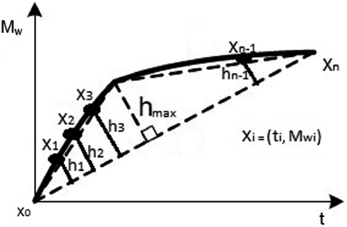
Knee point determination by the 1st method
-
2nd Method: In this method, the point where the pair of lines that best approaches the curve is called “knee”. For its determination, it is necessary to perform, for each point (xi = (ti, Mwi) of the curve, two linear fittings, one for all points to the left of xi and one for all points to the right of xi. The knee is considered the point that minimizes the sum of the errors for the two fittings. This method is implemented in Matlab in a function called “knee-pt.m”.
-
3rd Method: This method is a combination of the two methods previously presented. Since the main goal of the algorithm proposed is to find the “knee” point of a set of points xi = (ti, Mwi), i = 1, 2, …, n obtained in the measuring procedure, where the data errors should be taken into account, the combination of the two previously presented methods can give a better knee point.
-
The steps of this algorithm are (see Annex 2—Hybrid.program, an algorithm developed by the authors):
-
1.
Use the 1st Method to calculate, for each point obtained in the measuring procedure, the length of the line segment that is perpendicular to the line that connects the two extreme points of the set. Sort the length of perpendicular line segment by a decreasing order. Let \( M1 \) be the set of indices of the points corresponding to this ordering.
-
2.
Use the 2nd Method to determine the sum of the errors for the two linear fittings found for each point obtained in the measuring procedure. Sort the sum of the errors for the two linear fittings by an ascending order. Designate by \( M2 \) the set of indices of the points associated with this ordering.
-
3.
Determination of the knee point. Find the point xi = (ti, Mwi) whose index, i, occupies the best positions in sets M1 and M2, using the following algorithm:
-
Step 0—Let \( k = 1 \) be the position of an element in a set, \( i = 1 \) an index position and \( n \) the total number of points obtained in the measuring procedure.
-
Step 1—If \( i > k \), let \( j = 1 \) and go to Step 3.
-
Step 2—If \( M1\left( k \right) = M2\left( i \right) \), the knee point is \( \left( {t\left( {M1\left( k \right)} \right), Mwi\left( {M1\left( k \right)} \right)} \right) \) and Stop the algorithm. Otherwise, let \( i = i + 1 \) and return Step 1.
-
Step 3—If \( j \ge k \), go to Step 5.
-
Step 4—If \( M2\left( k \right) = M1\left( j \right) \), the knee point is \( \left( {t\left( {M2\left( k \right)} \right), Mwi\left( {M2\left( k \right)} \right)} \right) \) and Stop the algorithm. Otherwise, let \( j = j + 1 \) and return Step 3.
-
Step 5—Let \( k = k + 1 \). If \( k > n, \) an error message must be sent. Otherwise, let \( i = 1 \) and return Step 1.
-
-
1.

4 Experimental Setup
The experimental procedure has been described to guarantee consistent measurements of hygric resistance in multilayer building materials and to “knee point” detection in water absorption curves. The hygric resistance was determined after the knee point of several curves, and for each curve, it was computed several dispersion measures to evaluate the consistency. The measures were the coefficient of variation.
In this work, two different ceramic blocks of red brick were tested with a sample similar size: ceramic A with 4 × 4 × 10 cm and ceramic B with 5 × 5 × 10 cm (see Fig. 6). Several standards can be applied for the experimental determination of bulk density, as ISO 10545-3 (1995) for ceramic tiles, EN 12390-7 (2009) for concrete, EN 772-13 (2000) for masonry units. The samples must be dried until a constant mass is reached. The samples volume was calculated based on the average of three measurements of each dimension.

Specimen’s designation and configuration—water absorption tests
Porosity or void fraction is a measure of the void spaces in a material, and is a fraction of the volume of voids over the total volume, between 0 and 1 (see Fig. 7). The standard ISO 10545-3 (1995) for ceramic tiles was used to measure the bulk porosity. The building materials porous characteristics have an important influence on the mechanisms of moisture transfer. The porous network, formed by cavities and channels, is the medium through which a fluid (liquid or vapour) are propagated. This type of porosity, called open porosity, is characteristic of most building materials. In this study, it was used an automated mercury porosimeter (Poremaster-60 Quantachrome) and a helium pycnometer The mercury porosimeter allowed to determine the pore size distribution up to 0.0035 micrometres in diameter, as well as the total surface area normalized to the sample mass and bulk density.

Material porous structure
It is important to be noted that there is a relation between the mortars and the sample properties in the masonry performance related to water penetration resistance. The mortar properties considered in the study include compressive strength, workability, water retention, and porosity. The properties of masonry elements include surface texture; porosity and the initial rate of absorption (Ghosh and Melander 1991).
Since the building walls present mortars with average values of porosity and a large number of pores that allow the capillary action and movement of water inside the coating system, the presence of moisture can be observed, mainly in the lower part of the walls. Mortars are characterized by the presence of voids within the materials (pores), which may vary according to the water/cement ratio, as well as the granulometry of the aggregates used in the mortar.
The moisture transport is strongly dependent on the complex morpho-optic aspect of the porous space. The pores, free spaces distributed inside the solid structure, characterize the permeability of the medium, allowing the fluid flow (Mendes and Philippi 2005).
The experiments to determine the interface influence, conducted in this study, are guided by the outline of the partial immersion method as explained by the standard ISO 15148 (2002). Specimens of two different red bricks, A and B, were tested (see Fig. 8). During the tests, the temperature and the relative humidity was also measured (see Fig. 8).

Imbibition model used in the research
All the specimens were sealed in the lateral faces with an epoxy coating to avoid the evaporation through these sides and assure the unidirectional moisture flow from the bottom to the specimens’ top surface.
Capillary absorption data were obtained by placing samples in distilled water. Their base was submerged only a few millimetres (~1–5 mm) in order to avoid build-up of hydrostatic pressure. The environmental laboratory conditions were approximately 23 °C of temperature and 50% of relative humidity (φ), during the experiments duration. Experiments were conducted for immersion periods from several minutes to about 20 days. The samples were placed in a constant-temperature water bath controlled within ±0.5 °C to avoid changes in liquid viscosity that might affect the absorption rate (Mukhopadhyaya et al. 2002; Delgado et al. 2006; Guimarães et al. 2018). After soaking, the moisture content of samples was calculated based on the increase in the sample weight at corresponding times. For this purpose, at regular time intervals, ranging from 5 min at the beginning to 12 h during the last stages of the process, the samples were rapidly removed from the water bath and superficially dried on a large filter paper to eliminate the surface liquid. The samples were then weighed to determine the moisture uptake. The samples were subsequently returned into the analysed solution via wire mesh baskets and the process was repeated, consequently.
5 Results and Discussion
In this study, two different ceramic blocks of red brick were tested with similar size samples: ceramic A with 4 × 4 × 10 cm3 and ceramic B with 5 × 5 × 10 cm3. The density and porosity of the tested materials were measured carefully and the obtained values are summarized, in Table 1. Also, Table 1 presents the absorption coefficients obtained, i.e., 0.10 kg/m2s0.5 and 0.19 kg/m2s0.5, for the monolithic samples of red brick type “A” and “B”, respectively (see Fig. 8). The absorption coefficient of red brick type “B” is approximately two times higher, an expectable result as the density of this material is greater than the density of red brick type “A”. The water vapour diffusion resistance factor, μ, is given by \( \mu = {{\delta_{p} } \mathord{\left/ {\vphantom {{\delta_{p} } {\delta_{a} }}} \right. \kern-0pt} {\delta_{a} }} \), where δa is the vapour permeability of the air. The results obtained showed that the average values of the water vapour diffusion resistance factor for ceramic block A samples were in the order of 33.1 (corresponding to 5.94 × 10⁻¹² kg/msPa) for drycup, while for ceramic block “B” samples it was 21.4 (corresponding to 9.07 × 10⁻¹² kg/msPa) for the drycup. For these values, it is possible to conclude that the ceramic block “B” samples always presented lower values of water vapour diffusion resistance factor when compared to the ceramic block “A” samples.
Table 1, also, described the experimental results obtained for the physical and hygrothermal characterization of cement mortar and lime mortar samples analysed. The results showed that the two mortars tested present similar values of bulk density and porosity, however, cement mortar presents highest values of moisture content, w80% and wsat and lower values of water vapour permeability.
The average mass variation per contact area in the capillary absorption process for the mortar samples tested. The experimental assessment of the water absorption coefficients showed a slight difference of values between the two mortars tested. The averages values obtained are 0.153 ± 0.012 kg/m2 s0.5 and 0.124 ± 0.002 kg/m2 s0.5, for cement mortar and lime mortar, respectively. The coefficient of variation found for each set of identical samples was approximately 7.8% for cement mortar and 1.4% for lime mortar.
A schematic plot of the increase in weight of the test specimen versus the time indicates that the specimen weight increases before it comes close to the saturation limit (see Figs. 9 and 10). These Figures show that the samples with perfect contact and hydraulic contact interface present similar behaviour, before the interface, with the monolithic samples, however, when water reaches the interface a water resistance is verified, reducing the absorption rate. As expected, the results showed a decrease of the absorption rate for samples with hydraulic contact (cement mortar and lime mortar) and perfect contact, in comparison with the monolithic samples. Also, it is possible to observe a decrease of the absorption rate for samples with cement mortar interface comparatively to the lime mortar materials (Guimarães et al. 2018). As described by Nunes et al. (2017) the changing of porosity in mortar near the transition zone of brick-mortar can be attributed to the flow of water from fresh brick during the bonding process. In the beginning, small binder particles can be transported to the mortar-brick interface and the plaster becomes more compact (enriched in binder) in the interface.

Water absorption curves of the monolithic sample and samples with perfect contact: a for red brick type “A” and b red brick type “B”

Water absorption curves of the monolithic sample and samples with hydraulic contact (cement and lime mortar): a for red brick type “A” and b red brick type “B”
Another conclusion observed was as further away from the base is located the interface, higher is the water absorbed. The interface could significantly retard the flow of moisture transport. i.e., the discontinuity of moisture content across the interface indicated that there was a difference in capillary pressure across the interface.
For the gravimetric method analyse the “knee point” is determined manually and the hygric resistance (RH) is calculated experimentally (during a water absorption test) by the slope of the mass variation curve as function of time, after the knee point:
where Δt and ΔMw are the variation of the time and water absorption immediately after the knee point, respectively. Considering this measuring procedure, it is important to detect this instant with precision and automatically. To fulfil this propose, it is intended to use a changing point automatic detection method to assist the water absorption analysis.
The three methods presented above were applied to the experimental data reported with the interface at three different heights (at 2 cm of the base, at 5 cm and at 7 cm) of perfect contact and hydraulic contact interface and two types of bricks. The results for the determination of the “knee point” of 20 cases showed:
-
In 3 cases, the three methods obtained the same knee point;
-
In 10 cases, each method obtained a distinct point as a knee;
-
In 1 cases, the 2nd and 3rd methods obtained the same point as the knee, but the 1st method produced another distinct point;
-
In 6 cases, the 1st and 3rd methods obtained the same point as knee but the 2nd method produced another distinct point;
-
No cases were observed in which the 1st and 2nd methods obtained the same knee point and the 3rd method produced another distinct point.
Figure 11 shows some particular cases. In this figure, black asterisks represent all points obtained in the measuring procedure, magenta circle denotes the knee attained by the 1st method, red square symbolizes the knee determined by the 2nd Method and blue diamond characterizes the knee reached by the 3rd method.

a The three methods obtained the same knee point; b each method obtain a distinct point as a knee; c only the 2nd and 3rd methods obtained the same point as the knee; and d Only the 1st and 3rd methods obtained the same point as the knee (magenta circle—knee attained by the 1st method, red square—knee determined by the 2nd method and blue diamond—knee reached by the 3rd method)
It should be noted that when the three methods do not obtain the same knee, the point determined by the 2nd method is always to the left of the point calculated by the 3rd method. Meanwhile, the point obtained by the 1st method is always to the right of the point attained by the 3rd method.
The 3rd method is an optimization of the existent ones, 1st and 2nd, and showed to be the best method in the experimental cases analysed, with a good detection of the knee point. It is important to keep in mind that in this type of analyse is, usually, used with experimental data, which means that there are “discrete” points, and not a curve, with some possible outliers that sometimes contribute to wrong solutions using other methodologies. Finally, the gravimetric method includes 12 with an error ratio lesser than 20% in relation to the new methodology. When speaking of an error ratio in the order of 30%, the cases increase to 14 for gravimetric method (GM) compared to new method (NM).
The results presented in Table 2 shows good accordance similarity between the hygricv resistance values obtained by gravimetric method and the new methodology proposed. It is possible to observe that for higher positions of the interface the water absorbed is higher and the hygric resistance is lower. It was expected that considering an interface between layers the water absorption would become lower, and for the case of interfaces located in higher positions the absorption would become higher as the discontinuity is reached latter.
It is important to be in mind that if we place the interface at different distances from the wetting plane the beginning of the slowing of the wetting occurs in different time periods, as expected, however, from that moment onwards, there is an increase in mass that, in the limit, is constant for all cases.
6 Conclusions
In conclusion, the main achievements related to the new methodology proposed for “knee point” detection are the following:
-
There is still a high unawareness regarding the influence of the building components interfaces between layers in moisture transfer processes;
-
The existence of different types of interface (perfect contact, hydraulic contact, and air space interface) contributes to different ways of moisture transport when compared to a monolithic porous element;
-
The “knee point” was detected in water absorption curves which mean the hygric resistance was measure in perfect contact multilayer building components. Moreover, when the contact between the different materials is hydraulic, i.e., there are two points of change, the user can define the time-space in which the knee is to be determined and run the program more than once if you want to determine the two knees;
-
The moisture-dependent interface resistance between brick building components was quantified and validated for transient conditions which can be used for future numerical simulations;
-
Two methodologies were studied to detect the knee point;
-
A 3rd methodology is proposed, optimizing the other two, which showed to be the best method for cases presented;
-
The proposed methodology is especially important considering that it is usually used in conjunction with experimental data which means that there are “discrete” points, and not a curve, with some possible outliers that sometimes contribute to wrong solutions using other methodologies;
-
The proposed methodology to detect the “knee point” can be also used in the future for different materials;
-
From the computational experimental performed, it is shown that the method developed in this work (3rd method) determines a point that best fits the definition of the knee;
-
In order to make this process even more efficient and effective, the program allows the user to choose whether to define the time frame in which to determine the knee;
-
Finally, in case there is an air space between the different materials, the procedure is the same that was presented for the perfect contact.
References
Barreira E, Almeida R, Delgado JMPQ (2016) Infrared thermography for assessing moisture related phenomena in building components. Constr Build Mater 110:251–269. https://doi.org/10.1016/j.conbuildmat.2016.02.026
Bednar T (2002) Approximation of liquid moisture transport coefficient of porous building materials by suction and drying experiments. demands on determination of drying curve. In: Proceedings of the 6th Symposium on Building Physics, Nordic Countries, Trondheim, Norway, pp 493–500
Brocken HJP (1998) Moisture transfer in brick masonry: the grey area between bricks, T.U. Eindhoven, The Netherlands, Ph.D. thesis
Brocken HJP, Spiekman ME, Pel L, Kopinga K, Larbi JA (1998) Water extraction out of mortar during brick laying: a NMR study. Mater Struct 31(1):49–57
Christopoulos DT (2014) Reliable computations of knee point for a curve and introduction of a unit invariant estimation. https://doi.org/10.13140/2.1.3111.5844
Davison JI (1961) Loss of moisture from fresh mortars to bricks. Mater Res Stand ASTM 1:385–388
de Freitas VP (1992) Moisture transfer in building walls—Interface phenomenon analysis, Faculdade de Engenharia da Universidade do Porto, Porto, Portugal, Ph.D. thesis [in Portuguese]
de Freitas VP, Abrantes V, Crausse P (1996) Moisture migration in building walls: analysis of the interface phenomena. Build Environ 31:99–108. https://doi.org/10.1016/0360-1323(95)00027-5
Delgado JMPQ, Ramos NMM, Freitas VP (2006) Can moisture buffer performance be estimated from the sorption kinetics? J Build Phys 29(4):281–299. https://doi.org/10.1177/1744259106062568
Delgado JMPQ, Guimarães AS, de Freitas VP, Antepara I, Kočí V, Černý R (2016) Salt damage and rising damp treatment in building structures. Adv Mater Sci Eng 2016:13, Article number ID 1280894. https://doi.org/10.1155/2016/1280894
Derdour L, Desmorieux H, Andrieu J (2000) A contribution to the characteristic drying curve concept: application to the drying of plaster. Dry Technol 18(1–2):237–260
Derluyn H, Janssen H, Carmeliet J (2011) Influence of the nature of interfaces on the capillary transport in layered materials. Constr Build Mater 25(9):3685–3693
Du W, Leung SYS, Kwong CK (2014) Time series forecasting by neural networks: a knee point-based multi-objective evolutionary algorithm approach. Expert Syst Appl 41(18):8049–8061. https://doi.org/10.1016/j.eswa.2014.06.041
EN ISO 10545-3 (1995) Ceramic tiles—Part 3: determination of water absorption, apparent porosity, apparent relative density and bulk density. Geneva, Switzerland
EN ISO 12390-7 (2009) Testing hardened concrete. Density of hardened concrete. Geneva, Switzerland
EN ISO 772-13 (2000) Methods of test for masonry units. Determination of net and gross dry density of masonry units (except for natural stone)
Freitas VP, Guimarães AS, Delgado JMPQ (2011) The HUMIVENT device for rising damp treatment. Recent Patents Eng 5:233–240. https://doi.org/10.2174/187221211797636863
Ghosh SK, Melander JM (1991) Air content of mortar and water penetration of masonry walls. Masonry Information, Portland Cement Association
Groot CJWP (1995) Effects of water on mortar-brick bond. Heron J 40:57–70
Guimarães AS, Delgado JMPQ, Freitas VP (2012) Rising damp in building walls: the wall base ventilation system. Heat Mass Transf 48:2079–2085. https://doi.org/10.1007/s00231-012-1053-3
Guimarães AS, Delgado JMPQ, Freitas VP (2013) Rising damp in walls: evaluation of the level achieved by the damp front. J Build Phy 37:6–27. https://doi.org/10.1177/1744259112453822
Guimarães AS, Delgado JMPQ, Azevedo AC, Freitas VP (2018) Interface influence on moisture transport in buildings. Constr Build Mater 162:480–488. https://doi.org/10.1016/j.conbuildmat.2017.12.040
Hendrickx R, Van Balen K, Van Gemert D, Roels S (2009) Measuring and modeling water transport from mortar to brick. Building materials and building technology to preserve the built heritage. In: 1st WTA-international Ph.D. symposium, vol 33, pp 175–194
Holm A, Krus M, Künzel HM (1996) Feuchtetransport über Materialgrenzen im Mauerwerk. Rest Build Monum 2(5):375–396
ISO 15148 (2002) Hygrothermal performance of building materials and products–Determination of water absorption coefficient by partial immersion. Genève, Switzerland
Karoglou M, Moropoulou A, Maroulis ZB, Krokida MK (2005) Drying kinetics of some building materials. Dry Technol 23(1–2):305–315
Mendes N, Philippi PC (2005) A method for predicting heat and moisture transfer through multilayer walls based on temperature and moisture content gradients. Int J Heat Mass Transf 48(1):37–51
Mukhopadhyaya P, Goudreau P, Kumaran K, Normandin N (2002) Effect of surface temperature on water absorption coefficient of building materials. Report NRCC-45369, Institute for Research in Construction, National Research Council, Ottawa, Canada
Nunes C, Pel L, Kunecký J, Slížková Z (2017) The influence of the pore structure on the moisture transport in lime plaster-brick systems as studied by NMR. Const Build Mater 142:395–409. https://doi.org/10.1016/j.conbuildmat.2017.03.086
Qiu X, Haghighat F, Kumaran K (2003) Moisture transport across interfaces between autoclaved aerated concrete and mortar. J Therm Envel Build Sci 26(3):213–236
Vereecken E, Roels S (2014) A numerical study of the influence of the hydraulic interface contact on the hygric performance of multi-layered systems. In: Proceedings of XIII IDBMC conference, São Paulo, Brazil
Ville Satopaa JA, Irwin D, Raghavan B (2011) Finding a “Kneedle” in a Haystack: detecting knee points in system behaviour. https://doi.org/10.1109/icdcsw.2011.20
Wang Z, Tseng SS (2013) Knee Point search using cascading top-k sorting with minimized time complexity. Sci World J 10, Article ID 960348. https://doi.org/10.1155/2013/960348
Zhao Q, Hautamaki V, Fränti P (2008) Knee Point detection in BIC for detecting the number of clusters. In: Blanc-Talon J, Bourennane S, Philips W, Popescu D, Scheunders P (eds) Advanced concepts for intelligent vision systems. ACIVS 2008. Lecture Notes in Computer Science, vol 5259. Springer, Berlin, Heidelberg. https://doi.org/10.1007/978-3-540-88458-3_60
Zhao Q, Xu M, Fränti P (2008) Knee point detection on Bayesian information criterion. In: Proceedings of 20th IEEE international conference on tools with artificial intelligence, Dayton, Ohio, USA. https://doi.org/10.1109/ictai.2008.154
Author information
Authors and Affiliations
Corresponding author
Editor information
Editors and Affiliations
Annexes
Annexes
SEC.Program


Hybrid.Program


Rights and permissions
Copyright information
© 2021 The Editor(s) (if applicable) and The Author(s), under exclusive license to Springer Nature Switzerland AG
About this chapter

Cite this chapter
Azevedo, A.C., Delgado, J.M.P.Q., Guimarães, A.S., Ribeiro, I., Sousa, R. (2021). Knee Point Detection in Water Absorption Curves: Hygric Resistance in Multilayer Building Materials. In: Delgado, J. (eds) Hygrothermal Behaviour and Building Pathologies. Building Pathology and Rehabilitation, vol 14. Springer, Cham. https://doi.org/10.1007/978-3-030-50998-9_2
Download citation
DOI: https://doi.org/10.1007/978-3-030-50998-9_2
Published:
Publisher Name: Springer, Cham
Print ISBN: 978-3-030-50997-2
Online ISBN: 978-3-030-50998-9
eBook Packages: EngineeringEngineering (R0)