
Abstract
A mathematical model for malaria transmission dynamics involving variable mosquito populations is developed and analysed. The model, which comprises a system of nonlinear deterministic ordinary differential equations, takes into consideration the vital and realistic life style characteristics of the Anopheles sp mosquito’s reproductive life by explicitly counting the gonotrophic cycles that each female mosquito must complete during its reproductive life. One by-product of the gonotrophic cycle count is the implicit embedding of the incubation period of the disease within the mosquito population in the modelling framework. The underlying assumption in deriving the equations for the model is that the female Anopheles sp mosquito has a human biting habit. The general model is analysed and measurable indices linked to invasion, mosquito population persistence and extinction such as the basic offspring number are identified and computed. The model’s infection-free, or disease-free, state is a system of equations representing a demographic model for mosquito population growth which exhibits more dynamic variability including the possibility of a thriving mosquito population or that of mosquito extinction depending on the size of the basic offspring number. Also, measurable indices linked to the malaria disease transmissibility potential such as the basic reproduction number and the existence of an endemic equilibrium are also identified and computed. The results of the analysis show the dependence of the size of the reproduction number and size of endemic equilibrium on the size of the basic offspring number, as well as the number of gonotrophic cycles that each adult vector can complete in its entire reproductive life. Standard results from dynamical systems’ theory are used to establish global stability results for the disease-free equilibria.
Access provided by Autonomous University of Puebla. Download chapter PDF
Keywords
- Reproductive gains
- Gonotrophic cycle
- Offspring number
- Global stability
- Mosquito–human–malaria interactive framework
1 Introduction
Many mathematical models for malaria transmission dynamics have been derived and analysed since the pioneering work of Sir Ronald Ross [26]. Some of these models are based on the assumption that the human and mosquito populations are constant, while others attempt variable human and mosquito populations [9, 11, 15,16,17,18, 20]. Other studies point to the fact that climatic factors will affect the global malaria burden problem in the future [13, 24, 33]. However, very few models exist where the demographic and reproducing life style of the malaria transmitting vector, the Anopheles sp mosquito, are built into the model construction process. In this paper, we consider a general mosquito–human–malaria interactive framework where the mosquito is allowed to undergo up to N gonotrophic cycles Footnote 1during its entire reproductive life, where N is a positive integer greater than unity.
The idea of studying mathematical models for malaria transmission that takes into consideration the mosquito’s gonotrophic cycles was used in [22]. However, given that the number of gonotrophic cycle counts was set to N = 3 in that paper, the authors had to consider a feedback mechanism whereby all vectors that were in their k-th gonotrophic cycle where k > 3 were re-classed into gonotrophic cycle three through a pull-back term. The main weakness of such a pull-back term meant that some mosquitoes were given infinite life spans and that affected the size of the equilibrium solutions and the threshold parameters. The main objective of the current paper is to remove the truncation point in the gonotrophic cycle count of the mosquito and then to mathematically study and assess the benefits that considering the gonotrophic cycles bring into the model. The postulated benefits include:
-
(i)
The ability to quantify the reproductive gains that accrue to the mosquito population because of its interactions with the human. This reproductive gain is captured by requiring that a mosquito that successfully completes a gonotrophic cycle will lay eggs which will in turn contribute to the next generation of adult mosquitoes and thus eventually lead to the increase of the mosquito population through its normal developmental pathway. Thus for the mosquito, the advantage of going out to quest for and harvest a blood meal from humans outweighs the chance of death.
-
(ii)
The ability to identify control points at different stages in the gonotrophic cycle chain where vector control measures can be applied. For example, targeting the breeding site, or the questing mosquitoes or the resting mosquitoes will reduce the number of mosquitoes available to eventually quest for blood in human populations or lay eggs for future adult mosquito populations. In fact, targeting and reducing the questing mosquito’s population will be reducing chances of transmitting malaria infections.
-
(iii)
The ability to implicitly include the extrinsic incubation period of malaria into a model that has the semblance of a susceptible-infectious model in the mosquito population. This is achieved in this paper by allowing only those mosquitoes that have completed at least two gonotrophic cycles from the time of first infection to be infectious to humans.
-
(iv)
The ability to assess how each blood meal episode contributes to the basic offspring number of the mosquito insect as well as the reproduction number of the malaria disease.
It has been difficult, if not impossible to capture these listed benefits in previous mathematical models for malaria transmission which do not explicitly include the gonotrophic cycle. The final objective of this paper is to produce a model that yields what we may describe as an improved formula for the basic reproduction number for malaria.
The rest of the paper is organized as follows: In Sect. 2, we show a detailed derivation of the model we shall study in this paper. There, we describe the compartmentalization in the human and mosquito populations and define the state variables to be used. The flow rates in the model are explained and eventually the general mathematical model is then derived. The derived model is scaled and its properties examined. In Sect. 3, we present the mathematical analyses of both the disease-free and epidemiological models. There, it is shown that the infection-free model, which is a demographics model for mosquito populations, exhibits very rich and diverse dynamics than the disease-free system in many mathematical models for malaria transmission. In that section, we compute the basic offspring number for the model as well as the epidemiological model’s basic reproduction number. We round up the paper with discussion on the results of our paper in Sect. 4.
2 Derivation of the Model Equations
2.1 The Compartmentalization Adopted in the Human and Mosquito Populations
-
1.
Disease dynamics within the human population. In the mathematical model for the dynamics of malaria transmission described in [20], the authors divide the human population into four compartments representing the disease status of the human as explained in Table 1. The human compartments are (1) the Susceptible humans S h, (2) the Infected but not infectious humans (Exposed humans) E h, (3) the Infected, infectious and clinically ill humans I h and (4) the clinically recovered and partially immune but mildly infectious humans R h. This compartmentalization allows for the possibility of an infected, infectious and clinically ill human to recover from clinical symptoms of the malaria infection but still retain some form of mild infectivity to the mosquito through the class of asymptomatic immune malaria carriers, R h. The class of asymptomatic immune carriers was identified as representing a substantial reservoir of infection in the human population. We retain this compartmentalization here as it represents a general form for an idealization of the different compartments that make up the disease dynamics within the human population. So a susceptible human who picks up the infection from an infectious bite, with a force of infection g(S h, I Q), from a questing female Anopheles sp mosquito drawn from the vector I Q whose form will be described below, will become a human of type E h and will go through an incubation period before he/she can become a clinically ill and infectious human of type I h at the rate ν h > 0, where \(\frac {1}{\nu _{h}}\) is approximately the length of the incubation period of the disease in the human. Afterwards, he/she can recover both from clinical symptoms and from the infection, at the rate r h, to join the susceptible class or he/she can recover only from clinical symptoms with an acquisition of some form of immunity to further infection, while retaining mild infectiousness, to join the partially immune class, of type R h at the rate σ h. Individuals in the partially immune class lose immunity at rate. Death from natural causes occurs, at rate μ h, in each human compartment and natural births, at rate λ h, are also allowed to occur in each compartment. Vertical transmission in humans is not allowed so that all newborn humans are susceptible. Additional deaths due to disease can also be factored into the analysis by allowing some of the clinically ill and infectious humans the possibility of dying from their infection, at rate γ h. The total human population at any time t, N h, is then the sum over all the compartments; N h = S h + E h + I h + R h. The description of all the compartments is shown in Table 1, while the general flow chart illustrating the flow of infection within the human population is shown in Fig. 1. With the above description, the equations that model the disease dynamics within the human population take the form
$$\displaystyle \begin{aligned} \frac{d S_{h}}{d t} &= \lambda_{h}N_{h} + r_{h}I_{h}+\delta_{h}R_{h}-g(S_{h},\boldsymbol{I}_{Q})-\mu_{h}S_{h};{} \end{aligned} $$(1)Fig. 1 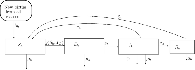
Figure showing the flow of the infection within the human population. The force of infection is denoted by g(S h, I Q) where I Q is a vector containing the reservoir of infected mosquito classes as explained in the text. Natural deaths occur in all classes at rate μ h and births in all classes that enter into the susceptible class occur at the same rate of λ h per human
Table 1 Types of human compartments and their description $$\displaystyle \begin{aligned} \frac{d E_{h}}{d t} &= g(S_{h},\boldsymbol{I}_{Q})-\left(\nu_{h}+\mu_{h}\right)E_{h};{} \end{aligned} $$(2) (3)$$\displaystyle \begin{aligned} \frac{d R_{h}}{d t} &= \sigma_{h}I_{h}-\left(\delta_{h}+\mu_{h}\right)R_{h};{} \end{aligned} $$(4)
with appropriate initial conditions at time t = 0. The model represented by Eqs. (1)–(4) differs from the model in Ngwa and Shu [20] only in the form of the force of infection, g(S h, I Q). The nature of the vector I Q is discussed in Sect. 2.2.
-
2.
The mosquito’s population dynamics based on its gonotrophic cycle. In the mosquito’s population, we shall approach the disease compartmentalization of susceptible, exposed (infected) and infectious in an indirect route that passes via a physiological compartmentalization of the mosquito’s population. That is, we shall base the compartmentalization on the fact that the mosquito undergoes a reproductive cycle called the gonotrophic cycle, so that at any one time each adult female mosquito’s physiological state (well fed with a sugar meal, well nourished with a blood meal, rested after blood feeding, oviposited, nulliparous, mated/fertilized, etc.) on this cycle can be characterized. In what follows, we consider only female adult Anopheles sp mosquitoes since the males only survive on nectar and so, apart from the fact that they help in fertilizing the females, they do not pose any immediate threat to humans. The very nature of the gonotrophic cycle requires that a newly emerged adult female mosquito gets fertilized, searches and takes a blood meal, searches for a resting place and rests, and then searches for a breeding site where she lays eggs to complete the first gonotrophic cycle. Given that she stores the spermatozoa in a special pouch called a spermatheca, she does not need to mate again before the second and subsequent egg laying episodes, [31, 32]. Thus, it is assumed that all subsequent gonotrophic cycles starting from the second constitute only three main steps or locations namely: (i) being at the breeding site (oviposition site), (ii) being at human habitats site as questing mosquitoes and (iii) resting for egg maturation after blood feeding. We can use directed arrows to represent the flow of the mosquitoes as follows: from breeding site → human habitat site for questing for blood meal → Resting for egg development → back to breeding site to lay eggs → human habitat site for questing for blood ⋯. So every egg laying episode is preceded by blood feeding and resting episodes and the cycle is repeated until the mosquito dies of old age if she is not killed at any of the locations. The important point about these gonotrophic cycles is that every successfully completed cycle culminates with the laying of eggs that mature through the mosquito’s metamorphic pathway to eventually increase the population density of the adult mosquitoes. An increase in the adult mosquito’s population density means the availability of more biting mosquitoes that can facilitate the transmission of disease where malaria disease (or any other mosquito borne disease of humans) transmission is also possible. We have captured here a natural process whereby, in the presence of malaria disease, a successful mosquito–human interaction may not only lead to transfer of the infection, but also means an increase in the number of mosquitoes to subsequently take part in the disease transmission process. This is why we have referred to the system studied in this paper as the mosquito–human–malaria interactive framework. To complete the characterization of the framework, we next describe how we can use the length of the gonotrophic cycle as a timer to approximate the chronological age of the mosquito and also identify mosquitoes that were infected early in their adult life and which will most likely be the candidate infectious mosquitoes to humans if they survive subsequent gonotrophic cycles.
-
3.
Embedding the mosquito’s physiological age/disease status in its gonotrophic cycle counter. The density of breeding site mosquitoes is denoted as type B mosquitoes, that of questing mosquitoes as type Q and that of resting mosquitoes as type R as explained in Table 2, and the general framework through which the different classes of mosquitoes relate with each other is shown in Fig. 2. In addition to the identification of the mosquitoes into the three broad types of breeding site, questing and resting mosquitoes, as described in Table 2, we subdivide each type into yet smaller classes indicating disease status, as well as into distinct age stages based on the number of gonotrophic cycles that each mosquito would have had. For example, for a given y ∈{B, Q, R}, we write \(S_{y_{k}}\), k ≥ 1, to denote a susceptible mosquito of type y at reproductive stage k, and \(I_{y_{k,j}}\), k ≥ j ≥ 1, to denote an infected mosquito at reproductive stage k that first picked up the infection at reproductive stage j. By extension, all the parameters of the system also have subscripted notation to capture its association with the particular reproductive stage mosquito. For example, ρ k is the flow rate to the breeding site of susceptible rested mosquitoes at reproductive stage k, \(S_{R_{k}}\), while that of \(I_{R_{k,j}}\) would be ρ k,j. We assume that mosquitoes of all types with a higher gonotrophic cycle counter are older than mosquitoes of the all types but at lower gonotrophic cycle counter. That is, at each cycle k ≥ 2, mosquitoes of type B k are older than mosquitoes of type R k−1, while for each k ≥ 1, we assume that mosquitoes of type B k are younger than mosquitoes of type R k. On the overall scale, we assume that mosquitoes of type B 1 are the youngest while mosquitoes of type R N, N > 1 are the oldest. The gonotrophic cycle counter is thus used as a way to measure the adult mosquito’s chronological age. This is the same compartmentalization as used in [22], but instead of ending the gonotrophic cycle count at 3, we generalize and assume that each adult female mosquito will undergo up to N reproductive cycles represented at each k, for k = 1, 2, ⋯ , N, by the idealization on Fig. 2. Note that N here will be determined by how long a mosquito lives and how often it feeds and lays eggs, during its lifetime. In [23], it is argued that in the wild, based on a conceptualization of days and activities in the adult mosquito’s life for the possible number of times the mosquito lays eggs during its reproductive life, the number N can be as large as N = 4 for a mosquito that lives for 24 days. The detailed definition of each of the compartments is shown in Table 3. The parameters of the system that we shall derive are shown in Table 4. In Fig. 3 we display the flow chart for a mosquito–human interactive system where each mosquito can undergo up to N complete gonotrophic cycles. That is, for a disease-free system in which we have mosquitoes interacting with humans and reproducing through the mechanisms explained above. This is the conceptualization of the system studied in [23]. Counting the number of compartments for this disease-free system gives 3N mosquito compartments. In the presence of malaria, the number of compartments in the mosquito populations grows considerably and so it will be important to carefully examine how each of these compartments come about and how they contribute to the general mosquito–human–malaria interactive framework.
Fig. 2 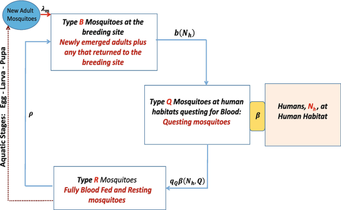
Idealization of mosquito’s movement at each gonotrophic cycle. Breeding site mosquitoes are attracted to human habitats at rate b(N h), where they become questing mosquitoes of type Q. Mosquitoes of type Q interact with humans N h. Upon successful acquisition of a blood meal through the interactive exposure rate β(N h, Q), the mosquitoes of type Q become resting mosquitoes of type R. After the requisite resting period, the mosquitoes of type R that survive migrate again to the breeding site at rate ρ where they lay eggs that eventually contribute to the new adult mosquito population through the new adult mosquitoes’ compartment. Upon successful arrival at the breeding site to lay eggs, the returned mosquitoes become breeding site mosquitoes of type B but with a higher gonotrophic cycle counter. q Q is the probability of successfully completing a blood feeding episode to move into the resiting and egg maturation phase
Fig. 3 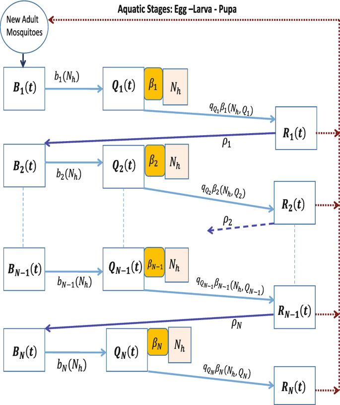
Idealization of mosquito’s movement according to gonotrophic cycles showing the mosquito only flows. Breeding site mosquitoes at reproductive stage k are attracted to human habitats at rate b k(N h), where they become questing mosquitoes of type Q k. Mosquitoes of type Q k interact with humans N h with exposure rate β k(N h, Q k). Upon successful acquisition of a blood meal through the interactive exposure rate \(q_{Q_{k}}\beta _{k}(N_{h},Q_{k})\), the mosquitoes of type Q k become resting mosquitoes of type R k. After the requisite resting period, the mosquitoes of type R k that survive migrate again to the breeding site at rate ρ k where they lay eggs that eventually contribute to the new adult mosquito population through the new birth term. Upon successful arrival at the breeding site to lay eggs, the R k mosquitoes become breeding site mosquitoes of type B k+1 and the cycle continues. The Mosquitoes of type R at reproductive stage N, R N, lay their final batch of eggs and then die of old age and no longer enter the cycle
Table 2 Types of mosquitoes and their description Table 3 The compartmentalization of the mosquito vectors as a function of reproductive stages k and j, for k = 1, 2, 3, ⋯ , N and j = 1, 2, 3, ⋯ , N, as well as according to disease status: infected, I, or non-infected S. Only mosquitoes of type Q can interact with humans and so the disease can be transmitted from a human to a mosquito and vice versa only through mosquitoes of type Q. Furthermore, only infected mosquitoes of type \(I_{Q_{k,j}}\) with k − j ≥ 2 can be infectious to humans Table 4 The parameters of the system and their quasi-dimension. Time in days (T), Bites (b), Vectors (V). All parameters are non-negative. Quasi-dimension of a parameter is its unit of measurement


From the compartmentalization adopted, only mosquitoes of type Q interact with humans so that the infection can pass from humans to mosquitoes only through the interaction of type S Q mosquitoes interacting with either infectious humans of type (I h) or the mildly infectious recovered and partially immune humans of type (R h). Figure 4 shows the full flow of the infection within the mosquito population for a mosquito–human–malaria interactive framework where each mosquito can undergo up to a maximum of three gonotrophic cycles. The figure clearly indicates the points where the infection can be passed from the human population into the mosquito population. The first column of compartments, comprising only the S ∗ variables constitute the material shown in Fig. 3. New infections can pass from mosquitoes to humans only through an interaction between a susceptible human of type (S h) with an infected questing mosquito that is infectious. That is, mosquitoes of type \(I_{Q_{k,j}}\), k ≥ j + 2. The insistence that k ≥ j + 2 ensures that we capture the minimum extrinsic incubation period; that is, the minimum time period required by an infected mosquito for the disease to mature to a level that the mosquito can now be infectious to humans. Here, we are assuming that each mosquito will spend approximately the same length of time to complete each gonotrophic cycle. Although this can be an unrealistic assumption, given the perilous environment in which the mosquito must live and search for blood meals, we continue to use 2 as the minimum number of gonotrophic cycles whose cumulative time length is equivalent to the time lapse required for the infection to mature in the mosquito.Footnote 2

The full mosquito–human–malaria interactive framework for n = 3 showing the flow of infection and movement of mosquitoes within the mosquito population. In the mosquito–human–malaria interactive framework used in this paper, only mosquitoes of type Q can interact with humans and infection can pass from human to mosquito only through the successful interaction between a susceptible mosquito of type Q, at reproduction stage k, \(S_{Q_{k}}\), and an infectious human. This is the source of the new infected mosquito compartment \(I_{R_{k,k}}\), k = 1, 2, 3 shown. Each new infected mosquito compartment starts a new branch of infected mosquitoes’ path that eventually contribute to the source of infectious mosquitoes within the mosquito population as explained in the text. Contributions into the new adult mosquito pool after each blood meal episode by a fed and rested mosquito of type R are shown by the brown dotted lines. Additional infection of already infected mosquitoes is not considered
The total adult mosquito population implicated in the model constitutes only those anthropophilic mosquitoes that consistently seek for blood meals within the human population. If N v is the total mosquito population size, then N v = N R + N Q + N B where N R, N B and N Q are respectively the sizes of the total resting, breeding site and questing mosquitoes, given by
where \(S_{*_{k}}\) and \(I_{*_{k,j}}\) for ∗ ∈{R, B, Q}, are as defined in Table 3. In this formulation, k tracks the reproductive stage of the adult mosquito, and hence the age, meanwhile j tracks the reproductive stage at which the adult mosquito was first infected with the malaria parasite.
Taking into consideration the full breadth of possible number of gonotrophic cycles and considering that disease dynamics adds to the complexity of the problem, we believe that it will be informative to have an idea of the size of the system. We already know that in the human population there are four compartments representing disease status with two of these compartments potentially infectious to mosquitoes. This gives us up to about a 50% chance of having an infectious human compartment in the modelling framework. We now work out the size of the system by calculating the total number of possible compartments in the mosquito population within the current framework. We state and prove the following result:
Lemma 1 (On the Size of the System)
Let there be given a mosquito–human–malaria dynamical system interactive framework whereby the mosquito can undergo up to N gonotrophic cycles during its entire reproductive life. Assume that at each gonotrophic cycle, there are three possible compartments: Q, B and R representing the three phases of breeding, questing and resting as conceived above. If in addition a mosquito in each of the compartments can be in any one of the disease states of infected (infectious) or susceptible, and if \(\mathcal {M}(N)\) is the total number of mosquito compartments for the system, then \(\mathcal {M}(N) = \frac {N}{2}(5+3N)\) where N is the maximum number of gonotrophic cycles possible for each adult mosquito.
Proof
At gonotrophic cycle one, we have the three starting susceptible compartments \(S_{B_{1}}\), \(S_{Q_{1}}\) and \(S_{R_{1}}\). At this cycle, a questing mosquito can become infected to give the additional infected resting compartment \(I_{R_{1,1}}\). This gives a maximum number of 4 possible compartments at reproductive or gonotrophic cycle 1. The two possible R compartments from gonotrophic cycle 1 each give rise to three compartments at gonotrophic cycle 2 as follows: vectors from the susceptible compartment \(S_{R_{1}}\) migrate to the breeding site as susceptible vectors of type B at gonotrophic cycle 2, \(S_{B_{2}}\) which eventually follow the mosquito behavioural pattern to produce \(S_{Q_{2}}\) and \(S_{R_{2}}\). The infected resting mosquitoes, \(I_{R_{1,1}}\) migrate to the breeding site to become infected breeding site mosquitoes at reproductive stage 2, \(I_{B_{2,1}}\). These, also following the mosquito’s behavioural pattern, produce \(I_{Q_{2,1}}\) and \(I_{R_{2,1}}\). The susceptible questing mosquitoes at reproductive stage 2 can become infected to produce infected resting mosquitoes at reproductive stage 2; \(I_{R_{2,2}}\).
All mosquitoes that enter the next stage as infected mosquitoes do not add additional new infections into the mosquito sub-system. So we have a total of only 7 mosquito compartments at reproductive stage 2. Thus in general, each R compartment at the current level will produce three new compartments in the next level with a possibility of generating one additional new R compartment at that new level whenever new infections pass from the humans into the mosquito population. We thus have the sequence (c k)k≥1 where each c k = 3k + 1 is the number of compartments at the k-th gonotrophic cycle. Thus, the total number of compartments after all N gonotrophic cycles is
as required. See illustration of compartment count in Fig. 5 for N = 4. \(\square \)

Illustration of the gonotrophic cycle flow chart for N = 4. The cycles are demarcated with dashed lines. At gonotrophic cycles 1, 2, 3 and 4 there are respectively 4, 7, 10 and 13 possible mosquito compartments. So that at gonotrophic cycle n there will be 3n + 1 mosquito compartments
2.2 The Exposure, Flow, Contact, Infectivity and Recruitment Rates
-
1.
The mosquito flow rate from breeding site to human habitat sites. The flow rate from breeding site to human habitat is derived by considering the blood factor index for the mosquito and accounting for those mosquitoes that eventually choose to take a blood meal from the human population. If a k is the rate of flow of vectors from breeding site to vertebrate habitat sites, then a k is weighted by the quantity \(\frac {N_{h}}{N_{h}+\kappa }\) where κ is a measure of the existence of an alternative blood source for the mosquito [22], so that \(b_{k}(N_{h}) = a_{k}\frac {N_{h}}{N_{h}+\kappa }\) is a measure of the effective rate of flow of breeding site mosquitoes at reproductive stage k to the human habitats. It is understood that the fraction \(1-\frac {N_{h}}{N_{h}+\kappa }\) of a k constitutes that fraction that searches for blood meals from non-human sources.
-
2.
The flow rate of resting/rested vectors to the breeding site. After the acquisition of a blood meal, the adult female mosquito finds a suitable resting place where she rests for her eggs to mature. After a successful completion of the rest period, the rested mosquito that is ready to lay her eggs must migrate to the breeding site. Two states of vectors are considered and their flow rates differentiated accordingly: The flow rate to the breeding site of susceptible rested mosquitoes at reproductive stage k, denoted by ρ k and the flow rate of rested infected adult mosquitoes at reproductive stage k, that were first infected (with malaria) at reproductive stage j, ρ k,j. A resting mosquito at reproductive stage k that successfully arrives at the breeding site to lay its eggs shall become a breeding site mosquito now at reproductive stage k + 1.
-
3.
Exposure rate of humans to questing mosquitoes. As in [22], the exposure rate of humans of a general type, say Y h, Y ∈{S, E, I, R}, when interacting with questing mosquitoes of type Q at reproductive stage k, represented generally as \(X_{Q}\in \{S_{Q_{k}},I_{Q_{k,j}}\}\), is denoted β k and takes the form \(\beta _{k}(Y_{h},X_{Q})=\frac {b_{Q_{k}}X_{Q}Y_{h}}{N_{h}}\) where \(b_{Q_{k}}\) is the human biting rate of the mosquito at reproductive stage k and N h is the total human population available to the questing mosquitoes. To be specific, if X Q is a susceptible questing mosquito at reproductive stage k, \(S_{Q_{k}}\), then we have \(\beta _{k}(Y_{h},X_{Q})= \beta _{k}(Y_{h},S_{Q_{k}})\). If the questing mosquito is already infected, the infected mosquito is identified with its current reproductive stage and the reproductive stage where infection first took place through the double subscript notation so that \(X_{Q} = I_{Q_{k,j}}\), a questing mosquito of type I at reproductive stage k, that was first infected at reproductive stage j and \(\beta _{k}(Y_{h},X_{Q}) = \beta _{k}(Y_{h},I_{Q_{k,j}})\). This double subscript notation allows us to track the chronological age of the mosquito through its gonotrophic cycles counter as well as from when it first picked up the infection from the human. This way, the incubation period of the disease within the mosquito population is implicitly built into the modelling framework by assuming that the equivalent of at least two gonotrophic cycles episodes must elapse from time of first infection to the time when the questing mosquito is infectious to humans.
-
4.
Effective contact rates. We consider two levels of having an effective contact between the humans and the mosquitoes: In the first instance, we consider an interactive contact that is effective in the sense that the contact leads to the transfer of infection from the human to the mosquito or from mosquito to human, and in the second instance, we consider a contact which is effective in the sense that the mosquito ingests enough blood to be able to satisfy its reproductive need. In the current formulation, we assume that when a mosquito engages in an interaction and fails to get the required blood meal, it is assumed killed in the process. In a more realistic setting, we would consider a case where a fraction of the mosquitoes that fail to get the required blood meal lives to try again as many times as it is required. We do not consider this in the present formulation, but only the following possibilities:
-
(a)
The questing mosquito at reproductive stage k that successfully takes a blood meal with probability \(q_{Q_{k}}\) shall become a resting mosquito of type R at reproductive stage k. So, it fails to take the blood meal upon trying with probability \(1-q_{Q_{k}}\) which, in this case, is the probability of certain death. Two types of resting mosquitoes are identified in this work: susceptible resting mosquitoes at reproductive stage k whose density is denoted by \(S_{R_{k}}\) and infected mosquitoes at reproductive stage k that first picked up the infection at reproductive stage j, whose density is denoted by \(I_{R_{k,j}}\).
-
(b)
A susceptible questing mosquito at reproductive stage k that successfully takes a blood meal with probability \(q_{Q_{k}}\) from an infectious human and also succeeds in picking up an infection from human with probability \(p_{hQ_{k}}\) shall become an infected resting mosquito and the time counter to measure the length of the period of it being infected starts from the counter of the reproductive stage where it first got infected. So, for emphasis, we use the notation \(I_{R_{k,j}}\) to denote the density of infected resting vectors at reproductive stage k that first picked up the malaria infection at reproductive stage j.
-
(c)
An infectious questing mosquito at reproductive stage k that was first infected at reproductive stage j that successfully takes a blood meal from a susceptible human with probability \(q_{Q_{k}}\) and also transfers the infection to the human with probability \(p_{Q_{k}h}\) shall become a resting infected mosquito at reproductive stage k that was first infected at reproductive stage j.
-
(d)
Where the mosquito or human is already infected, further infection is not considered. That is, we do not consider super-infection. However, every successful blood meal episode leads to oviposition by the mosquito which in turn leads to the eclosion of new adult mosquitoes that go to increase the total adult mosquito population. Where infection is present and not transferred, the probability of failure to transfer is \(1-p_{hQ_{k}}\) or \(1-p_{Q_{k}h}\), respectively.
-
(a)
-
5.
Infectivity of humans to mosquitoes. The incubation period of the disease in humans, when caused by Plasmodium falciparum, has been estimated to be about 12 (9–14) days. This incubation period can be longer for other Plasmodium species of the parasite [27]. So, from the time of first infection with Plasmodium falciparum parasites, it takes about 12 days for the disease to develop in the human to the level where the human can become infectious to the mosquito. This fact is captured in the model by including a compartment of the human population wherein the humans are exposed to the infection but not yet infectious to mosquitoes. After the incubation period, the human can then become infectious where the rate of onset of infectiousness is inversely proportional to the residence time in the incubation phase. Infectious humans can recover without gain of immunity to join the susceptible class, or they can recover from clinical illness with a substantial gain of immunity to enter a partially immune class wherein members of that class are immune to clinical symptoms of malaria but are still mildly infectious to mosquitoes. This phenomenon of incomplete immunity permitting disease transmission has been known for some time now [2,3,4], and represents one of the main reasons why malaria eradication is difficult, among others; the reservoir of infection in the human population includes both symptomatic and asymptomatic immune carriers. To derive the expression for the infectivity of the human to the mosquito, we simply multiply the exposure rate of the mosquitoes to human, as derived above, with the probability of an effective contact between the questing susceptible mosquito at reproductive stage k, \(q_{Q_{k}}\) with the probability of the infectious human infecting the reproductive stage k questing mosquito, \(p_{hQ_{k}}\) if the human is from class I h and \(\tilde {p}_{hQ_{k}}\), if the human is from class R h. Therefore, if f k(S Q, I h, R h) is the force of infection for the stage k questing mosquitoes, that is the rate of change of new infections into reproductive stage k questing mosquitoes, then
$$\displaystyle \begin{aligned} \begin{array}{rcl} f_{k}(S_{Q_{k}},I_{h},R_{h})=p_{hQ_{k}}q_{Q_{k}}\beta_{k}(I_{h},S_{Q_{k}}) + \tilde{p}_{hQ_{k}}q_{Q_{k}}\beta_{k}(R_{h},S_{Q_{k}}){}. \end{array} \end{aligned} $$(7)These new infections will enter the \(I_{R_{k,k}}\) compartment as a starting point of each new infection entering the mosquito population. Formula (7) captures the fact that asymptomatic immune malaria carriers can be infective to mosquitoes; however, we must expect that \(p_{hQ_{k}}>\tilde {p}_{hQ_{k}}\) to capture the fact that infectivity of the type R h humans is less than that of the I h humans and that the reservoir of infection in the human population includes both symptomatic and asymptomatic immune malaria carriers.
-
6.
Infectivity of mosquitoes to humans. The incubation period of the disease in mosquitoes can be as low as 10 days, [5, 27, 29] but can be made shorter in higher temperatures [5]. The length of the incubation period in mosquitoes can also be different for different species of the malaria parasite. So, from the moment the mosquito first picks up the infection we have to wait at least 10 days for the disease to mature in the mosquito before the mosquito can bring back the infection into the human population. During these 10 days, the reproductive cycle activities of blood feeding and egg laying continue as they will still continue after the 10 days incubation period. We implicitly model the incubation period of the disease in the mosquito population by requiring that an equivalent time length, measured by a cumulative time lapse equivalent to the length of at least two gonotrophic cycles, be completed by the mosquito before it can become infectious to the human. Thus, a questing mosquito at gonotrophic cycle k, that picked up the infection as a questing mosquito at gonotrophic cycle j, \(I_{Q_{k,j}}\), is considered infectious to humans only if k − j ≥ 2. Therefore only older mosquitoes that were infected much earlier in their gonotrophic cycle count, and which have undergone at least two gonotrophic cycle counts since first infection, shall be infectious to humans.
From the forgoing, we deduce that not all infected mosquito compartments contain infectious mosquitoes. So, it will be informative to work out the size of the reservoir of infection (ROIV ) in the mosquito population. Let \(M<\mathcal {M}(N)\) be the number of compartments containing infectious questing mosquitoes. We seek to quantify the number of infectious questing mosquito compartments, \(I_{Q_{k,j}}\), 3 ≤ k < N, 1 ≤ j ≤ N − 2, k ≥ j + 2. We can state and prove the following result on the actual size of M(N) for a dynamical system where the total number of reproductive cycles possible is N.
Lemma 2 (On the Number of the Infectious Questing Mosquito Compartments)
Consider a system where the total number of gonotrophic cycles is N. Suppose that an infected mosquito at reproductive stage k that was first infected at reproductive stage j, \(I_{Q_{k,j}}\) , requires at least two gonotrophic cycles before it can become infectious to humans. If M is the number of infectious compartments in the vector population, then \(M=\frac {1}{2}(N-1)(N-2)\).
Proof
If each infected mosquito requires at least two gonotrophic cycles from time of first infection to the onset of infectiousness, then a mosquito that picked up the infection in its first gonotrophic cycle will become infectious to humans as from its third gonotrophic cycle. We thus have \(I_{Q_{k,1}}\), for k = 3, 4, 5, ⋯ , N, giving a total of N − 2 infectious questing compartments. Next, a mosquito that picked up the infection during its second gonotrophic cycle will become infectious to humans as from the 4th gonotrophic cycle. We thus have in this case \(I_{Q_{k,2}}\), for k = 4, 5, ⋯ , N, giving a total of N − 3 infectious questing compartments. Continuing in this way, we find that a mosquito that picked up the infection during its N − 2 gonotrophic cycle will become infectious at gonotrophic cycle N, giving only one infectious questing compartment, \(I_{Q_{N,N-2}}\). Questing mosquitoes that pick up the infection either at the N − 1 or N gonotrophic cycles shall die before the maturation of the disease, and so this class of infected vectors will not play a part in the spread of the infection, although they will contribute to the size of the total mosquito population. Thus the total number of infectious questing compartments can be obtained by summing up the number of compartments associated with infectious questing and is
$$\displaystyle \begin{aligned} \begin{array}{rcl} M (N) = \sum_{i=1}^{N-2}i = \frac{1}{2}(N-2)(N-1),{} \end{array} \end{aligned} $$(8)as required. \(\square \)
Remark 1 (Generalization of Lemma 2)
We can attempt a generalization of the result of Lemma 2 as follows: If n is the number of cycles that must elapse from time of first infection to time of onset of infectiousness of the mosquito, then from the biology of the Anopheles mosquito and the incubation period of the malaria infection in the mosquito, we deduce that n ≥ 2, every thing being equal. Thus in this general case, M the number of infectious compartments would be given by \(M= \sum _{i=1}^{N-n}i = \frac {1}{2}(N-n)(N-n+1), ~ n\geq 2\). We must conclude, therefore, that M so calculated by Lemma 2 is the largest realistic integer that may be used as an indicator of the size of the number of infectious questing mosquito compartments in this framework.
The importance of Lemma 2 lies in the fact that we can combine its results with those of Lemma 1 to work out the probability of finding an infectious mosquito compartment in the entire mosquito sub-system, which result can be used to work out the chances of passing the infection from mosquito to human. In trying to understand the issue of chances of finding an infected mosquito in the system as well as the number of possible mosquito compartments of the system, we must settle two important parameters of the compartmental modelling process: (i) The number of compartments in the mosquito demographic framework and (ii) the length of the incubation period of the disease in a mosquito as captured by gonotrophic cycle count. Bearing these two facts it mind, we start by noting that the total number of mosquito compartments that eventually arise will be linked to the number of compartments originally conceived for the mosquito demographics model framework at each gonotrophic cycle. In the derivation of the result of Lemma 1, the demographic model has three compartments to capture the breeding, questing and resting phases of the adult mosquito’s reproductive life and shown in Fig. 2. It is possible to adjust the demographic model’s compartmentalization to include other important steps in the adult mosquito’s life such as searching for first sugar meal after adult eclosion, swarming, mating, first rest after mating, etc. This will drastically increase the number of compartments in the demographic model’s compartmentalization framework. However, we do not think that the chances of finding an infected mosquito compartment in the system are equivalent to the probability of finding an infectious mosquito, unless the assumption can be made that the proportion of mosquitoes within each of the defined compartments are same or close to being the same. In the second instance, we also note that the number of compartments containing infected and infectious mosquitoes that shall be found in the system will be determined by a parameter equal to the number of gonotrophic cycles whose cumulative length of time is equivalent to the length of the incubation period of the disease in the mosquitoes. In the derivation of the results of Lemma 2, this number was set to 2, and is the number used in this manuscript, but was later generalized to n ≥ 2 as in Remark 1. We can now state and prove the following result:
Lemma 3 (On the Probability of Finding an Infectious Mosquito Compartment)
Let there be given a mosquito–human–malaria dynamical system interactive framework in which the mosquito can undergo up to a maximum of N gonotrophic cycles during its entire reproductive life. Assume that to complete one gonotrophic cycle, the mosquito must pass through m distinct compartments where only one of these compartments represent interaction with humans and through which infection can pass into (or out of) the mosquito population. Let \(\mathcal {M}_{m}(N)\) be the total number of compartments that this system can generate, and M n(N) the total number of infectious mosquito compartments in the system, where n is the number of cycles that must elapse from time of first infection to time of onset of infectiousness of the mosquito. Let P m,n(k) be the probability of finding an infectious compartment at gonotrophic cycle k. Then,
$$\displaystyle \begin{aligned} \begin{array}{rcl} P_{m,n}(k) = \left\{\begin{array}{ll}0,&0\leq k\leq n;\\ \frac{(k-n)(k-n+1)}{k(mk +m+2)},& n\leq k\leq N,\end{array}\right. \mathit{\mbox{ and }}\lim_{k\to\infty}P_{m,n}(k)= \frac{1}{m}{} \end{array} \end{aligned} $$(9)Proof
Given that of the m compartments, infection can pass through only one of them, only one new infected mosquito compartment can be produced at each gonotrophic cycle level. Following the same argument as used in Lemma 1, we find that given m compartments at the start, at gonotrophic cycle k we have c k = mk + 1 compartments and so the total for all cycles, \(\mathcal {M}_{m}(N)\) is given by
$$\displaystyle \begin{aligned} \begin{array}{rcl} \mathcal{M}_{m}(N) = \sum_{k=1}^{N}c_{k}=\sum_{k=1}^{N}(mk+1) = \frac{1}{2}N(mN+m+2). \end{array} \end{aligned} $$(10)From Remark 1 we have that if M n(k) is the number of infected and infectious compartments in the system at gonotrophic cycle k, where we require at least n gonotrophic cycles before infected vectors can become infectious, then
$$\displaystyle \begin{aligned} \begin{array}{rcl} M_{n}(k) = \left\{\begin{array}{ll}0,&0\leq k\leq n;\\ \frac{1}{2}(k-n)(k-n+1),& n\leq k \leq N.\end{array}\right. \end{array} \end{aligned} $$(11)Therefore from standard probabilistic arguments we have that,
$$\displaystyle \begin{aligned} \begin{array}{rcl} P_{m,n}(k) = \frac{M_{n}(k)}{\mathcal{M}_{m}(k)}= \left\{\begin{array}{ll}0,&\displaystyle 0\leq k\leq n;\\ \frac{(k-n)(k-n+1)}{k(mk +m+2)},&\displaystyle n\leq k\leq N,\end{array}\right. \mbox{ and }\lim_{k\to\infty}P_{m,n}(k)= \frac{1}{m} \end{array} \end{aligned} $$as required. \(\square \)
So while the probability of finding an infected compartment increases with increasing number of gonotrophic cycles, the rate of increase is decreasing. So we should not expect to get more infectious compartments from the system just by allowing the mosquitoes to undergo more gonotrophic cycles. We conjecture that this is linked to the fact that the infection must mature in the mosquito before being available for transmission as well as to the fact that the “bottleneck” requiring that the infection must pass through the questing mosquito compartment limits the possibilities. In Fig. 3, we illustrate the behaviour of the probability of finding an infectious mosquito compartment in the system for different values of m and n. The shape of the graph is similar for various m and k values as described in formula (9).
By considering the limiting behaviour of the probability P m,n(k), we deduce that the chances of finding an infectious compartment in the human population are higher (up to 50%) than that of finding an infectious compartment in the mosquito population (less than 33% for the case m = 3 and 25% for the case m = 4). This information may be useful in determining the infectivity of the biting mosquito if the assumption is that the population sizes of mosquitoes in these compartments are about the same. Formula (9) shows that even though the length of the incubation period is important in determining when a compartment is infectious, this parameter’s effect, once set, diminishes as the number of gonotrophic cycles increases. On the other hand, the parameter m is more important if we make the assumption that the population of mosquitoes within each mosquito compartments is about the same. However, if the population of mosquitoes in the infectious classes is smaller than the population size in the other compartments, then the importance of m is diminished. Perhaps we should not expect better results with more compartments in the demographic compartmentalization framework, but more on the distribution of the mosquitoes within these compartments. In what follows we continue to use the case m = 3 and n = 2 (Fig. 6).
Fig. 6 
The probability, P m,n(k), of finding an infectious mosquito compartment in the entire mosquito–human system is plotted as a function of the number of gonotrophic cycles reached for the cases (m, n) = (3, 2) and (3, 4), illustrated by the black and red solid curves, and also the cases (m, n) = (4, 2) and (4, 4), illustrated by the black and red dashed curves. The probability changes very rapidly in a narrow range of values of gonotrophic cycles. As the number of gonotrophic cycles increases further, the probability approaches \( \frac {1}{3}\) for the cases when m = 3 and illustrated by the solid light pink line, and it approaches \( \frac {1}{4}\) when m = 4 as illustrated by the dashed light pink line. If the number of compartments in the demographic model framework is increased, the chances of finding an infected mosquito compartment reduce. This result is only as important as the assumption that in the compartmentalization choices, the proportion of mosquitoes in the various compartments will be close or as close to being the same
The number of infectious mosquito compartments may be displayed in a vector \(\boldsymbol {I}_{Q}\in \mathbb {R}^{M}\) where M is given by Eq. (8) and \(\boldsymbol {I}_{Q} = (I_{Q_{k,j}},3\leq k\leq N, ~ 1\leq j\leq N-2, k>j)\in \mathbb {R}^{M}\). We shall refer to I Q as the reservoir of infection vector (ROIV). We now use the entries of ROIV to derive the force of infection in the human population. Let g(S h, I Q) be the force of infection in the human population. Then g is modelled by considering all those interactions between susceptible humans S h and all the infected and infectious questing mosquitoes found in the mosquito’s ROIV. As mentioned above, employing the convention that each infected mosquito must go through at least two gonotrophic cycles before becoming infectious will implicitly build the incubation period of the disease into the mosquito population. The force of infection in the human population is therefore a sum over all those human-mosquito effective contacts, \(\beta _{k}(S_{h},I_{Q_{k,j}})\), that lead to acquisition of blood meal with probability \(q_{Q_{k}}\) together with the probability of transferring the infection to the human with probability \(p_{Q_{k}h}\). Thus multiplying and summing up we have the expression
$$\displaystyle \begin{aligned} \begin{array}{rcl} g(S_{h},\boldsymbol{I}_{Q}) = \sum_{j=1}^{N-2}\sum_{k=j+2}^{N}p_{Q_{k}h}q_{Q_{k}}\beta_{k}(S_{h},I_{Q_{k,j}}). {} \end{array} \end{aligned} $$(12)The force of infection so constructed takes into consideration all those infected and infectious anthropophilic mosquitoes that are participating actively in the dynamics.
-
7.
The rate of recruitment of new adult mosquitoes. The actual existence of mosquitoes to continue to the next generations depends on the fact that mosquitoes of type R find suitable breeding sites to lay their eggs. It may be that a mosquito will choose a particular breeding site over another depending on several factors that could include the absence of predators, presence of other larvae at that breeding site or proximity from the resting place. Thus, the relationship between the mosquitoes of type R and the newly emerging adults cannot simply be assumed to be a linear response. This perhaps necessitates an assumption that the adult mosquito eclosion rate is density dependent. Some sources, for example [7], use a delay modelling argument, to derive a formula for the rate of emergence of new adults in a delayed differential equation framework. Others, see for example [1, 12], approach the problem of modelling the rate of new adult mosquito eclosion by including at least one (or more) state variable to represent the aquatic stages of the mosquito and then evoke the idea that the limitation of the carrying capacity of the aquatic pond will introduce competition within the aquatic stages of the mosquito’s population as a source of nonlinearity and density dependence on the dynamics. Here, we simply assume that the net effect of the activities of the adult mosquitoes of type R is to contribute to the density of adult mosquito in the next generation through a birth term at a rate whose size is quantified by the birth rate function \(\lambda _{R}:[0,\infty )\to \mathbb {R}\). The function λ R, so described and fixed, in general, is assumed to depend in a nonlinear way on the size of the mosquitoes of type R that eventually survive the resting phase and then are in a position to lay eggs when they return to the breeding sites. Here, we assume that the form of the real valued function λ R must satisfy desired properties, which among others, will guarantee the continued existence of a buoyant adult mosquito population so that the growth dynamics of the mosquitoes, in the absence of malaria infection, is internally stable from a mathematical and physical stand point. We write down the following definition:
Definition 1 (Recruitment Functions)
For the sake of mathematical and biological realism, a function \(\lambda _{R}: [0,\infty ) \rightarrow \mathbb {R}\) is a suitable recruitment rate function if λ R is smooth and in addition should satisfy the following:
-
(1)
λ R(0+) > 0, where \(\lambda _{R}(0_+) = \lim _{x \rightarrow 0^+} \lambda _{R}(x).\)
-
(2)
\(\lambda _{R}^{\prime }(x) \) exists with \(\lambda _{R}^{\prime }(x) < 0,~~\forall x \geq 0.\)
-
(3)
\(\lim \limits _ {x\rightarrow +\infty } \lambda _{R} (x) < \lim \limits _ {x\rightarrow 0^+}\lambda _{R} (x).\)
-
(4)
The function xλ R(x) is continuously differentiable, bounded above and unimodal so that there exists \(\hat {x}>0\) such that for \(0<x<\hat {x}\), xλ R(x) is strictly monotone increasing and for \(x>\hat {x}\), xλ R(x) is strictly monotone decreasing.
Remark 2 (Consequences of the Assumptions on λ R)
Each of the conditions considered in the above has consequences on the expectations of the behaviour of the function λ R as follows:
-
(a)
Condition (1) ensures that λ R is non-negative for small values of its argument and represents the rate of production of new x, per x, per time so that the quantity xλ R(x) represents the net rate of production of new x per time.
-
(b)
Condition (2) ensures that λ R is a monotone decreasing function of its argument.
-
(c)
Condition (4) ensures that xλ R(x) has a positive maximum value given by \(\hat {x}\lambda _{R}(\hat {x})\), where \(\hat {x}\in [0,\infty )\) satisfies the equation \(\lambda _{R}(\hat {x}) + \hat {x}\lambda _{R}^{\prime }(\hat {x})=0\).
-
(d)
Condition (3) ensures that the equation x ′(t) = x(t)λ R(x(t)) − μ v x(t), where μ v > 0 can be seen as a natural death rate parameter per x, and which represents a form of the equation for the dynamics of mosquitoes in the absence of infection, has a non-zero steady state solution x ∗ satisfying the equation x ∗ λ R(x ∗) − μ v x ∗ = 0 which is stable. Observe that such a non-zero steady state, x ∗, will be found through the formula \(x^{*} = \lambda _{R}^{-1}(\mu _{v})\), which exists and is positive owing to the monotonicity of λ R whenever limx→∞ λ R(x) < μ v < λ(0+).
-
(e)
All conditions put together ensure the existence of a carrying capacityFootnote 3 L such that for x < L, \(\frac {d x}{dt} > 0\) and thus the population x(t) is increasing with time and for x > L, \(\frac {d x}{dt} < 0\) and thus x(t) is decreasing with time t. Examples of birth functions found in the biological literature that satisfy (1)-(4) may be found in Brännström and Sumpter [6].
In a general analysis, we may wish to investigate the effect and outcome of different birth functions on the dynamics of the system.
In the context of the generalized model presented in this paper, mosquitoes of type R can be in one of two states: Susceptible mosquitoes of type R at reproductive stage k; \(S_{R_{k}}\), or infected mosquitoes of type R at reproductive stage k that were first infected at reproductive stage j; \(I_{R_{k,j}}\). Each of these do contribute to the next generation of adult mosquitoes upon successful completion of resting period.Footnote 4 To differentiate the contributions, from each type R mosquito, to the next generation of the new adult mosquito’s population, we write \(\lambda _{k}(S_{R_{k}}) = \lambda _{S_{R_{k}}}(S_{R_{k}})\) and \(\lambda _{k,j}(I_{R_{k,j}}) = \lambda _{I_{R_{k,j}}}(I_{R_{k,j}})\). Then, we set \(\lambda _{0_{k}}=\lambda _{k}(0+) = \lim _{S_{R_{k}}\to 0}\lambda _{S_{R_{k}}}(S_{R_{k}})\) and \(\lambda _{0_{k,j}}=\lambda _{k,j}(0+) = \lim _{I_{R_{k,j}}\to 0}\lambda _{k,j}(I_{R_{k,j}})\). To be specific, we use a simple density dependent form of the birth function that satisfies conditions (1)–(4) above and define, at each reproductive stage k the linear functions
$$\displaystyle \begin{aligned} \begin{array}{rcl} \lambda_{k}(S_{R_{k}}) = \lambda_{0_{k}}\left(1-\frac{S_{R_{k}}}{L_{k}}\right), ~\mbox{ and }\lambda_{k,j}(I_{R_{k,j}}) = \lambda_{0_{k,j}}\left(1-\frac{I_{R_{k,j}}}{L_{k,j}}\right){} \end{array} \end{aligned} $$(13)where \(\lambda _{0_{k}}>0\) and \(\lambda _{0_{k,j}}>0\) are constants measuring the limiting size of the oviposited egg cluster by rested mosquitoes at reproductive stage k when population numbers of those mosquitoes are small, and L k and L k,j are parameters linked to the environmental carrying capacityFootnote 5 for stage k vectors of type R. The form of λ k or λ k,j prescribed by Eq. (13) can go negative when \(S_{R_{k}}> L_{k}\) or \(I_{R_{k,j}}> L_{k,j}\) which will then show that for these values of \(S_{R_{k}}\) and \(I_{R_{k,j}}\), the rate of oviposition is negative signifying declining population numbers. This behaviour actually represents a realistic mathematical idealization of the population growth process and so represents a good starting point in considering nonlinear dynamics for the mosquito’s population. Other advantages in using these forms are that they are linear and could serve as the first linear approximation for any nonlinear function that satisfies conditions and assumptions of Definition 1. The main reason we continue to use the linear birth rate is because of mathematical tractability of the resulting equations based on this linear birth rate model. More nonlinear functions have been used in malaria modelling. See, for example, [17, 21].
The functional response of the resting mosquitoes in contributing to the general mosquito population size will be determined by the way in which we model inter-specific competition (if any) between the members of the rested/egg laying mosquitoes. Two formulations are possible:
-
(a)
In the first instance we can assume that λ k and λ k,j are a functions of the total size of the resting mosquitoes N R where N R is given by (5) so that we have the expression
$$\displaystyle \begin{aligned} \begin{array}{rcl} \mbox{New adults} &\displaystyle =&\displaystyle \sum_{k=1}^{N}\rho_{k}\lambda_{k}(N_{R})S_{R_{k}} + \sum_{j=1}^{N}\sum_{k=j}^{N}\rho_{k,j}\lambda_{k,j}(N_{R})I_{R_{k,j}}.{} \end{array} \end{aligned} $$(14) -
(b)
In the second instance, we assume that each mosquito specifically lives a separate life style so that we can consider a rate of recruitment of new adult mosquitoes into the system to come from contributions from the independent classes of resting mosquitoes and write down an expression of the form
$$\displaystyle \begin{aligned} \begin{array}{rcl} \mbox{New adults} = \sum_{k=1}^{N}\rho_{k}\lambda_{k}(S_{R_{k}})S_{R_{k}} + \sum_{j=1}^{N}\sum_{k=j}^{N}\rho_{k,j}\lambda_{k,j}(I_{R_{k,j}})I_{R_{k,j}}.{} \end{array} \end{aligned} $$(15)
Note: if L k →∞, L k,j →∞ so that \(\frac {S_{R_{k}}}{L_{k}}\to 0, \frac {I_{R_{k,j}}}{L_{k,j}}\to 0\) and \(\lambda _{k} = \lambda _{k,j}=\lambda _{0_{k}}=\lambda _{0_{k,j}}=L\), the constant function, as in [22], Eqs. (14) and (15) will give the same results. However, it is reasonable to note that because of environmental variability and evolutionary stochasticity, the rate of oviposition of all the rested and egg laying mosquitoes need not be the same and use the simple linear function prescribed by (13). For the actual form of the expression for new adults we shall prefer the form (15) over the form (14) simply by advancing the argument that each adult mosquito lives an independent life and its rate of oviposition will not be determined by the availability and presence of other mosquitoes of that type; though it is fairly reasonable to assume that the rate of survival of offspring after egg laying will be determined by the environmental carrying capacity of the breeding site where the mosquitoes go to breed. So nonlinearity in the adult mosquito eclosion rate is captured by evoking the limitations imposed by the size of the breeding site through the form of formula (13). Therefore in what follows we model the rate of new adult mosquito eclosion by the expression
$$\displaystyle \begin{aligned} \begin{array}{rcl} \mbox{New adults} = \sum_{k=1}^{N}\rho_{k}\lambda_{0_{k}}\left(1-\frac{S_{R_{k}}}{L_{k}}\right)S_{R_{k}} + \sum_{j=1}^{N}\sum_{k=j}^{N}\rho_{k,j}\lambda_{0_{k,j}}\left(1-\frac{I_{R_{k,j}}}{L_{k,j}}\right)I_{R_{k,j}}.{}\\ \end{array} \end{aligned} $$(16)The terms in the right of formula (16) show the contributions from the different types of vectors: the susceptible rested vectors at reproductive stage k, \(S_{R_{k}}\), and the rested vectors at reproductive stage k that were infected at reproductive stage j, \(I_{R_{k,j}}\). We do not, in general, expect each of these types of vectors to contribute equally to the size of the next generation mosquitoes.
-
(1)

2.3 The Mathematical Equations
The form of the flow chart showing the flow in the mosquito dynamics is illustrated in Fig. 5, for N = 4. In that figure, the different gonotrophic cycle levels are clearly demarcated with the dashed lines and each lower level feeds into the higher level while the points where human interactions with mosquitoes are possible are shown by the attached N h-box. The number of mosquito compartments for each gonotrophic cycle level is determined by the number of possible susceptible and infected mosquito compartments and follows an arithmetic sequence whose first term is 4 and common difference 3. Thus, if c k is the number of mosquito compartments at gonotrophic cycle k, then c k = 1 + 3k. New adult mosquitoes enter the system through the \(S_{B_{1}}\) compartment as new births, and contributions to the new births’ state come about as a result of eggs laid by type R mosquitoes according the formula shown in (14) or (15). Thus, only mosquitoes of type Q can interact with humans and only mosquitoes that have successfully interacted with humans can change status to mosquitoes of type R and eventually enter the next gonotrophic cycle. The arrows show the flows in and out of each compartment. Using standard rate of chemical reaction framework, we can write down the following equations:
Where \(f_{k}(S_{Q_{k}}, I_{h},R_{h})\) and g(S h, I Q) are given respectively by (7) and (12) and all the parameters are as described in Table 4. From the form of \(\beta _{k}(X_{h},Y_{Q_{k}}) = b_{Q_{k}}\frac {X_{h}Y_{Q_{k}}}{N_{h}}\) derived in Sect. 2.2 (item 3) earlier, the system of equations then takes the definite form
for a given set of initial conditions at time t = 0. An appropriate form of initial conditions would be those that start off the process with some initial density of the form
where the variables with superscript 0 are typical variables at time t = 0 whose values will be provided as initial conditions. We should be careful to differentiate the epidemiologically realistic initial conditions with the system where there is no disease in the system. It is informative to note that the continuous dependence of the system on initial conditions means that if we start off this system with a set of initial conditions for which all the disease variables are set to zero, the system will continue to be disease-free for all subsequent time. An anticipated result in the analysis that we shall report in this paper shall be to find conditions in the full epidemiological model whereby starting the system with non-zero disease variables will lead to the eventual establishment of the infection in the population. This combined demographic and epidemiological model thus offers us a unique pathway for studying epidemiological and ecological parameters concurrently.
Though we have indicated the absence of a conservation argument to conserve the number of mosquitoes leaving the breeding site through the restriction of considering only anthropophilic mosquitoes, we can appreciate the size of the total active mosquito populations in the dynamics by adding up the relevant equations in the derived system. Studying the size of the total populations will give us an indication on the boundedness of the system under consideration, as well as provide a way of comparing the model with existing results in the literature. Recall that the total breeding site, questing and resiting mosquitoes are denoted respectively by N B, N Q and N R and their size is calculated by computing the sum (5). Thus we have the following equations for the rate of change of the respective subtotals:
Similarly, we calculate the rate of change of the total questing mosquito population as
and for the resting mosquitoes we have
The rate of change of the total human population, \(N_{h}^{\prime }(t)\), is found by adding up the relevant equations to have
Equation (47) shows the dependence of the size of the population on disease related deaths. Now, if we set γ h = 0 and λ h = μ h, as in [22], the total human population will be constant. In this example, we would have a reduced system where our analysis will focus on understanding disease spread in a constant human and variable mosquito populations. Considering a constant total human population also allows us to reduce the dimension of our system by one as one of the states in the human compartment can be obtained once the other three states are known.
In general, however, from Eqs. (44)–(47), we can write down some bounds for the total population as follows:
-
1.
Bounds within the total human population: For a realistic population demographics model, the functions \(\lambda _{h},\mu _{h}:[0,\infty )\to \mathbb {R}\) will have desired properties that ensure that in the absence of the disease we have a bounded non-zero human population as a basis for the modelling exercise. In [20], the natural birth rate in the human population, here λ h, was assumed to be constant while the natural death rate in the human population, here μ h was assumed to be a linear monotone increasing function of N h. Here, we simply assume that λ h is a non-zero monotone non-increasing function of its argument, while μ h is a non-zero monotone non-decreasing function of its arguments. In fact, any nonlinear functional form for λ h satisfying the conditions required by Assumption 1 will serve as a suitable natural birth rate function for the human population. All what we will require is that the form of the birth and death rates be such that the Eq. (47) has a bounded non-zero solution at all times. If we select the forms λ h(N h) = λ 1 − λ 2 N h where λ 1 > 0 and λ 2 ≥ 0, and μ h(N h) = μ 1 + μ 2 N h where μ 1 > 0 and μ 2 ≥ 0, then for a non-zero λ 2 and μ 2, Eq. (47) will experience exponential decay at all times if λ 1 ≤ μ 1, unbounded exponential growth whenever λ 1 > μ 1 and μ 2 = λ 2 = γ h = 0, and bounded growth whenever \(\max \{\lambda _{2},\mu _{2}\}>0\) and λ 1 > μ 1. In any of the circumstances, we deduce that for the appropriate forms for the birth and death rates λ h and μ h, we will have the bound
$$\displaystyle \begin{aligned} \begin{array}{rcl} \frac{d N_{h}}{d t}\leq (\lambda_{h}(N_{h})-\mu_{h}(N_{h}))N_{h},{} \end{array} \end{aligned} $$(48)as a bound for Eq. (47).
-
2.
Bounds within the mosquito populations: For the variables within the mosquito population, we can write down some bounds as well by taking into considerations the definitions of the parameters of the system as shown in Table 4. Let,
$$\displaystyle \begin{aligned} \begin{array}{rcl} \rho_{v} &\displaystyle =&\displaystyle \max_{1\leq k,j\leq N}\{\rho_{k},\rho_{k,j}\}, ~~ \mu_{v} = \max_{1\leq k,j\leq N}\{\mu_{S_{\varphi_{k}}},\mu_{I_{\varphi_{k,j}}}\},\\ b_{v} &\displaystyle =&\displaystyle \max_{1\leq k\leq N}\{b_{k}(N_{h})\}; \end{array} \end{aligned} $$(49)$$\displaystyle \begin{aligned} \begin{array}{rcl} b_{Q} &\displaystyle =&\displaystyle \max_{1\leq k\leq N}\{b_{Q_{k}}\}, ~~~ p_{Q} = \max_{1\leq k\leq N}\{p_{Q_{k}}\},~~~q_{Q} = \max_{1\leq k\leq N}\{q_{Q_{k}}\}. \end{array} \end{aligned} $$(50)Using these bounds in the equations for the total mosquito populations given by Eqs. (44)–(46), and using the definitions for N R, N Q and N B defined by Eq. (5), we have the following bounds:
$$\displaystyle \begin{aligned} \begin{array}{rcl} \frac{d N_{B}}{d t}&\displaystyle \leq&\displaystyle \mbox{New adults}+\rho_{v}N_{R}-(\mu_{v}+b_{v})N_{B};\\ \frac{d N_{Q}}{d t} &\displaystyle \leq&\displaystyle b_{v}N_{B}-(\mu_{v}+b_{Q})N_{Q};{}\\ \frac{d N_{R}}{d t}&\displaystyle \leq&\displaystyle b_{Q}q_{Q}N_{Q}-(\rho_{v}+\mu_{v})N_{R}. \end{array} \end{aligned} $$(51)
The solution of system (51) bounds the solutions of Eqs. (44)–(46). If N v = N B + N Q + N R is the total active mosquito population, we have the bound
Inequality (52) shows the dependence of the total size of the active mosquito population on b Q and q Q and most importantly the size of the questing mosquitoes N Q. If q Q is close to zero, many of the questing mosquitoes die and affect the final size of the mosquito population. On the other hand, if q Q is very near unity, many of the questing mosquitoes do not die during feeding. We have here a mechanism for controlling the total mosquito population. For acceptable forms of the mosquito birth rate function λ R satisfying conditions of Definition 1, the expression for new adults is bounded and we can then easily establish that the solutions of Eq. (52) are bounded. This in turn will show that the equations in system (51) are indeed bounded thus establishing the boundedness of the solutions of the derived system given by Eqs. (29)–(40). We make the following remark on the nature of the solutions of the bounding system:
Remark 3
The inequalities in system (51) are sharp in the sense that there exists a choice of parameters of the original system where we have equality. In the particular case where it is assumed that the respective death rates, the respective biting rates, the respective successful feeding probabilities across all gonotrophic cycles are equal, we will have equality in (51) and the system is equivalent to the system derived and studied in [19].
We also situate the types of solutions that are of interest to us in the following definition.
Definition 2
In line with the biological relevance, a solution of any differential equation involving a state variable of the system studied herein is called realistic if it is non-negative and bounded.
In the absence of infection the system reduces to the infection-free model whose mathematical equations are then obtained simply be setting all infected and infectious compartments to zero in system (29)–(40). The result is a demographic model for the dynamics of populations of anthropophilic mosquitoes that takes into consideration the blood feeding and reproductive cycles of the female mosquitoes. The infection-free model clearly shows the dependence of the dynamics of the populations of the mosquitoes on their ability to successfully acquire blood from humans, in this case susceptible humans. The infection-free model is given by the system
for a given set of initial conditions at time t = 0. Appropriate form for the initial conditions for the infection-free model would be those that start off the process with some initial density of the form
We note that in the infection-free model , N h = S h leading to the simplification indicated for the S h equation. Additionally, system (53)–(56) is a version of the reproductive stage structured model for the dynamics of malaria vector derived and studied in [23]. In [23], a mass action incidence function was used to model contacts between questing mosquitoes and humans which, if used here, would have yielded the inflow term \(q_{Q_{k}}b_{Q_{k}}S_{Q_{k}}N_{h}\) in Eq. (56), as opposed to the inflow term \(q_{Q_{k}}b_{Q_{k}}S_{Q_{k}}\) as shown, obtained as a result of the use of a standard incidence function to model contacts as in this manuscript. Though the notation is altered and the exposure rates are derived differently, the two systems are essentially identical in form and so the following results carry over.
Theorem 1
The system (53)–(56) with λ R given by (13) is well posed from a mathematical and physical stand point in the sense that a solution exists for each given set of initial conditions that is unique, non-negative and bounded.
Proof
See section 2.3 of [23]. \(\square \)
Thus the system derived in this paper generalizes the systems studied earlier. We shall start the analysis by considering a scaling and non-dimensionalization.
2.4 Scaling and Non-dimensionalization
In the model derived above, the main physical dimension of the system is that of time. However, we have parameters and rates that are defined in terms of other parameters. In fact, a state variable or parameter that measures the number of individuals of certain type has a dimension-like quality (or quasi-dimensional unit) associated with it, [14]. To remove the dimension-like character on the parameters and variables, we make the following change of variables:
where the quantities with superscript zero are reference variables. Since we are considering a constant human population, we scale the human variables with N h to have the system
so that \(\tilde {S}_{h}+\tilde {E}_{h}+\tilde {I}_{h}+\tilde {R}_{h} =1\) since S h + E h + I h + R h = N h. From here, we then have \(\tilde {E}_{h} = 1-\tilde {S}_{h}-\tilde {I}_{h}-\tilde {R}_{h}\) and then set
The scaling of time will affect the time scales in the problem under consideration. In the current modelling problem under consideration, we have the following time scales:
-
1.
The incubation periods: The length of the incubation period of the disease in the mosquito, also termed the extrinsic incubation period, under favourable conditions of the vector is dependent on ambient temperature and humidity. It has been reported that optimum conditions for sporogony are between 25∘C and 30∘C and it ceases below 16∘C, and that, above 35∘C, sporogony slows down considerably and it is also delayed by intermittent low temperatures, [27]. The actual length of the incubation period depends on the species of Plasmodium involved. The incubation period in humans is dependent on the general health and immune status of the person concerned and on the species of Plasmodium involved. The incubation periods are summarized in Table 5, which shows an average minimum incubation period of 12 days in humans and 10 days in mosquitoes. This time scale is short when compared with the life span of the human.
Table 5 The lengths of the intrinsic and extrinsic incubation periods of malaria in humans and Anopheles sp mosquitoes for different species of Plasmodium sp parasites. Adapted from [27] -
2.
The life span of the adult female Anopheles sp mosquito. The average life expectancy of vectors of human malaria is 20–25 days and the average daily death rate is 4–5%, [27]. Taking into consideration the dangers that the mosquitoes go through in order to reproduce, it is normal to expect that many mosquitoes will die before completing their full life span; which for some species can go up to a month. However, in the model derived here where we have used the gonotrophic cycle count to measure the physical age of the mosquito at each time, we have established that mosquitoes at higher gonotrophic cycle counter are older than the ones at the start of the gonotrophic cycle counter. In [23], a procedure was developed for calculating the death rates of the mosquito at each gonotrophic cycle level. The formula captured the fact that mosquitoes of type R N will be oldest adults in the system and thus will have the highest death rate while mosquitoes of type B 1 will be the youngest and as such will have the smallest death rate. We approximate death rate simply by calculating the reciprocal of remaining life days. We note, however, that the time frame representing the life span of any of the adult mosquitoes is short when compared with the life span of a human.
-
3.
The duration of each gonotrophic cycle. The duration of the gonotrophic cycle is dependent on temperature and, in the tropics, at temperatures above 23∘C, it usually lasts 2–4 days, but in the colder temperate climates it may take many days or even weeks. The time scale for this cycle is short when compared with the life span of the human. However, it has also been reported that a female Anopheles sp mosquito in the wild may eventually successfully complete about 4–5 gonotrophic cycles during its entire reproductive life. For the purpose of modelling, we can therefore estimate a time period of 5–6 days for each gonotrophic cycle to be completed. This length of time is also short, when compared with the life span of the human.
The above points show that there are several time scales in the problem under study and so in scaling time, we should be careful to capture the features modelled. Here we scale time with the death rate of the resting mosquitoes at reproductive stage N, R N so as to be able to capture the gonotrophic cycles in our modelling. This will also justify our constant human population approximation in the sense that one time unit is then small enough to track the gonotrophic cycles as well as allow us to work with short enough time frames to warrant a constant human approximation. Thus we set
and then define the dimensionless parameter groupings
where \(S_{B_{1}}^{0}\) is the initial size of the susceptible breeding site mosquito population, and the terms \(S_{R_{k}}^{0}, I_{B_{k,j}}^{0}\) are as defined in Eq. (61). This then leads to the scaled system
3 Mathematical Analyses
We now analyse the model’s equations and starting with the infection-free model. In what follows, for notational simplicity, we drop the tilde on each of the notations.
3.1 The Infection-Free Model: Existence and Stability of Steady States
As indicated above the infection-free model is obtained simply by setting the disease variables to zero in the scaled system (64)–(74). This gives the system
The fact that we have a constant human population shows up very clearly in the last equation, Eq. (79).
Theorem 2 (On the Existence of Steady States for the Infection-Free Model)
The disease-free system (75)–(79) admits a trivial steady state solution 0 for the mosquito population with S h = 1, which always exists for all parameter values of the system. In addition, there is a possibility for the existence of a non-trivial steady state solution, whose existence and size are determined by the size of a threshold parameter \(\mathcal {N}\) in the sense that if \(\mathcal {N}\leq 1\) , the only steady state is the trivial steady state and when \(\mathcal {N}>1\) , the non-trivial steady state exists and can be computed.
Proof
The steady states for the infection-free model, when they exist, are solutions of the equations when the time derivatives are set to zero. This gives the steady state solutions
with S h = 1. Let \(\boldsymbol {S_{B_{k}}} = (S_{B_{1}}, S_{B_{2}}, \cdots , S_{B_{N}})\), \(\boldsymbol {S_{Q_{k}}} = (S_{Q_{1}}, S_{Q_{2}}, \cdots , S_{Q_{N}})\) and \(\boldsymbol {S_{R_{k}}} = (S_{R_{1}}, S_{R_{2}}, \cdots , S_{R_{N}})\). Then, we can use this notation to write down the form of the two steady state solutions:
where \(\boldsymbol {S_{B_{k}}^{DFE}}\in \mathbb {R}^{N}\), \(\boldsymbol {S_{Q_{k}}^{DFE}}\in \mathbb {R}^{N}\) and \(\boldsymbol {S_{R_{k}}^{DFE}}\in \mathbb {R}^{N}\) are N-tupples or vectors in \(\mathbb {R}^{N}\) each of whose coordinates is exactly \(S_{B_{1}}^{*}\) given by (80). Notice that in Eq. (80) the non-zero solution \(S_{B_{1}}^{*}\) exists as a realistic steady state of the system in the sense of Definition 2 only if the quantity \(\mathcal {N}>1\) where
and the case \(\mathcal {N}=1\) reducing the non-zero solution to the zero solution. \(\square \)
We note that \(\mathcal {N}\) is a unique threshold parameter for the system. When \(\mathcal {N} \leq 1\), the mosquito population goes extinct and only a contact thriving susceptible human population exists. The conditions for the existence of the persistence steady state solution, namely \(\mathcal {N}>1\), translate to the conditions for the establishment of a non-zero mosquito population in the environment whenever the persistence steady state is stable. We shall identify the quantity \(\mathcal {N}\) so constructed with the basic offspring number.
Definition 3 (Basic Offspring Number)
The basic offspring number is the number of new adult mosquitoes that arise from one adult female reproducing mosquito during its entire period of reproductivity in the absence of density dependence.
The basic offspring number is a threshold parameter analogous to the basic reproduction number in epidemiological modelling. It offers a control criterion for mosquito population as we expect that when this quantity is strictly less than unity, the trivial equilibrium solution where \(S_{B_{k}}^{*}=0\) is globally and asymptotically stable as the only steady state of the system. In fact we can state and prove the following result:
Theorem 3 (On the Global Stability of the Trivial Steady State)
The steady state solution given by \(\boldsymbol {S_{B_{k}}^{*}}=\boldsymbol {S_{R_{k}}^{*}}=\boldsymbol {S_{Q_{k}}^{*}} =\boldsymbol {0}\) for all k = 1, 2, ⋯ , N, with S h = 1, which always exists for values of the parameters of the system, is globally and asymptotically stable whenever \(\mathcal {N}\leq 1\).
Proof
We use the direct method of Lyapunov. We construct the Lyapunov function. Let \(V:\mathbb {R}^{3N} \to \mathbb {R}\) be real valued linear function. For positive constants A k, C k and D k, k = 1, 2, 3⋯ , N, define V by
then V (0, 0, 0) = 0 and \(V(\boldsymbol {S_{B_{k}},S_{Q_{k}},S_{R_{K}}})>0\) for non-zero values of arguments. We show that there exists a choice of constants A k, C k and D k, k = 1, 2, 3⋯ , N, for which the orbital derivative of V is always negative near the zero state. To do this, calculate the total derivative of V
where the derivatives on the right hand side as given by (75)–(79) have been substituted. Rearranging the terms we have
To proceed, choose the constants C k, D k and A K, for k = 1, 2, 3, ⋯ , N so that
Applying these, we have the relation
Let us examine the coefficients of \(S_{R_{k}}\) in (86): When k = N − 1, we have that the coefficient of the variable \(S_{R_{N-1}}\) is b 1 A 1 α N−1 + b N A N − ρ N−1 D N−1. Using the relation (85), we find that b N A N = ρ N D N = b 1 A 1 α N so that the coefficient of \(S_{R_{N-1}}\) is b 1 A 1 α N−1 + b 1 A 1 α N − ρ N−1 D N−1. So if we chose b 1 A 1(α N−1 + α N) = ρ N−1 D N−1, this coefficient will be zero. Similarly, if k = N − 2, the coefficient of \(S_{R_{N-2}}\) in (86) is b 1 A 1 α N−2 + b N−1 A N−1 − ρ N−2 D N−2 which on using the relations in (85) and the value of ρ N−1 D N−1 just computed, we have that the coefficient of \(S_{R_{N-2}}\) in that expression is b 1 A 1(α N−2 + α N−1 + α N) − ρ N−2 D N−2. Again the choice ρ N−2 D N−2 = b 1 A 1(α N−2 + α N−1 + α N) will make the coefficient \(S_{R_{N-2}}\) in the expression in (86), to also vanish. We continue like this and set up the recurrence relation
which in turn, knocks out the coefficients of \(S_{R_{k}}\), k = N − 1, N − 2, N − 3, ⋯ , 3, 2. The coefficient of \(S_{R_{2}}\) is eventually eliminated by setting i = N − 2 in (87) to have the final expression
The choice of ρ 1 D 1 = b 1 A 1 leads to the orbital derivative
where \(\mathcal {N}\) is given by (83) and A 1 is an arbitrary positive real number. It is now clear from (89) that V ′(τ) < 0, ∀τ whenever \(\mathcal {N}\leq 1\). When \(\mathcal {N}\leq 1\), the Lyapunov–LaSalle Theorem, [10], assures us that all paths in the positive orthant \(\mathbb {R}_{+}^{3N}\setminus \{\boldsymbol {0}\}\) approach the largest compact invariant subset \(\{\boldsymbol {0}\}\subset \mathbb {R}_{+}^{3N}\) wherein V ′(τ) = 0. Hence \(S_{B_{k}}\to 0\), \(S_{Q_{k}}\to 0\) and \(S_{R_{k}}\to 0\), ∀k as τ →∞ whenever \(\mathcal {N}\leq 1\), since {0} is the only omega limit point of any orbit starting in the interior of \(\mathbb {R}_{+}^{3N}\) whenever \(\mathcal {N}\leq 1\). \(\square \)
Remark 4
The parameter \(\mathcal {N}\) so identified in (83) is the unique threshold parameter for the disease-free system with the property that for \(0\leq \mathcal {N}\leq 1\), the only steady state of the system is the trivial steady state solution which is globally and asymptotically stable and as \(\mathcal {N}\) increases beyond unity, there is transcritical bifurcation at \(\mathcal {N}=1\) leading to the birth of the non-trivial steady state, given by (82).
The stability of the persistent vector steady state solution derived above may be determined, starting from its linear stability, by looking for the sign of the eigenvalues of the Jacobian matrix evaluated at the steady states. So, if λ is an eigenvalue of the Jacobian matrix at the vector persistent steady state, and we denote the Jacobian matrix at the steady state by J(S ∗), where \(\boldsymbol {S^{*}} =(\boldsymbol {S_{B_{k}}^{*}},\boldsymbol {S_{Q_{k}}^{*}}, \boldsymbol {S_{R_{k}}^{*}})\in \mathbb {R}^{3N} \) is the vector of steady state values. Then we have
where B, P, T, O and R are N × N matrices defined by
and for a general c k, diag{c k}, for k = 1, 2, ⋯ , N is the N × N diagonal matrix whose kth entry is c k. Computation of the determinant shown in the second term of equation (90) yields a polynomial of degree 3N whose form and structure can be completely determined as has been derived in [23]. In fact the following results about the disease-free system have been studied and established in [23]:
-
1.
The basic offspring number \(\mathcal {N}\), also known as the vectorial basic reproduction number for this system, can be computed as the dominant eigenvalue of the positive linear operator by deriving the next generation operator of the system based on ideas from epidemiological models in [8, 30].
-
2.
The computations of the 3N × 3N determinant previewed by (90) can be reduced to the computation of an N × N determinant through the use of block matrices as proved in [25, 28].
-
3.
The persistent steady state of the system is locally and asymptotically stable for a range of values of \(\mathcal {N}\) and can be driven to instability with growing oscillations as \(\mathcal {N}\) further passes through a critical value \(\mathcal {N}_{c}\) whose value can be determined in a set of calculations dependent on N, the total number of gonotrophic cycles that the system would have undergone (Theorem 9 in [23]).
-
4.
The initial period of the oscillations, at the point where the system undergoes a Hopf bifurcation, can be computed in terms of the parameters of the system (Lemma 3 in [23]).
From the above, we deduce that the disease-free model exhibits more dynamic variability than is the case with the disease-free state in mathematical models for malaria that do not include a demographic component in the population dynamics of the mosquito. This dynamic nature will then be used to study the epidemiological model in the next section. The main result of this section is the identification of the number \(\mathcal {N}\) such that for \(\mathcal {N}\leq 1\) the population size of the mosquitoes decays to zero and for \(\mathcal {N}>1\), this population establishes itself in the environment. \(\mathcal {N}>1\) will therefore serve as a logical starting point for the analysis of the epidemiological model derived in this paper.
3.2 The Epidemiological Model
In this subsection, we analyse the epidemiological model under the simplifying assumption that the probabilities \(p_{hQ_{k}}\), \(\tilde {p}_{hQ_{k}}\) and \(p_{Q_{k}h}\) are the same at each epidemiological gonotrophic cycle level. That is \(p_{hQ_{k}}=p_{hQ}\), \(\tilde {p}_{hQ_{k}}=\tilde {p}_{hQ}\) and \(p_{Q_{k}h}=p_{Qh}\) for all k. This assumption reduces to the fact that all mosquitoes transmit the infection with the same efficiency, irrespective of the physiological age of the insect. It may eventually be informative to allow all these probabilities to be different to study differential infectivity of infectious questing mosquitoes based on the idea that older infectious questing mosquitoes may be more infectious than younger ones. We note, however, that from the definition in Eq. (12), we did capture the fact that only questing mosquitoes at a certain gonotrophic stage may be infectious. We start with the following theorem:
Theorem 4 (On the Existence of Steady States for the Epidemiological Model)
The system defined by Eqs. (64)–(74) has at least three steady states: the trivial steady state where all variables are zero, the disease-free steady state where all disease variables are zero and the endemic steady state where disease and demographic variables co-exist.
Proof
The steady state solutions are obtained by setting the right hand side of each of Eqs. (64)–(74) to zero. From the scaling done we easily deduce that all steady state solutions can be written in terms of \(S_{Q_{1}}^{*}\) as follows: Set \(\xi = p_{hQ}I_{h}^{*}+\tilde {p}_{hQ}R_{h}^{*}\) to have
For any integer m > 1, we have
this establishes the steady state values
where all the expressions are given in terms of \(S_{Q_{1}}^{*}\). Setting and substituting these into the equation for \(S_{B_{1}}\) (Eq. (64)) when the time derivative is set to zero, we get the equation
leading to the two solutions:
where
When these solutions are substituted into the corresponding equations for \(S_{h}^{*}, I_{h}^{*}\) and \(R_{h}^{*}\), we have equations from which we can work out the value of the endemic steady states. We note that the non-zero solution is given in terms of ξ, and ξ is the weighted combination of the steady state proportions I h and R h which are both less than 1. Therefore 0 ≤ ξ < 1 with the case ξ = 0 corresponding to when there is no disease in the human population. In fact, when ξ = 0, we recover the disease-free steady state solution which we have studied above, and when 0 < ξ < 1 we enter the endemic steady state zone and there is a steady state solution for all variables both in the human and mosquito populations and the result of the theorem is established. \(\square \)
Remark 5
The existence of the endemic steady state solution, \(S_{Q_{1}}^{*} \neq 0\), as a positive steady state solution of the system depends on the sign of A 1(ξ) and, in turn, on the relative size of the quantity \(\left (\sum _{k=1}^{N}\alpha _{k}(1-\xi )^{k} + \sum _{j=1}^{N}\sum _{k=j}^{N}\alpha _{k,j}\xi (1-\xi )^{j-1}\right )\) when compared with unity. In this regard, we can deduce some results as follows:
-
1.
We, at this stage, can start by accepting this quantity as a threshold parameter that determines whether or not there shall be a flow of infection within the mosquito population in the full epidemiological model, especially as its size determines the existence of non-zero densities of infected mosquitoes in the system at equilibrium. In fact, a non-zero distribution of infected vectors at equilibrium can exists only when the quantity \(\mathcal {R}\) defined by
$$\displaystyle \begin{aligned} \begin{array}{rcl} \mathcal{R}(\xi) = \left(\sum_{k=1}^{N}\alpha_{k}(1-\xi)^{k} + \sum_{j=1}^{N}\sum_{k=j}^{N}\alpha_{k,j}\xi(1-\xi)^{j-1}\right) \end{array} \end{aligned} $$(94)is such that \(\mathcal {R}>1\). We then define this quantity as the number of secondary infections that will arise from one primary infectious mosquito in the full epidemiological model during the entire period of infectiousness of the primary infected mosquito when placed in a completely susceptible population. This quantity so defined depends on the size of I h and R h and increases with these quantities.
-
2.
The quantity \(\mathcal {R}\) so identified may be seen as being related to the epidemiological model’s basic reproduction number \(\mathcal {R}_{0}\) which we shall determine below. \(\mathcal {R}\) clearly has the threshold character of the reproduction number in the vector population.
-
3.
When ξ = 0, there is no disease in the human population but there is a thriving susceptible population of mosquitoes coexisting with susceptible humans, and \(\mathcal {R}\) reduces to the basic offspring number which we have computed in Sect. 3.1 above and given by Eq. (83). That is, \(\mathcal {R}(0) = \mathcal {N}\). In general, however, whenever 0 < ξ < 1, we have that \( \mathcal {N}(1-\xi ) < \mathcal {R}(\xi ) < \sum _{k=1}^{N}\alpha _{k} + \sum _{j=1}^{N}\sum _{k=j}^{N}\alpha _{k,j} = \mathcal {N} + \sum _{j=1}^{N}\sum _{k=j}^{N}\alpha _{k,j}\). \(\mathcal {R}\) may therefore serve as a parameter that extends the demographic model’s results on existence of steady states to those of the full epidemiological model.
3.3 The Epidemiological Model’s Basic Reproduction Number
The full epidemiological model has been shown to possess the following equilibrium solutions: a trivial equilibrium solution 0 (81), which corresponds to the existence of a susceptible human population without disease infection and an extinct mosquito population; the disease-free equilibrium solution, which corresponds to a susceptible human population interacting with a disease-free (susceptible) mosquito population, with equilibrium solution given by Eq. (82); and the endemic equilibrium given by the second of Eq. (93), parameterized with the parameter ξ. From an epidemiological perspective, all what we want to establish is whether there does exist a parameter that determines the existence of the endemic equilibrium alluded to in Remark 5. To this effect we calculate the basic reproduction number of the system.
To compute the basic reproduction number we use the standard procedure as explained in [8, 30] wherein the basic reproduction number is calculated as the dominant eigenvector of a linear operator. In this case we can consider only the equations where the disease is in progression and by considering the equations in the sub-system
To set up the local drift matrix that determines the flow of infection within the infectious compartments, we let \(\boldsymbol {x} = (\boldsymbol {I_{R_{k,j}}},\boldsymbol {I_{B_{k,j}}},\boldsymbol {I_{Q_{k,j}}})^{T}\in \mathbb {R}^{\mathcal {M}(N)-3N} \) for k, j ∈ 1, 2, ⋯ , N, k ≥ j, and then write the reduced sub-system containing only disease progression variables in the form
where
We then derive the local drift matrices F and V from \(\mathcal {F}\) and \(\mathcal {V}\) by computing \(F_{i,j} = \frac {\partial \mathcal {F}_{i}}{\partial x_{j}}(DFE) \) and \(V_{i,j} = \frac {\partial \mathcal {V}_{i}}{\partial x_{j}}(DFE)\) and R 0(N) =maxλ{|λ| : λ is an eigenvalue of FV −1}. To be in a position to state the formula for the basic reproduction number for an arbitrary N, we use an inductive approach on N to calculate the value of R 0(N), N = 3, 4, ⋯, where R 0(N) is the basic reproduction number when the total number of gonotrophic cycles that the mosquito can complete during its entire reproductive life is N > 2.
For N = 3 we find that
Thus ending the process at N = 3, we notice that only susceptible questing vectors infected at gonotrophic cycle 1 would have contributed to the value of R 0. This is indeed the expected result since we allow at least two gonotrophic cycles to pass before the vector can become infectious to humans. For N = 4, we have the expression
For N = 4, we see the contributions to the value of the reproduction number from susceptible questing vectors first infected at gonotrophic cycles 1 and 2, with the appropriate weighting factors. At N = 5 we have
showing contributions from susceptible questing vectors first infected at gonotrophic cycles 3, 4 and 5. Continuing with the calculation, we can then derived the general formula for the basic reproduction number by combining these together and deducing. We have thus proved the following result.
Theorem 5 (On the General Formula for the Basic Reproduction Number)
Let the assumptions of Lemma 1 continue to hold. Let R 0(N) be the basic reproduction number for the epidemiological model built on the human–mosquito interactive framework. Then R 0(N) is given by the formula
Remark 6
We note that from the scaling used herein, \(S_{Q_{k}}^{DFE} = S_{B_{1}}^{*}\) for all k = 1, 2, ⋯ , N as computed in (80) and so the expression for the formula for R 0(N) simplifies accordingly and we can, using the fact that for non-negative values of R 0(N), R 0(N) > 1 ⇔ R 0(N)2 > 1 and 0 ≤ R 0(N) < 1 ⇔ R 0(N)2 < 1, to then consider \(R_{0}^{2}\) as the basic reproduction number and use \(\mathcal {R}_{0}=R_{0}(N)^{2}\) as the basic reproduction number for our system, where
This expression clearly shows the form and dependence of the system and reproduction number on the disease parameters.
To appreciate the contributions into the two threshold parameters \(\mathcal {N}\) and \(\mathcal {R}_{0}\) we have computed and displayed in formulas (83) and (106), we return to the original variables, passing through the scaled variables and parameter groupings (61), (62) and (63). We define the quantities
then, for any p ≥ 1, we have
It is straightforward to see that \(\frac {b_{1}(N_{h})}{b_{Q_{1}}+\mu _{S_{Q_{1}}}}\prod _{k=2}^{N}z_{k} = \prod _{k=1}^{N}w_{k}\) after rearrangement of terms. Similar rearrangements can be made to write down the products involving z k,j in terms of the products w k,j. With these characterizations, we have
written in terms of the original parameters. Thus for any integer p ≥ 1, we have the expression
using the expression for \(I_{Q_{j+p,j}}^{0}\) computed in (111). The expressions in (112) and (113) completely demonstrate how we can write down the basic offspring number \(\mathcal {N}\) and the epidemiological model’s basic reproduction number \(\mathcal {R}_{0}\) given in (83) and (106) respectively in terms of the original parameters of the system. We note that the terms in the sum for (112) and (113) are ever decreasing in size since each of the weights w i < 1 and w k,j < 1. This captures the fact that contributions to the new mosquito population from each egg laying is decreasing with increasing number of gonotrophic cycle. These results confirm the results earlier reported in [22] for a limited form on this model where the gonotrophic cycle count was truncated at N = 3. This result is biologically consistent with the biology of the Anopheles sp mosquito, as it is known that depending on the species, and on the quality and size of the blood meal, a female Anopheles lays 50–200 eggs during a single oviposition, usually at night. Successive egg batches tend to decrease in size and there may be seasonal variations in the number of eggs laid per batch [27].
4 Results and Discussions
We set out to derive and study a model that takes into account the demography of mosquito populations, its reproductive life and gonotrophic cycles’ count. The model was derived based on a restricted form of homogeneous mixing contingent on the idea that the mosquito has a human biting habit. Though consideration was made on the possibility that the mosquito can seek for blood meals from alternative blood sources, this zoophilic characteristic of the mosquito’s life traits was not fully integrated into the model equations. We ended up with a system of equations governing the dynamics of a human–mosquito–human interactive framework where the mosquito can undergo up to N gonotrophic cycles: the cycle that starts at egg laying, followed by blood meal questing within human populations, resting for maturation of eggs and again ending with egg laying. In the model we used the gonotrophic cycle counter as a measure of physical age of the mosquito, so that a mosquito that has undergone the largest number of gonotrophic cycles in the system is considered to be among the oldest mosquitoes, while those that are still in the first gonotrophic cycle are considered to be among the young ones. In the presence of malaria disease in the model, the length of the gonotrophic cycle was fixed and used as a means to measure and capture the incubation period of the disease within the mosquito population. This was set by requiring that a mosquito that picks up the malaria infection after a successful interaction with humans will have to wait for at least two gonotrophic cycles before bringing back the infection to the human population. All mosquitoes in the system are assumed to complete the requisite number of gonotrophic cycles unless they dies during the interaction with the humans.
The size of the entire system was computed by explicitly counting the total number of mosquito compartments in the system. The probability of finding an infected/infectious compartment in the mosquito system was computed by comparing the total number of infectious mosquito compartments with the total number of mosquito compartments by explicitly calculating the disease reservoir of infection in the mosquito population, ROIV. The results show that this probability is determined by the number of susceptible mosquito compartments that the disease-free system can have at each gonotrophic cycle. In any event it was seen that the probability can be as large as 50% in the case where we have only one susceptible compartment and one infected/infectious compartment.
We do not believe the results presented above is equivalent to the result of finding an infectious mosquito, unless there is a one-to-one correspondence between the number of compartments considered and the distribution of the mosquitoes in the various compartments. For example, if there are M compartments at each gonotrophic cycle k, and a total of \(N_{m_{k}} > M\) mosquitoes at each corresponding gonotrophic cycle k, then the results so obtained could be used as a proxy for the probability of finding an infectious mosquito if the M proportions \(\frac {M}{N_{m_{k}}}\) is the same and a constant and sums up to 1. However, if this is not the case, then increasing the number of compartments does not necessarily produce any more interesting results. However, the flows from the susceptible compartments to the infectious compartments are important as they will play a part in determining the size of the questing mosquito populations, susceptible or infectious. However, from a biological and ecological standpoint, it is worth asking the question: what is the maximum number of compartments required that would capture the human–mosquito interaction system and approximates as close as possible the number of mosquitoes (in our case questing mosquitoes) interacting with humans?
The disease-free model was analysed and the results show that there exists a threshold parameter, \(\mathcal {N}\), which we identified as the basic offspring number, with the property that for \(\mathcal {N}\leq 1\) the system has only the zero or trivial steady state solution which is globally and asymptotically stable. We note that this is the state in which the mosquito population is extinct; however, there is a thriving population of only susceptible humans. Our analysis also shows that when \(\mathcal {N}>1\), the trivial steady state which always exists for all forms of the parameters, loses stability, giving rise to a non-trivial steady state via a transcritical bifurcation. These results have been observed before [19, 22, 23]. They are again echoed here in this general model where the number of gonotrophic cycles is arbitrary.
A study of the epidemiological model also reveals the existence of a basic reproduction number whose nature and form has been completely determined in terms of the original parameters of the system. These results were obtained by assuming that the human population is constant and that disease induced death rate is zero. These simplifications facilitated the parameterization of the steady states in the epidemiological model in terms of the infectious proportions in the human population I h and R h. It was satisfying to notice that when there is no infection in the system, the system collapses to the disease-free model whose form has been studied in earlier works. The novelty in the work done in this paper lies in its complete characterization of the contributions from each mosquito from each gonotrophic cycle count and the ability to build in the incubation period of the disease within the mosquito population using the gonotrophic cycle counter.
The length of the extrinsic incubation period was measured here by allowing two gonotrophic cycles to elapse before the infected mosquito becomes infectious. This choice was deemed realistic by rationalizing that for a mosquito to pass the infection from one human to another, it must bite two humans at two different and distinct periods of time and the assumption is that the second bite will already be infectious. Since the choice of 2 may not be true in general, especially in regions with extended dry or wet period where this value could be higher (see for example [27]), a better option to be considered in future research, would be to set the number, n, of gonotrophic cycles whose cumulative time length is equivalent to the length of the extrinsic incubation period as one of the parameters of the system, and even allow this parameter to vary with temperature and rainfall. However, since it is clear that such a parameter must be at least 2, we decided to use n = 2 in the analyses. In this paper, we discussed how this arbitrary parameter can affect the size of the number of infectious compartments of the system.
From the point of view of control, three control points are clearly possible from the modelling framework used here. (i) On the one hand, we can block human–mosquito contact by preventing the questing mosquitoes from taking blood meals. This will certainly prevent the passage of the infection from mosquito to humans and vice versa and at the same time reduce the population sizes of the anthropophilic mosquitoes in the system. (ii) One could identify resting places of the mosquitoes and spray these with insecticide. This will kill the resting mosquitoes and cut the link between current adult and next generation adults, as the resting blood fed mosquitoes will be prevented from laying eggs. (iii) One could use larvicides or other control measures to kill the breeding site mosquitoes and aquatic forms. Each of the enumerated control strategies is mechanical and has the net effect of reducing the size of the epidemiological model’s basic reproduction number which will in turn control the spread of the malaria disease.
We believe that we have achieved the primary objective of the current paper which was to derive a malaria transmission model for a human–mosquito interactive framework where the mosquito is allowed to undergo up to N gonotrophic cycles during its entire reproductive life, and then calculate the different threshold parameters of the derived system; namely, the basic offspring number in the vector demographic model and the basic reproduction number in the epidemiological model. The analysis of the model derived here is not complete as we need to study the mathematical form and structure of the solutions of the entire system of equations as well as the explicit forms of the steady state solutions. The nature of the rate of production of new adult mosquitoes, given here as λ R, needs to be studied from a general nonlinear function analytic point of view. The full model represented here offers us a unique opportunity to conduct a global sensitivity analysis of the system on its parameters. These and other aspects of the model shall be subject of subsequent work.
Notes
- 1.
The cyclic path starting from the first episode of blood feeding to resting for egg maturation to oviposition and then back to blood feeding that is repeated several times during the mosquito’s entire reproductive life is referred to as the gonotrophic cycle. The length of the gonotrophic cycle can be measured by calculating the average of the lengths of the intervals between successive batches of eggs during the mosquito’s reproductive life.
- 2.
We cannot use N = 1, i.e. the length of one gonotrophic cycle to be equivalent to the length of the extrinsic incubation period for malaria in mosquitoes, as N = 1 may be too short.
- 3.
The carrying capacity of a biological species in an environment is the maximum population size of the species that the environment can sustain indefinitely, given the food, habitat, water, and other necessities available in the environment.
- 4.
Here, the subscript R in the definition of λ R shall be replaced with either \(S_{R_{k}}\) or \(I_{R_{k,j}}\) as the case maybe when we want to consider contributions from the different types of R mosquitoes into the function λ R.
- 5.
While \(\lambda _{0_{k}}\) and \(\lambda _{0_{k,j}}\) may be different for different values of k and j because the size of the brood of eggs gets smaller with increasing number of gonotrophic cycles [27, page 68], it may be reasonable to assume that L k and L k,j may be the same for all values of k and j since the carrying capacity of the environment is determined by external environmental factors such as temperature and precipitation, which once set will not change during the breeding season. However, we continue to differentiate these in what we write here for the sake of generalization adopted so far.
References
Anguelov, R., Dumont, Y., Lubumaa, J.: Mathematical modeling of sterile insect technology for control of Anopheles mosquito. Comput. Math. Appl. 64, 374–389 (2012)
Aron, J.L.: Dynamics of acquired immunity boosted by exposure to infection. Math. Biosci. 64, 249–253 (1983)
Aron, J.L.: Acquired immunity dependent upon exposure in an SIRS epidemic model. Math. Biosci. 88, 37–47 (1988)
Aron, J.L.: Mathematical modeling of immunity to malaria. Math. Biosci. 90, 385–396 (1988)
Baton, L.A., Ranford-Cartwright, L.C.: Spreading the seeds of million-murdering death: metamorphoses of malaria in the mosquito. Trends Parasitol. 21(12), 573–580 (2005)
Br\(\ddot {\mbox{a}}\)nnstr\(\ddot {\mbox{o}}\)m, Å., Sumpter, D.J.T.: The role of competition and clustering in population dynamics. Proc. R. Soc. B 272, 2065–2072 (2005)
Cook, K., van den Driessche, P., Zou, X.: Interaction of maturation delay and nonlinear birth in population and epidemic models. J. Math. Biol. 39, 332–352 (1999)
Diekmann, O., Heesterbeek, J.A.P., Metz, J.A.J.: On the definition and the computation of the basic reproduction ratio R 0 in rodels for infectious diseases in heterogeneous populations. J. Math. Biol. 28, 365–382 (1990)
Gurarie, D., Karl, S., Zimmerman, P.A., King, C.H., Pierre, T.G.St., Davis, T.M.E.: Mathematical modeling of malaria infection with innate and adaptive immunity in individuals and agent-based communities. PLoS One 7(3), e34040 (2012)
Hale, H.K.: Ordinary Differential Equations. Wiley, New York (1969)
Labadin, J., Kon, C.M.L., Juan, S.F.S.: Deterministic malaria transmission model with acquired immunity. In: Proceedings of the World Congress on Engineering and Computer Science, vol. 2, pp. 779–784 (2009)
Lutambi, A.M., Penny, M.A., Chitnis, N., Smith, T.: Mathematical modelling of mosquito dispersal in a heterogeneous patchy environment. Math. Biosci. 241(2), 198–216 (2013)
Martens, P., Kovats, R.S., Nijhof, S., de Vries, P., Levermore, M.J.T., Bradley, D.J., Cox, J., McMichael, A.J.: Climate change and future populations at risk of malaria. Global Environ. Change 9, S89–S107 (1999)
Nåsell, I.: Hybrid Models of Tropical Infections. Lecture Notes in Biomathematics. Springer, Berlin, Heidelberg, New York, Tokyo (1985)
Ngonghala, C.N., Ngwa, G.A., Teboh-Ewungkem, M.I.: Periodic oscillations and backward bifurcation in a model for the dynamics of malaria transmission. Math. Biosci. 240(1), 45–62 (2012)
Ngonghala, C.N., Teboh-Ewungkem, M.I., Ngwa, G.A.: Persistent oscillations and backward bifurcation in a malaria model with varying human and mosquito populations: implications for control. J. Math. Biol. 70(7), 1581–1622 (2015)
Ngonghala, C.N., Teboh-Ewungkem, M.I., Ngwa, G.A.: Observance of period-doubling bifurcation and chaos in an autonomous ODE model for malaria with vector demography. Theoretical Ecology 9(3), 337–351 (2016)
Ngwa, G.A.: Modelling the dynamics of endemic malaria in growing populations. DCD Ser. B 4(4), 1173–1202 (2004)
Ngwa, G.A.: On the population dynamics of the malaria vector. Bull. Math. Biol. 68(8), 2161–2189 (2006)
Ngwa, G.A., Shu, W.S.: A mathematical model for endemic malaria with variable human and mosquito populations. Math. Comput. Modell. 32(7), 747–763 (2000)
Ngwa, G.A., Niger, A.M., Gumel, A.B.: Mathematical assessment of the role of non-linear birth and maturation delay in the population dynamics of the malaria vector. Appl. Math. Comput. 217, 3286–3313 (2010)
Ngwa, G.A., Teboh-Ewungkem, M.I., Dumont, Y., Ouifki, R., Banasiak, J.: On a three-stage structured model for the dynamics of malaria transmission with human treatment, adult vector demographics and one aquatic stage. J. Theor. Biol. 481, 202–222 (2019)
Ngwa, G.A., Wankah, T.T., Fomboh-Nforba, M.Y., Ngonghala, C.N., Teboh-Ewungkem, M.I.: On a reproductive stage-structured model for the population dynamics of the malaria vector. Bull. Math. Biol. 76, 2476–2516 (2014)
Patz, J.A., Olson, S.H.: Malaria risk and temperature: Influences from global climate change and local land use practices. Proc. Natl. Acad. Sci. 103(15), 5635–5636 (2006)
Powel, P.D.: Calculating determinants of block matrices. arXiv:1112.4379v1 [math.RA] (2011)
Ross, R.: The Prevention of Malaria. John Murray, London (1911)
Service, M.W., Townson, H.: The Anopheles vector. In: Warrell, D.A., Gilles, H.M. (eds.), Essential Malariology, chapter 4, pp. 59–84. CRC Press, Taylor & Francis Group, (2002)
Silvester, J.R.: Determinants of block matrices. Mathematical Gazzet 85(501), 460–467 (2000)
Teboh-Ewungkem, M.I., Yuster, T.: A within-vector mathematical model of Plasmodium falciparum and implications of incomplete fertilization on optimal gametocyte sex ratio. J. Theor. Biol. 264(2), 273–286 (2010)
van den Driessche, P., Watmough, J.: Reproduction numbers and sub-threshold endemic equilibria for compartmental models of disease transmission. Math. Biosci. 180, 29–48 (2002)
Villarreal, C., Fuentes-Maldonado, G., Rodriguez, M.H., Yuval, B.: Low rates of multiple fertilization in parous Anopheles albimanus. J. Am. Mosq. Control Assoc. 10(1), 67–69 (1994)
Yuval, B., Fritz, G.N.: Multiple mating in female mosquitoes evidence from a field population of Anopheles freeborn (Diptera: Culicidae). Bull. Entomol. Res. 84(01), 137–139 (1994)
Zhou, G., Minakawa, N., Githeko, A.K., Yan, G.: Association between climate variability and malaria epidemics in the East African highlands. Proc. Natl. Acad. Sci. 101, 2375–2380 (2004)
Acknowledgements
MIT-E acknowledges the support of Lehigh University and GAN acknowledges the grants and support of the Cameroon Ministry of Higher Education through the initiative for the modernization of research in Cameroon’s Higher Education. All authors also acknowledge the sponsorship of the Commission for Developing Countries (CDC) in conjunction with the International Mathematics Union (IMU) through the CDC-ADMP (African Diaspora Mathematicians Program) grant that made it possible for interactive collaborative work during the 2018 and 2019 grant sponsored visits to the University of Buea.
Author information
Authors and Affiliations
Corresponding author
Editor information
Editors and Affiliations
Rights and permissions
Copyright information
© 2021 Springer Nature Switzerland AG
About this chapter

Cite this chapter
Teboh-Ewungkem, M.I., Ngwa, G.A., Fomboh-Nforba, M.Y. (2021). A Multistage Mosquito-Centred Mathematical Model for Malaria Dynamics that Captures Mosquito Gonotrophic Cycle Contributions to Its Population Abundance and Malaria Transmission. In: Teboh-Ewungkem, M.I., Ngwa, G.A. (eds) Infectious Diseases and Our Planet. Mathematics of Planet Earth, vol 7. Springer, Cham. https://doi.org/10.1007/978-3-030-50826-5_5
Download citation
DOI: https://doi.org/10.1007/978-3-030-50826-5_5
Published:
Publisher Name: Springer, Cham
Print ISBN: 978-3-030-50825-8
Online ISBN: 978-3-030-50826-5
eBook Packages: Mathematics and StatisticsMathematics and Statistics (R0)