Machine Elements

Abstract

Machine elements are components with the same or similar form that are very frequently found in machines, plants, and apparatus. They can be simple elements, such as washers or keys, or more complex components such as shafts, rolling bearings, or gears. The essential functional properties of the elements are mostly defined in corresponding standards. In general, guidelines and calculation regulations are available for the design and dimensioning of machine elements.

The machine elements most frequently used in practice, such as fasteners, connectors, axles/shafts, shaft-hub joints, bearings, seals and gaskets, sprockets, springs, and pipes are introduced and discussed in this chapter. It focuses on choosing suitable elements for a specific problem and proper design/dimensioning of these elements. The chapter is aimed both at engineers in practice and students in training.

1 Basic Dimensioning Principles

Components must be dimensioned so that they can absorb the forces acting on them with sufficient safety and without becoming unacceptably damaged. Possible damage/failure modes include:

• Unacceptable deformation

• Fracture (fast/forced or creep rupture/fatigue fracture)

• Kinking or buckling

• Unacceptable wear

• Unacceptable heating

If several failure modes can occur, each individual mode must be assessed. The most unfavorable (worst case) conditions are decisive.

The mechanical stresses that occur in the cross section must be smaller than allowable stresses.

The level of the allowable stresses is influenced by:

• The strength of the material

• The type of load/effect (e. g., stress)

• The geometrical shape of the component

• Other influences (temperature, internal or residual stresses in the component, material defects, etc.)

1.1 Types of Load and Effects

1.1.1 Load and Effect

The terms load and strain are often inadequately differentiated in practice. In this text, the terms are used as follows.

If external forces and moments act on a component, the component is loaded by a load and this results in component strain.

Strain is subdivided into intentional and unintentional strain:

• Intentional strain: results from the function of the component and its ability to absorb and/or transfer loads; mostly known or can be recorded reliably

• Unintentional strain: results from unwanted effects that are mostly difficult to record, for example, from impacts or shocks, vibrations, and thermal stresses

The internal force effects caused by the strain produce mechanical stresses depending on the component cross section.

Even without the effect of external loads, production, deformation, jointing, and heat-treatment processes can cause stresses to occur in the components in the form of so-called residual stresses. These are often difficult to record. They can be mitigated or minimized through stress relieving.

1.1.2 Loading Modes

Possible loading modes are shown in Fig. 15.1a-e.

Fig. 15.1a-e

Overview of types of loading. Direct stresses (a,b) with bending (c); tangential stresses: shear (d) and torsion (e)

The moments of inertia necessary to calculate the bending or torsional stress are listed in Table 15.1.

Table 15.1 Axial second moments of area and bending resistance moments

1.1.2.1 Special Forms of Compressive Loading

Possible special forms resulting from compressive loading (compression) are:

• Surface pressure

• Hertzian contact pressure

• Buckling (instability)

1.1.2.1.1 Surface Pressure

Surface pressure p acts on the contact surface A of two parts pressed together by an external force F. In this case, the average surface pressure equals the specific surface pressure $\overline{p}$ (Fig. 15.2a-ca) and is determined from

$$\displaystyle\overline{p}=\frac{F}{A}=\frac{F}{ab}\;.$$

(15.1)

If the contact surfaces are curved, surface pressure only occurs if both surfaces have exactly the same curvature, e. g., in pairs of round objects with zero clearance according to Fig. 15.2a-cb,c.

Fig. 15.2a-c

Surface pressure on flat (a) and curved surfaces in which the bore is yielding (b) or stiff (c)

The pressure in zero clearance pairs of round objects is then uniformly distributed if the bore (housing, eye) is pliable, i. e., yielding.

Then, according to Fig. 15.2a-cb,

$$\displaystyle\overline{p}=\frac{F}{A}=\frac{F}{db}\;.$$

(15.2)

1.1.2.1.2 Hertzian Contact Pressure

If the bodies have different curvatures, very small contact surfaces result in the contact zone as a result of deformation. In the case of punctiform contact, these are (theoretically) circular or ellipsoidal, and in the case of linear contact they are rectangular.

The normal forces F acting on the objects cause compressive stresses/pressures called Hertzian contact pressures in the small contact surfaces.

1.1.2.1.3 Buckling

If slender components (e. g., bars, rods, pipes, columns, spindles) are loaded by a compressive force in the longitudinal direction, their straight condition is stable only up to a certain critical load. Above this load, buckling is expected.

Exceeding of the critical compressive load on thin, flat components leads to outward bulging.

1.2 Complex Stress

In a loaded component, in general a normal (perpendicular) stress and two tangential stresses can act in each of the six bounding surfaces of an (imaginary) cubic solid element (Fig. 15.3).

Fig. 15.3

Spatial (3-D) stress state

If all surfaces of the cube are stressed, this is called a (spatial) triaxial stress state.

If all stresses on two opposite surfaces of the cube equal zero, as is frequently assumed for flat components, this is called a (plane/2-D) biaxial stress state. In such a case, only the stresses σ_x, σ_y, and τ_xy = τ_yx (due to the moment equilibrium about the z-axis) exist, and all other stresses on the element are zero.

If only one direct stress (also known as normal stress) acts on the cubic element, that is to say all other stresses equal zero, this is called a uniaxial stress state.

Strength values of materials are (usually) determined in a tensile test, in which only direct stresses occur (uniaxial stress state).

However, in real components, normal and tangential stresses frequently occur simultaneously in different directions. In such a case, the equivalent stress must be formed from the individual stresses [15.1, 15.2]. The equivalent stress σ_v represents a (notional) direct stress, which brings about the same effect in the component as the direct stresses and tangential stresses that exist.

Various strength hypotheses are used to calculate this equivalent stress, depending on the strength properties of the material (Table 15.2).

The Von Mises distortion energy theory () criterion is used for tough (ductile) materials (e. g., structural steel, quenched, and tempered steel with $\sigma_{\mathrm{lim}}\approx\sqrt{3}\tau_{\mathrm{lim}}$). In this hypothesis it is assumed that the component fails if the maximum shear strain energy exceeds a (material dependent) limit value.

The maximum principal stress () criterion (Rankine’s maximum principal stress fracture criterion) is used for brittle materials (e. g., gray cast iron and tempered steel with σ_limit ≈ τ_limit). Here it is assumed that the component fails as a result of the largest direct stress on exceeding the fracture strength (R_m, σ_B) without prior plastic deformation.

The maximum shear theory, or Tresca maximum shear stress () criterion, is used for particularly tough materials (tough steel with σ_limit ≈ 2τ_limit) with a distinct yield point and Hertzian contacts. The cause of the failure is the largest difference in the principal stresses $\sigma_{\max}-\sigma_{\min}$.

Table 15.2 Equivalent stresses of established failure theories for the plane stress state

If the stresses that occur are of the same type, they can be added together to form a resultant stress

$$\displaystyle\sigma_{\mathrm{res}}=\sigma_{z;\mathrm{d}}+\sigma_{\mathrm{b}}\;;\quad\tau_{\mathrm{res}}=\tau_{\mathrm{s}}+\tau_{\mathrm{t}}\;.$$

(15.3)

1.3 Static and Dynamic Effects

The loads (actions) acting on a component are frequently not constant over time. For this reason, not only is the maximum load significant for the dimensioning of components, but also the load change over time (load–time profile).

Therefore, for the calculation, a differentiation must be made between static and dynamic effects of loading (stress states):

• Static stresses are constant over time (Fig. 15.4a-ca).

  Fig. 15.4a-c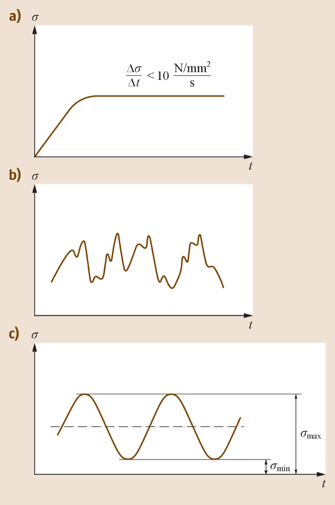

  

  Stress–time curves: (a) static, (b) dynamic (general arbitrarily oscillating), and (c) dynamic (idealized, uniformly oscillating)

• Dynamic stresses are (arbitrarily) changeable over time (Fig. 15.4a-cb). Periodic oscillation is a frequently occurring special case (Fig. 15.4a-cc).

In practice, the real change over time of an arbitrary dynamic load can frequently be idealized by a simply applied mathematical function (e. g., sine function) (Fig. 15.4a-cc).

The characteristics of a cycle are used to describe stress–time profiles (Fig. 15.5).

Fig. 15.5

Characteristics of a stress cycle

Distinctive characteristics are:

• The mean stress σ_m

• The stress amplitude σ_a

• The upper stress σ_up (= maximum stress σ_max)

• The lower stress σ_lo (= minimum stress σ_min)

• The (limit) stress ratio κ = σ_lo ∕ σ_up

The position of the mean stress σ_m relative to the zero stress line (σ = 0) is also important for the loading, or rather stress, of a component (Table 15.3). A differentiation is made between:

• The static stress (as a special case of stress in general)

• The repeated stress (cyclic stress, pulsating stress), which only change in the positive (compression) or in the negative (tension) area

• The alternating stress (alternating cyclic stress, reversing stress), in which the stress profiles intersect the zero line (constant change between tensile and compressive stress)

If different types of load act on a component simultaneously, the load cases can differ. For rough calculations, the correction factor α₀ can be used to convert the shear stress to the respective direct stress load case and can then be used in the modified equation for the equivalent stresses ((15.4)–(15.6)). Rough values for the correction factor are given in Table 15.4.

$$\begin{aligned} & \begin{aligned}\displaystyle&\displaystyle{\text{Maximum principal stress criterion:}}\\ \displaystyle&\displaystyle\sigma_{\mathrm{V}}=0.5\left[\sigma_{\mathrm{b}}+\sqrt{\sigma_{\mathrm{b}}^{2}+4\left(\alpha_{0}\tau_{\mathrm{t}}\right)^{2}}\right]\end{aligned}\end{aligned}$$

(15.4)

$$\begin{aligned} & \begin{aligned}\displaystyle&\displaystyle{\text{Maximum shear stress criterion:}}\\ \displaystyle&\displaystyle\sigma_{\mathrm{V}}=\sqrt{\sigma_{\mathrm{b}}^{2}+4\left(\alpha_{0}\tau_{\mathrm{t}}\right)^{2}}\end{aligned}\end{aligned}$$

(15.5)

$$\begin{aligned} & \begin{aligned}\displaystyle&\displaystyle{\text{Maximum shear strain energy criterion:}}\\ \displaystyle&\displaystyle\sigma_{\mathrm{V}}=\sqrt{\sigma_{\mathrm{b}}^{2}+3\left(\alpha_{0}\tau_{\mathrm{t}}\right)^{2}}\end{aligned}\end{aligned}$$

(15.6)

Load peaks can occur while dynamically loaded components are in service that exceed the nominal force (nominal load) or the nominal torque (rated torque) significantly. As these are very difficult to record by measurement in practice, they are taken into account in calculations by the application and service factor K_A (15.7). Values for the application and service factor can be found in Table 15.5.

$$\displaystyle F=K_{\mathrm{A}}F_{\mathrm{nom}}\quad{\text{and}}\quad T=K_{\mathrm{A}}T_{\mathrm{nom}}$$

(15.7)

Table 15.3 Stress cases and their representation

Table 15.4 Rough correction factors for steel (after Decker [15.3])

Table 15.5 Application and service factors K_A (based on ISO 6336-1 [15.4])

1.4 Strength Characteristics

In principle, a distinction is made between static and dynamic strength.

1.4.1 Static Strength

The static strength is generally determined by tensile testing and is represented in the stress–strain diagram (Fig. 15.6a,b).

Fig. 15.6a,b

Stress–strain diagram for steel (schematic) (a) with and (b) without a distinct yield point

Depending on the failure criterion, the dimensioning of the components is based on the elastic limit R_e or the ultimate strength R_m (fracture limit). Instead of R_e, the 0.2% proof strength R_p0.2 (yield strength) is used for brittle materials without a distinct yield point.

Depending on the loading mode (type of stress), the underlying material strengths result in the strength characteristics for steel materials at room temperature according to Table 15.6.

Table 15.6 Loading and corresponding static material characteristics for steel at room temperature (based on [15.2, 15.5])

1.4.2 Dynamic Strength

The stress fluctuations that occur due to dynamic loading can intensify at outer (geometric) and/or inner (metallurgical) notches and lead to damage to the material. Local exceeding of the ultimate strength can cause microcracks to form, which gradually grow into the component and ultimately lead to fatigue fracture.

A fatigue fracture is mostly characterized by smooth, bright fracture surfaces with arrest lines (also known as a clamshell pattern or beach marks) and a fast fracture (forced fracture) in the remaining cross section (fracture zone) (Fig. 15.7a-c).

Fig. 15.7a-c

Fast fracture (a), fatigue fracture under one-sided loading (b), and fatigue fracture under rotating bending load (c)

The sustainable load intensity depends on the number of load changes (cycles). If a test piece is loaded by a defined repeated load (alternating or cyclic) just under R_m, it can withstand N_D cycles before failure occurs. Different numbers of sustainable load cycles result depending on the level of the repeated load.

If the repeated load is sufficiently small, the test piece does not fail. The value of the load equals the fatigue strength and the corresponding number of cycles is the fatigue life N_FS. The fatigue strength of steel exists if the sustainable number of load cycles is N_FS > 10⁷. The graphic representation of the maximum possible repeated load above the corresponding number of cycles produces the so-called Wöhler curve (also known as a stress-cycle (S–N) curve) (Fig. 15.8).

Fig. 15.8

Wöhler curve for steel (schematic)

A component can be designed for a finite life or for infinite life. A component has a finite life if the stresses that occur exceed the value of the fatigue strength σ_FS (Fig. 15.9a,ba). If the stresses that occur are smaller than σ_FS, the component is considered to have an infinite life (Fig. 15.9a,bb).

Fig. 15.9a,b

Types of repeated stress and fatigue strength: (a) high cycle fatigue and (b) very high cycle fatigue

1.5 Strength-Reducing Effects

Strictly speaking, the strength characteristics described in the literature apply only to the standardized test piece with which they were determined. As the real components differ substantially from the test bars with regard to their size, shape, and surface properties, the material strengths determined by testing must be converted into the corresponding component strengths or component design strengths τ_G; σ_G. To do this, all strength-changing influencing factors (e. g., notch effect) must be taken into consideration.

1.5.1 Notch Effect

In a component without cross-sectional change, the force lines and nominal stresses are undisturbed. If the force line pattern or path is disturbed by cross-sectional changes (e. g., notches), force line compression (stress concentration) can occur in this area. This leads to nonuniform stress distribution with local stress peaks (Fig. 15.10a-ca,b), which reduces the load-bearing capacity of the component.

Fig. 15.10a-c

Stress distribution in notched components with the same stress cross sections: (a) force line profile in a tension bar, (b) stress distribution in the tension bar, and (c) influence of the notch shape on the stress peaks

The level of the stress peaks depends on the geometry of the discontinuity, also known as the stress raiser (notch). The more sharp-edged or acute-angled the notches are, the larger the stress peaks that occur at them (Fig. 15.10a-cc). The ratio of the stress peak σ_max and the calculated nominal stress σ_N = F ∕ A is called the theoretical stress concentration factor α_ki ≥ 1:

$$\displaystyle\alpha_{k\sigma}=\frac{\sigma_{\max}}{\sigma_{\mathrm{N}}}\quad{\text{and}}\quad\alpha_{k\tau}=\frac{\tau_{\max}}{\tau_{\mathrm{N}}}\;.$$

(15.8)

When the local stress peak σ_max is below the material yield point R_e, the value of the theoretical stress concentration factor α_ki of the notch depends only on the notch geometry and the loading mode. If the local stress peak lies above the material yield point, the effect of the notch increases with increasing material brittleness.

Ductile materials can partly minimize stress peaks that occur through locally limited yield. As a result, areas originally subjected to low stress become more highly loaded. The area immediately surrounding the notch is relieved, so that the notch effect is reduced compared to brittle materials with the same notch geometry. In this way, the areas further away from the notch have a support function for the near-notch areas.

The fatigue strength of a component is also changed by notches:

• The static strength (yield point) increases as a result of the support function from R_e to R_ek.

• The dynamic strength (alternating fatigue strength or amplitude fatigue strength) drops from σ_W and σ_A to σ_GW and σ_GA, respectively.

The ratio of the alternating fatigue strength of the smooth test bar σ_W and the alternating fatigue strength of the notched test bar σ_GW under the same conditions is defined as the fatigue notch factor β_k (for dynamic loading, by analogy for tangential stress):

$$\displaystyle\beta_{k}=\frac{\sigma_{\mathrm{W}}}{\sigma_{\mathrm{GW}}}=\frac{\sigma_{\mathrm{A}}}{\sigma_{\mathrm{GA}}}\;,$$

(15.9)

where 1 ≤ β_k ≤ α_k. For (brittle) materials completely sensitive to notches, β_k takes the value of the theoretical stress concentration factor of the notch α_k.

Values for the fatigue notch factor can be determined experimentally or can be taken from the appropriate literature (for example, [15.6, 15.7, 15.8]).

Relief notches can reduce the notch effect at design-related main notches through a more uniform stress profile (Fig. 15.11a-c).

Fig. 15.11a-c

Notch form and notch effect: (a) superimposition of notch planes, (b) relief notch in seized hub, and (c) relief notch on shaft shoulder

1.5.2 Other Influences

In addition to notches, the following factors also affect component strength:

• The surface roughness. Roughnesses act like small notches.

• The size effect. The higher strength of the boundary zone (e. g., through quenching and tempering) or geometrical size dependency of the stress gradients reduce the component strength with increasing component cross section, especially in bending and torsion.

• Surface hardening. Residual compressive stresses due to production-related surface hardening can increase the fatigue strength.

• The shape of the loaded cross section (rectangle, circle, etc.). This is taken into consideration in the stress concentration factor.

• The temperature. Higher temperatures reduce the strength, while lower temperatures increase the risk of brittle failure.

• The load frequency. Very high and very low frequencies reduce the alternating fatigue strength.

• The ambient medium. Aggressive media (e. g., saltwater) reduce the alternating fatigue strength.

• The support effect (i. e., higher strength values) is more favorable in terms of tension than in compression in gray cast iron.

The effect of the individual influences on the component strength is taken into consideration by corresponding influence factors, which are given in the relevant literature [15.10, 15.2, 15.3, 15.4, 15.5, 15.6, 15.7, 15.8, 15.9].

1.6 Practical Strength Calculation

The objective of component dimensioning is to specify the component dimensions, taking into consideration defined boundary conditions. These boundary conditions result from:

• Allowable stresses

• Allowable deformations

• Allowable heating

• Allowable speeds

• Allowable noise emissions

• Necessary life

This requires all influence factors acting on the component (e. g., forces, climatic conditions, and vibrations) to be known or identifiable.

Components that are mainly loaded mechanically are dimensioned on the basis of the allowable stresses, with consideration of the required safety factors. The strength values necessary for this are generally only available from static tensile tests. For rough estimate calculations, they can be used to approximately deduce the sustainable stresses for other static loads and stresses according to Table 15.7.

Table 15.7 Standard static strength characteristics for rough estimate calculations (approximate values, after [15.2])

The following relationship exists between the sustainable stresses and the allowable stresses:

$$\begin{gathered}\displaystyle\text{allowable stress}=\frac{\text{sustainable stress}}{\text{factor of safety}}\;.\end{gathered}$$

The durability of a component is considered to be assured, if

$$\begin{gathered}\displaystyle\text{sustainable stress}\leq\text{allowable stress}\;.\end{gathered}$$

For statically or mainly statically loaded components made of tough materials, the yield strength (yield point) R_e is decisive (or rather σ_bF or τ_tF) and for brittle materials the fracture strength R_m is decisive, from which

$$\displaystyle\sigma\leq\sigma_{\mathrm{all}}=\frac{R_{\mathrm{e}}}{S_{\mathrm{Y}}}\;,$$

(15.10)

or rather

$$\displaystyle\sigma\leq\sigma_{\mathrm{all}}=\frac{R_{\mathrm{m}}}{S_{\mathrm{F}}}\;,$$

(15.11)

where S_Y is the factor of safety against yielding in tough materials and S_F is the factor of safety against fracture in brittle materials.

For dynamically loaded components, for which the notch effect, size, and surface properties are initially unknown, the relevant fatigue strength is assumed initially

$$\displaystyle\sigma\leq\sigma_{\mathrm{all}}=\frac{\sigma_{\mathrm{D}}}{S_{\mathrm{D}}}\quad{\text{or}}\quad\tau\leq\tau_{\mathrm{all}}=\frac{\tau_{\mathrm{D}}}{S_{\mathrm{D}}}\;,$$

(15.12)

where S_D is a factor of safety against fatigue fracture. The allowable stresses (σ_all, τ_all) relate to the cross sections weakened by notches and/or grooves or the smaller cross sections in places with cross-sectional change.

The safety factors reduce the sustainable material strengths in calculation terms, as a result of which they allow for uncertainties and inaccuracies in the calculation operation (e. g., calculation with average values and simplifications in the calculation approach), the load assumption (e. g., load fluctuations that are difficult to record), and the material properties (e. g., scatter in the determination of strength values):

• The value of the safety factors to be used is essentially based on experience and is only partly defined in standards and guidelines.

The following aspects play a role when specifying the values:

• Smaller safety if the external loads can be reliably identified and recorded and failure does not have any disastrous consequences

• Larger safety if the external forces cannot be precisely identified or recorded and if failure can have disastrous consequences (e. g., risk to life and serious operational disruptions)

The effects must be carefully analyzed. A safety factor that is too high can also be fatal (apart from the economic viability or unviability). For example, in the case of components that heat up in service, it must be noted that the thermal stresses increase with increasing wall thickness and that the force effects induced by thermal expansion between fixed points become larger the stronger or sturdier the design. Table 15.8 gives an overview of standard, commonly used safety values.

Table 15.8 Standard safety values [15.2]

The (actual) available component safety can only be determined for components that have already been designed, as only then can all influences (size, notch effect, surface quality) be approximately recorded.

For a component subjected to static and dynamic loading, after it has been designed (dimensioning and form), the appropriate strength verifications (stress analyses) can be used to ensure that it satisfies the planned static and dynamic loading.

The general algorithm for performing strength verifications is illustrated graphically in Fig. 15.12.

Fig. 15.12

General algorithm for strength verification

1.6.1 Notes on Component Dimensioning and Design

The following steps must be worked through systematically when dimensioning and designing a component:

• Definition/determination of the external forces and moments (loads) acting on the component

• Rough calculation (and choice) of the dimensions based on allowable stresses, design, and functional requirements

• Design (including the details) of the component

• Calculation of the stresses occurring at the relevant parts of the component (stresses)

• Calculation of the static and dynamic component strengths (design strengths) for the relevant places on the component

• Determination of the existing safety and comparison with the required safety (static and dynamic strength verification (stress analysis))

If the existing safety is inadequate, the component must be modified (e. g., changing its dimensions, detailed design, and material as well as possibly its load and application points) so that the required safety is achieved. Repeated calculations are frequently necessary.

If an existing safety is disproportionately high, it is necessary to examine how improved utilization of the strength can be achieved. It may be possible to build smaller and more lightweight or to use more cost-effective materials with a lower strength. This frequently leads to solutions that are more favorable economically.

It should be noted that the required safety must be achieved at the critical places of the component, while for design reasons, other places can be overdimensioned with regard to strength (even with disproportionately high safety).

Other dimensioning criteria (deformation, heating, and wear) may also have to be considered in the assessment accordingly.

The specified allowable strength values must never be exceeded.

If use of a component requires compliance with several dimensioning criteria, all these criteria must be examined. The design must then be performed according to the failure criterion (failure limit) to be achieved first. Compliance with the remaining required criteria must be demonstrated.

1.7 Further Reading

Hibbeler [15.1], Young et al [15.11] and Issler et al [15.12] provide deeper insight into the mechanics of materials and the strength of materials.

Further information on service strength is provided by Lee et al [15.13], Haibach [15.14], Bannantine et al [15.15] and Manson and Halford [15.16]. In their book, Fatigue Assessment of Welded Joints by Local Approaches [15.17], Radaj et al discuss in particular the service strength of welded joints.

Guidelines for the calculated verification of component strength are given in the FKM Guidelines [15.5].

2 Fasteners

Fasteners (connecting elements) are used to joint components and/or to define their position relative to each other. They are used to transfer forces. The mode of action of the connection (joint) can be based on form closure (also known as positive locking), force closure (also known as force locking), or material bonding (Table 15.9).

Table 15.9 Modes of action of the fasteners and connectors

2.1 Modes of Action

In several jointing methods (e. g., riveted joints, keyed connections, and fitting bolts), several modes of action apply simultaneously so that clear separation between the modes of action is not possible.

2.2 Form-Closure Joints

2.2.1 General Information

Form-closure fasteners, such as bolts, pins, keys, woodruff keys, wedges, profiled shafts, and rivets, are all standardized and are available as standard components. They are characterized by the fact that, unlike force closure and material bonding, the components permanently or immovably connect together or continue to be able to move, e. g., the possibility for bolts to turn or sliding keys to be pushed. In addition, form-closure joints can normally be nondestructively undone, whereby the rivet constitutes an exception.

Form-closure fasteners are generally mainly subjected to surface pressure, shearing, and possibly bending and must be dimensioned according to these loading modes.

The calculation approaches listed in the following give an overview of the dimensioning of the individual fasteners. Here it must be noted that the calculation principles may need to be adapted to the specific calculation case.

2.2.2 Pinned Joints

Pinned joints are used:

• To form a fixed connection between wheel and lever hubs and axles or shafts

• To secure the position/centering machine parts

• As pins for fixing tabs, link plates, springs, etc.

• As overload protection (shear pins)

Application examples are shown in Fig. 15.13a-d.

Fig. 15.13a-d

Pinned joints (examples): (a) position fixing using parallel pins, (b) transverse pin jointing using tapered pin, (c) longitudinal pin with cylindrical grooved pin, and (d) cylindrical grooved pins (with neck) as pins

Depending on their shape, a differentiation is made between parallel pins, tapered pins, grooved pins, and spring-type straight pins (Fig. 15.14).

Fig. 15.14

Standardized pin types (selection) (after [15.18, 15.19, 15.20, 15.21, 15.22])

Parallel pins are primarily used for the fixed (tolerance grade m6) or loose (tolerance grade h8 or h11) connection of components. The holes in the components to be connected must be reamed to the required size limit according to the requirements, which results in high production costs.

Tapered pins are used in a similar way to parallel pins. Due to the tapered hole (expensive) the contact surfaces only briefly rub together on removing the pin, which results in low wear. Above all, they are suitable for precise positioning of components/devices that must be frequently undone or detached.

Grooved pins have several swaged grooves on their circumference with a raised portion on the side of each groove; these raised portions are deformed when knocked into the hole and produce a tight, interference fit on the hole. Due to the raised portions, tight hole tolerances are not necessary.

Axially slotted spring-type straight pins are an alternative to grooved pins. They are made of spring steel and have a large oversize (interference) of 0.2–0.5 mm. Due to their directional transverse load elasticity compared to parallel, tapered, and grooved pins, they tend to displace the pinned parts.

As a result of the applied forces and moments, pins are subjected to surface pressure and shear; shear pins are also subjected to bending (Fig. 15.15a-c).

Fig. 15.15a-c

Forces on pinned joints: (a) transverse pin, (b) push-fit pin, and (c) longitudinal pin

2.2.2.1 Transverse Pinned Joints

Transverse pin joints, which are for transferring a nominal torque T_nom, as in a lever hub (Fig. 15.15a-ca), must be checked for surface pressure and shearing in the case of larger forces.

With the symbols from Fig. 15.15a-c and the application and service factor K_A according to Table 15.5:

• The mean surface pressure p_N in the hub is

  $$\displaystyle p_{\mathrm{N}} =K_{\mathrm{A}}\frac{F_{\mathrm{nom}}}{ds} = K_{\mathrm{A}}\frac{T_{\mathrm{nom}}}{ds(d_{\mathrm{W}} + s)} \leq p_{\mathrm{all}}\;,$$

  (15.13)

  where:

  d :

  pin diameter

  D :

  external diameter of the hub

  d_W :

  shaft diameter

  s :

  pin width in the hub; $s={D-d_{\mathrm{w}}}/{2}$

• The maximum value of the mean surface pressure p_W in the shaft is

  $$\displaystyle\begin{aligned}\displaystyle p_{\mathrm{W}}&\displaystyle=4K_{\mathrm{A}}\frac{F_{\mathrm{W}\,\mathrm{nom}}}{dd_{\mathrm{w}}}=2K_{\mathrm{A}}\frac{3T_{\mathrm{nom}}}{2d_{\mathrm{W}}dd_{\mathrm{W}}/2}\\ \displaystyle&\displaystyle=K_{\mathrm{A}}\frac{6T_{\mathrm{nom}}}{dd_{\mathrm{W}}^{2}}\leq p_{\mathrm{all}}\;.\end{aligned}$$

  (15.14)

• For the mean shear stress τ_S in the pin

  $$\displaystyle\tau_{\mathrm{S}}=K_{\mathrm{A}}\frac{F_{\mathrm{W}\,\mathrm{nom}}}{A_{\mathrm{S}}}=K_{\mathrm{A}}\frac{4T_{\mathrm{nom}}}{d_{\mathrm{W}}\uppi d^{2}}\leq\tau_{\mathrm{s}\,\mathrm{all}}\;,$$

  (15.15)

  where:

  p_all :

  see Table 15.10 (multiply values by 0.7 for slotted straight pins)

  τ_s all :

  see Table 15.10 (multiply values by 0.8 for slotted straight pins)

From experience, for the design a pin diameter d = (0.2–0.3)d_W and hub wall thicknesses s = (0.25–0.5)d_W are chosen for steel hubs and s = 0.75d_W for gray cast iron hubs.

Table 15.10 Guide values for allowable stresses for bolted and pinned joints under approximately static load [15.23, 15.24]

2.2.2.2 Longitudinal Pinned Joints

Under the force F_N on the longitudinal pin (also round key) (Fig. 15.15a-cc), the mean surface pressure p is twice the magnitude of the shear stress τ_s.

Therefore, it is not necessary to calculate the shear stress in solid pins. The relevant mean surface pressure in both parts (shaft and hub) is calculated from

$$\displaystyle p=K_{\mathrm{A}}\frac{F_{\mathrm{nom}}}{A}=K_{\mathrm{A}}\frac{4T_{\mathrm{nom}}}{d_{\mathrm{W}}dl}\leq p_{\mathrm{all}}\;,$$

(15.16)

where Table 15.10 lists p_all values (multiply values by 0.7 for slotted straight pins.)

From experience, pin diameters d = (0.15–0.2)d_W and load-bearing pin lengths l = (1–1.5)d_W are chosen.

In the case of large torques, several pins can be arranged on the circumference.

2.2.2.3 Clevis Pin Joints

Clevis pins (Fig. 15.15a-cb) must be calculated for bending and for surface pressure. The transverse force (shear) can be ignored.

The bending stress σ_b must be verified with bending moment M_b = Fl:

$$\displaystyle\sigma_{\mathrm{b}}=K_{\mathrm{A}}\frac{M_{\mathrm{b}}}{W_{\mathrm{b}}}\approx K_{\mathrm{A}}\frac{M_{\mathrm{b}}}{0.1d^{3}}\leq\sigma_{\mathrm{b}\,\mathrm{all}}\;,$$

(15.17)

where:

σ_b all :

see Table 15.10 (multiply values by 0.7 for slotted straight pins)

W_b :

see Table 15.1

The surface pressure is made up of the component changeable along the hole $p_{1}=F(l+s/2)/(ds^{2}/6)$ (corresponds to p₁ = M_b ∕ W_b, where $M_{\mathrm{b}}=F(l+s/2)$ and W_b = d² ∕ 6 due to the bending stress profile as in a slab or plate) resulting from the overturning effect on the pin and the component constant along the hole p₂ = F ∕ (ds) resulting from the shearing effect of F.

The maximum mean surface pressure is then

$$\displaystyle\begin{aligned}\displaystyle p_{\max}&\displaystyle=p_{1}+p_{2}\\ \displaystyle&\displaystyle=K_{\mathrm{A}}\frac{F_{\mathrm{nom}}}{ds^{2}}\left(6l+4s\right)\leq p_{\mathrm{all}}\;,\end{aligned}$$

(15.18)

where Table 15.10 lists p_all values (multiply values by 0.7 for slotted straight pins).

2.2.3 Bolted Joints

Bolts are used to make preferably free-to-rotate joints (Fig. 15.16).

Fig. 15.16

Basic design and loading of a bolted joint with related dimensions

Taking into account their type of use, bolted joints are adapted according to the required fit tolerances and properties of the mating material. Thus, diameter tolerances h11 or h8 with appropriate choice of hole tolerance enable clearance or interference fit for different use cases. Movable bolted joints are subjected to wear at the contact points that slide on each other. This can be reduced by lubrication, suitable selection of the material combination or by using bearing bushes. The force transfer within the bolted joints loads the fasteners with bending, shear, and surface pressure, whereby in general for joints at rest, the bending load is decisive and for moving joints the surface pressure is decisive. Standard bolt forms for different applications are shown in Fig. 15.17a-d.

Fig. 15.17a-d

Bolt forms: (a) without head, (b) without head with split pin holes and washers, (c) with head, and (d) with head and split pin hole (after [15.25, 15.26])

Depending on the type of fit between the bolt and bar or between the bolt and fork, three different installation cases are possible, which lead to different types of bending moment profiles and thus to different stresses in the bolt. The possible installation cases and equations required for the calculation are shown in Table 15.11.

Table 15.11 Possible installation cases with the corresponding calculation equations

Guide values for the allowable stresses are shown in Table 15.10.

If sliding movement occurs in the bolted joint, this must be taken into account in the material selection. If necessary, the sliding surfaces must be lubricated and a significantly lower allowable surface pressure must be used.

In highly loaded hinged joints, in addition to the bolt and bar cross section, the strength of the cross sections at the bar head and the fork most at risk must also be checked.

2.2.4 Other Form-Closure Joints

2.2.4.1 Riveted Joints

Rivets are primarily used to join two or more overlapping components. Unlike welding procedures, dissimilar materials can be joined when cold, so that effects such as distortion, hardening, or (micro) structural changes are avoided. To make the classic rivet joint, a rivet is placed in an existing hole or hole to be made (exception: punch riveting with a semitubular rivet), fixed and is then plastically deformed from the opposite side, so that a rivet head forms (Fig. 15.18a-d). Here a differentiation is made between hot and cold riveting.

Fig. 15.18a-d

Classic riveting. (a) Position of the rivet and blankholder, (b) position of the clincher, (c) plastic forming of the head, (d) finished riveted joint

Hot riveting is primarily used for steel rivets with diameters of 10 mm and larger. The rivet, inserted when heated (approximately 1000^∘C), contracts due to cooling, resulting in the overlapping components being pressed together (force-closure joint).

With cold riveting, the radial widening of the rivet forms a primarily form-closure joint.

If the rear of the joint is not accessible, blind rivets (pop rivets) can be used (Fig. 15.19a-d). These are an economically favorable solution for many fastening tasks. Compared to conventional riveted joints, they can be made by one person.

Fig. 15.19a-d

Blind riveting process

With punch riveting, unlike the classic riveting process, making the hole before the actual riveting is omitted. With self-piercing riveting with solid rivets, the actual rivet simultaneously functions as a cutting punch and perforates the parts to be joined. The bottom sheet is then pressed by an appropriately shaped die into an all-round groove of the rivet (plastically deformed), which results in a form-closure joint (Fig. 15.20a,ba). With self-piercing riveting with semitubular rivets, the rivet also acts as a cutting punch; however, it does not completely penetrate the components to be jointed, and as a result a gas- and liquid-tight joint is formed (Fig. 15.20a,bb).

Fig. 15.20a,b

Punch (self-piercing) rivets: (a) solid rivet process and (b) semitubular rivet process (after [15.27])

Riveted joints are generally not nondestructively separable. They can only be undone by removing the rivet (or rather drilling out or cutting off the rivet head).

Other standard riveting processes are listed in Table 15.12.

Table 15.12 Riveting processes according to DIN 8593-5 [15.27]

The advantages and disadvantages of riveting methods are shown in Table 15.13.

Table 15.13 Advantages and disadvantages of rivet joints

Reference is made to the relevant literature for the calculation of riveted joints (design and strength verification), for example [15.2, 15.24].

2.2.4.2 Form-Closure Retaining Elements

Form-closure retaining elements, for example, retaining rings, cotter pins (split pins), setting rings, and axle holders (axle stays) are frequently used for axial fixing and locating (keeping in position) shafts and bearings.

Figure 15.21a-h shows different retaining rings for various application cases for installation in corresponding annular grooves in round bodies (e. g., axles, shafts, bolts, and pins) or in holes.

Fig. 15.21a-h

Types of retaining rings (selection). (a) Circlips for axles or shafts, (b) circlips for bores, (c) shim washer, (d) circlips for axles or shafts with enlarged locating surface, (e) circlips for bores with enlarged locating surface, (f) E-clips, (g) round wire snap ring, and (h) grip rings

When axial forces act on retaining rings they cause surface pressure on the load-bearing shoulders between the ring and groove, which must not exceed allowable values. In cases of doubt, these should be checked by calculation.

Axially mounted retaining rings according to DIN 471 [15.29] for metric round bodies (Fig. 15.21a-ha) and according to DIN 472 [15.30] for metric bores (Fig. 15.21a-hb) are most frequently used. Retaining rings for inch-measure round bodies and holes are also available. The dimensions for the retaining rings and corresponding groove are given in the manufacturers’ catalogs.

If the load-bearing surfaces are too small due to large chamfers or rounding on the annular grooves, or if axial clearances have to be levelled out, additional shim washers or supporting rings according to DIN 988 [15.31] are used in conjunction with the retaining rings according to DIN 471 and DIN 472 (Fig. 15.21a-hc).

The locating surfaces can also be enlarged using rings according to DIN 983 [15.32] and DIN 984 [15.33] (Fig. 15.21a-hd,e).

Radial mountable retaining washers according to DIN 6799 [15.34] (Fig. 15.21a-hf) (E-clips) are used for small shaft diameters. They surround the groove bottom, are radially resilient with segments, and form a relatively high shoulder.

Round wire snap rings according to DIN 9925 [15.35] and DIN 9926 [15.36] (Fig. 15.21a-hg) (external snap rings) for bores and shafts are used for axial position fixing for secondary purposes with small axial forces. They are often difficult to remove from holes.

Self-locking grip rings for shafts without a groove (Fig. 15.21a-hh) have a force-closure effect. They can be used to adjust axial clearances under small axial forces.

Snap rings for rolling bearings according to DIN 5417 [15.28] (Fig. 15.22a,b) can be used to fasten radial bearings with an annular groove according to DIN 616 [15.37].

Fig. 15.22a,b

Snap ring: (a) according to DIN 5417 and (b) installation example (after [15.28])

Laminar rings (Fig. 15.23) are an alternative to retaining rings according to DIN 471 and DIN 472. They can be mounted without special pliers and require less installation space due to their lack of eyes.

Fig. 15.23

Spiral rings for holes (left) and shafts (right)

The fact that in many cases, depending on the existing requirements, the use of retaining rings can achieve substantial design simplifications and thus save costs, is shown by the rolling bearing design in Fig. 15.24. Figure 15.24b requires fewer parts, less production work (smooth continuous housing hole, no thread), and is also more compact.

Fig. 15.24

Installation options for a rolling bearing as fixed bearing

Split pins (Fig. 15.25a,ba) are mainly used for loose, articulated pin joints and for bolted joints (castellated nuts). In general, they may only be used once and cannot be used for force transfer.

Fig. 15.25a,b

Split pins according to ISO 1234 [15.38] (a) and spring cotters according to DIN 11024 [15.39] (b) in their mounted condition

Spring cotters are used for bolted joints, which have to be undone often. Spring cotters are frequently captively connected to the assembly to be secured, for example, by a chain (Fig. 15.25a,bb).

2.3 Force-Closure Joints

Force-closure joints transfer forces from one component to another by friction between the components.

2.3.1 Modes of Action

The contact forces necessary in a force-closure joint can be generated by special clamping elements (e. g., screws, wedges, and clamping collars) or as contact forces, which arise between the components due to jointing with interference fit.

If additional clamping elements are used, the contact forces are produced by tensioning these elements with the components to be joined.

2.3.2 Threaded Fasteners

Screws and bolts are the elements used most to connect components. They are all standardized and can be nondestructively undone and reused.

Apart from fastening and connecting, screws and bolts are also used to set and adjust, to measure, to tension, and as leadscrews for translating rotational movements into longitudinal movements.

The advantages of bolted assemblies are shown in Table 15.14.

Table 15.14 Advantages and disadvantages of screwed joints

2.3.2.1 Mode of Action, Variants, and Descriptive Sizes

The screw or bolt thread can be thought of as being a cylinder with a helix-shaped notch. The notch usually runs rising clockwise (Fig. 15.26). The mating thread (nut or threaded hole) corresponds to the negative image of the screw or bolt thread.

Fig. 15.26

Creation of the screw line

The thread pitch P is the relative axial displacement between the screw (external thread) and nut (internal thread) in one screw turn. The pitch angle φ follows from the thread pitch P and the (mean) pitch diameter d₂ and is calculated as

$$\displaystyle\tan\phi=\frac{P}{\uppi d_{2}}\;;\quad\phi=\arctan\frac{P}{\uppi d_{2}}\;.$$

(15.19)

Depending on the intended use and underlying standard, the dimensions vary in detail within the thread form, so that in general there is no exchangeability between the individual thread types. Table 15.15 shows standard international thread forms with their corresponding designation.

Table 15.15 Overview of the most common types of thread

Coarse thread (for example metric ISO thread according to DIN 13-1 or UNC thread to ANSI B1.1) is used for fixing screws and bolts (and corresponding nuts) of all kinds.

The fine pitch thread (for example according to DIN 13-2, DIN 13-11, or UNF according to ANSI B1.1) is used for large dimensions, loads, and stresses, in thin-walled parts and for micrometers and adjustment screws.

Trapezoidal thread (for example according to DIN 103 or ANSI B1.5) is preferably used as a translation or power transmission thread on spindles, for example, in machine tools, presses, valves, and vices.

Buttress threads (for example, according to DIN 513 or ANSI B1.9) have a higher load capability compared to the trapezoidal thread due to the larger rounded thread roots and due to the larger thread engagement depth and their radial jump-out effect in the nut thread remains lower than in other thread forms. Buttress threads are used as single or multistart translation or power transmission threads for high one-sided loads, for example, in jackscrews and pressing spindles.

Round threads (for example, according to DIN 405) display almost no notch effect, however have only a small thread engagement depth. Due to their large root and thread clearance they are suitable as translation or power transmission threads in severe soiling conditions, for example, as coupling rods in railway carriage couplings.

In addition to the above-mentioned thread forms or thread types, there are other variants for special applications, some of which are standardized.

The thread and screw/bolt dimensions required for the calculation of threaded fasteners (fixing screws and bolts) are shown for metric ISO thread (coarse thread) in Table 15.16 and for inch-measure UNC threads in Table 15.17. Reference is made to relevant books of tables and standards for other thread forms.

Table 15.16 Metric ISO thread (coarse thread) according to DIN 13-1 (selection). Dimensions as defined in Fig. 15.27

Fig. 15.27

Thread sizes

Table 15.17 Unified national coarse (UNC) thread to ANSI B1.1 (inch measure) (selection). Dimensions as defined in Fig. 15.27

2.3.2.2 Calculation of Bolted Joints

The calculation method presented in the following for fixing screws and bolts is mainly based on the VDI Guideline 2230 Systematic calculation of highly stressed bolted joints–Joints with one cylindrical bolt [15.40, 15.41].

Bolted joints are generally loaded by:

• Transverse forces F_Q at right angles to the bolt axis (Fig. 15.28) and/or

• By tensile forces (bolt loads or forces) F_S along the bolt axis,

whereby the joint must be designed so that bending moments and shear forces in the bolt or screw are avoided as much as possible and it is loaded under tension only.

Fig. 15.28

Diagram showing the relevant number of bolts n and the friction pairings i_R in transversely loaded bolted joints

This does not include preloaded fit bolts, which are calculated like bolts for shear and surface pressure (hole friction).

If transverse forces F_Q occur, the bolts must be preloaded so that the friction force F_R > F_Q necessary for the required force closure is generated, i. e.,

$$\displaystyle\begin{aligned}\displaystyle F_{\mathrm{R}}=F_{\mathrm{V}\min}\mu ni_{\mathrm{R}}&\displaystyle\geq F_{\mathrm{Q}}S_{\mathrm{H}}\quad{\text{or}}\\ \displaystyle F_{\mathrm{V}\min}&\displaystyle\geq\frac{F_{\mathrm{Q}}S_{\mathrm{H}}}{\mu ni_{\mathrm{R}}}\;,\end{aligned}$$

(15.20)

where:

F_Q :

transverse force on the bolted joint

F_Vmin :

minimum preload in the bolt

μ :

coefficient of friction in the interface (separating joint) between the components to be connected (e. g., μ = 0.1–0.15 for dry steel–steel pairings)

n :

relevant number of bolts in the joint (Fig. 15.28)

i_R :

number of effective friction couples (friction pairing) (Fig. 15.28)

S_H :

adhesion safety factor: S_H ≈ 1.3 under static and S_H ≈ 1.5 under dynamic loading

Due to the elasticity of the bolt and the clamped parts, the bolted joint behaves like springs connected in parallel (Fig. 15.29), where the bolt acts as a tensile spring and the clamped parts act as compression springs.

Fig. 15.29

Centrically clamped bolted joint and corresponding spring model according to VDI 2230 (after [15.40])

The elongation of the bolt f_S is more or less proportional to the acting force F_S and can be calculated using (15.21):

$$\displaystyle f_{\mathrm{S}}=c_{\mathrm{S}}F_{\mathrm{S}}=\frac{1}{\delta_{\mathrm{S}}}F_{\mathrm{S}}\;,$$

(15.21)

where c_S is the spring stiffness of the bolt and δ_S is the resilience of the bolt.

The compression of the clamped parts f_P is calculated from

$$\displaystyle f_{\mathrm{P}}=c_{\mathrm{P}}F_{\mathrm{P}}=\frac{1}{\delta_{\mathrm{P}}}F_{\mathrm{P}}\;,$$

(15.22)

where c_P is the clamped length and δ_P is the modulus of elasticity of the clamped parts.

According to (15.23), the total resilience δ_S of the bolt is made up of the resiliences of the partial areas:

$$\displaystyle\delta_{\mathrm{S}}=\delta_{\mathrm{SK}}+\delta_{\mathrm{Gew}}+\delta_{\mathrm{GM}}+\sum_{1}^{n}\delta_{i}\;,$$

(15.23)

where:

δ_SK :

resilience of the bolt head

δ_Gew :

resilience of the exposed (protruding) thread

δ_GM :

resilience of the screwed-in thread

δ_i :

resilience of the cylindrical shank section i

The resilience of the bolt head of hexagon and hexagon socket head bolts can be calculated using

$$\displaystyle\delta_{\mathrm{SK}}=\frac{4l_{\mathrm{SK}}}{E_{\mathrm{S}}\uppi d}\;.$$

(15.24)

where:

l_SK :

height of the bolt head (Fig. 15.30); for hexagon head bolts l_SK = 0.5d and for hexagon socket head cap screws (bolts), l_SK = 0.4d

E_S :

modulus of elasticity of the bolt material

d :

nominal diameter of the thread (Fig. 15.30)

Fig. 15.30

Individual deformation areas of the bolt (after [15.40])

The resilience of the protruding thread, not screwed in, is calculated from

$$\displaystyle\delta_{\mathrm{Gew}}=\frac{4l_{\mathrm{Gew}}}{E_{\mathrm{S}}\uppi d_{3}}\;,$$

(15.25)

where:

l_Gew :

length of the protruding thread (Fig. 15.30)

d₃ :

core diameter of the thread (Fig. 15.30).

In the area of the screwed-in thread, the total resilience is made up of the resilience of the nut δ_M and of the thread δ_G as given by

$$\displaystyle\delta_{\mathrm{GM}}=\delta_{\mathrm{G}}+\delta_{\mathrm{M}}\;,$$

(15.26)

where

$$\displaystyle\delta_{\mathrm{G}}=\frac{4l_{\mathrm{G}}}{E_{\mathrm{S}}\uppi d_{3}}\;,$$

(15.27)

and

$$\displaystyle\delta_{\mathrm{M}}=\frac{4l_{\mathrm{M}}}{E_{\mathrm{M}}\uppi d}\;,$$

(15.28)

where:

l_G :

length of thread engagement; as a rule l_G = 0.5d

l_M :

height of the nut; for screw-in thread l_M = 0.33d and for through-bolted joints l_M = 0.4d

E_M :

modulus of elasticity of the nut

The resiliences of the individual shank areas can be calculated using (15.29):

$$\displaystyle\delta_{i}=\frac{4l_{i}}{E_{\mathrm{S}}\uppi d_{i}}\;,$$

(15.29)

where l_i is the shank length i and d_i is the shank diameter i.

Calculating the resilience of the clamped parts is significantly more difficult due to the more complex stress curve. Below the bolt head, a rotational paraboloid clamped body (solid) forms, at whose boundaries σ_y = 0 (Fig. 15.31). The spring stiffness or rather the resilience in this area is defined by:

$$\displaystyle\delta_{\mathrm{P}}=\int_{y=0}^{l_{\mathrm{K}}}\frac{\mathrm{d}y}{E\left(y\right)A\left(y\right)}\;.$$

(15.30)

In practical calculations, this deformation body is approximated by a deformation cone.

Fig. 15.31

Clamped body and derived deformation cone (after [15.40])

The complete distribution of an equivalent deformation cone in a cylindrical screw-in joint is shown in Fig. 15.32a-ca. If the deformation cone cannot form radially in full due to the limited component width, the cone is replaced by a sleeve in the relevant area (Fig. 15.32a-cb). In the special case in which the bolt head or nut bearing surface is larger than the external diameter of the clamped parts, only a deformation sleeve exists and not a deformation cone.

Fig. 15.32a-c

Completely formed equivalent deformation cone of a screw-in joint (a) and through-bolted joint with deformation cone and sleeve (b,c) according to VDI 2230 (after [15.40])

Complete formation of the deformation cone exists if

$$\displaystyle D_{\mathrm{A}}\geq D_{\mathrm{A},\mathrm{Gr}}=d_{\mathrm{W}}+wl_{\mathrm{K}}\tan\varphi\;,$$

(15.31)

where:

D_A :

external diameter of the clamped parts

D_A,Gr :

limiting diameter of the deformation cone

d_w :

bearing diameter of the bolt head; the nut

w :

joint coefficient:

w = 2 for screw-in joints

w = 1 for through-bolted joints

l_K :

clamped length (Fig. 15.32a-ca)

φ_K :

cone taper angle of the joint (15.32)

If (15.31) is not fulfilled, a deformation sleeve must be considered in addition to the deformation cone.

The angle of the deformation cone is calculated for screw-in joints as

$$\begin{gathered}\displaystyle\tan\varphi_{\mathrm{KE}}=0.348+0.013\ln\beta_{\mathrm{L}}+0.193\ln y\end{gathered}$$

and for through-bolted joints as

$$\displaystyle\tan\varphi_{\mathrm{KD}}=0.362+0.032\ln\left(\frac{\beta_{\mathrm{L}}}{2}\right)+0.153\ln y\;,$$

(15.32)

where: β_L = l_K ∕ d_w

$$\begin{gathered}\displaystyle y=\frac{D^{\prime}_{\mathrm{A}}}{d_{\mathrm{w}}}\end{gathered}$$

D ^′_A :

equivalent external diameter of the basic solid (Fig. 15.31)

The resilience of the individual deformation cone can be calculated using

$$\displaystyle\delta_{\mathrm{P}}^{\mathrm{V}}=\frac{\ln\left(\frac{\left(d_{\mathrm{w}}+d_{\mathrm{h}}\right)\left(d_{\mathrm{w}}+2l_{\mathrm{V}}\tan\varphi_{\mathrm{K}}-d_{\mathrm{h}}\right)}{\left(d_{\mathrm{w}}-d_{\mathrm{h}}\right)\left(d_{\mathrm{w}}+2l_{\mathrm{V}}\tan\varphi_{\mathrm{K}}+d_{\mathrm{h}}\right)}\right)}{E_{\mathrm{P}}d_{\mathrm{h}}\uppi\tan\varphi_{\mathrm{K}}}\;,$$

(15.33)

where d_h is hole diameter (Fig. 15.31) and the height of the deformation cone is

$$\displaystyle l_{\mathrm{V}}=\frac{D_{\mathrm{A}}-d_{\mathrm{w}}}{2\tan\varphi_{\mathrm{K}}}\leq\frac{wl_{\mathrm{K}}}{2}\;.$$

(15.34)

The resilience of the sleeve is calculated from

$$\displaystyle\delta_{\mathrm{P}}^{\mathrm{H}}=\frac{4l_{\mathrm{H}}}{E_{\mathrm{P}}\uppi\left(D_{\mathrm{A}}^{2}-d_{\mathrm{h}}^{2}\right)}\;,$$

(15.35)

where the height of the sleeve is

$$\displaystyle l_{\mathrm{H}}=l_{\mathrm{K}}-\frac{2l_{\mathrm{V}}}{w}\;.$$

(15.36)

From these equations, the total resilience is

$$\displaystyle\delta_{\mathrm{P}}=\frac{2}{w}\delta_{\mathrm{P}}^{\mathrm{V}}+\delta_{\mathrm{P}}^{\mathrm{H}}\;.$$

(15.37)

If several components with different moduli of elasticity are bolted together, the deformation bodies (cone and sleeve) must be broken down into corresponding partial areas j ; m with the same modulus of elasticity and the resilience calculated bit by bit.

In the area of the deformation cone, instead of the bolt head bearing diameter d_w, the end diameter of the adjacent cone d_w,i is used in (15.33), where

$$\displaystyle d_{\mathrm{w},i}=d_{\mathrm{w}}+2\tan\varphi\sum_{i=1}^{j}l_{i-1}\;.$$

(15.38)

Furthermore, in (15.33) and (15.35) the height of the deformation body, l_V or rather l_H, is replaced by the height l_i of the subsegment and the modulus of elasticity E_P is replaced by E_Pi.

The total resilience of the clamped parts is thus

$$\displaystyle\delta_{\mathrm{P}}=\sum_{i=1}^{j}\delta_{\mathrm{P}i}^{\mathrm{V}}+\sum_{i=j+1}^{m}\delta_{\mathrm{P}i}^{\mathrm{H}}\;.$$

(15.39)

Strictly speaking, the equations given only apply to cylindrical components with centrally inserted bolts. Rectangular flanges or multiple bolt joints are assumed to be approximately cylindrical, whereby the external diameter corresponds to twice the average edge distance in the interface.

For details of how to calculate eccentric bolted joints or multiple bolt joints, reference is made to the relevant literature, for example, VDI 2230-2 [15.41].

The resilience of the bolt and of the clamped parts can be used to construct the joint diagram of the joint. First the deformations of the parts are drawn on a diagram with the correct sign (+/−) (Fig. 15.33a,ba).

Fig. 15.33a,b

Deformation characteristics of the bolt and the clamped parts (a) and the resulting joint diagram (b)

The deformation characteristic of the clamped parts is then mirrored about the abscissa (x-axis) and is moved to the right in the first quadrant, until $|F_{\mathrm{PM}}|=|F_{\mathrm{SM}}|=|F_{\mathrm{M}}|$. The result is the joint diagram shown in Fig. 15.33a,bb with the assembly force F_M and the resulting deformation of the bolt f_SM, or rather the clamped parts f_PM.

The relatively small bearing surfaces in the threads, underneath the bolt head, or rather of the nut in conjunction with the surface roughness in the contact zones of the joint partners leads to high surface pressures in these areas, as a result of which creep and thus relaxation of the joint occurs. The amount of relaxation is called the embedding (set) f_Z and the resulting loss of force is called the loss of preload F_Z, where

$$\displaystyle F_{\mathrm{Z}}=\frac{f_{\mathrm{Z}}}{\left(\delta_{\mathrm{S}}+\delta_{\mathrm{P}}\right)}\;.$$

(15.40)

Guide values for the embedding are given in Table 15.18.

Table 15.18 Guide values for embedments of uncoated steel bolts and compact clamped parts made of steel depending on surface roughness [15.40]

As a result of the loss of preload, the assembly force F_Mmin of the bolt must be larger than the minimum preload required according to (15.20), so that

$$\displaystyle F_{\mathrm{M}\min}=F_{\mathrm{V}\min}+F_{\mathrm{Z}}\;.$$

(15.41)

The maximum assembly force F_Mmax allows for fluctuations in the assembly force due to imprecise tightening methods or errors in the determination of the coefficients of friction. It is obtained from

$$\displaystyle F_{\mathrm{M}\max}=\alpha_{\mathrm{A}}F_{\mathrm{M}\min}\;.$$

(15.42)

Values for the tightening factor α_A are given in Table 15.19.

Table 15.19 Guide values for tightening factor α_A

If a preloaded bolted joint is additionally loaded by an axial working load F_A directly underneath the bolt head, or rather the nut is tensioned, the bolt extends further by the amount f_SA, which causes the upsetting (compressive strain) of the clamped components to reduce by the same amount f_PA (Fig. 15.34).

Fig. 15.34

Joint diagram showing the main dimensional variables acting

The increase in axial bolt force due to the working load is called the additional bolt load F_SA:

$$\displaystyle F_{\mathrm{SA}}=\frac{\delta_{\mathrm{P}}}{\delta_{\mathrm{S}}+\delta_{\mathrm{P}}}F_{\mathrm{A}}=\Phi F_{\mathrm{A}}\;,$$

(15.43)

where the term Φ is the simplified dimensionless force ratio and

$$\displaystyle\Phi=\frac{\delta_{\mathrm{P}}}{\delta_{\mathrm{S}}+\delta_{\mathrm{P}}}\;.$$

(15.44)

While the bolt is subjected to additional loading due to the working load, the clamped parts are relieved by F_PA:

$$\displaystyle F_{\mathrm{PA}}=F_{\mathrm{A}}-F_{\mathrm{SA}}=\left(1-\Phi\right)F_{\mathrm{A}}\;.$$

(15.45)

As a result of the relieving of the clamped parts, the clamping force between them also reduces. The remaining residual clamp load is given by

$$\displaystyle F_{\mathrm{KR}}=F_{\mathrm{V}}-F_{\mathrm{PA}}=F_{\mathrm{V}}-\left(1-\Phi\right)F_{\mathrm{A}}\;.$$

(15.46)

The maximum bolt load (before embedding) is given by

$$\displaystyle\begin{aligned}\displaystyle F_{\mathrm{S}\max}&\displaystyle=\alpha_{\mathrm{A}}\left(F_{\mathrm{V}}+F_{\mathrm{Z}}\right)+F_{\mathrm{SA}}\\ \displaystyle&\displaystyle=F_{\mathrm{M}\max}+F_{\mathrm{SA}}\;.\end{aligned}$$

(15.47)

In practice, the working load does not generally act directly underneath the bolt head or rather the nut, as shown in Fig. 15.35a-ca. In most cases the load application point is in the area of the clamped parts, so that these are only partly relieved, while the compressive load increases in the remaining part (Fig. 15.35a-cb,c). As a result of the load application point shifted from the ideal point, the resilience of the bolt appears to be larger, while the resilience of the clamped parts is smaller.

Fig. 15.35a-c

Load introduction in the clamped parts: (a) simplified case, (b,c) general cases

The type of load introduction is taken into account in the calculation by the dimensionless load introduction factor n, such that

$$\displaystyle\Phi=n\Phi_{\mathrm{K}}\;,$$

(15.48)

where Φ_K is the simplified force ratio (15.44).

For the special case of load introduction directly underneath the bolt head, n = 1, so Φ = Φ_K. The force introduction factors for clamping cases deviating from this are given in Table 15.20, whereby the following points apply:

• The plates must have the same modulus of elasticity.

• The joint must be able to be classified as a joint type in Fig. 15.36 with regard to the position of the interface and load introduction point.

For rough bolt dimensioning of transversely loaded bolts, n = 1 can be assumed, as the resulting bolt load is highest in this case.

The assembly force required for the joint is generated by tightening the bolt with an appropriate tightening torque (wrench torque) M_A.

The tightening torque M_A is made up of

$$\displaystyle M_{\mathrm{A}}=M_{\mathrm{G}}M_{\mathrm{K}}\;,$$

(15.49)

where:

M_G :

friction moment (friction torque) in the screwed-in thread

M_K :

bearing friction moment (torque) in the contact area between the bolt head, or rather the nut, and the parts to be bolted

The friction torque in the thread is given by

$$\displaystyle M_{\mathrm{G}}=F_{\mathrm{M}\max}\frac{d_{2}}{2}\tan\left(\phi\pm\rho^{\prime}\right),$$

(15.50)

where:

d₂ :

pitch diameter of the thread

φ :

pitch angle (helix angle) of the thread (15.19)

ρ^′ :

friction angle of the thread

Table 15.20 Guide values for load introduction factor n depending on the joint type SV and the dimensions of the bolted joint according to VDI 2230 [15.40]. For an explanation, see Fig. 15.36

Fig. 15.36

Joint type and parameters for determining the load introduction factor according to VDI 2230 (after [15.40])

The plus sign in (15.50) applies to the tightening and the minus sign to the undoing of the bolt.

The friction angle of the thread is a notional variable and results from the coefficient of friction in the thread μ_G (Table 15.21) and the flank angle of the thread α.

$$\displaystyle\tan\rho^{\prime}=\mu^{\prime}_{\mathrm{G}}=\frac{\mu_{\mathrm{G}}}{\cos\left(\frac{\alpha}{2}\right)}$$

(15.51)

Threaded fasteners must be self-locking so that they do not undo themselves. The thread is self-locking if the pitch angle φ of the thread is smaller than the thread friction angle ρ^′, i. e., φ < ρ^′.

Table 15.21 Thread coefficients of friction μ_G after Schlecht [15.42]

For a metric ISO thread with flank angle 60^∘, μ ^′_G  ≈ 1.155μ_G. Thus (15.50) can be rearranged to

$$\displaystyle M_{\mathrm{G}}=F_{\mathrm{M}\max}\left(0.16P+0.58d_{2}\mu_{\mathrm{G}\min}\right),{ }$$

(15.52)

where P is the thread pitch (15.19) and μ_Gmin is the smallest coefficient of friction in the thread.

The bearing friction torque M_K is calculated from the assembly force F_Mmax on tightening the bolt:

$$\displaystyle M_{\mathrm{K}}=F_{\mathrm{M}\max}\frac{\left(d_{\mathrm{W}}+D_{\mathrm{Ki}}\right)}{4}=F_{\mathrm{M}\max}\frac{D_{\mathrm{Km}}}{2}\mu_{\mathrm{K}}\;,$$

(15.53)

where

d_W :

external diameter of the bolt head or nut bearing

(d_W ≈ 1.4d)

D_Ki :

internal diameter of the flat (planar) head bearing

D_Km :

mean bearing diameter at the nut or at the bolt head (D_Km ≈ 1.3d for metric hexagon head and head cap bolts and screws)

μ_K :

coefficient of friction (μ_K ≈ 0.12 for the normal case or similar to μ_G according to Table 15.21)

The thread torque M_G and the bearing friction torque M_K can be used to calculate the tightening torque (bolt torque):

$$\begin{aligned}M_{\mathrm{A}} & =M_{\mathrm{G}}+M_{\mathrm{K}}\end{aligned}$$

(15.54)

$$\begin{aligned} & =F_{\mathrm{M}\max}\left(\frac{d_{2}}{2}\right)\tan\left(\phi\pm\rho^{\prime}\right)+F_{\mathrm{M}\max}\,\mu_{\mathrm{K}}\frac{D_{\mathrm{Km}}}{2}\;,\end{aligned}$$

$$\begin{aligned}M_{\mathrm{A}} & =F_{\mathrm{M}\max}\left(0.16P+0.58d_{2}\,\mu_{\mathrm{G}\min}+\frac{D_{\mathrm{Km}}}{2}\mu_{\mathrm{K}}\right).\end{aligned}$$

(15.55)

Due to the scatter of the coefficients of friction (Table 15.21), when calculating tightening torques or when tightening screws and bolts, it should be borne in mind that with low coefficients of friction the same tightening torques can produce substantially larger preloads (bolt stresses) and with high coefficients of friction small preloads can result.

The assembly preload F_Mmax causes a tensile stress $\sigma_{\mathrm{M}}=F_{\mathrm{M}\max}/A_{0}$ in the loaded stress cross section (or shank cross section) A₀ = A_min.

As a result of the thread torque M_G according to (15.55), a torsional stress τ_t = M_G ∕ W_t, where $W_{\mathrm{t}}\approx\uppi d_{\min}^{3}/16$ is introduced into the bolt cross section.

According to the maximum shear strain energy hypothesis, this leads to an equivalent stress σ_V = σ_red:

$$\displaystyle\sigma_{\mathrm{v}}=\sigma_{\mathrm{red}}=\sqrt{\sigma_{\mathrm{M}}^{2}+3\tau_{\mathrm{t}}^{2}}\;.$$

(15.56)

In general, on tightening the bolted joint the maximum strength of the bolt is not utilized and this prevents exceeding the yield point in the service case. Usually, 90% of the yield point is used as the limit value, so that

$$\displaystyle\sigma_{\mathrm{red}}\leq 0.9R_{\mathrm{p}0.2}\;,$$

(15.57)

where R_p0.2 is the elasticity limit of the bolt material (Tables 15.24 and 15.25).

Furthermore, it must also be checked that the increase in bolt load as a result of the working load does not lead to plastic deformation:

$$\displaystyle F_{\mathrm{AS}}=n\Phi_{\mathrm{K}}F_{\mathrm{A}}\leq 0.1R_{\mathrm{p}0.2}A_{0}\;.$$

(15.58)

In addition to the allowable stresses in the bolt, the surface pressure on the bearing surfaces of the bolt head, or rather the nut, and the clamped parts must also be checked. In the assembled state this is done by calculating

$$\displaystyle p_{\mathrm{M}\max}=\frac{F_{\mathrm{M}\max}}{A_{\mathrm{p}\min}}\leq p_{\mathrm{G}}\;.$$

(15.59)

And in the service state

$$\displaystyle p_{\mathrm{B}\max}=\frac{\left(F_{\mathrm{V}\max}+F_{\mathrm{SA}\max}\right)}{A_{\mathrm{p}\min}}\leq p_{\mathrm{G}}\;,$$

(15.60)

where p_Mmax is the maximum surface pressure immediately after installation of the bolt, p_Bmax is the maximum surface pressure under service load, A_pmin is the minimum contact area, p_G is the allowable surface pressure on the boundary surfaces (interfaces) (VDI = limit surface pressure) (Table 15.22), F_Vmax is the maximum preload of the joint, and F_SAmax is the maximum additional bolt load.

Table 15.22 Allowable limit surface pressures (interface pressures) (after Wittel et al [15.2])

The nominal diameter of bolts and screws depending on the strength class is estimated according to Table 15.23, in conjunction with the Fig. 15.37.

Table 15.23 Preselection of screws and bolts according to VDI 2230-1 (after [15.40])

Fig. 15.37

Flow chart for rough screw/bolt selection according to VDI 2230-1 (after [15.40])

First, using the axial and/or transverse forces (loads) acting on the bolt F_A,Q, the next highest load is looked for in the first column of Table 15.23. Depending on the load case and assembly method, the choice must then be shifted a certain number of rows down. The sum of the rows to be moved down can be determined using the flow chart in Fig. 15.37. The necessary bolt diameter, depending on the bolt’s strength class, is found in the corresponding row, in columns 2–4.

Example 15.1

A bolted joint tightened with a torque wrench must withstand an eccentric, static axial load of 10000 N and an additional transverse force of 5000 N.

The screw has strength class 10.9.

Solution 15.1

According to Table 15.23, the next highest load is 10000 N (row 9).

$$\begin{gathered}\displaystyle\frac{F_{\mathrm{Q}\max}}{\mu}=\frac{{\mathrm{5000}}\,{\mathrm{N}}}{0.15}={\mathrm{3333.3}}\,{\mathrm{N}}<F_{\mathrm{A}}={\mathrm{10000}}\,{\mathrm{N}}\end{gathered}$$

From the flow chart, for this load case (static and eccentrically acting axial load), one row must be skipped.

In addition, due to the assembly using a torque wrench, the row selection must be moved downwards by an additional row.

Thus, the selection (row 9) must be moved downwards by an additional two rows, which gives row 11.

Thus, the necessary bolt diameter for the selected strength class (10.9) is 10 mm.

Bolts, screws, and nuts made of steel are classified in strength classes depending on the material strength. The strength classes for bolts and screws made of steel and alloyed steel with metric thread according to ISO 68-1 [15.44] are defined in EN ISO 898-1 [15.43] (Table 15.24).

Table 15.24 Strength classes, materials, and mechanical properties of screws, bolts, and studs according to EN ISO 898-1 (excerpt) [15.43]

The strength class of hexagon head screws and bolts and hexagon socket head cap screws and bolts is marked by two numbers separated by a dot on the top of the screw or bolt head. The first number indicates one hundredth of the minimum tensile strength R_m in N ∕ mm². The second number stands for 10 times the ratio R_e ∕ R_m, or rather R_p0.2 ∕ R_m.

Example 15.2

An example of the strength class

Strength class 5.6:

$$\begin{aligned}\displaystyle R_{\mathrm{m}}&\displaystyle=5\times 100={\mathrm{500}}\,{\mathrm{N/mm^{2}}}\\ \displaystyle R_{\mathrm{e};\mathrm{p0}.2}&\displaystyle=0.6R_{\mathrm{m}}=0.6\times 500\,\frac{{\mathrm{N}}}{{\mathrm{mm^{2}}}}=300\,\frac{{\mathrm{N}}}{{\mathrm{mm^{2}}}}\;.\end{aligned}$$

Several different specifications, some of which are similar, exist in parallel for imperial and inch-measure screws and bolts. The individual strength classes are marked on the screw or bolt head by a marking system, whereby the corresponding strength values are given in the relevant tables (Table 15.25).

Table 15.25 Strength classes for inch-measure screws and bolts according to SAE [15.45] and ASTM [15.46] (excerpt)

2.3.2.3 Design Guidelines for Bolted Joints

A small selection of examples of unfavorable and favorable designs of bolted joints is shown in Table 15.26.

Table 15.26 Design examples for bolted joints

2.3.2.4 Screw-/Bolt-Locking and Accessories

Dynamically loaded bolted joints must be locked to prevent them from loosening themselves. This can be done by using form closure, force closure or material-bonding screw or bolt locking.

Force-closure locking elements are spring-loaded components, whose spring load provides additional axial clamping force in the bolted joint and as a result increases the force closure (e. g., split washers, spring lock washers, and lock nuts) (Fig. 15.38a-ea–c). Force-closure bolt locking is also achieved by locking (clamping against each other) two nuts.

Fig. 15.38a-e

Locking elements: (a) bolt with split washer, (b) bolt with toothed lock washer, (c) nut with clamping part, (d) castellated nut with split pin, and (e) tab washer with long tab

Form-closure locking elements immobilize the nut or bolt head through their shape or deformation (Fig. 15.38a-ed,e).

Material-bonding locking is achieved by adhesive bonding of the bolt thread with the help of special adhesives (threadlockers) or by coating the bolt with special plastics in the factory.

These coloaded elements are partly standardized as accessory components for bolted joints.

If the material of the bolted parts is very soft, the pressure on the bearing surfaces of the components can be reduced by using (plain) washers.

2.4 Material-Bonded Joints

Material-bonded joints include, for example, adhesive bonding, welding and, soldering joining methods. What they have in common is that the parts to be joined (components) are permanently bonded together, either directly or by means of an additional substance. In general, undoing such joints involves damaging or destroying the components or rather the additional material.

2.4.1 Adhesive Bonding

In the case of adhesive bonding, components (mostly flat) are joined with the help of an adhesive, with the objective of transferring forces (loads) and/or achieving a sealing effect.

According to EN 923 [15.47], an adhesive is a “non-metallic substance capable of joining materials by surface bonding (adhesion), and the bond possessing adequate internal strength (cohesion).”

Adhesive bonding is one of the oldest jointing methods. Even in the Stone Age, people used natural adhesives such as tree gum or pitch to join together materials. The advantages (Table 15.27) of adhesive bonding, particularly the possibility of quickly and reliably bonding together different materials (composite construction), the easy automatability, and the development of special high-strength and aging-resistant adhesives mean that adhesive joints are still a modern jointing method and are used industrially to an ever-increasing extent.

Table 15.27 Advantages and disadvantages of adhesive joints

Fig. 15.39

Comparison of the stress distribution in riveting, welding, and adhesive bonding

Adhesive joints are now used on a large scale, among other things, to produce packaging in the consumer goods industry, in the wood-processing industry, and also to an increasing extent in vehicle manufacturing.

The adhesives used industrially nowadays are generally made of synthetically produced polymers. They can be divided into physically setting adhesives and chemically reacting adhesives, depending on their type of solidification mechanism.

Physically setting adhesives solidify by:

• Volatilization of solvent/dispersant (solvent-borne adhesive/dispersion adhesive)

• Melting and subsequent solidifying of the polymer (hot-melt adhesive)

• Gelling of a mixture of powdered thermoplastic polymers and liquid plasticizers through the addition of heat (plastisols)

Chemically reacting adhesives solidify due to a reaction of mostly one- or two-component systems at room temperature or at increased temperatures.

The technical properties and thus the possible uses of modern adhesives are vary widely. They are often especially adapted to the application case. A rough overview of industrially used adhesives is given in Table 15.28, whereby it should be noted that depending on the composition, the properties can vary within a wide framework. For this reason, refer to the corresponding data sheets of the manufacturers for precise information.

Table 15.28 Areas of application of standard adhesives (excerpt)

The strength of the adhesive joint decisively depends on the adhesive forces between the adhesive and the components to be joined. Although adhesives are now available that can be applied directly onto oily metal sheets, in general the surfaces must be cleaned and pretreated before joining. The adhesive forces can be increased, for example, by roughening or pickling the bond planes.

The wettability of plastic surfaces can be problematic due to their low surface energy. The wettability of plastics can be improved by treating them with reactive gases (for example ozone or fluorine), plasmas, or by flame treatment.

The special properties of adhesive bonds must be taken into consideration in their design. For example, adhesive bonds respond very sensitively to peel loading. Table 15.29 shows examples of appropriate, process-compatible designs of the adhesive joints.

Table 15.29 Design examples for adhesive joints

2.4.2 Welding

In welding, the parts to be joined and the optional filler material made of similar materials are melted. They form a joint melt and solidify together during subsequent cooling, as a result of which a permanent bond is formed. The welding process can be assisted by using welding auxiliaries (e. g., powder, pastes, or gases). The energy (heat) required for melting the materials can be provided directly by using gas flames, arcs, or radiation or indirectly by, for example, electrical current or friction heat.

Both metallic and nonmetallic materials (e. g., plastics and glass) can be bonded together.

2.4.3 Soldering

Soldering is a process characterized by the fact that a metallic filler material (solder) with a melting point significantly lower than that of the materials to be joined is used to join metallic components and the joint can form by adhesion and diffusion mechanisms.

Soldered joints can be undone under certain circumstances by melting the filler metal.

Apart from the different soldering methods, soldering is also divided into hard soldering and soft soldering.

In hard soldering (brazing) (at operating temperatures up to 1100^∘C) joints must be achieved that satisfy certain strength requirements.

In soft soldering (at operating temperatures below 450^∘C) the focus is on the sealing and/or electric conducting properties of the soldered joint. The strength requirements of the joint are secondary. It can be undone by melting the solder.

2.5 Further Reading

Further details on the calculation of fasteners and jointing compounds are given, for example, by Spotts et al [15.48], Wittel et al [15.2], Niemann et al [15.24] and Schlecht [15.42]. VDI guidelines 2230-1 [15.40] and 2230-2 [15.41] are the standard works for the calculation of fixing screws and bolts.

Information on individual welding procedures is given in Matthes and Schneider [15.49]. Details of the design of welded joints in structural steelwork are given in the Eurocode EN 1993-1-8 [15.50].

The adhesive bonding manual by Rasche [15.51] describes further literature on the topic.

3 Axles and Shafts

The primary task of axles and shafts is the storage of rotating machine elements such as rollers, wheels, or joints.

3.1 Standard Types

3.1.1 Axles

Axles are used to hold and support stationary, rotating, and swinging machine parts, for example, wheels or pulleys. By definition, they do not transfer torque. They are mainly loaded by transverse forces and bending moments. Longitudinal forces rarely occur.

A differentiation is made between fixed and rotating axles. In the case of fixed axles, mounted components rotate loosely on the fixed axle. Therefore, the loading and stresses are generally only caused at rest or repeated (cyclic, pulsating) by shear from the transverse forces and by bending. Rotating axles are defined by the fixed components, which turn with the bearing-mounted axle. The loading and stresses result from alternating and rotating bending. As a result of this, rotating axles with the same shape and material have less load-bearing capacity than a fixed axle.

3.1.2 Shafts

Shafts are rotating components used to transfer torque. The loads are caused by torsion, transverse forces, and bending moments. Additional longitudinal forces can occur in certain transmission elements, such as bevel gears or helical spur gears.

3.1.3 Journals

A journal is the name given to stepped axle and shaft ends, which are used for support and bearing. These elements can be cylindrical, conical, and spherical.

3.2 Special Types

3.2.1 Hollow Shafts and Axles

Axles and shafts with a through-hole are called hollow axles or hollow shafts, respectively.

The load-bearing capability of shafts under bending and torsion increases with the cube of the diameter. Due to the nonuniform distribution of the bending and torsion stress, the internal area of the shaft volume of a solid shaft is hardly used for the load-bearing capacity, however it increases the component weight noticeably. From this it follows that hollow shafts with the same load-bearing capacity have a lower weight than solid shafts. In this special type, if the strength remains constant, as the ratio d ∕ D increases the increase in the external diameter is far smaller than the reduction in weight (Fig. 15.40). For example, for the ratio d ∕ D = 0.6; the weight G of the hollow shaft is 30% less than the solid shaft. However, the diameter D increases by only approximately 5%. One disadvantage of the hollow shaft compared to the solid version is the amount of production work, cost, and disadvantageous stress distribution in force-closure shaft–hub connections.

Fig. 15.40

Comparison of solid shaft and hollow shaft

3.2.2 Other Special Types of Shafts

Flexible shafts are used to drive movable tools with fixed drives and low torques. Crankshafts are used to convert translational movement into rotational movement. Cardan shafts are used to transfer torques at nonaligned shaft ends. The different special types of shafts are shown in Fig. 15.41a-c.

Fig. 15.41a-c

Special types of shafts: (a) flexible shaft, (b) crankshaft, and (c) cardan shafts

3.3 Materials for Axles and Shafts

In addition to strength, the choice of material is influenced by other factors such as wear and corrosion resistance as well as high-temperature strength. Table 15.30 shows the standard materials used in practice for different application cases.

Table 15.30 Materials for axles and shafts (standard materials) [15.2, 15.52, 15.53]

3.4 Design Calculation

The main load on axles occurs as a result of bending. The rotational bending must be considered for rotating axles. Shear can be the priority loading of very short axles. In general, the main loading of shafts is caused by torsion (Fig. 15.42a-c).

Careful analysis of the loading conditions is generally indispensable, as the application of torsional moments and transverse forces can vary greatly.

Frequent causes of loading:

• Driving power (torque)

• Vibrations:

  • Inertia forces

  • Imbalances

• Preloading and circumferential forces of belts and chains (radial forces)

• Service factors:

  • Acceleration and braking

  • Drive and load characteristics

• Foundation vibrations

• Temperature effect

Fig. 15.42a-c

Different loading of axles and shafts. (a) Rope pulley with stationary axle (static bending), (b) rope pulley with rotating axle (rotating bending), and (c) belt pulley with drive shaft (torsion and bending)

A differentiation is made between two cases for the calculation of the given torque:

• a) If the installation space for the shaft is predefined by the overall design, the bearing spacing is known and thus the bending moment can be determined.

• b) If the installation space is unknown, the bearing spacing is determined by the shaft to be designed and the bending forces are initially unknown.

In case b) the diameter can thus only be determined temporarily in a rough calculation. The precise calculation is performed after the details have been defined (e. g., bearing spacing).

3.4.1 Determination of the Torques and Bending Moments

The nominal torque of a shaft to be transferred is formed as the quotient of the power to be transferred P and the angular velocity ω = 2πn:

$$\displaystyle T_{\mathrm{nom}}=\frac{P}{\omega}\;.$$

(15.61)

Equation (15.61) can be expressed as a numerical value equation with T_nom in Nm, P in kW, and n in min⁻¹ as follows:

$$\displaystyle T_{\mathrm{nom}}\approx 9550\frac{P}{n}\;.$$

(15.62)

The action forces (belt and tooth forces) must be determined based on the maximum torsional moment. The reaction forces (bearing forces) must be determined for all cases. The following simplifications are to be taken into consideration:

• External forces are applied as point loads.

• In the case of long hubs, the load is assumed to be uniformly distributed.

In Fig. 15.43 the forces and moment diagrams of a shaft with straight-cut spur gears are shown highly simplified (all forces lie within one plane and only tangential forces act on the teeth).

Fig. 15.43

Forces and moment diagrams of a shaft with straight-cut spur gears (simplified representation)

If the action forces do not lie within one plane they must be resolved vectorially. If additional axial forces act (e. g., on helical gears), as a result of the tilting effect, these produce an additional radial tilting moment with a corresponding radial bearing force, which must also be considered.

3.4.2 Determination of the Diameter

The allowable and actual loads and stresses are decisive for the dimensioning of the diameter of axles and shafts. However, under certain circumstances the deformations (twist angle or deflections) or the speeds (Sect. 15.3.5, Critical Speed) can be decisive for the definition of the diameter and require an adjustment. These aspects must be considered especially if higher requirements are set for the running accuracy and for longer shafts.

3.4.2.1 Determination of the Diameter from Bending (Axles)

The maximum bending stress in cylindrical axles is calculated from the maximum bending moment M_bmax and the section modulus W_b under pure bending (mostly assumed, as longitudinal forces generally have only a small influence):

$$\displaystyle\sigma_{\mathrm{b}\max}=\frac{M_{\mathrm{b}\max}}{W_{\mathrm{b}}}\leq\sigma_{\mathrm{b}\,\mathrm{all}}\;.$$

(15.63)

The minimum diameter d required for the cylindrical axle is calculated with the help of the axial section modulus W_b = πd³ ∕ 32 from

$$\displaystyle d\geq\sqrt[3]{\frac{32M_{\mathrm{b}}}{\uppi\sigma_{\mathrm{b}\,\mathrm{all}}}}\approx 2.17\sqrt[3]{\frac{M_{\mathrm{b}}}{\sigma_{\mathrm{b}\,\mathrm{all}}}}\;.$$

(15.64)

The allowable bending stress σ_b all is determined as a rough estimate depending on the type of loading and the existing influencing variables (e. g., notch effects). Indicative values for the allowable bending stress are shown in Table 15.31.

Table 15.31 Indicative values for allowable bending stress (after Niemann et al [15.24])

To save material and weight for heavy-duty axles and shafts that are mainly subjected to bending, in accordance with (15.65), they can also be executed as a beam with the same strength.

$$\displaystyle d\geq\sqrt[3]{\frac{32M_{\mathrm{b}x}}{\uppi\sigma_{\mathrm{b}\,\mathrm{all}}}}\approx 2.17\sqrt[3]{\frac{F_{\mathrm{A}}x}{\sigma_{\mathrm{b}\,\mathrm{all}}}}$$

(15.65)

If (15.65) is applied throughout, a body of revolution results, which is bound by a cubic parabola (Fig. 15.44).

Fig. 15.44

Beam with the same strength

The surface pressure in the bearing points must be handled in the same way as in a bolted joint (Sect. 15.2.2).

3.4.2.2 Determination of the Diameter from the Torsional Load (Shafts)

Pure torsional loading of shafts is rare, as additional bending is often present. The maximum torsional stress in solid cylindrical shafts is calculated from the torsional moment T and the polar section modulus W_p:

$$\displaystyle\tau_{\mathrm{t}\max}=\frac{T}{W_{\mathrm{p}}}\leq\tau_{\mathrm{t}\,\mathrm{all}}\;.$$

(15.66)

If W_p = πd³ ∕ 16, the requirement minimum diameter of the shaft is

$$\displaystyle d\geq\sqrt[3]{\frac{6T}{\uppi\tau_{\mathrm{t}\,\mathrm{all}}}}\approx 1.72\sqrt[3]{\frac{T}{\tau_{\mathrm{t}\,\mathrm{all}}}}\;.$$

(15.67)

The allowable torsional stress τ_t all is determined as an estimate value depending on the type of load and the influencing variables that exist (e. g., notch effects). Indicative values for the allowable torsional stress result after Niemann et al [15.24] from

$$\displaystyle\tau_{\mathrm{t}\,\mathrm{all}}=\frac{\sigma_{\mathrm{W}}}{\left({3}\ldots{}{6}\right)}.$$

(15.68)

When using (15.68), it must be taken into account that smaller safety values are used for light service and larger safety values for heavy-duty service.

3.4.2.3 Determination of the Diameter from Torsion and Bending

In practice, a combination of torsion and bending usually occurs in shafts, which produces a multiaxial stress state. An equivalent stress hypothesis can be used to transform the individual superimposed bending and torsional stresses into a single-axis stress state corresponding to pure tension or pure bending, which allows an equivalent stress to be calculated. In most cases, the equivalent stress for the calculation of shafts subjected to torsion and bending is formed on the basis of the Von Mises criterion (Sect. 15.1.2 or rather Sect. 15.1.3):

$$\displaystyle\sigma_{\mathrm{V}}=\sqrt{\sigma_{\mathrm{b}}^{2}+3\left(\alpha_{0}\tau_{\mathrm{t}}\right)^{2}}\leq\sigma_{\mathrm{all}}=\sigma_{\mathrm{b}\,\mathrm{all}}\;.$$

(15.69)

The equivalent moment M_V (equivalent bending moment with the same effect as the bending and torsional moment together) with σ_b = M_b ∕ W_b and $\tau_{\mathrm{t}}=T/\left(W_{\mathrm{p}}\right)=T/\left(2W_{\mathrm{b}}\right)$ is calculated from

$$\displaystyle M_{\mathrm{v}}=\sqrt{M_{\mathrm{b}}^{2}+0.75\left(\alpha_{0}T\right)^{2}}\;.$$

(15.70)

With the condition $\sigma_{\mathrm{V}}=M_{\mathrm{V}}/W_{\mathrm{b}}\leq\sigma_{\mathrm{b}\,\mathrm{all}}$, the required shaft diameter is

$$\displaystyle d\geq\sqrt[3]{\frac{32M_{\mathrm{v}}b^{\prime}}{\uppi\sigma_{\mathrm{b}\,\mathrm{all}}}}\approx 2.17\sqrt[3]{\frac{M_{\mathrm{v}}b^{\prime}}{\sigma_{\mathrm{b}\,\mathrm{all}}}}\;.$$

(15.71)

The factor b^′ for a solid or hollow shaft is:

$$\begin{aligned}{\text{Solid shaft:}} & \quad b^{\prime}=1\end{aligned}$$

(15.72)

$$\begin{aligned}{\text{Hollow shaft:}} & \quad b^{\prime}=\frac{1}{1-\left(d_{i}/d\right)^{4}}\end{aligned}$$

(15.73)

Depending on the type of load and the existing influencing variables (e. g., not effects), the allowable bending stress σ_b all is initially determined as an estimate value (Table 15.31).

For the initial design, the minimum shaft diameters determined above form the basic size and stand for the calculated required cross section. For the final definition, however, grooves, holes and other features must be considered. However, the executed core diameter d_c should not be less than the determined diameter d^′ (Fig. 15.45).

Fig. 15.45

Estimated and final shaft diameter

3.5 Check Calculations

Following the design of the axle or shaft, taking into account the determined minimum diameter, the strength of the component must be verified. In particular, this verification should be performed for areas in which cross-sectional weaknesses exist, such as thread undercuts, grooves, or shaft shoulders.

3.5.1 Strength Verification

The strength verification basically includes three calculation steps. In the first calculation step, the equivalent stress σ_V produced in the component by all applied forces and moments is calculated. The procedure for this is explained in Sect. 15.1.2. The fatigue strength σ_G of the component is determined in the second calculation step. This results from the material strength, taking into consideration all strength-reducing effects (Sects. 15.1.4 and 15.1.5). The strength verification is performed in the third step. It demonstrates that the safety S is greater or equal to the agreed safety S_agr

$$\displaystyle S=\frac{\sigma_{\mathrm{G}}}{\sigma_{\mathrm{V}}}\leq S_{\mathrm{agr}}\;.$$

(15.74)

The safety required depends on the application case and potential damage. For rough calculations, from practical experience: S_agr = 1.2…2.0.

A detailed strength verification procedure is described in the DIN 743 [15.9] standard and in the FKM guidelines [15.5].

3.5.2 Deformation Due to Bending Forces

For deformation due to bending forces, the deflection f of the axle or shaft and the inclination angle β of the elastic curve must be checked. These are decisively influenced by the acting forces and the elasticity of the material used. Increased deflection and inclination, especially in shafts with gears, leads to meshing faults on the teeth, which in turn results in noise generation and premature wear. In bearing positions, excessive inclination also results in increased bearing wear.

The deflection and inclination angle of the bending line can be determined both graphically using Mohr’s method and analytically via the elastic bending line or Castigliano’s theorem. In complex axle/shaft geometries or load conditions the deformation can be calculated with the help of numerical methods such as the finite element method.

Guide values for the allowable deflection are given in Table 15.32 and for the inclination angle in Table 15.33.

Table 15.32 Indicative values for allowable deflection (after Niemann et al [15.24])

Table 15.33 Indicative values for allowable inclination angle (after Niemann et al [15.24])

3.5.3 Deformation Due to Torsional Moments

For the dimensioning of longer shafts, for example, slewing gear shafts of slewing cranes or power take-off drive shafts in utility vehicles, the twist is decisive due to torques (Fig. 15.46). Together with torque fluctuations, these deformations can lead to vibrations. Furthermore, low torsional stiffness requires a large twist angle and consequently gives rise to a low critical speed.

Fig. 15.46

Elastic deformation under torsion

As a result of the described effects, the actual twist angle φ must be below the allowable twist angle φ_all (φ ≤ φ_all). Equation (15.75) can be used as indicative values for the allowable twist angle:

$$\displaystyle\varphi_{\mathrm{all}}=\left({0.25}\ldots{}{0.5}\right)\,\frac{{}^{\circ}}{\mathrm{m}}\,l\;.$$

(15.75)

3.5.4 Critical Speed

3.5.4.1 Vibration and Resonance

If a body is deformed elastically by a force F or rather by a torque T, it can be made to vibrate flexurally (bending) or torsionally (rotation) by the restoring force acting in the opposite direction after sudden withdrawal of the force (unloading).

With increasing stiffness (spring constant) and decreasing mass of the component, the vibration frequency increases. This is independent of the size of the exciting force, which only determines the vibrational amplitude. Consequently, all bodies have a certain constant natural frequency. Multibody systems with i = 1…n masses and i = 1…n springs, have n = 1…n natural frequencies.

If a body is made to vibrate by an excitation frequency that equals the natural frequency (or an integral multiple of it), the excitation frequency superimposes the natural frequency and resonance occurs. The vibration amplitude increases as a result, which can cause the axle or shaft to fracture.

Together with the coupled machine parts, rotating shafts and axles form vibratory systems. In general it must be considered that flexural and torsional vibrations are also caused by rotational frequencies induced as excitation and periodically varying forces and moments.

3.5.4.2 Critical Bending Speed

Due to nonrotationally symmetrical design elements (for example, parallel key connections) or production inaccuracies, the center of gravity of shafts and axles does not generally coincide with the center of rotation (Fig. 15.47).

Fig. 15.47

Deformation of the shaft by centrifugal force

If the shaft or axle rotates with angular velocity ω, the unbalance produces the centrifugal force F_C:

$$\displaystyle F_{\mathrm{C}}=mr\omega^{2}=m\left(f+e\right)\omega^{2}\;. $$

(15.76)

At the same time, a restoring force F_r dependent on the spring bending stiffness of c_b counteracts the centrifugal force:

$$\displaystyle F_{\mathrm{r}}=c_{\mathrm{b}}f\;.$$

(15.77)

In force equilibrium,

$$\displaystyle\begin{aligned}\displaystyle 0&\displaystyle={F_{\mathrm{r}}}-F_{\mathrm{C}}\\ \displaystyle&\displaystyle=m\left(f+e\right)\omega^{2}-c_{\mathrm{b}}f\;.\end{aligned}$$

(15.78)

Rearranging to obtain the deflection f we get

$$\displaystyle y=\frac{e}{\left(\frac{c_{\mathrm{b}}}{m\omega^{2}}-1\right)}\;.$$

(15.79)

From (15.79) it can be seen that in the case where ω² = c_b ∕ m, deflection tends to infinity, so that the critical angular velocity ω_C is

$$\displaystyle\omega_{\mathrm{C}}=\sqrt{\frac{c_{\mathrm{b}}}{m}}\;.$$

(15.80)

Accordingly, the critical bending speed is

$$\displaystyle n_{\mathrm{k}}=\frac{30}{\uppi}\sqrt{\frac{c_{\mathrm{b}}}{m}}\quad{\text{in }}\frac{1}{\min}\;.$$

(15.81)

Multisupport shafts with n masses also have n critical speeds, whereby in most cases the lowest critical speed is significant in practice. Due to the complexity of such a multimass system, the critical speed is mostly determined approximately using special calculation programs or is determined experimentally.

3.5.4.3 Torsional Critical Speed

A system of shafts with components fixed on it can also be characterized as a torsion rod. Torque impulses, for example, due to a pulsating drive torque in combustion engines, a critical torsional vibration can be caused with the natural frequency of the shaft system. Torsional vibration resonances occur, which can damage the shaft.

The torsional critical speed n_C of a single degree of freedom system () (e. g., torsion pendulum) is calculated from

$$\displaystyle n_{\mathrm{C}}=\frac{30}{\uppi}\sqrt{\frac{R_{\mathrm{t}}}{I_{m}}}\;,$$

(15.82)

where:

R_t :

torsion spring rate of the shaft in Nm

I_m :

moment of inertia in kg m²

For a shaft with two masses,

$$\displaystyle I_{m}=\frac{I_{m1}I_{m2}}{I_{m1}+I_{m2}}\;.$$

(15.83)

3.5.4.4 Conclusions for the Design of Shafts and Axles

Determining the deformation in multiple shouldered shafts and calculating the moments of inertia are difficult. For this reason, an exact calculated determination of the critical speeds with a reasonable calculation time is often only possible with very large effort. Furthermore, the influence of the environment and the shaft length on the system cannot be ignored. As a result of this, the natural frequency is often determined experimentally. For safe operation of the shaft, the excitation frequency (mostly the speed) should be at least 20% above or below the natural frequency.

When dimensioning, the following design measures must be considered to prevent resonance phenomena:

• The bearings must be positioned as closely as possible to the rotating discs. This achieves smaller deflection.

• Through careful balancing of shafts with rotating parts, smaller centrifugal forces occur.

• On the material side, the critical speeds can only be influenced by the modulus of elasticity or the shear modulus.

3.6 Further Reading

A deeper insight into the dimensioning of axles and shafts is given, among others, by Wittel et al [15.2] and the DIN 743 Part 1–4 series of standards [15.10, 15.7, 15.9].

In their book Maschinendynamik [15.54] (machine dynamics), Dresig and Holzweißig provide a standard reference on vibration analysis of machine parts.

4 Shaft–Hub Connections

Shaft–hub connections are standardized connections for fastening components, such as wheels, gears, pulleys, levers, etc., on shafts, axles, and journals. They are primarily used to transfer torques and rotary movements. In certain applications, however, bending moments (e. g., in the case of inclined shaft positions) or axial forces (e. g., in the case of helical gears) must also be transferred.

Depending on the type of force transfer, shaft–hub connections are divided into:

• Form-closure shaft–hub connections: The connection is made by a specific shape design (e. g., by spline profiles, serrations, or polygonal splines) or through additional elements (e. g., by parallel keys, Woodruff keys, or transverse pins/cross pins).

• Frictional shaft–hub connections: The connection is achieved by frictional clamping or pressing of the hub onto the shaft or axle (e. g., via interference fit assemblies/press fit, taper seats, or clamping elements).

• Preloaded form-closure shaft–hub connections: Combination of frictional and form-closure connections (primarily achieved through different types of wedges and compression connections secured by parallel keys).

• Material-bonding shaft–hub connections: The connection is made by material bonding (e. g., by adhesive bonding, soldering, or welding). In many cases the connection can only be undone by destroying it.

A selection aid for specifying a suitable shaft–hub connection is given in Table 15.34.

Table 15.34 Notes on the selection of shaft–hub connections (after Niemann et al [15.24])

4.1 Form-Closure Shaft–Hub Connections

Form-closure shaft–hub connections are simple and inexpensive in their structure and assembly. The form closure is achieved by appropriate shaping of the shaft and/or hub (e. g., serrated or polygonal connection) or by using additional components (e. g., parallel keys and pins). The torques to be transferred are resolved into tangential forces or surface pressure at the contact points of the parts to be joined. Axial forces can generally only be transferred in conjunction with additional axial fixing (for example, stops or shaft retaining rings).

4.1.1 Parallel Key Connection

Parallel key connections are the most frequently used form-closure shaft–hub connection for a torque acting on one side, for example, for belt pulleys, gears, and couplings.

They can be easily mounted, dismantled, and reused.

Frequently used forms according to DIN 6885-1 [15.55] (Fig. 15.48) are:

• Form A: high form with round end faces

• Form B: high form with straight end faces

Fig. 15.48

Parallel key connection. Mode of action and forms (selection) according to DIN 6885-1 [15.55]

For hubs that move longitudinally, for example, sliding gears in gear units, the parallel key with corresponding tolerances becomes a sliding key.

In conjunction with force fit (clamped seat) or taper seats, they are used as a so-called preloaded form-closure connection for position fixing.

The circumferential force F_u resulting from the torque is transferred via the side faces (flanks) of the parallel key. This results in loading of the side faces with surface pressure and shear in the interface between the shaft and hub. With standard parallel keys the surface pressure on the side faces is exceeded before the allowable shear stress is exceeded. For this reason, parallel keys must be dimensioned for surface pressure.

$$\begin{aligned} & \begin{aligned}\displaystyle&\displaystyle{\text{Surface pressure in the hub:}}\\ \displaystyle&\displaystyle p=\frac{F_{\mathrm{u}}}{\left(h-t_{1}\right)l_{\mathrm{t}}i\varphi}=\frac{2T}{d\left(h-t_{1}\right)l_{\mathrm{t}}i\varphi}\leq p_{\mathrm{all}}\end{aligned}\end{aligned}$$

(15.84)

$$\begin{aligned} & \begin{aligned}\displaystyle&\displaystyle{\text{Surface pressure in the shaft:}}\\ \displaystyle&\displaystyle p=\frac{F_{\mathrm{u}}}{t_{1}l_{\mathrm{t}}i\varphi}=\frac{2T}{dt_{1}l_{\mathrm{t}}i\varphi}\leq p_{\mathrm{all}}\end{aligned}\end{aligned}$$

(15.85)

where

F_u :

circumferential force F_u = 2T ∕ d

h :

parallel key height (Fig. 15.48)

t₁ :

shaft groove depth (Fig. 15.48)

l_t :

effective length of the parallel key

T :

torsional moment

d :

shaft diameter

i :

number of parallel keys

φ :

bearing factor φ = 1 if i = 1; φ = 0.75 if i > 1

p_all :

allowable pressures (Table 15.35)

For parallel keys with round end faces (feather keys) (Fig. 15.48), the load-bearing length (effective length) l_t is determined by deducing the width of the parallel key b from the total length l (l_t = l − b).

If more than one parallel key is used, the bearing factor φ allows for nonuniform load bearing of the individual parallel keys.

Dimensions and tolerances of the parallel keys for a given shaft diameter are given in the relevant standards/reference tables (DIN 6885-1 [15.55] for metric parallel keys and ANSI B17.1 [15.56] for inch-measure parallel keys).

Indicative values for allowable surface pressures p_all are given in Table 15.35. The dimensions of the hub depends on the joining diameter (Table 15.36).

Table 15.35 Allowable pressures for parallel keys made of steel in N ∕ mm²

Table 15.36 Empirical values for hub lengths l_N and hub external diameters d_N depending on the shaft diameter d

4.1.2 Woodruff Key Joint

Woodruff keys are frequently used in small machine tools and in vehicle construction to transfer smaller torques (Fig. 15.49). Compared to a normal parallel key connection, it is easier to produce and thus less expensive. However, at the same time, due to the deeper shaft groove, it leads to greater weakening of the shaft.

Fig. 15.49

Woodruff keys according to ISO 3912/ANSI B17.2

The dimensions of woodruff keys are defined in the ISO 3912 standard [15.57] and in the American code ANSI B17.2 [15.58].

The calculation is performed similarly to that for a parallel key connection, whereby in most cases the surface pressure in the hub groove is the limiting factor.

4.1.3 Profile Shaft Connections

Profile shaft connections transfer the torques (in the form of tangential forces) via several effective areas. They are suitable for higher, intermittent (shock-like) torques (including alternate torques). They have a very good centering effect, which results in low unbalance and uniform distribution of the circumferential load. They can also be designed as sliding hubs by choosing an appropriate fit.

Standard profile shaft connections are shown in Table 15.37.

Table 15.37 Standard profile shaft connections

4.1.4 Straight-Sided Spline Connections

The even number of male splines arranged on the circumference act like parallel keys. They are relatively inexpensive to produce and are used, for example, in gear units in combination with sliding hubs (gear wheel or clutch sleeve). A differentiation is made, depending on the type of centering effect, between:

• Internal centering: very precise centering; used in machine tools

• Flank centering: difficult to produce; advantageous for shock and alternate loading

4.1.5 Splined-Shaft Connections

Due to their large number of teeth, splined-shaft connections can absorb particularly large and intermittent (shock-like) forces. At the same time, the large number of teeth enables fine adjustment from tooth to tooth, as a result of which the angular position of actuating elements can be easily varied. The small tooth height leads to narrow hubs. Their cost-effective production and good adjustability makes them especially suitable for actuating elements. A differentiation is made between involute and serrated spline connections, depending on the shape of the teeth.

4.1.6 Polygonal Connections

These are used as separable connections in sliding or press-fit seats for the transfer of shock-like, intermittent torques. However, due to micromovements between the parts to be joined there is a risk of vibration fretting.

Tight or interference fit is possible, depending on the clearance chosen. Clearance fits are to be avoided due to the associated micromovements.

Triangular and rectangular profiles P3G and P4C (Table 15.37) are primarily used.

Compared to the P3G profile, the P4C profile is particularly suitable for connections that are intended to be longitudinally slidable under load (torque).

The profile geometries are usually turned on a profile lathe (shaft) or are broached using a broaching machine (hub).

4.1.7 Calculation of Profile Shaft Connections

Profile shaft connections are designed for surface pressure on the respective effective surfaces. For straight-sided spline and splined-shaft connections

$$\displaystyle p=\frac{2T}{d_{\mathrm{m}}hl_{\mathrm{t}}i\varphi}\leq p_{\mathrm{all}}\;,$$

(15.86)

where:

T :

torsional moment

d_m :

average profile diameter

h :

load-bearing tooth height

l_t :

effective length of the connection

i :

number of teeth

φ :

bearing factor:

splined shaft with internal centering::

φ  = 0.75

splined shaft with external centering::

φ  = 0.9

splined shaft with serrated toothing::

φ = 0.5

splined shaft with involute toothing::

φ = 0.75

p_all :

see Table 15.35

For P3G polygonal connections, the surface pressure must be checked using

$$\displaystyle p\approx\frac{T}{l_{\mathrm{t}}\left(0.75\uppi e_{1}d_{1}+0.05d_{1}^{2}\right)}\leq p_{\mathrm{all}}\;,$$

(15.87)

where e₁; d₁ is the geometrical profile size (Table 15.37).

For the P4C profile, the surface pressure is approximately

$$\displaystyle p\approx\frac{T}{l_{\mathrm{t}}\left(\uppi e_{\mathrm{r}}d_{\mathrm{r}}+0.05d_{\mathrm{r}}^{2}\right)}\leq p_{\mathrm{all}}\;,$$

(15.88)

where e_r; d_r is the geometrical profile size (Table 15.37)

The allowable surface pressures are given in Table 15.35.

4.2 Frictional Shaft–Hub Connection

Frictional connections generate the forces necessary for force and moment transfer solely through friction at the interfaces between the shaft and hub.

According to Coulomb’s friction law,

$$\displaystyle F_{\mu}=\mu_{\mathrm{i}}F_{\mathrm{n}}\;.$$

(15.89)

The friction coefficient μ_i used to calculate the friction forces is either the sliding coefficient of friction μ or the static coefficient of friction μ₀, depending of the form of friction present.

In frictional connections, the frictional force must always be larger than the forces to be transferred, so that for slip-free transfer of axial forces F_a and torques T = F_uD_F ∕ 2:

$$\begin{aligned} & \begin{aligned}\displaystyle&\displaystyle{\text{Axial force:}}\\ \displaystyle&\displaystyle F_{\mathrm{a}}\leq F_{\mu\mathrm{a}}=\frac{\mu_{0}F_{\mathrm{n}}}{S_{\mathrm{r}}}=\frac{\mu_{0}\uppi D_{\mathrm{F}}l_{\mathrm{F}}p_{\mathrm{F}}}{S_{\mathrm{r}}}\end{aligned}\end{aligned}$$

(15.90)

$$\begin{aligned} & \begin{aligned}\displaystyle&\displaystyle{\text{Torque:}}\\ \displaystyle&\displaystyle T\leq T_{\mu}=\mu_{0}F_{\mathrm{n}}\frac{D_{\mathrm{F}}}{2S_{\mathrm{r}}}=\frac{\mu_{0}\uppi D_{\mathrm{F}}^{2}l_{\mathrm{F}}p_{\mathrm{F}}}{2S_{\mathrm{r}}}\;,\end{aligned}\end{aligned}$$

(15.91)

where:

μ₀ :

static coefficient of friction (Table 15.38)

D_F :

nominal diameter of the joint

p_F :

surface pressure in the joint gap (joint compression, interference of the joint)

l_F :

specified factor of safety against plastic elongation (1–1.3)

S_r :

factor of safety against slipping (1.5–2)

The ability of a connection or joint to transfer forces and moments essentially depends on the coefficient of friction and the normal (perpendicular) force F_n.

While the coefficient of friction is highly dependent on the type of paired materials, the surface finish, the lubricated condition, and relative speed of the paired components (guide values in Tables 15.38 and 15.39), F_n is limited by the allowable surface pressure p_F all.

Table 15.38 Guide values for coefficients of friction of longitudinal press-fit connections with quick loading according to DIN 7190-1 [15.59]

Table 15.39 Coefficients of friction of transverse press-fit assemblies in longitudinal and circumferential direction on slipping according to DIN 7190-1 [15.59]

Frictional connections can basically be divided into (Fig. 15.50):

• Connections with and without intermediate parts

• Connections with cylindrical and tapered fit joints

Fig. 15.50

Classification of frictional shaft–hub connections

When selecting friction connections, in addition to the force closure, other properties such as self-centering, setting and adjustability, production and assembly costs, the necessary production tolerances, and the separability or reusability must also be considered.

Advantages and disadvantages of frictional shaft–hub connections are given in Table 15.40; execution examples are given in Fig. 15.51a-d.

Table 15.40 Advantages and disadvantages of frictional shaft–hub connections

Fig. 15.51a-d

Examples of frictional connections. (a) Cylindrical press-fit assembly, (b) conical press-fit assembly, (c) press-fit connection with intermediate parts (tapered clamping elements), and (d) compression connection

4.2.1 Cylindrical Compression (Press-Fit) Connections

The internal diameter of the external part D_Ai and the external diameter of the internal part D_Ia are chosen so that an oversize (interference) U results (Fig. 15.52). If the external part is joined with the internal part, the oversize causes surface pressure p_F, also called joint compression, in the joint gap. Combined with the existing coefficient of friction in the joint gap, a friction force results that enables the frictional transfer of axial or rather circumferential forces.

Fig. 15.52

Mode of action of a press-fit connection and force (load) distribution. Index i = internal; index a = external

Due to the elasticity of the clamped parts, they are permanently joined together, which makes correction of the hub position very difficult.

Cylindrical press-fit connections are mainly used for permanent connections, such as flywheels, belt pulleys, gears, plain bearing bushes in housings, and rolling bearing rings.

After the type of joining has been chosen, a differentiation is made between longitudinal press-fit connections, transverse press-fit connections, and press-fit connections to be mounted or dismantled with pressurized oil methods (Fig. 15.53a-d).

Fig. 15.53a-d

Press-fit connections. (a) Longitudinal press-fit connection, (b) transverse press-fit connection, (c) conical press-fit connection joined with pressurized oil method, and (d) cylindrical press-fit connection to be dismantled with pressurized oil method

Longitudinal press-fit connections are mostly joined at room temperature by pressing the shaft into the hub. A slight taper at the end of the shaft makes it easier to insert the shaft. The longitudinal displacement causes smoothing of the surface, as a result of which the adhesive force is less than in a transverse force joint. Lubricants reduce the sliding coefficient of friction and thus make it easier to press in the shaft. After joining, they are slowly displaced from the joint gap so that the full adhesive force is not reached until after a longer adhesion time (approximately 48 h).

In the case of transverse press-fit connections the oversize necessary for the force transfer is cancelled out by heating the hub and/or cooling the shaft, so that a clearance fit results. In this condition, the components can be joined without force. After the temperature has equalized, the press fit required for the force transfer results.

Similar to transverse press-fit connections, oil injection press-fit connections can be joined almost force-free. In this case, during assembly or dismantling, oil is injected from the outside under high pressure through a slightly tapered fitting joint, which causes the hub to widen slightly and a thin film of oil results between the shaft and hub, which separates the contact surfaces from each other. Thus, when the parts are pushed together only fluid friction acts. Cylindrically shaped press-fit connections cannot be joined by this method; however, it can be used to undo them. After joining, a waiting time of approximately 2 h is required before loading the joint. The advantages and disadvantages of cylindrical press-fit connections are listed in Table 15.41.

Table 15.41 Advantages and disadvantages of cylindrical press-fit connections

4.2.1.1 Practical Calculation of Cylindrical Press-Fit Connections

The press-fit connection is calculated based on the standard DIN 7190-1 [15.59], whereby the calculation sequence has been modified. In calculation terms, the smallest required oversize U_min and the largest allowable oversize U_max must be determined based on the minimum surface pressure required in the joint gap p_Fmin and the maximum allowable surface pressure in the joint gap p_Fall.

Calculation of the required and allowable oversizes requires knowledge of all other geometrical variables of the press-fit connection.

According to Table 15.42, the hub dimensions can be roughly defined depending on the joint diameter.

Table 15.42 Rough, estimated values for hub dimensions of press-fit connections

The stated calculation requires pure elastic deformation of the internal and external parts; in practice, certain proportions of plastic deformation are allowed. The DIN 7190-1 standard gives a simple calculation method for elastic-plastic loaded press-fit assemblies (interference fits) for limited application, which is not discussed any further here.

4.2.1.1.1 Smallest Required and Largest Allowable Joint Compression

For a given torsional moment T, or rather a given axial force F_a, (15.90) and (15.91) can be rearranged to determine the minimum joint compression p_Fmin necessary for safe and reliable transfer:

$$\begin{aligned} & \begin{aligned}\displaystyle&\displaystyle{\text{Pure torque:}}\\ \displaystyle&\displaystyle p_{\mathrm{F}\min}=\frac{2TS_{\mathrm{r}}}{\mu_{0}\uppi D_{\mathrm{F}}^{2}l_{\mathrm{F}}}\end{aligned}\end{aligned}$$

(15.92)

$$\begin{aligned} & \begin{aligned}\displaystyle&\displaystyle{\text{Pure axial force:}}\\ \displaystyle&\displaystyle p_{\mathrm{F}\min}=\frac{F_{\mathrm{a}}S_{\mathrm{r}}}{\mu_{0}\uppi D_{\mathrm{F}}l_{\mathrm{F}}}\end{aligned}\end{aligned}$$

(15.93)

$$\begin{aligned} & \begin{aligned}\displaystyle&\displaystyle{\text{Simultaneous axial force and torque:}}\hfil\\[1.5mm] \displaystyle&\displaystyle p_{\mathrm{F}\min}=\frac{\sqrt{{F_{\mathrm{a}}}^{2}+\left(\frac{2T}{D_{\mathrm{F}}}\right)^{2}}S_{\mathrm{r}}}{\mu_{0}\uppi D_{\mathrm{F}}l_{\mathrm{F}}}\end{aligned}\end{aligned}$$

(15.94)

The maximum allowable joint compression p_Fmax is limited by the allowable material strength in the hub, or rather in the shaft.

$$\begin{aligned} & \begin{aligned}\displaystyle&\displaystyle{\text{External part:}}\\ \displaystyle&\displaystyle p_{\mathrm{F}\max A}=\frac{1-Q_{\mathrm{A}}^{2}}{\sqrt{3}S_{\mathrm{PA}}}R_{\mathrm{el}\,A}\end{aligned}\end{aligned}$$

(15.95)

$$\begin{aligned} & \begin{aligned}\displaystyle&\displaystyle{\text{Internal part (hollow shaft):}}\\ \displaystyle&\displaystyle p_{\mathrm{F}\max\mathrm{I}}=\frac{1-Q_{\mathrm{i}}^{2}}{\sqrt{3}S_{\mathrm{PI}}}R_{\mathrm{el}\,\mathrm{I}}\end{aligned}\end{aligned}$$

(15.96)

$$\begin{aligned} & \begin{aligned}\displaystyle&\displaystyle{\text{Internal part (solid shaft):}}\\ \displaystyle&\displaystyle p_{\mathrm{F}\max\mathrm{I}}=\frac{2R_{\mathrm{el}\,\mathrm{I}}}{\sqrt{3}S_{\mathrm{PI}}}\end{aligned}\end{aligned}$$

(15.97)

where:

Q_A; Q_I:

diameter ratios Q_A = D_F ∕ D_Aa; Q_I = D_Ii ∕ D_F (Fig. 15.53a-da)

S_PA; S_PI:

specified factor of safety of the hub, or rather the shaft against plasticization (1–1.3)

R_el A; R_el I:

lower elasticity limit of the hub, or rather the shaft

For further calculation, the smallest value of the minimum allowable surface pressure according to (15.95)–(15.97) must be used.

4.2.1.1.2 Smallest Required and Largest Allowable Oversize

From the smallest required and largest allowable joint compression p_Fmin and p_Fmax, with joint diameter D_F and the auxiliary variable K according to (15.99), the smallest required and largest allowable adhesion Z_min and Z_max can be calculated as follows:

$$\displaystyle\begin{aligned}\displaystyle&\displaystyle{\text{Smallest required adhesion:}}\\ \displaystyle&\displaystyle Z_{\min}=\frac{p_{\mathrm{F}\min}D_{\mathrm{F}}}{E_{\mathrm{A}}}\hfil\\[1.5mm] \displaystyle&\displaystyle{\text{Largest allowable adhesion:}}\\ \displaystyle&\displaystyle Z_{\max}=\frac{p_{\mathrm{F}\max}D_{\mathrm{F}}}{E_{\mathrm{A}}}\end{aligned}$$

(15.98)

with

$$\displaystyle K=\frac{E_{\mathrm{A}}}{E_{\mathrm{I}}}\left(\frac{1+Q_{\mathrm{I}}^{2}}{1-Q_{\mathrm{I}}^{2}}-\upsilon_{\mathrm{I}}\right)+\frac{1+Q_{\mathrm{A}}^{2}}{1-Q_{\mathrm{A}}^{2}}+\upsilon_{\mathrm{A}}\;,$$

(15.99)

where:

E_A; E_I:

modulus of elasticity of the hub, or rather of the shaft, respectively

υ_A, υ_I:

Poisson’s ratio of the hub, or rather of the shaft, respectively

On joining the components, smoothing (plastic deformation) of the surface roughnesses causes a loss in oversize ΔU (Fig. 15.54). With smoothing amounts of the surfaces G_Ai ≈ 0.2R_zAi and G_Ia ≈ 0.2R_zIa, the total loss in oversize is:

$$\displaystyle\Updelta U=2G_{\mathrm{Ai}}+2G_{\mathrm{Ia}}=0.4\left(R_{\mathrm{zAi}}+R_{\mathrm{zIa}}\right).$$

(15.100)

The smallest required or largest allowable oversizes to be set in before joining are made up of the adhesions according to (15.98) and the loss of oversize according to (15.100) as follows:

$$\displaystyle\begin{aligned}\displaystyle&\displaystyle{\text{Smallest required oversize:}}&\displaystyle&\displaystyle U_{\min}=Z_{\min}+\Updelta U\\ \displaystyle&\displaystyle{\text{Largest allowable oversize:}}&\displaystyle&\displaystyle U_{\max}=Z_{\max}+\Updelta U\end{aligned}$$

(15.101)

The maximum allowable dimensional fluctuation of the components, the fit tolerance P_T, is defined by the oversizes U_min and U_max:

$$\displaystyle P_{\mathrm{T}}=U_{\max}-U_{\min}\;.$$

(15.102)

The fit tolerance P_T must be divided between the tolerance zones of the hole T_A and the shaft T_I:

$$\displaystyle P_{\mathrm{T}}=T_{\mathrm{A}}+T_{\mathrm{I}}\;.$$

(15.103)

Notes:

• In the case of very fast rotating press-fit connections, the centrifugal forces that occur can reduce the fitting joint pressure. For this reason, the effect of the speed on fast rotating connections must be checked (DIN 7190-1 [15.59]).

• If the press-fit assembly is loaded dynamically, the fatigue strength of the shaft must be verified using a suitable method (FKM guidelines [15.5] or DIN 743 [15.9]).

Fig. 15.54

Surface smoothing in the longitudinal joints of the components

4.2.1.1.3 Joining Temperatures for Transverse Press Fits

The clearance fit S_e required for unforced joining must be established by heating the hub and/or cooling the shaft. For the necessary clearance, depending on the joint diameter D_F or the maximum oversize U ^′_max measured at ambient temperature, the following conditions apply: $S_{\mathrm{e}}/D_{\mathrm{F}}\approx{\mathrm{10^{-3}}}$, or rather $S_{\mathrm{e}}/U_{\max}^{\prime}\approx 0.5$.

The joining temperature of the external part ϑ_A at known joining temperature of the internal part ϑ_I with ambient temperature ϑ, the coefficients of thermal expansion of the external and internal part α_A and α_I (Table 15.43) and the joint diameter D_F is approximately calculated as

$$\displaystyle\vartheta_{\mathrm{A}}\approx\vartheta+\frac{U_{\max}^{\prime}+S_{\mathrm{e}}}{\alpha_{\mathrm{A}}D_{\mathrm{F}}}+\frac{\alpha_{\mathrm{I}}}{\alpha_{\mathrm{A}}}\left(\vartheta_{\mathrm{I}}-\vartheta\right).$$

(15.104)

The maximum possible heating of the hub is limited by its temperature resistance. Above this temperature limit, material strength losses are to be expected due to structural changes in the material. Guide values for the maximum joining temperature are given in Table 15.44.

Table 15.43 Coefficients of thermal expansion according to DIN 7190-1 [15.59]

Table 15.44 Maximum joining temperatures [15.59]

4.2.1.1.4 Pressing-In and Pressing-Out Forces in Longitudinal Press-Fit Connections

The jointing force necessary to join the longitudinal press-fit connection is calculated from

$$\displaystyle F_{\mathrm{in}}=\uppi D_{\mathrm{F}}l_{\mathrm{F}}p^{\prime}_{\mathrm{F}\max}\mu\;,$$

(15.105)

where:

D_F :

joint diameter

l_F :

hub length

p ^′_Fmax :

largest joint compression ((15.106))

μ :

coefficient of friction on pressing in (Table 15.38)

The largest joint compression p ^′_Fmax present describes the joint compression that sets in under the stated largest oversize U ^′_max :

$$\displaystyle p^{\prime}_{\mathrm{F}\max}=\frac{\left(U_{\max}^{\prime}-\Updelta U\right)p_{\mathrm{F}\max}}{Z_{\max}}\;,$$

(15.106)

where:

U ^′_max :

available interference

ΔU :

interference loss (−100)

z_max :

largest allowable adhesion (15.98)

p_Fmax :

maximum allowable joint compression ((15.95)–(15.97))

Due to the static friction, a larger force is required for the pressing out, so that: F_out > F_in (Fig. 15.55). By inserting the static coefficient of friction μ₀ (Table 15.38) for μ in (15.105), the pressing-in force is specified on the safe side.

Fig. 15.55

Pressing-in and pressing-out forces in longitudinal press-fit connection

The empirical value $F_{\mathrm{in}}/D_{\mathrm{F}}=4{-}7\,{\mathrm{kN/mm}}$ is used for orientation.

4.3 Press-Fit Connection Through Hydrojoining

Unlike the classic longitudinal or rather transverse press-fit connection, with this type of connection a joint clearance exists between the hub and the hollow shaft before the joining. To produce the necessary joint compression for the force transfer, a pressure (joining pressure) is applied to the hollow shaft underneath the hub, which causes it to widen (Fig. 15.56a-c). The parts to be joined and the process parameters (joint gap, joining pressure) are matched with each other so that the shaft undergoes plastic deformation and the hub undergoes elastic deformation. As a result, even after the joining pressure is removed, a permanent surface pressure occurs between the parts to be joined, which enables frictional force transfer.

Fig. 15.56a-c

Production process for hydrojoining. (a) Clearance fit before joining, (b) maximum widening during the joining process, and (c) permanent widening after joining process

The advantages and disadvantages of hydrojoined press-fit connections are shown in Table 15.45.

Table 15.45 Advantages and disadvantages of hydrojoined press-fit connections

4.3.1 Conical Press-Fit Connections

In conical (tapered) press-fit connections the conical hub is pressed axially onto a (mainly attached to the end of the shaft) rotationally symmetrical cone (Fig. 15.51a-db). They are used to transfer dynamic forces and moments, for example, in wheel, disc and clutch hubs or in machine tools for holding the tools. Their advantages and disadvantages are clearly shown in Table 15.46.

Table 15.46 Advantages and disadvantages of conical press-fit connections

The internal and external part have the same cone taper angle or inclination angle α ∕ 2:

$$\displaystyle\tan\left(\frac{\alpha}{2}\right)=\frac{D_{1}-D_{2}}{2l}\;.$$

(15.107)

The cone inclination can also be given by the rate of taper:

$$\displaystyle C=\frac{D_{1}-D_{2}}{l}\;.$$

(15.108)

The following rates of taper are suggested in DIN 254 [15.60]:

Easily separable connection::

C = 1  :  5

Difficult to separate connection::

C = 1  :  10

Toolholders::

C = 1  :  20, C = 1  :  30, C = 1  :  50

Morse taper::

C = 1  :  19.002 to 1  :  20.047

Self-locking exists in the conical press-fit connection if the angle of friction ρ = arctan(μ₀) is larger than the taper angle α ∕ 2.

The conical press-fit connection can be calculated as described in the DIN 7190-2 [15.61] standard.

4.3.2 Clamping-Element Connections

In this type of connection, the load is transferred via an additional component, the clamping element. Clamping-element connections are a special type of conical connections. Axial clamping causes conical clamping elements to be elongated elastically in the tangential direction (external part) and compressed (internal part), which produces a surface pressure between the shaft surface and the clamping element, or rather between the clamping element and the hub hole. The advantages and disadvantages are shown in Table 15.47.

Table 15.47 Advantages and disadvantages of clamping-element connections

4.3.2.1 Tapered Clamping Elements

The mode of action of tapered clamping elements is similar to that of conical press-fit connections. They mostly consist of two rings pushed inside each other (clamping set), which are conical on their joint contact surface (Fig. 15.57a,b). The clamping set is cylindrical on the inside and outside, and is dimensioned so that it can be pushed into the hub or onto the shaft with clearance.

Fig. 15.57a,b

Tapered clamping elements, individually (a) and assembled (b)

If the two rings are pushed inside each other by an axial force (mostly generated by screws or bolts) (Fig. 15.57a,b), the external ring widens elastically, while the internal ring is compressed elastically. This radial deformation causes friction forces between the hub and clamping set and the shaft and clamping set, and these enable force transfer.

Several tapered clamping elements can be connected successively to transfer higher forces/torques. In this case, it must be noted that due to friction losses, the axial force acting on the individual elements reduces from element to element (Fig. 15.58).

Fig. 15.58

Force distribution of the contact forces in several successive tapered clamping elements

Refer to the manufacturers’ information for notes on dimensioning and calculation. The advantages and disadvantages of tapered clamping element are listed in Table 15.48.

Table 15.48 Advantages and disadvantages of tapered clamping elements

4.3.2.2 Ringfeder Clamping Sets

The mode of action of Ringfeder (brand name) clamping elements is the same as that of tapered clamping elements. They differ in that the elements for clamping (bolts) are already integrated in the clamping set (Fig. 15.59a,b).

Fig. 15.59a,b

Ringfeder clamping set (a) and assembled clamping set (b)

The advantages and disadvantages of Ringfeder clamping sets are described in Table 15.49.

Table 15.49 Advantages and disadvantages of Ringfeder clamping sets

In addition to Ringfeder clamping sets, other special clamping sets are available with the same mode of action. They differ in their number of conical friction surfaces and the way in which the contact force is produced (Fig. 15.60a-e).

Fig. 15.60a-e

Other clamping sets (selection): (a) self-centering internal clamping set (make: Klempex), (b) internal clamping set for transferring large torques (make: Stüwe), (c) clamp ring (make: Stüwe), (d) two-piece clamp ring (make: Stüwe), and (e) clamping set with hexagon nut

4.3.2.3 Taper Lock^® Connection

Taper Lock^® connections are an alternative to the fixing of standardized belt pulleys and sprockets with classic parallel key connection. In these connections, an external conical taper bush is pressed, with the help of studs, into a hub with a corresponding mating shape (Fig. 15.61). They have a parallel keyway for additional security against twisting. Due to its longitudinal slot, the taper bush has very high elasticity. The press-fit connection can be undone with the help of specially threaded dismantling holes.

Fig. 15.61

Connection with taper bush

The advantages and disadvantages of Taper Lock^® connections are shown in Table 15.50.

Table 15.50 Advantages and disadvantages of Taper Lock^® connections

4.3.3 Compression Connections

Compression connections are mainly used to fix belt pulleys and levers. The clamping forces necessary for the force transfer are applied by screws/bolts or tilting forces. Parallel keys or tangential keys are also frequently installed for position fixing in the case of larger loads.

Guide values for the selection of the hub dimensions depend on the shaft diameter d according to Table 15.51.

Table 15.51 Rough, estimated values for hub dimensions of compression connections

Depending on the direction of the clamping forces, the connections can be divided into axial and radial compression connections. In the case of axial compression connections, the hub or the flange is pressed onto the shaft by one or several bolts, which produces a force-closure connection (Fig. 15.62a-da,b). Radial compression connections can be achieved by hubs that are clamped with the help of bolts and that are slotted on one side or divided (Fig. 15.62a-dc,d).

Fig. 15.62a-d

Radial and axial compression connections. (a) Radially clamped with divided hub, (b) radially clamped with slotted hub, (c) axially clamped by circumferential bolts, and (d) axially clamped by central bolt

4.3.4 Keyed Joints

Keyed joints are preferably used for rough service and alternating, intermittent shock-like torques and low precision requirements, for example, for the fixed connection of heavy-duty discs, wheels, or clutches in large machines, excavators, cranes, agricultural machines, or heavy-duty machine tools.

Driving-in forces produce surface pressures and thus friction forces on the keys, which results in the superimposition of frictional and form-closure connections.

A differentiation is made between longitudinal key connections, which produce a frictional connection in normal service and cottered connections with a preloaded form-closure connection. The advantages and disadvantages of keyed connections are shown in Table 15.52.

Table 15.52 Advantages and disadvantages of keyed connections

4.3.4.1 Longitudinal Key Connections

In normal service, the force transfer is by means of force closure (clamping of the shaft and hub by means of longitudinally inserted key) (Fig. 15.63a-c). If the forces/moments to be transferred exceed the friction forces present, form-closure force transfer also occurs (except for hollow saddle key connections).

Fig. 15.63a-c

Longitudinal key connection with keyway (a), flat gib-head key (b), and hollow (saddle) key connection (c)

Longitudinal key connections are frequently used due to the ease with which they can be tightened and reclamped, and due to their reusability.

4.3.4.2 Cottered Joints

Cottered joints are used to connect parts that are mainly loaded in the longitudinal direction or as fixing and adjusting keys, for example, to secure tool tapers and as a clamping element in jig construction.

The disadvantages of this connection are the relatively high production costs, the unfavorable stress distribution, and the difficulty in controlling the driving-in force. A bolted connection can be a useful alternative.

The basic structure of a cottered connection is shown in Fig. 15.64.

Fig. 15.64

Cottered joints

To be on the safe side, keyed connections are frequently dimensioned in the same way as parallel key connections, as the size of the driving-in force and thus the friction force are often difficult to determine.

4.4 Further Reading

More information on shaft–hub connections is provided in the reference book of the same name by Kollmann [15.62].

5 Rolling Bearings

The main tasks of bearings are to guide components that move relative to each other as well as absorb and transfer the acting forces or loads. They should enable movements (rotation and translation) in the required degrees of freedom and inhibit them in unwanted degrees of freedom.

They can basically be divided into rolling bearings and plain bearings. The movement or force transfer in rolling bearings takes place via rolling elements, which are arranged between rings or discs. Rolling friction dominates, so energy losses are low. In the case of plain bearings (sometimes called sliding bearings), the surfaces moving relative to each other rub each other directly (Fig. 15.65a,b).

Rolling bearings, as maintenance-free or low-maintenance bearings, are preferably used under normal requirements, for example, in gear units, machine tools, conveyor systems, or all kinds of vehicles. They are also used in spindle guides and cradles/turrets, as they operate with low friction from a standstill and at low speeds and withstand large loads. Their advantages and disadvantages are given in Table 15.53.

Fig. 15.65a,b

Plain (a) and rolling (b) bearings

Table 15.53 Advantages and disadvantages of rolling bearings

5.1 Structure and Properties

5.1.1 Structure

A differentiation is made between radial rolling bearings (Fig. 15.66a-ca) and thrust rolling bearings (Fig. 15.66a-cb) depending on the type of position fixing.

Fig. 15.66a-c

Radial and thrust bearings (selection with installation examples). (a) Radial deep-groove ball bearings; (b) deep-groove thrust ball bearings, and (c) rolling element shapes

Depending on their type, radial rolling bearings can absorb axial forces in addition to radial forces, while rolling thrust bearings are generally only suitable for axial loads.

Rolling bearings are further subdivided depending on their rolling element geometry (Fig. 15.66a-cc) into:

• Ball bearings

• Cylindrical roller bearings

• Needle roller bearings

• Tapered roller bearings

• Barrel roller bearings

The basic structure of rolling bearings is shown in Fig. 15.67a,b:

• Radial bearings: outer ring, inner ring, rolling element, cage

• Thrust bearings: shaft washer, housing washer, rolling element, cage

Fig. 15.67a,b

Basic structure of a rolling bearing according to ISO 5593. (a) Radial bearing and (b) thrust bearing

The inner and outer ring, or rather shaft and housing washer, of the roller bearings, via corresponding tolerances, are in direct contact with the surroundings of the bearing position.

During service, with the help of the lubricant, an elastohydrodynamic lubricant film ( contact) builds up between the rolling elements and the raceways of the bearing rings or washers. A ring-shaped cage secures the position of the rolling elements (Fig. 15.67a,b).

5.1.2 Bearing Dimensions and Designation

The external dimensions for metric bearings (inside and outside diameter, width, height, chamfer dimensions) are internationally standardized in ISO 15 [15.63] (radial bearings), ISO 355 [15.64], DIN 720 [15.65] (tapered roller bearings), and ISO 104 [15.66] (thrust bearings). Rolling bearings with inch-size or imperial dimensions are available (for example, ANSI/ABMA 12.2 [15.67], ANSI/ABMA 19.2 [15.68]), but should no longer be used for new designs.

Bearing designation based on the DIN 623-1 [15.69] standard is widely used internationally. Here, the bearing designation is made up of a prefix, a basic designation, a suffix, and additional designations (characters or numbers).

5.1.2.1 Prefixes

Prefixes are used if applicable to identify certain individual rolling bearing parts or special bearing materials, for example:

K::

Cage with rolling elements

L::

Free ring of a separable bearing

R::

Bearing ring with roller and cage or needle roller and cage assembly

S::

Stainless steel

5.1.2.2 Basic Designation

The basic designation contains the bearing type in a coded form, the dimension series (width series for bearing width B and diameter series for the outer diameter D), and the bore diameter (bore ID number for the bore diameter d) (Fig. 15.68).

Fig. 15.68

Bearing designation according to DIN 623-1 (after [15.69])

5.1.2.3 Suffixes

Deviations from the standard version are to be given by suffixes.

As there are a large number of different suffixes, reference is made here to the bearing catalogs of the bearing manufacturers.

5.1.2.4 Additional Designation

Can contain additional information from the manufacturer.

5.2 Types, Properties, and Use

Table 15.54 gives an overview of the most commonly used types of rolling bearings.

Table 15.54 Overview of types of rolling bearings

Depending on the axial loadability and the installation situation, the following application cases result for radial bearings:

• As guide or fixed bearings (axial forces possible in both directions)

• As support bearings (axial forces possible in one direction)

• As a loose bearing (no absorption of axial forces)

Rolling bearings in which the external force is always divided into an axial and radial component, regardless of the load angle, are called angular contact bearings.

5.2.1 Standard Types

Many different types of rolling bearings are available. Table 15.55 gives a brief overview of the most commonly used types of rolling bearings.

Table 15.55 Overview of the most commonly used standard rolling bearings

5.2.1.1 Bearing Selection

For frequently occurring service cases and certain requirements, the bearing can be selected using Fig. 15.69. As deep-groove ball bearings are suitable for radial and for axial loads, have high running accuracy, have a small installation space, and are also readily available, their usability should be checked first.

Fig. 15.69

Selection of rolling bearings

5.3 Load Capacity and Life of the Rolling Bearings

5.3.1 Static Load Capacity According to ISO 76

In relation to rolling bearings, static loading is assumed if the bearing is loaded when it is at a standstill, at very low speeds (n < 10 min⁻¹), or during slow oscillatory movements. The forces acting on the bearing can be changeable over time (dynamic).

The static load capability is limited by the occurrence of plastic deformations in the contact point between the rolling elements and their raceway.

A rolling bearing is deemed to be statically operable if, at the contact point subject to the highest loading, the size of the total permanent deformation of the rolling element and raceway does not exceed 0.01% of the rolling element diameter.

The safety of a rolling bearing compared to the static loading is calculated from the ratio of the static load rating C₀ to the equivalent static load P₀ and is given in the form of the static safety factor S₀ as follows:

$$\displaystyle\begin{aligned}\displaystyle&\displaystyle{\text{For radial bearings:}}&\displaystyle&\displaystyle S_{0}=\frac{C_{0\mathrm{r}}}{P_{0\mathrm{r}}}\hfil\\[.5mm] \displaystyle&\displaystyle{\text{For thrust bearings:}}&\displaystyle&\displaystyle S_{0}=\frac{C_{0\mathrm{a}}}{P_{0\mathrm{a}}}\end{aligned}$$

(15.109)

Guide values for the static safety factor are given in Table 15.56.

Table 15.56 Guide values for the required static safety factor according to ISO 76 [15.70] (excerpt)

The static load rating C₀ of a rolling bearing equals the load at which a calculated stress of 4000–4600 MPa (depending on the bearing type) occurs at the contact points between the rolling elements and the raceways.

Values for C₀ are given in the corresponding catalogs of the relevant manufacturers or must be calculated with the help of the equations given in ISO 76 [15.70].

As the static load rating corresponds to pure radial loading for radial bearings and pure axial loading for thrust bearings, simultaneously occurring radial and axial forces F_r and F_a with radial and axial factors X₀ and Y₀ are to be summarized as an equivalent static load P₀.

The equation for the static equivalent radial load is

$$\displaystyle\begin{aligned}\displaystyle P_{0\mathrm{r}}&\displaystyle=X_{0}F_{\mathrm{r}}+Y_{0}F_{\mathrm{a}}\hfil\\[1mm] \displaystyle{\text{if }}F_{\mathrm{a}}&\displaystyle=0\quad{\text{then }}P_{0\mathrm{r}}=F_{\mathrm{r}}\;.\end{aligned}$$

(15.110)

Values for X₀ and Y₀ are given in Table 15.57 and the relevant information of the bearing manufacturers.

Table 15.57 Values for the factors X₀ and Y₀ according to ISO 76 (excerpt)

The static equivalent axial load can be calculated using

$$\displaystyle\begin{aligned}\displaystyle{\text{If }}\alpha\neq 90^{\circ}{\quad}{\text{then: }}P_{0\mathrm{a}}&\displaystyle=2.3F_{\mathrm{r}}\tan\alpha+F_{\mathrm{a}}\;;\hfil\\[1mm] \displaystyle{\text{if }}\alpha=90^{\circ}{\quad}{\text{then: }}P_{0\mathrm{a}}&\displaystyle=F_{\mathrm{a}}\;.\end{aligned}$$

(15.111)

Equation (15.111) applies to double-direction bearings for all ratios of radial to axial loads.

It applies to single-direction bearings under the following condition: F_r ∕ F_a ≤ 0.44cotα.

For spherical-roller thrust bearings simultaneously subjected to radial and axial loads:

$$\displaystyle P_{0}=F_{\mathrm{a}}+{2.5}\ldots{}{2.9}F_{\mathrm{r}}\;. $$

(15.112)

5.3.2 Dynamic Load Capability

During their service, rolling bearings are subject to wear, which limits their life. According to ISO 281, the life of a rolling bearing is defined as the number of revolutions completed by a bearing ring (or a bearing washer) in relation to the other bearing ring (other bearing washer), before the first indication of material fatigue becomes visible on one of the two rings (or washers) or on rolling elements [15.71].

Statements on the life of rolling bearings are of a statistical character, which means that the given/calculated values are subject to a certain scatter.

When calculating the life, a differentiation is made between the basic and the modified rating life.

5.3.2.1 Basic Rating Life

According to ISO 281, the basic rating life L₁₀ is the rating life associated with 90% reliability for bearings manufactured with commonly used high-quality material, of good manufacturing quality, and operating under conventional operating conditions [15.71]. From a statistical point of view, 10% of the bearings used can thus fail before reaching the basic rating life.

The basic rating of a bearing can be determined with the help of

$$\displaystyle\begin{aligned}\displaystyle&\displaystyle{\text{For radial bearings}}\\ \displaystyle&\displaystyle L_{10}=\left(\frac{C_{\mathrm{r}}}{P_{\mathrm{r}}}\right)^{p}{\mathrm{10^{6}}}{\text{ \textit{revolutions}}}\;;\hfil\\[1.5mm] \displaystyle&\displaystyle{\text{for thrust bearings}}\\ \displaystyle&\displaystyle L_{10}=\left(\frac{C_{\mathrm{a}}}{P_{\mathrm{r,a}}}\right)^{p}{\mathrm{10^{6}}}{\text{ \textit{revolutions}}}\;,\end{aligned}$$

(15.113)

where:

C_r,a :

dynamic load rating of the radial/thrust bearing

P_r,a :

equivalent bearing load of the radial/thrust bearing (15.114)

p :

life exponent for ball bearings: p = 3; for roller bearings p = 10 ∕ 3

The dynamic load rating C is the bearing load at which the bearing can statistically complete 10⁶ revolutions with a failure probability of 10%. It is given in the respective information of the rolling bearing manufacturers.

The life calculation using (15.113) applies to pure radial and axial loads. If radial and axial loads occur simultaneously, they must be converted into a dynamic equivalent load P_r;a, which has the same effect on the bearing as the pure radial or axial load such that,

$$\displaystyle P_{\mathrm{r;a}}=XF_{\mathrm{r}}+YF_{\mathrm{a}}\;,$$

(15.114)

where:

F_r :

actual radial load

F_a :

actual axial load

X :

radial factor

Y :

axial factor

The radial and axial factors for several selected bearing types are shown in Table 15.58.

Table 15.58 Values for radial factors X and axial factors Y for selected types of bearings according to ISO 281 [15.71] (excerpt)

Fig. 15.70

Axial factor Y and limit value for applicability e. Indicative values for f₀ (after Niemann et al [15.24]): deep-groove and angular ball bearings f₀ ≈ 14, roller bearings f₀ ≈ 35, and self-aligning and magneto ball bearings f₀ ≈ 2.5; for precise values, see ISO 76 (after [15.70])

For spherical roller thrust ball bearings simultaneously subjected to radial and axial load, under the condition F_r ≤ 0.55F_a,

$$\displaystyle P_{\mathrm{r;a}}=F_{\mathrm{a}}+1.2F_{\mathrm{r}}\;.$$

(15.115)

The life of a bearing is usually given in operating hours. With the given speed n in 1 ∕ min, (15.113) thus becomes

$$\displaystyle\begin{aligned}\displaystyle&\displaystyle{\text{for radial bearings:}}\\ \displaystyle&\displaystyle L_{{\mathrm{10}}\,{\mathrm{h}}}=\left(\frac{C_{\mathrm{r}}}{P_{\mathrm{r}}}\right)^{p}\frac{{\mathrm{10^{6}}}}{60n}{\quad}{\text{in h}}\;,\hfil\\[1.5mm] \displaystyle&\displaystyle{\text{and for thrust bearings:}}\\ \displaystyle&\displaystyle L_{{\mathrm{10}}\,{\mathrm{h}}}=\left(\frac{C_{\mathrm{a}}}{P_{\mathrm{a}}}\right)^{p}\frac{{\mathrm{10^{6}}}}{60n}{\quad}{\text{in h}}\;.\end{aligned}$$

(15.116)

A selection of guide values for the required basic rating lives in operating hours is given in Table 15.59.

Table 15.59 Guide values for the required basic rating lives L_10 h of ball bearings and roller bearings (selection) (according to Schaeffler [15.72])

5.3.2.2 Modified Life

The basic rating life calculated with the help of the equations above applies to normal material qualities under standard operating conditions.

The actual life of the rolling bearings, however, is highly influenced by other criteria:

• Lubrication of the bearing (type and viscosity of the lubricant, contained additives)

• Material properties (purity, hardness, fatigue limit, surface quality, temperature resistance)

• Internal stresses (due to production or assembly)

• Ambient conditions (dirt, moisture)

With the help of the modified rating life, compared to the basic rating life, more precise values can be determined for the durability of the bearings under the specific use conditions.

Detailed calculation steps are given in the ISO 281 standard [15.71] or the calculation regulations of the individual manufacturers.

5.3.3 Minimum Bearing Load

A minimum force (axial or radial, depending on the bearing type) is required to ensure correct rolling of the rolling elements on the contact surfaces.

As a rough guide value, the bearing load for ball bearings and for roller bearings should not fall below 1 and 2%, respectively, of the dynamic load capability.

When in doubt, follow the regulations of the individual bearing manufacturers.

5.4 Design

In addition to suitable bearing selection, the design of the bearings must also consider the bearing arrangement, the installation tolerances, and the lubricant supply with the corresponding seals.

5.4.1 Bearing Arrangements

Bearings must basically be arranged so that the components can be guided both axially and radially. Depending on the amount and direction of the actual loads, running accuracy requirements, and assembly and dismantling options, a suitable arrangement must be chosen for the rolling bearings. A differentiation is made between fixed-loose bearings, spring-loaded or preloaded bearings, and floating bearings (support bearings). The features and examples for the individual bearings are shown in Table 15.60.

Table 15.60 Features and examples of different bearings

5.4.2 Installation Guidelines

The design of the bearing seat on the shaft or in the housing essentially depends on the task (fixed or loose bearings) and the type of load (point or circumferential load).

The bearings must be fixed onto the shaft or in the housing in both the radial and in the axial direction (except loose bearings). The radial fixing is achieved via appropriately designed fits. Oversize fit is necessary if a circumferential load acts on the bearing ring (inner or outer ring). If the load direction relative to the bearing ring does not change (point load), a transition fit or slight clearance fit is allowed.

In the axial direction, the fixing is mostly achieved by one-sided ridge and steps/shoulders, whereby moving in the opposite direction is prevented by retaining rings, threaded fasteners, or the housing cover (Figs. 15.71a-c and 15.72a-d).

Fig. 15.71a-c

Axial fixing of rolling bearings in the housing: (a) through cover and rib, (b) through retaining rings, and (c) through bearing with groove and snap ring

Fig. 15.72a-d

Axial fixing of rolling bearings on the shaft: (a) with slotted nut, (b) with end washer, (c) with retaining ring, and (d) taper seat with slotted nut

5.5 Lubrication of the Rolling Bearings

The life of rolling bearings depends to a decisive degree on their lubrication. During the rolling operation, a thin film of lubricant should form between the parts moving relative to each other in the bearing (rolling element, raceways, and cage); this film separates the contact surfaces from each other and thus reduces wear significantly. In addition, the lubricant should protect the bearing against corrosion, remove any friction heat that occurs, dampen vibrations, remove abraded material (circulating oil lubrication), or bind abraded material (permanent lubrication). To a limited extent, bearings with a grease fill also have a sealing effect.

5.5.1 Selection of the Lubrication Method

Choice of the correct lubrication method and the corresponding lubricant should take place at the beginning of the bearing design. The choice of suitable lubrication method depends, among other things, on:

• The size and type of bearing

• The operating conditions

• The running quietness/smooth running requirements

• The connection design

Depending on the lubricant used, a differentiation is basically made between grease, oil, and solid lubrication, although solid lubrication is only seldom used.

The advantages and disadvantages of grease and oil lubrication are listed in Table 15.61.

Table 15.61 Advantages and disadvantages of grease and oil lubrication

In practice, approximately 90% of all rolling bearings are lubricated with grease. As the lubricants age due to thermal and mechanical loading and also become contaminated due to abraded material and dirt input, their life is limited. If replacement of the lubricant (relubrication) is not possible, as for example with two-sided sealed bearings, the service life of the lubricant can, under certain circumstances, constitute the limiting factor in the bearing life consideration.

5.6 Sealing of Rolling Bearings

The sealing of rolling bearings should essentially fulfill two functions:

• 1. Sealing the bearing against gaseous, liquid, and/or solid substances/contamination

• 2. Prevent the escape of lubricant

To achieve this, the bearings themselves can have a seal (for example RS bearings or Z bearings) or the surroundings of the bearing must be sealed accordingly. More detailed information on the possible sealing systems is given in Sect. 15.7.

5.7 Rolling Bearing Damage

If installed correctly and operated as intended, rolling bearings are very reliable and are generally largely maintenance free.

Statistically, only 0.335% of all rolling bearings fail prematurely as a result of production or material errors [15.73].

Premature failure of a bearing significantly before the rated life L_10 h, is generally viewed as being bearing damage.

The most frequent causes of bearing damage are shown graphically in Fig. 15.73.

Fig. 15.73

Causes of bearing damage (after [15.74, 15.75])

The bearing damage that occurs can be divided into six different categories according to ISO 15243 [15.76] (Fig. 15.74).

Fig. 15.74

Types of damage to rolling bearings according to ISO 15243 (after [15.76])

5.7.1 Bearing Damage Due to Fatigue

Fatigue is the term used to describe the flaking or spalling of surface layers as a result of cyclical loading of the contact surfaces.

Depending on the origin of the damage, a differentiation is also made between subsurface-initiated fatigue (fatigue beginning under the surface) and surface-initiated fatigue (fatigue beginning on the surface).

Subsurface-initiated fatigue in the form of microcracks under the surface is caused by continuous rolling over the contact surfaces with high loads. These microcracks propagate up to the surface where they cause flaking/spalling, pitting, and peeling.

Surface-initiated fatigue is caused, among other things, by surface fatigue wear as a result of microcracks on roughness peaks, microchips/spalling on roughness peaks, and zones with microchips.

Indentations due to dirt particles or incorrect handling/assembly can also result in fatigue phenomena on the surface.

5.7.2 Bearing Damage Due to Wear

The removal of material at the contact surface between the rolling elements and the contact surfaces is called wear. While rolling bearings are always subject to normal wear, increased wear leads to premature failure of the bearing.

Abrasive wear is caused by the abrasive effect of very small particles between the contact surfaces. These particles form marks (indentations) in the contact surfaces or the rolling elements when rolled over and this in turn causes damage to the surfaces and elements. The abrasion produced accelerates the wear so that a chain reaction occurs, which reduces the life of the bearing severely.

Unwanted sliding movements between the rolling elements and the contact surfaces can, among other things, initiate material transfer from one contact partner to the other which causes adhesive wear. This is mostly caused by inadequate lubrication or excessive speeds.

5.7.3 Bearing Damage Due to Corrosion

Moisture corrosion is initiated by the effect of water or aggressive liquids on the bearing and can irreparably damage the bearing within a very short time.

Microsliding movements between the two loaded surfaces can cause the formation of fretting corrosion. The bearing seats in the housing or on the shaft are mainly affected by this type of corrosion. Due to the increase in volume caused by the formation of iron oxide in the joint gab, considerable stresses are produced in the bearing rings, which can ultimately lead to fracture.

Microsliding movements between the rolling elements and the contact surfaces can also initiate a type of friction corrosion (fretting). This is called false brinelling. This mainly applies to bearings at a standstill, which are primarily exposed to vibrations.

5.7.4 Bearing Damage Due to Electrical Erosion

If the flow of electrical current through the bearing is too large due to excessive voltage, microscopic light arcs can be triggered in the contact area between the rolling elements. These light arcs generate very high temperatures locally, which extend up to the melting range of the bearing material. The high temperatures also lead to thermal decomposition of the bearing lubricant, which causes it to lose its lubricity.

Compared to excessive voltage, leakage currents generate lower temperatures in the contact area, which primarily lead to a loss of hardness in the contact zone. Electrical installations with frequency converters are particularly susceptible to this type of electrical erosion.

5.7.5 Bearing Damage Due to Plastic Deformation

Caused if the bearing material is loaded above its yield strength.

Overloading of the allowable surface pressures cause indentations of the rolling elements on the contact surfaces, which reduce the life as well as the smooth and quiet operation severely.

Foreign bodies (debris) in the bearings can leave behind plastic deformation (indentations) on the contact partner rolling over it.

Indentations due to improper handling are caused by incorrect assembly (pressure on the wrong bearing ring) or handling errors (dropping the bearings).

5.7.6 Fracture and Cracking

Fractures or cracks occur in the bearing components (the bearing rings of the bearing cage) if the tensile strength of the respective bearing material is exceeded.

Large shocks, impacts with a hardened chisel, or excessive pressure on the bearing seat can cause forced fracture during assembly or startup of the bearing.

Exceeding the fatigue strength under cyclical loading causes a fatigue fracture. Small cracks are formed, which increasingly propagate. If the tensile strength is exceeded in the remaining cross section, a forced fracture also occurs.

High dynamic (sliding) friction between the contact partners can result in thermal cracking caused by the friction heat.

Table 15.62 shows the relationship between the bearing damage that occurs and its cause in the form of a matrix.

Table 15.62 Matrix of the bearing damage according to ISO 15243 [15.76]

It is advisable to comply with the following points to avoid bearing damage:

• Ensure precise analysis of the bearing loads that occur (forces, speeds, temperatures).

• Use and design the bearing according to the manufacturer’s information.

• Pay attention to tolerancing of the connection dimensions (fit tolerances, shaft offset/deflection).

• Prevent the flow of electrical current through the bearing.

• Ensure adequate protection of the bearing from moisture/dirt.

• Select a lubricant suitable for the operating situation.

• Lubricate the bearing adequately.

• Use suitable tools/jigs for the assembly and installation.

• Ensure cleanliness during assembly.

5.8 Further Reading

In addition to the standard machine element references, principles for the selection and design of rolling bearings are also provided, for example, in [15.77].

Details on bearing calculations are given in the ISO 76 [15.70] and ISO 281 [15.71] standards.

Information on the bearing construction, its dimensions, load capabilities, and examples of the connection geometry design are provided in the manufacturers’ catalogs, for example, [15.78, 15.79].

Typical rolling bearing damage and its causes are described in [15.73, 15.80].

6 Plain Bearings

Plain bearings are used to store the components. In this type of bearing, the parts moving relative to each other slide off each other, whereby the sliding surfaces can touch or can be separated by an intermediate medium (mostly oil or grease). The advantages and disadvantages of plain bearings are listed in Table 15.63.

Table 15.63 General advantages and disadvantages of plain bearings

Depending on the bearing type and lubrication condition, dry friction, surface layer friction, mixed friction, and liquid friction occur [15.73].

Dry friction (Fig. 15.75a-da) is technologically of hardly any significance, as under atmospheric conditions, surface reaction layers form on all technical surfaces, or rather gas or liquid modules adhere, which generally reduce the frictional resistance.

Fig. 15.75a-d

Friction states between the contact surfaces: (a) dry friction, (b) surface layer friction, (c) mixed friction, and (d) liquid (viscous) friction

Surface layer friction occurs on unlubricated technical surfaces under atmospheric conditions (Fig. 15.75a-db). The sliding process here is favored by the constant shearing off and reformation of the surface layers with low shear strength.

Dry lubrication exists if the friction process is helped by applying solid lubricants such as graphite, molybdenum(IV)-sulfide, very fine ceramic particles, or plastics (PTFE, PA, POM). Solid lubricants act in two different ways. The contact surfaces are separated by the solid particles and can slide/roll off of them. At the same time, they fill uneven irregularities, which improves the load-bearing behavior of the surfaces.

In the case of fluid or pasty lubricants, the type of friction depends on the friction speed (relative speed between mating parts) (Fig. 15.76).

Fig. 15.76

Stribeck curve (schematic)

At low friction speeds, the touching of the contact surfaces causes solid friction, also called boundary friction. The lubricant is displaced from the contact point by the very high local surface pressures. With increasing relative speed, the lubricant begins to separate the contact partners, so that mixed friction exists, whereby the coefficient of friction reduces with increasing speed. With complete separation of the contact surfaces the mixed friction becomes liquid friction.

The relationships between the prevailing form of friction and the friction speed in lubricated plain bearings are shown graphically in the so-called Stribeck curve (Fig. 15.76).

According to ISO 4378-1 [15.81], among other things, plain bearings can be subdivided according to the type of load (static or dynamic), the load direction (radial or thrust bearings), and the type of lubrication (for example, hydrostatic, hydrodynamic, and maintenance-free plain bearings).

6.1 Hydrostatic Plain Bearings

In the case of hydrostatic plain bearings, liquid or gaseous lubricant is pressed into the bearing gap under high pressure with the help of an external pressure source; this causes the contact surfaces to be separated, so that liquid friction exists even if the contact surfaces are at a standstill. As a result, these bearings operate as if wear-free. The advantages and disadvantages of this type of bearing are listed in Table 15.64.

Table 15.64 Advantages and disadvantages of hydrostatic plain bearings

6.2 Hydrodynamic Plain Bearings

Unlike hydrostatic plain bearings, in hydrodynamic plain bearings the contact surfaces are separated by the dynamic build-up of pressure in the bearing itself. This requires the contact surfaces to move relative to each other with an appropriately high speed (Fig. 15.76), a viscous lubricant, and a constricting lubrication gap. The lubricant is pressed into the constricting gap by adhesive forces, which causes a pressure to form that separates the contact surfaces.

The constricting lubrication gap in radial bearings is formed by the eccentricity e of the shaft in the bearing and in thrust bearings, for example, by key beds (wedge-shaped surfaces) (Fig. 15.77a,b).

Fig. 15.77a,b

Schematic diagram of the function of a hydrodynamic radial bearing (a) and a thrust bearing (b)

The eccentricity e and the attitude angle β in plain radial bearings depend on the bearing force, the bearing geometry, the viscosity, and the speed ratios such that the integral of the pressure distribution over the bearing surface is in equilibrium with the external bearing force. Table 15.65 lists the advantages and disadvantages of hydrodynamic plain bearings.

Table 15.65 Advantages and disadvantages of hydrodynamic plain bearings compared to hydrostatic plain bearings

6.3 Hydrostatic Starting Aids

If frequent starting under high starting load, idling with low speeds, or very long run-down times occur in hydrodynamic plain bearings, using hydrostatic starting aids (boosters) can be advisable.

To do this, one or two oil pockets in the bottom half-bearing are introduced in the contact area with the shaft, which are supplied with a pressurized lubricant by an external pump with a pump pressure of max. 200 bar on lifting and of approximately 100 bar for holding the shaft.

6.4 Maintenance-Free Plain Bearings

Plain bearings without a separate lubricant supply are called maintenance-free plain bearings. With these bearings, increased wear at the start of use is accepted, whereby the softer bearing material and/or integrated solid lubricants (for example, PTFE, molybdenum(IV) sulfide, or graphite) are rubbed off and fill up the roughness valleys on the mating surface. In the ideal case, the roughness valleys are completely clogged with the abraded material (acts as solid lubricant), which results in favorable load-bearing behavior. Compared to hydrodynamic plain bearings, maintenance-free plain bearings have a significantly higher load-bearing capacity at lower friction speeds.

6.5 Bearing Materials

The material of the plain bearing must be matched with the material of the shaft/axle. In general, a softer material is chosen for the bearing than for the shaft, so that wear occurs in the bearing first (because it is easier and less expensive to replace).

In addition to adequate strength, the bearing material should have good corrosion resistance and be insensitive to the lubricants used, or rather the additives they contain.

Due to the good wetting ability of the sliding surfaces, the lubricant can also penetrate narrow gaps and separate the contact surfaces from each other.

This is significant, especially in the mixed friction area on starting up and running out the bearing, if there is only little lubricant in the contact zone.

Bearings with good emergency running properties (resistance to galling) handle short-term failure of the lubrication without major damage. The emergency running properties are primarily determined by the bearing materials. Metals with a low hardness, low melting temperature, and that do not tend to bond with the contact partner due to adhesive forces are particularly suitable.

Plain bearing materials with good running-in characteristics, adapt to the geometry of the shaft/axle through local wear and deformation, without noticeably impairing the function of the bearing.

The introduction of hard foreign bodies (dirt and/or wear particles) into the sliding surface of the bearing is called embedment. This should largely cancel the harmful effect of the foreign bodies. However, even in bearings with good embedment properties, attention must be paid to the cleanliness of the lubricant used.

High wear resistance ensures a long bearing life. In practice, plain bearings are only subjected to noteworthy wear if they are operated within the area of boundary or mixed friction. In the case of hydrodynamic plain bearings, this is the case above all during starting up and runout.

Generally valid statements about wear resistance cannot be reliably made, as in addition to the operating conditions, the properties of the mating parts and lubricant have a large effect on the wear resistance of the bearing.

Metallic bearing materials are, for example, lead, tin, copper, and aluminum alloys.

For certain application cases (water lubrication, dry running, chemically aggressive media), nonmetallic materials, such as rubber, plastics, and ceramic materials are used.

Table 15.66 shows the general properties of some of the most important bearing materials.

Steel with a defined surface roughness is mostly used for the shafts/axles. If the surface roughness is too low, the stick-slip effect can occur; wear increases if the shaft surfaces are too rough. Galvanic (electroplated) surface coatings are only conditionally possible due to wear. The shaft surfaces are hardened in the case of higher requirements.

Table 15.66 General properties of plain bearing materials [15.82]

6.6 Bearing Types

It is possible to basically differentiate between solid and composite (multilayer) bearings and between thick- and thin-walled bearings.

Small solid bearings are made of pipe material; large ones are made in the centrifugal casting method as bushes (linings) and are pressed into housing bores.

Composite (multilayer) bearings combine the advantages of a mechanically stable half-bearing with the positive properties of the softer sliding layer applied on it. In simple two-layer bearings, the soft bearing metal is applied with layers 0.3–0.5-mm thick onto a backing made of steel by means of a belt casting or roll cladding process.

Multilayer bearings can be used for particularly high loads and stresses (Fig. 15.78). In the process, a soft plain bearing running-in layer is applied to the bearing material layer (bronze or aluminum) with a thin intermediate layer and is finally covered with a corrosion-inhibiting layer.

Fig. 15.78

Structure of a multilayer plain bearing

6.6.1 Bearing Lubrication

Plain bearings must be lubricated to reduce the friction between the contact surfaces. According to ISO 4378-3 [15.83], the lubrication methods can be divided, among other things, into:

• Recirculating lubrication

• Lifetime lubrication

• Once-through lubrication (loss lubrication)

In recirculating lubrication, the lubricant, generally a liquid, is in a closed circuit. This can be achieved, for example, by a bearing running in an oil bath, centrifugally cast metal sheets, ring lubrication with fixed or loose oil rings (Fig. 15.79a,b), or recirculating lubrication with filter and pump (Fig. 15.80).

Fig. 15.79a,b

Ring lubrication: (a) fixed oil ring with wiper for oil discharge on both sides and (b) loose oil ring, projection (after [15.84])

Fig. 15.80

Circulating oil lubrication with cooling (schematic)

Loose oil rings can be used up to shaft circumferential speeds of 20 m ∕ s and fixed oil rings up to 10 m ∕ s. Above this circumferential speed the oil is spun off by the centrifugal forces and foams (aerates). Loose oil rings reach delivery rates of 1–4 L ∕ h and fixed oil rings up to 24 L ∕ h [15.85].

Recirculating lubrication is necessary for discharges above 30 L ∕ h (Fig. 15.80). Recirculating lubrication systems pump the oil out of an oil reservoir (for example the housing) with the help of a pump and pass it through a filter to the relevant bearings (in most cases one pump supplies several bearings at the same time). The oil is additionally cooled in the case of high thermal loads.

The discharge pressure is within the range of 0.2–5 bar. In general, the lubricant supply must be designed so that it takes place in an unloaded area of the bearing (area of the diverging gap), whereby appropriate holes, grooves, or pockets can be made for distribution of the lubricant in the bearing clearance. Dimensions and types are given in ISO 12128 [15.86].

In the case of plain thrust bearings for vertically arranged shafts, it must be ensured that even under the effect of the centrifugal force, the inner areas of the sliding surfaces are adequately supplied with lubricant.

Lifetime lubrication for plain bearings is only possible for low loads and speeds. The main lubricants used are dry lubricants such as graphite or molybdenum(IV) sulfide. Under certain circumstances, lubricant-impregnated sintered bearings or plastic bearings can be designed to be maintenance-free, which in the broader sense corresponds to lifetime lubrication.

If the effect of the lubricant is limited in time and cannot be supplied to the lubrication gap again in a closed circuit, this is called once-through lubrication system (also known as loss lubrication). These are mainly used for bearings with low thermal loads and low lubricant requirements. Grease-lubricated bearings with equipment for relubricating (for example, lubricating nipples or Stauffer lubricator (grease cup)) are always once-through lubrication systems, as the used grease is displaced from the lubrication gap by new grease. Other types of once-through lubrication systems are, for example, drop-feed lubricators and compressed-air bearings.

6.7 Design

The load acting on the shaft/axle deforms it, which causes the lubrication gap in axial directions to no longer be parallel. Edge wear (edge loading wear), shown in Fig. 15.81a,b is particularly problematic; it occurs most where the diameter to width ratio B ∕ D > 0.3 or in end bearings.

Fig. 15.81a,b

Edge wear in rigid bearing bodies: (a) shaft misalignment in an end bearing and (b) shaft curvature in a center bearing

Edge wear can be avoided by using bearings with a narrow width or by adapting the bearing to the deformed condition of the shaft/axle.

Shaft misalignment, which mostly occurs at the end bearings, can be avoided, for example, by adjusting the elastic resilience of the bearing body (Fig. 15.82a-ea) or by a movable tilting arrangement (Fig. 15.82a-eb).

Fig. 15.82a-e

Design measures to reduce edge wear: (a) elastic resilience, (b) tilting movability of the bearing body, (c) tapered widening of the ends of the bearing bores, (d,e) elastic deformation of the bearing bush with reduced support width in the bearing body

In the case of center bearings, in which shaft curvature frequently causes problems, the edge wear can be reduced by slightly tapered widening of the ends of the bearing bores (Fig. 15.82a-ec) or, if the half-bearing is not supported, in the bearing body over its entire length (Fig. 15.82a-ed,e).

6.8 Further Reading

A comprehensive compilation on the topic of plain bearings is provided, for example, by [15.87, 15.88].

Details of the calculation of hydrodynamic plain bearings are given in the VDI Guidelines 2204 Parts 1 to 4 [15.89].

In his book, Perovic [15.90] provides information on the design and calculation of hydrostatic plain bearings.

Friction and wear principles are found in Czichos and Habig [15.91].

Further literature on the analysis of damage to lubricated machine elements is provided by Bartz [15.73].

7 Seals and Gaskets

Seals and gaskets are components or designed elements for achieving spatial separation of fixed, solid, or gaseous media with the objective of preventing the exchange of materials, or rather to reduce it to an acceptable level (allowable loss due to leakage). Absolute tightness in the physical sense (complete prevention of exchange of materials) cannot be achieved technologically, as diffusion processes cannot be prevented.

In addition to the blocking effect, seals and gaskets often fulfill other functions, for example, heat conduction/insulation, electrical insulation, vibration damping, force or load transfer, and guide function/bearing.

A basic differentiation can be made between static and dynamic seals, which are in turn further divided into contacting and noncontacting seals and gaskets (Fig. 15.83).

Fig. 15.83

Classification of seals and gaskets according to type of load

In the case of static seals (gaskets) the spaces to be sealed from each other, or rather the seal faces, are not slidable, i. e., they are stationary. Contacting seals are primarily used; noncontacting seals have only secondary significance.

If the seal faces are slidable relative to each other or are pivoted they are called dynamic seals. These can be contacting or noncontacting.

Absolute tightness in a technical sense can only be achieved through elastic or elastic-plastic deformations of the contacting seal faces or by material-bonding joints.

7.1 Contacting Seals and Gaskets

7.1.1 Material-Bonding Seals

Material-bonding joints are generally permanent. Material-bonding joints include welded, soldered, adhesive bonding, and press-fit connections or joints. Apart from the task of transferring force, the above types of connections or joints are often used to seal at the same time.

In the broadest sense, sealing compounds can also be included in nonmaterial-boding seals and gaskets.

7.1.2 Flat-Face and Molded Gaskets

Flat-face and molded gaskets are used as static seals.

A differentiation is made between flat and molded seals, depending on the shape of the contact surface or seal face:

• In the case of flat-face gaskets, the seal face is formed by the flat surfaces of the seal, or rather the sealing element (Fig. 15.84a-c); the sealing face does not change due to assembly or installation.

  Fig. 15.84a-c

  

  Flat gaskets according to EN 1514-1 [15.92]: (a) for flanges with flat face, (b) with tongue and groove, and (c) with raised and recessed face (male and female face)

• In the case of molded seals, the sealing face does not form until assembly/installation, as a result of elastic or elastic-plastic deformation of the sealing element, caused by internal and/or external forces.

For correct function of flat and molded seals and gaskets, the seal faces must be continuously pressed together during operation by a defined contact force.

7.1.2.1 Sealing Materials for Flat Gaskets

Soft material seals in the form of paper/cardboard, cork, rubber, or plastics, or hard material seals or gaskets in the form of copper, brass, aluminum, soft iron, or steel are used, depending on the quality of the surface and the magnitude of the forces to be absorbed. Composite material seals are available for complex application cases (Fig. 15.85a-c) that combine the properties of soft and hard material seals.

Fig. 15.85a-c

Composite material seals: (a) metal jacketed with overlapped joint, (b) corrugated seal ring with metal core, and (c) corrugated seal ring with asbestos rope support

7.1.3 Toroidal Rings

Toroidal rings (also known as O-rings) are also made of rubber-elastic materials (elastomer) and are used both as a static seal (gasket) for pressures up to 400 bar, and as a dynamic seal at low relative speeds for valves, or as hydraulic/pneumatic components (Fig. 15.86).

The sealing effect is achieved by elastic material deformation of the cross section when the components to be sealed are assembled. A continuously acting preload is necessary. The pressure applied causes self-reinforcing of the sealing effect (Fig. 15.87a-c).

Fig. 15.86

O-ring as static or dynamic sealing element

Fig. 15.87a-c

Toroidal ring (left) and installation example: (a) in the preloaded condition, (b) with self-reinforcing effect due to operating pressure without backup ring, and (c) with self-reinforcing effect due to operating pressure with backup ring

The temperature resistance is limited by the elastomer element and lies between −55 and +240^∘C.

Dimensions for O-rings and the corresponding installation space are given in the relevant standards (for example ISO 3601 [15.93, 15.94], AS 568A [15.95]), or the manufacturers’ information.

Where toroidal rings are used as dynamic seals, it should be ensured that the toroidal ring does not have a guide function, otherwise very large wear is expected.

7.1.3.1 Materials

The choice of material for the O-ring is primarily determined by the media compatibility and use temperatures. Table 15.67 lists standard materials with their corresponding areas of use. As the properties of the materials are very highly dependent on the composition or rather production, the relevant manufacturers’ information must be noted when making the choice.

Table 15.67 Typical materials for O-rings and their typical areas of use

7.1.4 Rotary Shaft Lip-Type Seals

Rotary shaft lip-type seals, also known as rotary shaft seals or radial shaft seals, are the most frequently used dynamic seal for sealing rotating shafts or axles under relatively small pressure differences. They can also be used as a static sealing element. Rotary shaft lip-type seals are standardized internationally by ISO 6194"​ 1 [15.96].

The basic structure of a rotary shaft lip-type seal is shown in Fig. 15.88.

Fig. 15.88

Rotary shaft lip-type seals with dirt repelling lip

7.1.4.1 Mode of Action

If the shafts/axles are at rest, the sealing effect is achieved by the radial contact forces of the elastically deformed sealing lip on the surface of the shaft/axle. In most cases the contact force of the sealing lip is strengthened by an extension (tension) spring.

In the case of rotating shafts/axles, a thin film of the medium to be sealed forms between the twist-free ground shaft surface and the sealing lip. Due to the asymmetrical distribution of the contact pressure, in conjunction with the relative movement between the contact surfaces, a conveying effect results in the direction of the media side (Fig. 15.89). If contamination (dirt, dust or liquids) is expected on the atmosphere side, radial shaft rings with a dirt-repelling lip must be used, as otherwise the conveying effect can cause dirt to be input into the medium to be sealed. Dry running of the seal ring must always be prevented.

Fig. 15.89

Contact pressure distribution of a rotary shaft lip-type seal (radial shaft seal ring)

Depending on the shaft/axle speed, standard radial shaft seals can be used up to pressure differences of approximately 0.3 bar. Higher pressures (up to 10 bar) are possible with reinforced sealing lips.

7.1.4.1.1 Materials for Radial Shaft Seals

Standard materials for radial shaft seals with their areas of application are given in Table 15.68.

Table 15.68 Materials for radial shaft seals [15.97]

7.1.5 Axial Shaft Seal

Axial shaft seals are used for dynamic sealing of the flat faces of rotating shafts/axles. Unlike radial shaft seals, axial shaft seals can only be used without pressure. For this reason, they are usually used for secondary sealing tasks or in combination with radial shaft seals in the case of greater contamination. Widely used types are the V-ring or the gamma ring (Fig. 15.90a,b).

Fig. 15.90a,b

Axial shaft seals: V-ring (a) and gamma ring (b)

7.1.6 Gland Packings

Gland packings are used for dynamic sealing of rotating shafts or axially moved piston rods. An exemplary structure is shown in Fig. 15.91.

Fig. 15.91

Structure of a gland packing

The radial sealing pressure in the sealing gap between the shaft or piston rod and the gland packings is generated by elastic or elastic-plastic deformation of the packings as a result of axial force applied by clamping the gland using the tie rod, which in turn leads to axial shrinking and transverse expansion of the gland seals.

Gland seals are used, due to their relatively low price, for the economical sealing of pumps, agitators, and control valves. Due to the compression, a high friction force or rather a high friction moment acts between the packing and the moved component. Gland packings must also be readjusted regularly during service.

Their area of use is limited with regard to pressure and sliding speed (Fig. 15.92).

Fig. 15.92

Area of use of gland packings

The leakage that inevitably occurs is used to cool and lubricate the sealing faces.

Braided natural fibers such as hemp, cotton, or ramie, or synthetic braided fibers such as PTFE, PA, graphite fibers, or carbon fibers are used as materials for gland packings.

7.1.7 Mechanical Seals

Are used for (mainly axial) sealing of rotating machine parts in lead-throughs, for example in pumps, agitators, centrifuges, and turbines. Here the rotating seal ring together with the stationary mating ring form a defined sealing gap, which limits the leakage to a very small, allowable size. The surrounding medium forms a gaseous or liquid lubricating film in the sealing gap. The advantages and disadvantages of mechanical seals are listed in Table 15.69.

Table 15.69 Advantages and disadvantages of mechanical seals

7.1.7.1 Basic Structure, Types and Use Limits

Figures 15.93 and 15.94 show the principle of a single-action and double-action mechanical seal, respectively.

Fig. 15.93

Single mechanical seal made by EagleBurgmann (Type: SeccoMix 1) (after [15.98])

Double-action mechanical seals are mainly used if gaseous, contaminated, or dirty media have to be sealed. The space between the two alternately arranged mechanical seals are filled with a barrier fluid (usually oil or water).

Fig. 15.94

Dual (tandem) mechanical seal with sealing medium made by EagleBurgmann (Type HSH-D) (after [15.99])

The following application applies to mechanical seals in standard cases:

Shaft diameter (of one-piece type)::

5…500 mm

Pressure range::

10⁻⁵ to 450 bar

Temperature range::

−200 to 450^∘C

Circumferential speeds::

up to 150 m ∕ s

7.1.7.2 Materials

The choice of material for the seal ring, or for the mating ring depends on the application case (e. g., medium and degree of contamination) and the operating parameters (e. g., temperature, pressure, and sliding speed).

According to EN 12756 [15.100], the following material groups are available:

• Synthetic carbons

• Metals (coated and uncoated)

• Carbides (tungsten carbides, silicon carbides)

• Metal oxides

• Plastics

7.1.8 Diaphragms and Bellows

Diaphragms and bellows are very flexible elements that allow a large clearance for movement. They can be used to seal or protect against dirt/damage.

While diaphragms are mainly used for stroke or lifting movements (repeated linear movements) (Fig. 15.95) bellows allow significantly greater movement clearance (Fig. 15.96).

Fig. 15.95

Rubber diaphragm for small strokes

Fig. 15.96

Metal bellows with possible deformations

Depending on the material and shape, bellows can also deform rotationally to a limited extent.

Due to their low weight and high degree of flexibility, diaphragms are suitable as fast reacting switching elements (some also automatic) in pneumatic or hydraulic systems or for the separation of variable volumes (for example in diaphragm accumulators). Bellows (frequently corrugated or concertinaed) are frequently used to protect piston rods, Bowden cables, and gearshift linkages against dirt (Fig. 15.97).

Fig. 15.97

Bellows for protecting a piston rod

7.2 Noncontact Seals

Noncontact seals account for the majority of dynamic seals and are mainly used if the surfaces to be sealed move with high speed relative to each other, require long running times, or if maintenance is very difficult. The advantages and disadvantages are shown in Table 15.70.

Table 15.70 Advantages and disadvantages of noncontact seals

7.2.1 Gap Seals

The simplest type of noncontact seal is the gap seal (sealing ring) (Fig. 15.98a-da). The seal prevents escape of the medium to be sealed through a narrow gap, or rather to limit the escape to an acceptable amount. For an incompressible medium, the leak flowing through the annular gap can be calculated approximately using

$$\displaystyle\dot{V}_{\mathrm{L}}=\frac{h^{3}}{12\eta}\frac{\Updelta p}{l}d_{\mathrm{m}}\uppi\;,$$

(15.117)

where:

$\dot{V}_{\mathrm{L}}$ :

leakage flow rate

h :

gap height

η :

dynamic viscosity of the operating liquid

Δp :

pressure difference across the gap (p_i − p_a)

l :

gap length

d_m :

mean bore diameter

From (15.117), it is clear that the flow rate depends on the cubed gap height h and only linearly on the gap length l. For this reason, particular attention should be paid to the tolerancing of the gap height.

Gas-tight gap seals can be achieved by using barrier fluids (usually liquids) (Fig. 15.98a-db).

In the case of rotating gap geometries, attaching a thread-like structure (threaded shaft seal) improves the gap sealing effect through directed conveying of the media (Fig. 15.98a-dc).

A labyrinth seal is a further development of the gap seal. In this case, the fluid flow is limited by several consecutive restrictions (Fig. 15.98a-dd).

Fig. 15.98a-d

Gap seals: (a) annular gap seal, (b) annular gap seal with barrier fluid, (c) threaded shaft seal, and (d) labyrinth seal

7.2.2 Centrifugal Seals

The centrifugal forces caused by rotating shafts or axles can also be used for sealing. Special spinning discs, for example, keep liquid media away from the actual place to be sealed. Used in conjunction with a barrier fluid, gastight designs can also be achieved (Fig. 15.99).

Fig. 15.99

Spinning disc with barrier fluid for sealing gases

7.3 Further Reading

Further information on seal technology can be found, among other things, in Müller and Nau [15.101] and Tietze and Riedl [15.102].

8 Gears and Gear Trains

Gears are used in pairs for form-closure and thus slip-free transfer of moments (gears) and forces (gear racks). The gears touch the flanks of the teeth.

Combinations of one or several gear pairs is called a gear train. They can be used not only to change the movement direction, speed, and torque, but also to adjust the center-to-center distance and the angular position.

The advantages and disadvantages of gear trains are listed in Table 15.71.

Table 15.71 Advantages and disadvantages of gear trains

8.1 Classification of Gears and Gear Trains

Among other things, gears can be differentiated according to their geometry (e. g., cylindrical gears, bevel gears, helical gears, racks), the tooth profile (e. g., involute toothing, hypoid toothing), the angle of the tooth flanks relative to the axis of rotation (e. g., straight toothing, helical toothing, spiral toothing), and position of the toothing relative to the wheel body (external toothing, internal toothing).

Gear trains are differentiated on the basis of the gears used (Table 15.72). In addition, they can also be classified on the basis of the following features:

Table 15.72 Gear train

• The kinematics of the rolling movement, e. g., rolling contact gears, screw mechanism (gears operating on crossed axes), crossed rolling contact gear

• The number of stages, e. g., single stage, multistage

• The gear ratio shiftability, e. g., shiftable (manual car gearbox) or nonshiftable (fixed) gear ratio

• The position of the input and output shafts, e. g., parallel, crossing, intersecting

• The intended purpose, e. g., auxiliary/transfer gear, speed reduction gear

8.1.1 Fundamental Law of Gearing

Two profiles are suitable for toothing if, during their common meshing, the common normal to the tooth profiles at their point of contact B passes through a fixed point C on the line of centers (Fig. 15.100). This point, the pitch point, divides the distance between the two centers r of the pitch circles with a ratio equal to the ratio of the two angular velocities ω:

$$\displaystyle\frac{\omega_{2}}{\omega_{1}}=\frac{r_{1}}{r_{2}}\;.$$

(15.118)

The general law of toothing defines how the tooth profiles have to be designed in order for the transmission of motion to be constant.

Fig. 15.100

Velocity vectors at tooth engagement

Due to the fundamental law of gearing, the mating profile for a given tooth profile and rolling circle (generating pitch circle) is clearly defined and can be designed or rather built.

Of the theoretically infinite number of tooth profiles (flank profiles), only a very few are usable in practice (Sect. 15.8.2).

8.1.2 Gear Ratios

The speed ratio i results from the ratio of the angular velocity of the input gear ω₁ (driver) or speed of the input gear n₁ to the angular velocity of the output gear ω₂ (driven) or speed of the output gear n₂:

$$\displaystyle i=\frac{\omega_{1}}{\omega_{2}}=\frac{n_{1}}{n_{2}}\;.$$

(15.119)

The circumferential velocities of the gears v_i = ω_ir_i at the point of contact B can be resolved into a tangential component v_it and a normal component v_in. For the tooth profiles to touch constantly during the movement, the normal velocity of the two profiles must be the same, thus

$$\displaystyle v_{1\mathrm{n}}=v_{2\mathrm{n}}=v_{\mathrm{n}}=\omega_{1}r_{1}=\omega_{2}r_{2}\;.$$

(15.120)

If the point of contact B coincides with the pitch point C, in addition to the normal velocity, the tangential velocity of the gears is also equal v_1t = v_2t = v_t, which means that at this point a pure rolling motion (generating motion) takes place momentarily.

From (15.119) and (15.120) we get the following equation for the transmission ratio:

$$\displaystyle i=\frac{\omega_{1}}{\omega_{2}}=\frac{r_{2}}{r_{1}}\;.$$

(15.121)

The teeth ratio u is defined as the quotient of the number of teeth of the large wheel z_max and the number of teeth of the small wheel z_min:

$$\displaystyle u=\frac{z_{\max}}{z_{\min}}\geq 1\;.$$

(15.122)

Because the pitch diameter of a gear d and the number of teeth z (d ∼ z, Sect. 15.8.2, Geometry of the Toothing) are directly proportional, the ratio of the number of teeth u equals the transmission ratio i, so that

$$\displaystyle i=\frac{\omega_{1}}{\omega_{2}}=\frac{z_{2}}{z_{1}}\;.$$

(15.123)

The overall transmission ratio of a multistage gear train i_all is the product of the individual transmission stages (gear ratios):

$$\displaystyle i_{\mathrm{all}}=i_{1}i_{2}i_{3}\ldots i_{n}\;.$$

(15.124)

8.2 Gear Geometry of the Spur Gear System

By applying the law of gearing, the mating profile can be designed on the basis of a predefined gear tooth profile. It corresponds to the geometry that the predefined tooth profile would leave behind on rolling off a plastic material.

Gear racks (A₀ and B₀ in Fig. 15.101) can also be considered to be gears with an infinitely large rolling circle diameter and are generally called basic rack tooth profiles.

Fig. 15.101

Mating gears and basic profile (after [15.103])

The gears shown in Fig. 15.101 can be paired with each other, as they have matching basic profiles A₀ and B₀. They are said to be a paired mating gear teeth and two different tools are required for their production.

For simplification of the production, in most cases the same basic profiles are used for the individual gears, as this only requires one tool. In this case they are called sets of gear teeth.

Economically and technologically advantageous tooth systems, in addition to the gear set properties, should fulfill the following properties:

• Uniform tooth pitch

• Simple tooth shape for production of the teeth

• High load-bearing capability

• Not sensitive to production and assembly inaccuracies

• Low noise development

The tooth profiles used in practice are involute toothing, cycloidal profile toothing, and circular arc toothing (also known as Wildhaber–Novikov tooth system).

In mechanical engineering, involute toothing dominates due to its positive properties (Table 15.73).

Table 15.73 Advantages and disadvantages of involute toothing

Cycloid profile toothing and circular arc toothing are generally only used for special applications such as in the clock and watch industry (cycloidal profile toothing) or increased edge load-bearing capacity (circular arc toothing).

8.2.1 Involute Toothing

An involute is created when a straight line rolls without slipping on a circle, the base circle. Each point on the straight line describes an involute (construction shown in Fig. 15.102). At point 0, the tangent t is positioned at right angles to the line segment. Each involute begins on the base circle and ends in infinity.

Fig. 15.102

(a) Involute of a circle and (b) involutes on a spur gear

Due to the slip-free rolling off, the section $\overline{04}$ shown as an example in Fig. 15.102a is equal to the arc length $\widehat{0^{\prime}4^{\prime}}$.

With base circle radius r_b and according to Fig. 15.102a, the following geometrical relationship applies:

$$\displaystyle\widehat{0^{\prime}4^{\prime}}=\overline{04}=r_{\mathrm{b}}\tan\alpha_{y}=r_{\mathrm{b}}\left(\widehat{\alpha_{y}}+\mathrm{inv}\,\alpha_{y}\right).$$

(15.125)

Rearranged to obtain inv α_y the equation is

$$\displaystyle\mathrm{inv}\,\alpha_{y}=\tan\alpha_{y}-\widehat{\alpha_{y}}\;.$$

(15.126)

The involute function inv α_y (i. e., involute α_y) plays a fundamental role in the gear toothing calculation.

8.2.2 Geometry of the Toothing

The geometrical features of involute gears (gear toothing) are standardized internationally by ISO 21771 [15.104]. The corresponding basic profiles are defined in ISO 53 [15.105].

A basic differentiation is made between gear toothing with spur toothing and helical toothing. In the case of spur toothing, the flanks of the teeth are arranged parallel to the wheel axis; in helical gearing they are inclined by the helix angle β (Fig. 15.103a-c). The helix angle usually lies within the following ranges:

• For single- or double-helical gearing: β ≈ 8– 20°

  Fig. 15.103a-c

  

  Helical spur gears: (a) single helical gearing, (b) double helical gearing with recess for tool runout, and (c) herringbone gearing

• for herringbone gearing: β ≈ 30–45°

Spur gearing can also be taken both mathematically and geometrically as a special case of helical gearing with helix angle β = 0.

The advantages and disadvantages of helical gearing compared to spur gearing are listed in Table 15.74.

Table 15.74 Advantages and disadvantages of helical gearing compared to straight gearing

8.2.2.1 Definition of the Reference Surfaces in the Gear Tooth Geometry

In the case of helical gearing, ISO 21771 differentiates between the cutting planes of the normal section N–N (cut at right angles to the flank lines) and the transverse section S–S (cut at right angles to the gear axis) (Fig. 15.104).

Fig. 15.104

Relationship between the variables in the transverse section S–S and normal section N–N for helical x-zero gears (zero profile shift) (after [15.105])

The normal profile shows pure involutes; the transverse profile shows only an approximate involute as a result of distortion, such that:

• Subscript n: variables relate to the normal section N–N

• Subscript t: variables relate to the transverse section S–S

8.2.2.2 Rack and Basic Rack Tooth Profile

As already explained, racks can be interpreted as being gears with infinitely large diameters. The flank profile of the tooth thus becomes a straight line.

Basic rack tooth profiles according to ISO 53 are used for involute toothing.

The geometrical relationships shown in Table 15.75 apply to the basic profiles standardized to ISO 53.

Table 15.75 Geometrical relationships of basic rack tooth profiles according to ISO 53 (Fig. 15.105)

Fig. 15.105

Basic rack tooth profile of involute toothing according to ISO 53 (after [15.105])

8.2.2.3 Geometrical Variables

8.2.2.3.1 Number of Teeth z and Corresponding Sign

The number of teeth z equals the number of teeth on the gear circumference. The number of teeth of gears with external teeth has a positive sign, and that of gears with internal teeth has a negative sign.

8.2.2.3.2 Pitch Diameter d

The diameter of the pitch cylinder d acts as a reference surface for the cylindrical gear toothing. The pitch of the spur gear, i. e., the distance between two adjacent teeth, is defined on the reference surface.

Condition: The pitch diameter d is directly proportional to the number of teeth z:

$$\displaystyle d\sim\left|z\right|.$$

(15.127)

With the introduction of the normal module m_n as a proportionality factor, the pitch diameter can be calculated as follows in the same way as for straight gearing:

$$\displaystyle d=m_{\mathrm{n}}\left|z\right|.$$

(15.128)

For helical gearing, the helix angle β must be taken into consideration in order to determine the pitch diameter:

$$\displaystyle d=\frac{m_{\mathrm{n}}\left|z\right|}{\cos\beta}\;.$$

(15.129)

8.2.2.3.3 Normal Module m_n, Tangential Module, and Diametral Pitch P_d

The normal module equals the module of the basic rack profile and thus the module in normal section N–N (Fig. 15.104). Values for the module are standardized to ISO 54 (Table 15.76).

Table 15.76 Preferred values for the module and the diametral pitch according to ISO 54 [15.106] (selection)

The module in the transverse section S–S is called the transverse module and results from

$$\displaystyle m_{\mathrm{t}}=\frac{m_{\mathrm{n}}}{\cos\beta}\;.$$

(15.130)

For straight gearing with a helical angle β = 0^∘ the following equation applies to the modules

$$\displaystyle m_{\mathrm{t}}=m_{\mathrm{n}}=m\;.$$

(15.131)

In the USA, the diametral pitch is generally given instead of the module. The diametral pitch P_d is the ratio of the number of teeth and the pitch diameter d (usually given in inches)

$$\displaystyle P_{\mathrm{d}}=\frac{n}{d}\quad\left(\frac{1}{\mathrm{in}}\right)\;.$$

(15.132)

The diametral pitch can be converted into the normal module using the following equation:

$$\displaystyle m_{\mathrm{n}}=\frac{25.4}{P_{\mathrm{d}}}\quad\left({\text{mm}}\right)\;.$$

(15.133)

In the following text, only the module is used as a calculable value. If necessary, it can be converted into the diametral pitch with the help of (15.133).

8.2.2.3.4 Normal Pitch p_n and Transverse Pitch p_t

The normal pitch p_n represents the distance between two adjacent teeth on the pitch circle in the normal section N–N (Fig. 15.104) and is calculated from the circumference of the pitch circle $u=\uppi d=\uppi m_{\mathrm{n}}|z|/\cos\beta$ as

$$\displaystyle p_{\mathrm{n}}=\frac{u}{\left|z\right|}=\uppi m_{\mathrm{n}}=\uppi m_{\mathrm{t}}\cos\beta\;.$$

(15.134)

At right angles to the gear axis, the distance between two adjacent tooth flanks equals the transverse pitch p_t:

$$\displaystyle p_{\mathrm{t}}=\frac{\uppi d}{\left|z\right|}=\uppi m_{\mathrm{t}}\;. $$

(15.135)

8.2.2.3.5 Normal Profile Angle α_yn, Profile Angle α_P, Normal Pressure Angle α_n, Transverse Pressure Angle α_t

The normal profile angle α_yn equals the tangential gradient of the involute of a circle at any point on the involute path in the normal section N–N and depends on the distance from the base circle (Fig. 15.102). On the pitch diameter, this corresponds to the profile angle of the basic tooth profile α_P (Fig. 15.105). For gears without profile shift the profile angle α_P equals the normal pressure angle α_n.

The profile angle defined in ISO 53 of α_P = 20^∘ is generally considered to be favorable. However, in some cases this value is deviated from in practice, for example, in precision engineering pressure angles of up to 5^∘ can be found. For smooth and quiet running, vehicle transmissions have a profile angle of 17.5^∘.

The relationship between the normal pressure angle α_n and the transverse pressure angle α_t is

$$\displaystyle\alpha_{\mathrm{t}}=\arctan\frac{\tan\alpha_{\mathrm{n}}}{\cos\beta}=\frac{d_{\mathrm{b}}}{d}\;,$$

(15.136)

where

d_b :

base circle diameter (15.137).

In general, both the right- and the left-hand flank have the same pressure angle (Fig. 15.106). If the pressure angles of the two tooth flank sides differ, the toothing or gearing is asymmetrical.

Fig. 15.106

Naming of the straight-toothed spur gear

8.2.2.3.6 Base Circle Diameter d_b

Construction of the involute (Fig. 15.111) begins on the base circle, so that the size of the base circle determines the curvature of the involute. It is positioned coaxially to the gear axis.

The base circle diameter is calculated from the pitch diameter d and the normal pressure angle α_n as

$$\displaystyle\begin{aligned}\displaystyle d_{\mathrm{b}}&\displaystyle=\frac{d}{\sqrt{\tan^{2}\alpha_{\mathrm{n}}+\cos^{2}\beta}}\\ \displaystyle&\displaystyle=\frac{\left|z\right|m_{\mathrm{n}}}{\sqrt{\tan^{2}\alpha_{\mathrm{n}}+\cos^{2}\beta}}\;.\end{aligned}$$

(15.137)

For the straight toothing, (15.137) is simplified to

$$\displaystyle d_{\mathrm{b}}=d\cos\alpha_{\mathrm{n}}=\left|z\right|m_{\mathrm{n}}\cos\alpha_{\mathrm{n}}\;.$$

(15.138)

8.2.2.3.7 Tooth Height h, Tooth Tip Height h_a, and Tooth Root Depth h_f

The tooth height h is made up of the addendum h_a (height of the tooth above the pitch circle diameter) and the dedendum h_f (depth of the tooth below the pitch circle diameter) (Fig. 15.106).

The addendum h_a is calculated from the module m and, for a spur gear with profile shift, the profile shift factor x and the addendum modification factor k (Sect. 15.8.2, Profile Shift) as

$$\displaystyle h_{\mathrm{a}}=h_{\mathrm{aP}}+xm_{\mathrm{n}}+km_{\mathrm{n}}\;,$$

(15.139)

where:

h_aP :

addendum of the spur gear reference profile (Table 15.75)

x :

profile shift factor

k :

addendum modification factor (15.150)

The dedendum h_f is calculated from the dedendum of the reference profile h_fP (Table 15.75), whereby in the case of profile shift, this must be taken into account with the profile shift factor x:

$$\displaystyle h_{\mathrm{f}}=h_{\mathrm{fP}}-xm_{\mathrm{n}}\;. $$

(15.140)

The addendum h is calculated from the sum of the addendum and the dedundum h_a and h_f as

$$\displaystyle h=h_{\mathrm{a}}+h_{\mathrm{f}}=h_{\mathrm{aP}}+km_{\mathrm{n}}+h_{\mathrm{fp}}\;.$$

(15.141)

For standard gearing according to ISO 53, the tooth height with tip clearance c (Table 15.75) is thus

$$\displaystyle h=m_{\mathrm{n}}\left(2+k\right)+c\;.$$

(15.142)

8.2.2.3.8 Addendum Circle Diameter d_a and Dedendum Circle Diameter d_f

The pitch diameter d, enlarged by twice the addendum 2h_a or reduced by twice the dedendum 2h_f, gives the addendum and dedendum circle diameter d_a and d_f, respectively, as

$$\begin{aligned}d_{\mathrm{a}} & =d+2\frac{z}{\left|z\right|}\left(xm_{\mathrm{n}}+h_{\mathrm{aP}}+km_{\mathrm{n}}\right),\end{aligned}$$

(15.143)

$$\begin{aligned}d_{\mathrm{f}} & =d-2\frac{z}{\left|z\right|}\left(h_{\mathrm{fP}}-xm_{\mathrm{n}}\right).\end{aligned}$$

(15.144)

Depending on the type of toothing or rather gearing, the size ratios shown in Table 15.77 result for the respective diameters.

Table 15.77 Size ratio of the addendum and dedendum cycle diameter for external and internal toothing (gearing)

8.2.2.3.9 Tooth Thickness s and Tooth Space Width e on the Pitch Diameter

The tooth thickness and the tooth space width equal the length of the arc between the corresponding involute flanges on the pitch diameter (Fig. 15.106). For tooth thickness s_t and space width e_t at right angles to the gear axis:

$$\begin{aligned}s_{\mathrm{t}} & =\frac{m_{\mathrm{n}}}{\cos\beta}\left(\frac{\uppi}{2}+2x\tan\alpha_{\mathrm{n}}\right),\end{aligned}$$

(15.145)

$$\begin{aligned}e_{\mathrm{t}} & =\frac{m_{\mathrm{n}}}{\cos\beta}\left(\frac{\uppi}{2}-2x\tan\alpha_{\mathrm{n}}\right).\end{aligned}$$

(15.146)

For the normal section N–N:

$$\begin{aligned}s_{\mathrm{n}} & =s_{\mathrm{t}}\cos\beta=m_{\mathrm{n}}\left(\frac{\uppi}{2}+2x\tan\alpha_{\mathrm{n}}\right),\end{aligned}$$

(15.147)

$$\begin{aligned}e_{\mathrm{n}} & =e_{\mathrm{t}}\cos\beta=m_{\mathrm{n}}\left(\frac{\uppi}{2}-2x\tan\alpha_{\mathrm{n}}\right).\end{aligned}$$

(15.148)

8.2.3 Profile Shift

Profile shifts are primarily used to influence the geometry of the tooth flank (to prevent undercut) or to adjust the gears to the center-to-center distance specified by the design while retaining the standardized modules.

8.2.3.1 Undercut

If gears are made by hobbing or generating planing and if the number of teeth is too small, so-called undercut can occur. This means that the tool cuts away part of the root of the tooth. As a result the root is weakened and the rolling of the mating gear is disrupted (Fig. 15.107).

Fig. 15.107

Undercut at the tooth root (gray area)

The number of teeth from which undercut can occur is called the limit number of teeth z_g. However, in practice it has been found that undercut is only significant from a smaller number of teeth, the practical limit number of teeth z ^′_g . Due to their inclined position, helical teeth allow a smaller limit number teeth, which is especially important for very small gears. The theoretical and practical limit number of teeth for normal gearing is shown in Table 15.78.

Table 15.78 Theoretical and practical limit number of teeth for standardized gearing with α_n = 20^∘, depending on the helix angle β [15.107]

8.2.3.2 Generating Profile Shift

The profile shift is achieved by moving the tool used to make the toothing more (negative profile shift) or less (positive profile shift) radially (Fig. 15.108).

Fig. 15.108

Profile shift by changing the radial tool position

The geometrical amount of profile shift is calculated by multiplying the profile shift factor x including sign (+/−) and the module m (Fig. 15.108).

Figure 15.109 shows graphically the relationship between the tooth form, the number of teeth, and the applied profile shift with constant module.

Fig. 15.109

Profile shift by changing the radial tool position depending on the number of teeth z and the profile shift factor x (after [15.103])

Profile shift in the positive direction is limited by the tooth tip width (top land width) s_a ≥ (0.2–0.4)m [15.107]. In the negative direction, undercut occurs if the profile shift is too large.

Profile shift influences the following properties of the gears, or rather gear combinations [15.103]:

• Tooth thickness and tooth form

• Radii of curvature of the tooth flank/root circle transition curve

• Profile overlapping or rather position of the engagement contact points

• Operating pressure angle

• Sliding speed, slip, and toothing losses

• Load-bearing capacity

To avoid teeth that are too pointed or to adjust the tip clearance c (Fig. 15.110) for gear mating, under certain circumstances it may be necessary to adjust the addendum accordingly. The addendum change Δh_a is calculated from the addendum change factor k and the module m:

$$\displaystyle\Updelta h_{\mathrm{a}}=km_{\mathrm{n}}\;,$$

(15.149)

where

$$\displaystyle k=\frac{a-a_{\mathrm{d}}}{m_{\mathrm{n}}}-\left(x_{1}+x_{2}\right),$$

(15.150)

where:

a :

center-to-center distance of the gears used

a_d :

reference center distance (15.154)

x₁; x₂:

profile shift factors (Fig. 15.108).

Fig. 15.110

Tip clearance c for gear combinations (after [15.104])

The following designations apply, depending on the profile shift applied:

• X-zero gears: Gears without profile shift

• V_Plus gears: Gears with positive profile shift

• V_Minus gears: Gears with negative profile shift

8.2.4 Geometry of the Spur Gear Mating

For gears to mate, they must have a uniform basic tooth profile. In the case of helical gears, the gears must also have the same basic helix angle and in the case of external gear mating, they must have alternate helixes (right-hand and left-hand helical gearing).

The designations in Table 15.79 apply to the gear mating in the following text.

Table 15.79 Suffix used for gear mating

The point of contact between the gears is called the engagement contact point. During rolling, the contact point moves on the tooth flanks, whereby the contact point moves along the straight line $\overline{\mathrm{AE}}$ (Fig. 15.111). This straight line is called the length of path of contact. Point A on the straight line marks the start of the engagement and Point E the end of the engagement. For gear mating without profile shift, the length of engagement touches the base circles d_bi of the corresponding gears tangentially.

Fig. 15.111

Length of path of contact

8.2.4.1 Pressure Angle, Center-To-Center Distance, and Profile Shift Factors

The length of engagement is inclined by angle α (pressure angle) with the right angles of the connecting line of the two gear centers.

In the case of helical gearing a differentiation is made between the normal pressure angle (pressure angle in normal section N–N) α_n and the transverse pressure angle α_t (pressure angle at right angles to the gear axis). The following relationship applies:

$$\displaystyle\tan\alpha_{\mathrm{n}}=\tan\alpha_{\mathrm{t}}\cos\beta\;,$$

(15.151)

with

$$\displaystyle\cos\alpha_{\mathrm{t}}=\frac{d_{\mathrm{bi}}}{d_{\mathrm{i}}}\;.$$

(15.152)

For straight-cut gears with β = 0,

$$\displaystyle\alpha_{\mathrm{n}}=\alpha_{\mathrm{t}}=\alpha\quad{\text{and}}\quad\alpha_{y\mathrm{n}}=\alpha_{y\mathrm{t}}\;.$$

(15.153)

The center-to-center distance a_d of gear trains with profile shift (reference center distance) is calculated from

$$\displaystyle a_{\mathrm{d}}=\frac{\left(d_{1}+d_{2}\right)}{2}=\frac{d_{\mathrm{b}1}}{2\cos\alpha_{\mathrm{t}}}+\frac{d_{\mathrm{b}2}}{2\cos\alpha_{\mathrm{t}}}\;.$$

(15.154)

If gears with profile shift are combined with each other, depending on the profile shift factors applied, the following combinations are possible:

• x₁ = x₂ = 0 → zero gear

• x₁ + x₂ = 0 → V-zero gear

• x₁ + x₂ > 0 → V_Plus gear

• x₁ + x₂ < 0 → V_Minus gear

Due to the adjustment of the center-to-center distance a made in the case of V_Plus and V_Minus gears, the rolling (generating pitch) circle diameter d_W ≠ d and thus the pressure angle α move towards the operating pressure angle α_W, while the pitch diameter d and the base circle diameter d_b remain the same (Fig. 15.112a,b).

Fig. 15.112a,b

Line of action and operating pressure angle α_w with center-to-center distance change: (a) zero gear pair (no profile shift) a = a_d and (b) gear pair with profile shift a ≠ a_d

For a predefined center-to-center distance a, the necessary operating pressure angle (in transverse section S–S) can be determined using

$$\displaystyle\alpha_{\mathrm{wt}}=\arccos\left[\left|z_{1}+z_{2}\right|\left(\frac{m_{\mathrm{n}}\cos\alpha_{\mathrm{t}}}{2a\cos\beta}\right)\right].$$

(15.155)

The profile shift factors necessary to achieve the required center-to-center spacing is calculated from

$$\displaystyle\begin{aligned}\displaystyle\sum x&\displaystyle=x_{1}+x_{2}\\ \displaystyle&\displaystyle=\frac{\left(z_{1}+z_{2}\right)\left(\mathrm{inv}\,\alpha_{\mathrm{wt}}-\mathrm{inv}\,\alpha_{\mathrm{t}}\right)}{2\tan\alpha_{\mathrm{n}}}\;.\end{aligned}$$

(15.156)

The sum of the profile shift factors (15.156) is sensibly divided between the two engaging (meshing) gears. Recommendations for favorable division of the profile shift factors are given, for example, in standard DIN 3992 [15.108].

8.2.4.2 Rolling (Generating Pitch) Circle Diameter d_w

The rolling circles with diameters d_w1 and d_w2 touch at the pitch point C and roll without slipping (15.121).

If the fundamental law of gearing applies, the ratio of the rolling circle diameters d_w2 ∕ d_w1 must equal the transmission ratio i (gear ratio) (Section 15.8.1 Fundamental Law of Gearing):

$$\displaystyle i=\frac{\omega_{1}}{\omega_{2}}=\frac{z_{2}}{z_{1}}=\frac{d_{2}}{d_{1}}=\frac{d_{\mathrm{w}2}}{d_{\mathrm{w}1}}\;.$$

(15.157)

The sum of the rolling circle radii r_w1 = d_w1 ∕ 2 and r_w2 = d_w2 ∕ 2 equals the center-to-center distance a (Fig. 15.112a,bb):

$$\displaystyle a=r_{\mathrm{w}1}+r_{\mathrm{w}2}=\frac{d_{\mathrm{w}1}}{2}+\frac{d_{\mathrm{w}2}}{2}\;. $$

(15.158)

From (15.157) and (15.158) we can calculate:

$$\begin{aligned}d_{\mathrm{w}1} & =2a\frac{1}{1+i}\end{aligned}$$

(15.159)

$$\begin{aligned}d_{\mathrm{w}2} & =d_{\mathrm{w}1}i=2a\frac{i}{1+i}\;.\end{aligned}$$

(15.160)

For zero gear pairs (a = a_d), the rolling diameters equal the pitch diameters (reference diameters) (d_w1 = d₁ and d_w2 = d₂) (Fig. 15.112a,ba).

8.2.4.3 Profile Overlapping ε

For the movement from one gear to the other gear (or gear rack) to take place uniformly and without jolting, at least one pair of teeth along the length of engagement $\overline{\mathrm{AE}}$ must be continuously engaged (meshed) (Fig. 15.111). This is guaranteed if the length of engagement is longer than the distance between two tooth flanks of the same type along this length (corresponds to the normal base pitch p_e in Fig. 15.111). For the profile overlap ε_α in gear pairs without rounded tips, the following thus applies:

$$\displaystyle\begin{aligned}\displaystyle\varepsilon_{\alpha}&\displaystyle\kern-0.5pt=\kern-0.5pt\frac{\overline{\mathrm{AE}}}{p_{\mathrm{et}}}\hfil\\[1mm] \displaystyle&\displaystyle\kern-0.5pt=\kern-0.5pt\frac{\sqrt{{d_{\mathrm{a}1}}^{2}-{d_{\mathrm{b}1}}^{2}}\kern-0.5pt+\kern-0.5pt\frac{z_{2}}{\left|z_{2}\right|}\sqrt{{d_{\mathrm{a}2}}^{2}-{d_{\mathrm{b}2}}^{2}}-2a\sin\alpha_{\mathrm{wt}}}{2\uppi m_{\mathrm{t}}\cos\alpha_{\mathrm{t}}}\geq 1\;,\end{aligned}$$

(15.161)

where:

d_ai :

addendum circle diameter (15.143)

d_bi :

base circle diameter (15.137)

m_t :

transverse module (15.130)

α_t :

transverse pressure angle (15.136)

In the case of helical spur gear combinations, as a result of the inclined position of the tooth flanks at the start of the tooth engagement (meshing), only part of the tooth width is load bearing, not the whole tooth width. At the end of the tooth engagement, part of the contact surface separates while the remaining part remains in contact, which results in further overlap, called the overlap ratio (face contact ratio). The degree of overlap ratio (face contact) ε_β is

$$\displaystyle\varepsilon_{\beta}=\frac{b\sin\beta}{\uppi m_{\mathrm{n}}}\;,$$

(15.162)

where:

b :

gear width (Fig. 15.106)

β :

helix angle

m_n :

normal module

To reduce vibration and noise, it is best to choose values for ε_β that are high integer values ($\varepsilon_{\beta}=1,2,3,\dots$).

The total degree of overlap ratio ε_γ of a helical gear is calculated from

$$\displaystyle\varepsilon_{\gamma}=\varepsilon_{\alpha}+\varepsilon_{\beta}\;.$$

(15.163)

A total degree of overlap ratio of ε_γ = 2.5 is favorable in vibration terms.

8.3 Forces on the Spur Gear Pair and Transferred Power

To determine the forces, for reasons of simplification, it is assumed that only one pair of teeth is engaged, that it touches at the pitch point C and the forces are applied in the middle of the tooth width b (Fig. 15.113). The force (load) transfer between the wheels occurs through the normal force F_bn perpendicular to the tooth flanks (normal tooth force). By vectorially resolving this normal tooth force we obtain the tangential force F_t, the axial force F_a and the radial force F_r.

Fig. 15.113

Forces on the driving gear 1 of a helical spur gear in the transverse section S–S and in the normal section N–N

The tangential force is calculated from the transferred torque T and the rolling circle diameters d_w as

$$\displaystyle F_{\mathrm{t}}=\frac{2T_{1}}{d_{1}}=\frac{2T_{2}}{d_{2}}\;.$$

(15.164)

The tangential forces can then be used to determine the radial and the axial forces:

$$\begin{aligned}{\text{Radial forces:}}\quad F_{\mathrm{r}} & =\frac{F_{\mathrm{t}}\tan\alpha_{\mathrm{n}}}{\cos\beta}\end{aligned}$$

(15.165)

$$\begin{aligned}{\text{Axial forces:}}\quad F_{\mathrm{a}} & =F_{\mathrm{t}}\cos\beta\end{aligned}$$

(15.166)

From (15.166) it is clear that no axial forces occur in straight-cut gears (with β = 0^∘).

The functional relationship between the power P, the torque T, and the angular velocity ω is

$$\displaystyle P=T\omega=\frac{F_{\mathrm{t}}d\omega}{2}\;.$$

(15.167)

As a result of friction losses, the power on the driven gear and thus the corresponding tangential force on it is slightly lower than on the driving gear.

Table 15.80 Efficiency η of different types of gears (for one stage) (after Linke [15.103])

The efficiency η gives the loss in driving power (input power) within the gear system and is defined as an absolute amount equal to the ratio of the output power P_out and the input power P_in:

$$\displaystyle\eta=\left|\frac{P_{\mathrm{out}}}{P_{\mathrm{in}}}\right|=\left|\frac{T_{\mathrm{out}}\omega_{\mathrm{out}}}{T_{\mathrm{in}}\omega_{\mathrm{in}}}\right|.$$

(15.168)

The efficiencies of typical gearbox designs are shown in Table 15.80. The overall efficiency η_all is calculated from the product of the individual efficiencies of the consecutive gears or gear stages (reduction stage/step down):

$$\displaystyle\eta_{\mathrm{all}}=\eta_{1}\eta_{2}\ldots\eta_{k-1}\eta_{k}\;.$$

(15.169)

8.3.1 Strength Verification

The surface pressure at the gear contact points and the maximum root stress are decisive for the strength verification.

The load-bearing capacity of the toothing can be checked by calculation according to ISO 6336 [15.109] or the American standard ANSI/AGMA 2001-D04 [15.110], whereby the results differ depending on the calculation method used.

8.4 Design of Spur Gear Systems

The main dimensions of a spur gear pair (ratio of number of teeth, pitch diameter, module, tooth width, etc.) are chosen from empirical values at the start of the calculation or are roughly calculated.

The design calculation is based on a requirements specification containing the following information:

• Gear train type

• Connection conditions of the motor, gear train, and machine

• Input and output speeds

• Size

• Performance data

• Other operating and production data

8.4.1 Definition of the Gear Stages and Gear Transmission Ratios

Large overall transmission ratios must be divided between several stages, as these cannot be implemented economically and reliably with only one stage.

The type of division/distribution influences the installation volume, mass, and cost of the gear train.

Standard versions according to [15.24]:

1 stage::

total transmission ratio i ≤ 6 (possibly ≤ 8, extreme ≤ 18)

2 stages::

total transmission ratio i ≤ 35 (possibly ≤ 45, extreme ≤ 60)

3 stages::

overall transmission ratio i ≤ 150 (possibly ≤ 200, extreme ≤ 300)

Figure 15.114 summarizes empirical values for the distribution of an overall transmission ratio i into ratios of numbers of teeth u_I and u_II for two- and three-stage, volume-optimized spur gear trains.

Fig. 15.114

Empirical values for the distribution of an overall transmission ratio for two- and three-stage spur gear trains (after [15.24])

8.4.2 Pitch Diameter of the Pinion d₁

With the help of the empirical characteristic K^* after Table 15.81, the torque on the pinion T₁ and the ratio of the number of teeth u and a ratio of tooth width and pitch diameter b ∕ d₁ to be defined from empirical values (Table 15.82), the pitch diameter of the pinion d₁ can be roughly calculated as follows:

$$\displaystyle d_{1}\geq\sqrt[3]{\frac{2T_{1}}{K^{*}\big(\frac{b}{d_{1}}\big)}\frac{u+1}{u}}\;.$$

(15.170)

Table 15.82 summarizes empirical values for the width ratios b ∕ d₁ of fixed spur gear trains.

Table 15.81 Values for K^* for steel gears [15.111]

Table 15.82 Maximum values for the width ratio b ∕ d₁ of fixed spur gear trains with rigid foundation [15.24]

When defining the tooth width, it must be noted that flank line corrections are required for larger tooth widths to level out elastic deformations and that the tooth width influences the overlap ratio of helical spur gears.

8.4.3 Number of Teeth and Module

The usual numbers of teeth depending on the transmission ratio and the gear material used or heat-treatment process are given in Table 15.83.

Table 15.83 Standard numbers of teeth for the pinion z₁; lower range for speeds: n < 1000 min⁻¹, upper range for speeds: n > 3000 min⁻¹ [15.24]

The limit numbers of teeth according to Table 15.78 must be noted when defining the numbers of teeth.

For strength reasons, the number of teeth of the gears of a spur gear pair should be defined so that they do not have any common integer divisors.

The module should be chosen according to the module series specified in ISO 54 (Table 15.76).

After determining the module, it is necessary to check whether versions with pushed-on pinions have a sufficiently wide rim under the tooth root. The guide value for the pitch diameter of the pinion d₁ depends on the shaft diameter d_shaft and the module m:

$$\displaystyle d_{1}> d_{\text{shaft}}+3m\;. $$

(15.171)

8.4.4 Lubrication of Gear Trains

Lubrication systems are used:

• To reduce friction and wear on flanks that slide on each other

• To build up a separating lubricating film

• To dampen vibrations and shocks

• As anticorrosion protection

• To cool the gear train

Table 15.84 gives an overview of the standard lubrication methods and their areas of use.

Table 15.84 Selection of lubricant and lubrication methods of gear trains (after [15.111])

Gear trains for transferring high powers often require active cooling of the lubricant due to the thermal loading caused by friction losses.

8.5 Further Reading

A good overview of spur gears and spur gear trains is given by Linke [15.103] and Niemann and Winter [15.112]. Further information on crossed helical, bevel, and worm gear trains is also given by Niemann and Winter [15.113].

Calculation equations for strength verifications for spur gear toothing are given in ISO 6336 [15.109] and the American standard ANSI/AGMA 2001-D04 [15.110].

Damage to spur gears and its causes are discussed in detail in Barz [15.73] and the standard DIN 3979 [15.114].

9 Springs

Springs are elastic elements for connecting components in which particular use is made of the material’s elasticity through appropriate design.

Springs are used to:

• Return a component to its initial position (e. g., valve springs and return springs of operating elements)

• Store potential energy (e. g., clock drives, spring motors in toy cars, and spring energy stores in hydraulic systems)

• Dampen shocks and vibrations by absorbing the shock energy along longer distances

• Maintain an almost constant force in the case of small displacement changes (e. g., spring washers for locking screws and springs on contact elements)

• Distribute forces (e. g., sprung mattresses)

• Generate the normal force for force-closure joints (e. g., friction clutches and slip clutches)

• Measure forces or moments (e. g., spring balances (spring scales) and torque wrenches)

• Influence the vibrating behavior of machines (e. g., vibrating conveyors)

Springs can be differentiated by their shape (for example, disc springs, spiral springs, and leaf springs), the type of load (for example, extension (tension) springs, torsion springs, and flexible (bending) springs), and the spring material (for example, metal springs and rubber springs) (Fig. 15.115).

Fig. 15.115

Overview of types of elastic springs

9.1 Properties

The spring characteristic gives the relationship between the deformation of the spring and the force (load) acting on it. A basic differentiation is made between a progressive, a linear, and a degressive spring characteristic (Fig. 15.116a-c).

Fig. 15.116a-c

Characteristic types: a degressive (decreasing curved), b linear (straight), and c progressive (increasing curved)

9.1.1 Spring Rate

The spring rate c is the slope of the characteristic curve. Depending on the type of deformation, the following relationships apply:

$$\begin{aligned}{\text{Translational:}}\quad c_{\mathrm{T}} & =\frac{\mathrm{d}F}{\mathrm{d}s}\end{aligned}$$

(15.172)

$$\begin{aligned}{\text{Rotational:}}\quad c_{\mathrm{R}} & =\frac{\mathrm{d}T}{\mathrm{d}\varphi}\end{aligned}$$

(15.173)

The inverse (reciprocal) of the spring rate is the spring compliance δ:

$$\displaystyle\delta=\frac{1}{c}\;.$$

(15.174)

Springs with a steep spring characteristic (high spring rate) are called stiff or hard. Springs with a flat spring characteristic are called soft.

Linear springs have a constant spring rate. Their deformation characteristic corresponds to Hooke’s law and is a straight line (Fig. 15.116a-c). On the other hand, in the case of progressive springs, the spring rate increases with increasing deformation and the spring becomes harder with increasing deformation. The spring characteristic of degressive springs falls with increasing spring deflection.

9.1.2 Spring Work

The area under the spring characteristic equals the integral

$$\displaystyle\mathrm{d}W_{\mathrm{el}}=\int_{0}^{s}F\mathrm{d}s\;,$$

(15.175)

which is the elastic deformation energy stored by the spring, the spring work.

Accordingly, the maximum stored work capacity of a spring is

$$\displaystyle\mathrm{d}W_{\mathrm{el}}=\int_{0}^{s_{\max}}F\mathrm{d}s\;.$$

(15.176)

For springs with a linear spring characteristic, the maximum work capacity is:

$$\begin{aligned} & {\text{Translational:}}\end{aligned}$$

$$\begin{aligned} & W_{\mathrm{elT}}=\frac{F_{\max}s_{\max}}{2}=c_{\mathrm{T}}\frac{s_{\max}^{2}}{2}=\frac{F_{\max}^{2}}{2c_{\mathrm{T}}}{ }\end{aligned}$$

(15.177)

$$\begin{aligned} & {\text{Rotational:}}\end{aligned}$$

$$\begin{aligned} & W_{\mathrm{elR}}=\frac{T_{\max}\varphi_{\max}}{2}=c_{\mathrm{R}}\frac{\varphi_{\max}^{2}}{2}=\frac{T_{\max}^{2}}{2c_{\mathrm{R}}}\end{aligned}$$

(15.178)

9.1.3 Damping Work W_D, Damping Coefficient ψ

Due to external and internal friction, when the spring is relaxed there is less work output than was input on loading the spring (Fig. 15.117a,b). The difference is called the damping work W_D.

Fig. 15.117a,b

Spring characteristic with damping under vibrating loading (a) and under one-off loading (b)

The quotient of the damping work and spring work is the damping coefficient ψ:

$$\displaystyle\psi=\frac{W_{\mathrm{D}}}{W_{\mathrm{el}}}\;.$$

(15.179)

The efficiency of a spring η_F is the ratio of the spring work that is output and the absorbed spring work where

$$\displaystyle\eta_{\mathrm{F}}=\frac{{W_{\mathrm{el}}}-W_{\mathrm{D}}}{W_{\mathrm{el}}}\;.$$

(15.180)

From the work absorption capacity W of a spring and the work absorption capacity W_th of an ideal equivalent spring, assuming Hooke’s law of deformation (linear spring characteristic) and uniform stress distribution, the degree of utilization η_A of the spring due to its type (type efficiency) can be determined (Fig. 15.118):

$$\begin{aligned} & \begin{aligned}\displaystyle&\displaystyle{\text{For pure normal stress:}}\\ \displaystyle&\displaystyle\eta_{\mathrm{A}}=\frac{W}{W_{\mathrm{th}}}=\frac{W2E}{V\sigma_{\max}^{2}}\end{aligned}\end{aligned}$$

(15.181)

$$\begin{aligned} & \begin{aligned}\displaystyle&\displaystyle{\text{For pure shear/torsional stress:}}\\ \displaystyle&\displaystyle\eta_{\mathrm{A}}=\frac{W}{W_{\mathrm{th}}}=\frac{W2G}{V\tau_{\max}^{2}}\end{aligned}\end{aligned}$$

(15.182)

The degree of utilization for different types of springs are shown in Fig. 15.117a,b. In addition to the type efficiency, the volume efficiency η_V (evaluation of the required volume V) and the weight efficiency η_Q (evaluation of the spring weight Q) also play a role in the assessment of a spring:

$$\begin{aligned}\eta_{\mathrm{V}} & =\frac{W}{V}=\eta_{\mathrm{A}}\frac{\sigma_{\max}^{2}}{2E}\;,\end{aligned}$$

(15.183)

$$\begin{aligned}\eta_{\mathrm{Q}} & =\frac{W}{Q}=\eta_{\mathrm{A}}\frac{\sigma_{\max}^{2}}{2\rho E}\;.\end{aligned}$$

(15.184)

Fig. 15.118

Type efficiency η_A of different types of springs (after [15.115])

9.2 Oscillatory Behavior

In conjunction with a mass, a spring forms a vibratory system. The natural frequency of the system is:

$$\begin{aligned}{\text{Translational:}}\quad f_{\mathrm{eT}} & =\frac{1}{2\uppi}\sqrt{\frac{c_{\mathrm{T}}}{m}}\end{aligned}$$

(15.185)

$$\begin{aligned}{\text{Rotational:}}\quad f_{\mathrm{eR}} & =\frac{1}{2\uppi}\sqrt{\frac{c_{\mathrm{R}}}{J}}\end{aligned}$$

(15.186)

where:

m :

mass of the oscillating body (without spring mass)

J :

mass moment of inertia of the oscillating/vibrating body

Under dynamic loading, it must be ensured that the excitation frequency does not lie within the natural frequency of the spring.

However, applications exist in which resonance phenomena are wanted and deliberate, and the springs are excited with their natural frequency, for example, in vibrating screens, vibrating conveyors, and concrete vibrators.

9.3 Spring Systems

Individual springs can be combined with each other in design terms in different ways. A differentiation is then made between connection in series, connection in parallel, and combined connections (Fig. 15.119a-c).

Fig. 15.119a-c

Connection of springs: (a) connection in parallel, (b) connection in series, and (c) combined connection

9.3.1 Connection in Parallel

The external load F is divided between the individual springs with spring rate c_i. The deformation (spring deflections) s_i of the individual springs is equally large. Thus, by way of example, for the arrangement shown in Fig. 15.119a-ca:

$$\begin{aligned} & \begin{aligned}\displaystyle&\displaystyle{\text{Total spring force:}}\\ \displaystyle&\displaystyle F=\sum_{1}^{n}F_{i}={F_{1}}+F_{2}+F_{3}+\ldots\end{aligned} \end{aligned}$$

(15.187)

$$\begin{aligned} & \begin{aligned}\displaystyle&\displaystyle{\text{Total spring deflection:}}\\ \displaystyle&\displaystyle s=s_{1}=s_{2}=s_{3}=\ldots\end{aligned}\end{aligned}$$

(15.188)

$$\begin{aligned} & \begin{aligned}\displaystyle&\displaystyle{\text{Total spring rate:}}\\ \displaystyle&\displaystyle c=\sum_{1}^{n}c_{i}={c_{1}}+c_{2}+c_{3}+\ldots\end{aligned}\end{aligned}$$

(15.189)

9.3.2 Connection in Series

If springs are connected in series, the force F acts equally on all springs. The individual springs deform differently, depending on their spring stiffness. Thus, for the example of the combination of three springs shown in Fig. 15.119a-cb:

$$\begin{aligned} & \begin{aligned}\displaystyle&\displaystyle{\text{Total spring force:}}\\ \displaystyle&\displaystyle F=F_{1}=F_{2}=F_{3}=\ldots\end{aligned}\end{aligned}$$

(15.190)

$$\begin{aligned} & \begin{aligned}\displaystyle&\displaystyle{\text{Total spring deflection:}}\\ \displaystyle&\displaystyle s=\sum_{1}^{n}s_{i}={s_{1}}+s_{2}+s_{3}+\ldots\end{aligned}\end{aligned}$$

(15.191)

$$\begin{aligned} & \begin{aligned}\displaystyle&\displaystyle{\text{Total spring rate:}}\\ \displaystyle&\displaystyle c=\frac{1}{\frac{1}{c_{1}}+\frac{1}{c_{2}}+\frac{1}{c_{3}}+\ldots}\end{aligned}\end{aligned}$$

(15.192)

9.3.3 Combined Connection

If springs are connected in parallel and in series, this is called a combined or hybrid connection. To calculate the total deformation and total spring rate, the overall system is divided into individual areas of springs connected in parallel or in series; these are then calculated separately and then combined. Thus, for the combined connection shown in Fig. 15.119a-cc:

$$\begin{aligned} & \begin{aligned}\displaystyle&\displaystyle{\text{Total spring force:}}\hfil\\[.5mm] \displaystyle&\displaystyle F=F_{\mathrm{I}}=F_{\mathrm{II}}=F_{1}+F_{2}=F_{3}+F_{4}\end{aligned}\end{aligned}$$

(15.193)

$$\begin{aligned} & \begin{aligned}\displaystyle&\displaystyle{\text{Total spring deflection:}}\hfil\\[.5mm] \displaystyle&\displaystyle s={s_{\mathrm{I}}}+s_{\mathrm{II}}\end{aligned}\end{aligned}$$

(15.194)

$$\begin{aligned} & \begin{aligned}\displaystyle&\displaystyle{\text{Total spring rate:}}\hfil\\[.5mm] \displaystyle&\displaystyle c=\frac{1}{\frac{1}{c_{\mathrm{I}}}+\frac{1}{c_{\mathrm{II}}}}=\frac{1}{\frac{1}{c_{1}+c_{2}}+\frac{1}{c_{3}+c_{4}}}\end{aligned}\end{aligned}$$

(15.195)

9.4 Spring Materials

9.4.1 Metallic Materials

Metallic materials are used to make formed springs due to their high stiffness and elasticity. Use of carbon steels and alloyed steels is predominant. Nonferrous metals are used for particular requirements (for example, electrical conductivity and corrosion resistance) or as nonmagnetic spring materials. Table 15.85a-c lists standard metallic spring materials with the corresponding standards.

Table 15.85 Spring materials with the relevant standards [15.116]

9.4.2 Nonmetallic Materials

In addition to metallic materials, nonmetallic materials are also used for springs. These can be of both natural origin (e. g., natural rubber or wood) or be made synthetically.

Elastomers are used for vibration dampers due to their high elasticity and good damping properties (Table 15.86).

Table 15.86 Selection of standard elastomer materials for rubber springs [15.111]

In addition to the solid spring materials described, gaseous materials (e. g., nitrogen or air) are also used as a spring-loaded element in gas storage due to their compressibility.

9.5 Springs Subjected to Tensile and Compressive Loading

9.5.1 Extension (Tension) Springs Made of Wire

Tension wires have a linear spring characteristic (Fig. 15.120). They are rarely used, as a large spring length L₀ is required to achieve noteworthy spring deflections. Due to uniform stress distribution in the spring cross section, the load factor (degree of utilization) is η_A = 1.

Fig. 15.120

Extension (tension) springs made of wire

9.5.1.1 Calculation

$$\begin{aligned} & \begin{aligned}\displaystyle&\displaystyle{\text{Load capacity:}}\hfil\\[-.5mm] \displaystyle&\displaystyle F_{\max}\leq A\sigma_{\mathrm{all}}\end{aligned}\end{aligned}$$

(15.196)

$$\begin{aligned} & \begin{aligned}\displaystyle&\displaystyle{\text{Spring deflection:}}\hfil\\[-.5mm] \displaystyle&\displaystyle s=L_{0}\varepsilon=\frac{L_{0}\sigma}{E}=\frac{L_{0}F}{EA}\end{aligned}\end{aligned}$$

(15.197)

$$\begin{aligned} & \begin{aligned}\displaystyle&\displaystyle{\text{Spring work:}}\hfil\\[-.5mm] \displaystyle&\displaystyle W=\frac{Fs}{2}=\frac{V\sigma^{2}}{2E}\end{aligned}\end{aligned}$$

(15.198)

$$\begin{aligned} & \begin{aligned}\displaystyle&\displaystyle{\text{Spring rate:}}\hfil\\[-.5mm] \displaystyle&\displaystyle c=\frac{F}{s}=\frac{EA}{L_{0}}\end{aligned}\end{aligned}$$

(15.199)

$$\begin{aligned} & \begin{aligned}\displaystyle&\displaystyle{\text{Type efficiency:}}\hfil\\[-.5mm] \displaystyle&\displaystyle\eta_{\mathrm{A}}=1\end{aligned} \end{aligned}$$

(15.200)

9.5.2 Ring Springs

Ring springs are rings alternately stacked on top of each other with tapered contact surfaces (Fig. 15.121). The axially applied force acts on the contact surfaces between the internal and external ring at right angles to the contact surfaces. This causes the external ring to expand and the internal ring to compress, which enables the rings to slide in each other. As a result of the friction on the tapered contact surfaces, the springs have a very high damping effect.

Fig. 15.121

Stack of ring springs

The spring deflection is limited by the axial distance t of the external or rather internal rings to limit the maximum tensile stress (external ring), or rather the compressive stress (internal ring).

The taper angle α on the contact surfaces is generally approximately 12–14^∘, which prevents blocking of the springs as a result of self-locking in the deflected state.

As single stacks of rings have very steep spring characteristics, in practice, several stacks of rings are combined to achieve gentler characteristics and in some cases individual internal rings are slotted.

Ring springs are used as buffer springs on wagons or to protect against overload in presses.

9.5.2.1 Calculation

$$\begin{aligned} & \begin{aligned}\displaystyle&\displaystyle{\text{Spring force on loading:}}\\ \displaystyle&\displaystyle F{\uparrow}=F_{\mathrm{C}}\frac{\tan\left(\alpha+\varrho\right)}{\tan\alpha}\approx\left({1.5}\ldots{}{1.6}\right)F_{\mathrm{C}}\end{aligned}\end{aligned}$$

(15.201)

$$\begin{aligned} & \begin{aligned}\displaystyle&\displaystyle{\text{Spring force on unloading:}}\\ \displaystyle&\displaystyle F{\downarrow}=F_{\mathrm{C}}\frac{\tan\left(\alpha-\varrho\right)}{\tan\alpha}\end{aligned}\end{aligned}$$

(15.202)

$$\begin{aligned} & \begin{aligned}\displaystyle&\displaystyle{\text{Spring deflection:}}\\ \displaystyle&\displaystyle s=\frac{n}{2}\left(\frac{d_{\mathrm{ma}}\sigma_{\mathrm{z}}+d_{\mathrm{mi}}\sigma_{\mathrm{d}}}{E\tan\alpha}\right)\end{aligned}\end{aligned}$$

(15.203)

$$\begin{aligned} & \begin{aligned}\displaystyle&\displaystyle{\text{Spring work on loading:}}\\ \displaystyle&\displaystyle W{\uparrow}=\frac{F{\uparrow}\,s}{2}\end{aligned}\end{aligned}$$

(15.204)

$$\begin{aligned} & \begin{aligned}\displaystyle&\displaystyle{\text{Spring work on unloading:}}\\ \displaystyle&\displaystyle W{\downarrow}=\frac{F{\downarrow}\,s}{2}\end{aligned}\end{aligned}$$

(15.205)

$$\begin{aligned} & \begin{aligned}\displaystyle&\displaystyle{\text{Type efficiency:}}\\ \displaystyle&\displaystyle\eta_{\mathrm{A}}=\frac{\tan\left(\alpha-\varrho\right)}{\tan\left(\alpha+\varrho\right)}\end{aligned}\end{aligned}$$

(15.206)

where:

α :

taper angle of the contact surfaces (Fig. 15.121)

ϱ :

friction angle: finely machined rings ϱ ≈ 7^∘; unmachined or die-forged ring ϱ ≈ 9^∘

F_C :

spring force without consideration friction (Fig. 15.121)

n :

number of rings (including the two half end rings)

σ_z :

tensile stress in the external ring

σ_d :

compressive stress in the internal ring

d_ma :

average diameter of the external part (Fig. 15.121)

d_mi :

average diameter of the internal part (Fig. 15.121)

9.6 Springs Subjected to Bending

Springs subjected to bending are used, among other things, as contact springs in relays and switches, as press-on springs, or as clips in plug-in connections. The deformation (deflection) in the x-direction of the spring is a function of the bending moment acting on the spring:

$$\displaystyle w_{x}=\int\left(\int\frac{M_{\mathrm{b}y}\left(x\right)}{EI_{y}\left(x\right)}\mathrm{d}x\right)\mathrm{d}x\;,$$

(15.207)

where:

M_by(x) :

bending moment

I_y(x) :

second moment of area

9.6.1 Calculation

Flexible bending springs are calculated based on the middle of a flexible beam fixed at one end. For a beam with linearly changeable width and a constant height (Fig. 15.122), the spring parameters are calculated using

$$\begin{aligned} & {\text{Load capacity:}} & F_{\max} & \leq\frac{b_{0}t^{2}}{6}\,\frac{\sigma_{\mathrm{all}}}{l} \end{aligned}$$

(15.208)

$$\begin{aligned} & {\text{Spring deflection:}} & s & =\psi\frac{4Fl^{3}}{b_{0}tE} \end{aligned}$$

(15.209)

$$\begin{aligned} & {\text{Spring work:}} & W & =\psi\frac{b_{0}tl\sigma_{\mathrm{b}}^{2}}{18E} \end{aligned}$$

(15.210)

$$\begin{aligned} & {\text{Spring stiffness:}} & c & =\frac{b_{0}t^{3}E}{\psi 4l^{3}} \end{aligned}$$

(15.211)

$$\begin{aligned} & {\text{Type efficiency:}} & \eta_{\mathrm{A}} & =\frac{2\psi}{9\left(1+\beta\right)}\; \end{aligned}$$

(15.212)

where:

Fig. 15.122

Leaf spring with linearly changeable width

b ₀ :

spring width at the clamped point

t :

spring height

l :

spring length

ψ :

form factor in accordance with Table 15.87

Table 15.87 Form factor and width ratio for calculating leaf springs

β :

width ratio β = b₁ ∕ b₀.

The equations above for the trapezoidal spring also apply to rectangular springs $\left(\beta=b_{1}/b_{0}=1\right)$, triangular springs $\left(\beta=b_{1}/b_{0}=0\right)$, and double-sided springs (notionally fixed in the middle of the spring).

9.6.2 Laminated Leaf Springs

Laminated leaf springs are made by layering several spring layers on top of each other. They can be roughly calculated by arranging the individual spring layers next to each other, so that they form a single spring element as a trapezoidal or triangular spring (Fig. 15.123).

Fig. 15.123

Laminated leaf springs with computational model as triangular spring

However, the friction between the individual spring layers is not considered here. In practice, however, it results in a slightly increased load-bearing capacity (up to 12%) and limited damping. At the same time, however, laminated leaf springs are susceptible to fretting.

9.6.3 Wound Helical Springs

Wound helical springs are used, for example, as restoring springs in actuating elements or in door hinges. The load should be applied in the coil direction, whereby it should be noted that the internal diameter of the spring is reduced by the load. The spring must be mounted on a guide pin to guide the spring, or the spring ends must be fixed.

9.6.3.1 Calculation

A rough calculation for flexible helical springs is based on EN 13906-3 [15.117]:

$$\begin{aligned} & \begin{aligned}\displaystyle&\displaystyle{\text{Load-bearing capacity:}}\\ \displaystyle&\displaystyle F_{\max}\leq\frac{\uppi d^{3}\sigma_{\mathrm{all}}}{32r}\end{aligned}\end{aligned}$$

(15.213)

$$\begin{aligned} & \begin{aligned}\displaystyle&\displaystyle{\text{Angle of rotation:}}\\ \displaystyle&\displaystyle\alpha=\frac{3667D_{\mathrm{m}}Frn}{Ed^{4}}\end{aligned}\end{aligned}$$

(15.214)

$$\begin{aligned} & \begin{aligned}\displaystyle&\displaystyle{\text{Spring work:}}\\ \displaystyle&\displaystyle W=\frac{Fr\alpha\uppi}{360}\end{aligned}\end{aligned}$$

(15.215)

$$\begin{aligned} & \begin{aligned}\displaystyle&\displaystyle{\text{Spring rate:}}\\ \displaystyle&\displaystyle c_{\mathrm{R}}=\frac{dT}{d\alpha}=\frac{d^{4}E}{3667D_{\mathrm{m}}n}\end{aligned}\end{aligned}$$

(15.216)

where:

d :

wire diameter

r :

effective lever arm (Fig. 15.124)

σ_all :

allowable bending stress σ_all ≈ 0.7R_m

D :

average diameter of the spring (Fig. 15.124)

n :

number of coils

Fig. 15.124

Wound helical springs

9.6.4 Disc Springs

Disc springs, as shown in Fig. 15.125, are circular ring layers (discs) mostly with rectangular (in rare cases trapezoidal) cross sections, loaded in the direction of their axis, which are turned up or shielded in a tapered or disc shape in the axial direction by height h₀.

Fig. 15.125

Disc springs

They are mainly used if a special spring characteristic profile, large forces with small spring deflections, or a small axial space requirement is required, for example, in clutches, as a clamping element, or to compensate for clearance in ball bearings.

The spring characteristic is largely dependent on the ratio h₀ ∕ t (Fig. 15.126).

Fig. 15.126

Characteristic curves of individual discs up to the flat position s = h₀ (after [15.118])

As the force application points move with increasing deflection, smaller lever arms result for the elastic deformation, as a result of which the spring load increases compared to the calculation. For this reason, the spring parameters given in the EN 16983 [15.119] standard relate to a spring deflection s ≈ 0.75h₀.

In general, several disc springs are combined to form a stack of springs. The effect of the spring arrangement on the characteristic curve of the spring stack is shown in Fig. 15.127.

Fig. 15.127

Characteristic curves of spring stacks depending on the spring arrangement (after [15.118])

Progressive characteristic curves can be achieved by combined disc springs with different stiffnesses (Fig. 15.128).

Fig. 15.128

Progressive characteristics of spring stacks achieved by combining disc springs with different stiffness (after [15.118])

9.6.4.1 Calculation

The calculations given are based on EN 16984:

$$\begin{aligned} & \begin{aligned}\displaystyle&\displaystyle{\text{Load-bearing capacity (flat position):}}\hfil\\[1mm] \displaystyle&\displaystyle F\left(s=h_{0}\right)=\frac{4E}{1-\mu^{2}}\frac{t^{3}h_{0}}{K_{1}D_{\mathrm{e}}^{2}}K_{4}^{2}\end{aligned} \end{aligned}$$

(15.217)

$$\begin{aligned} & \begin{aligned}\displaystyle&\displaystyle{\text{Spring work:}}\hfil\\[-1.5mm] \displaystyle&\displaystyle W=\frac{2E}{1-\mu^{2}}\frac{t^{5}}{K_{1}D_{\mathrm{e}}^{2}}K_{4}^{2}\left(\frac{s}{t}\right)^{2}\left[K_{4}^{2}\left(\frac{h_{0}}{t}-\frac{s}{2t}\right)^{2}+1\right]\end{aligned}\end{aligned}$$

(15.218)

$$\begin{aligned} & \begin{aligned}\displaystyle&\displaystyle{\text{Spring rate:}}\hfil\\[-1.2mm] \displaystyle&\displaystyle W=c=\frac{4E}{1-\mu^{2}}\frac{t^{3}}{K_{1}D_{\mathrm{e}}^{2}}K_{4}^{2}\\ \displaystyle&\displaystyle\qquad\quad\enspace\,\times\bigg\{K_{4}^{2}\bigg[\left(\frac{h_{0}}{t}\right)^{2}-3\frac{h_{0}}{t}\frac{s}{t}+\frac{3}{2}\left(\frac{s}{t}\right)^{2}\bigg]+1\bigg\}\end{aligned}\end{aligned}$$

(15.219)

where:

μ :

Poisson’s ratio

t :

thickness of the disc spring

h₀ :

calculated spring deflection up to flat position of the disc spring

s :

spring deflection

K₁ ; K₄ :

parameters for calculation:

$$\begin{aligned}K_{1} & =\frac{1}{\uppi}\frac{[(\delta-1)/\delta]^{2}}{(\delta+1)/(\delta-1)-2/{\ln\delta}}\end{aligned}$$

(15.220)

$$\begin{aligned}K_{4} & =\frac{3}{\uppi}\frac{\delta-1}{\ln\delta}\end{aligned}$$

(15.221)

where:

δ :

diameter ratio δ = D_e ∕ D_i (Fig. 15.125).

9.7 Torsionally Loaded Springs

9.7.1 Torsion Bar Springs

Torsion bar springs are straight bars with round or rectangular cross sections that are twisted by an external force. Bundles of torsion bar springs (as a bar or plate bundle) enable shorter construction methods compared to individual solid bars with the same load-bearing capacity.

Torsion bar springs are used, among other things, as suspensions or spring mountings for cars and utility vehicles or as torque shafts, for example, in torque wrenches.

The basic structure of a torsion bar spring is shown in Fig. 15.129.

Fig. 15.129

Torsion bar spring with interlocking gripping heads

The torsional moment T is caused by a force F acting at distance r from the pivot point. The twist angle is proportional to the torsional moment (linear spring characteristic).

9.7.1.1 Calculation

The calculation equations given apply to simple torsion bar springs with round cross sections.

$$\begin{aligned} & {\text{Load-bearing capacity:}} & & T_{\max}\leq\frac{\uppi d^{3}\tau_{\mathrm{all}}}{16}\end{aligned}$$

(15.222)

$$\begin{aligned} & {\text{Twist angle:}} & & \varphi=\frac{180^{\circ}}{\uppi}\frac{Tl32}{G\uppi d^{4}}\end{aligned}$$

(15.223)

$$\begin{aligned} & {\text{Spring work:}} & & W=\frac{16lT^{2}}{G\uppi d^{4}}\end{aligned}$$

(15.224)

$$\begin{aligned} & {\text{Spring rate:}} & & c_{\mathrm{T}}=\frac{\uppi d^{4}G}{32l}\end{aligned}$$

(15.225)

$$\begin{aligned} & {\text{Type efficiency:}} & & \eta_{\mathrm{A}}=\frac{1}{2}\end{aligned}$$

(15.226)

9.7.2 Cylindrical Helical Springs with Constant Cross Section

Helical springs are the most frequently used type of spring. They are made of a wire with a constant cross section wound in a (mostly round) screw shape (helix).

The deformation behavior of helical springs corresponds to that of a coiled torsion bar spring.

The springs can be cold formed up to a wire diameter of 17 mm. Larger springs are hot-wound and are then subjected to heat treatment.

In the case of dynamically loaded springs, the fatigue strength can be improved by shot peening.

A differentiation is made between tensile and compressive helical springs, depending on the type of loading.

9.7.2.1 Helical Compression Springs

The winding ratio w = D ∕ d of helical compression springs according to EN 13906-1 [15.120] is usually within the range 5 ≤ w ≤ 9. If the winding ratios are too small (w ≤ 4) production is difficult; if the winding ratios are too large (15 ≤ w) there is a risk of the spring wire becoming tangled.

The spring ends are mostly ground flat and closed (Fig. 15.130a-c). To achieve a centrally acting force it is favorable to arrange the spring ends offset by 180^∘.

Fig. 15.130a-c

Standard spring ends of helical compression springs: (a) unmachined, (b) closed and unmachined, and (c) closed and ground

Highly loaded springs are sometimes compressed until the spring coils sit on top of each other before installation, which causes the yield point of the spring material to be exceeded. The resulting plastic deformation leads to a permanent change in length, the set amount (also known as embedding). During production the spring length is increased by the set amount so that the required spring length sets in after setting.

9.7.2.2 Calculation

The number of active coils necessary n, depending on the compressive force F acting on the spring, and the required spring deflection s, is calculated using

$$\displaystyle n=\frac{Gd^{4}s}{8D^{3}F}\;,$$

(15.227)

where:

G :

modulus of rigidity

D :

average coil diameter (Fig. 15.131)

Fig. 15.131

Helical compression spring with ground spring ends

d :

wire diameter (Fig. 15.131).

Depending on the manufacturing method, the total number of coils n_t is:

$$\begin{aligned} & {\text{Cold-coiled springs}} & & n_{\mathrm{t}}=n+2\end{aligned}$$

(15.228)

$$\begin{aligned} & {\text{Hot-coiled springs}} & & n_{\mathrm{t}}=n+1.5\end{aligned}$$

(15.229)

The maximum spring deflection is limited by the solid length L_c of the spring (coils of the spring pressed together):

$$\begin{aligned} & \begin{array}[]{@{}l@{}}{\text{Cold-coiled spring}}\\ \text{{with closed,}}\\ \text{{machined}}\\ \text{{spring ends}}\end{array} & L_{\mathrm{C}} & \leq n_{\mathrm{t}}d \end{aligned}$$

(15.230)

$$\begin{aligned} & \begin{array}[]{@{}l@{}}{\text{Cold-coiled spring}}\\ \text{{with closed,}}\\ \text{{unmachined}}\\ \text{{spring ends}}\end{array} & L_{\mathrm{C}} & \leq\left(n_{\mathrm{t}}+1.5\right)d\end{aligned}$$

(15.231)

$$\begin{aligned} & \begin{array}[]{@{}l@{}}{\text{Hot-coiled spring}}\\ \text{{with closed,}}\\ \text{{machined}}\\ \text{{spring ends}}\end{array} & L_{\mathrm{C}} & \leq\left(n_{\mathrm{t}}-0.3\right)d\end{aligned}$$

(15.232)

$$\begin{aligned} & \begin{array}[]{@{}l@{}}{\text{Cold-coiled spring}}\\ \text{{with closed,}}\\ \text{{unmachined}}\\ \text{{spring ends}}\end{array} & L_{\mathrm{C}} & \leq\left(n_{\mathrm{t}}+1.1\right)d\end{aligned}$$

(15.233)

A minimum spacing should be maintained between the individual coils in service. According to EN 13906-1, the sum of the minimum spacings s_a is calculated from:

$$\begin{aligned} & {\text{Cold-coiled springs}}\quad s_{\mathrm{a}}=n\left(0.0015\,\frac{D^{2}}{d}+0.1d\right)\end{aligned}$$

(15.234)

$$\begin{aligned} & {\text{Hot-coiled springs}}\quad s_{\mathrm{a}}=0.02n\left(D+d\right)\end{aligned}$$

(15.235)

For dynamic loading, the minimum spacing must be doubled (cold-formed springs), or rather increased 1.5 times (hot-formed springs).

The smallest allowable spring length L_n is the sum of the block length and the minimum spacings according to (15.234), or rather (15.235):

$$\displaystyle L_{\mathrm{n}}=L_{\mathrm{c}}+s_{\mathrm{a}}\;.$$

(15.236)

Similar to a torsion bar spring, a helical spring is mainly loaded in torsion as a result of the twisting. Nonuniform distribution of the torsional stress occurs as a result of the wire curvature, with the maximum at the edge of the cross section inside the spring (Fig. 15.132).

Fig. 15.132

Distribution of the torsional stress in the wire cross section (after [15.120])

While the nonuniform stress distribution can be ignored when dimensioning statically or quasistatically loaded springs, the corrected stress must be used in the calculations for dynamically loaded springs.

From the mean shear stress in the wire cross section,

$$\displaystyle\tau=\frac{8DF}{\uppi d^{3}}$$

(15.237)

and the corrected shear stress is

$$\displaystyle\tau_{k}=k\tau\;,$$

(15.238)

with

$$\displaystyle k=\frac{w+0.5}{w-0.75}\;.$$

(15.239)

The spring parameters are calculated using

$$\begin{aligned} & \begin{array}[]{@{}l@{}}{\text{Load-bearing}}\\ {\text{capacity:}}\end{array} & & F_{\max}\leq\frac{\uppi d^{3}\tau_{\mathrm{all}}}{8D} & & \end{aligned}$$

(15.240)

$$\begin{aligned} & {\text{Spring deflection:}} & & s=\frac{8D^{3}nF}{Gd^{4}} & & \end{aligned}$$

(15.241)

$$\begin{aligned} & {\text{Spring work:}} & & W=\frac{Fs}{2}=\frac{4D^{3}nF^{2}}{Gd^{4}} & & \end{aligned}$$

(15.242)

$$\begin{aligned} & {\text{Spring rate:}} & & c=\frac{d^{4}G}{8D^{3}n} & & \end{aligned}$$

(15.243)

$$\begin{aligned} & {\text{Type efficiency:}} & & \eta_{\mathrm{A}}=\frac{1}{2} & & \end{aligned}$$

(15.244)

where:

τ_all :

allowable material strength (see also EN 13906-1 [15.120])

Long springs or unfavorable clamping can cause the springs to kink. When in doubt, this must be checked according to EN 13906-1.

9.7.2.3 Helical Extension Springs

Cold-wound helical extension springs according to EN 13906"​ 2 [15.121] are made so that when unloaded, the individual spring coils sit on top of each other, which produces an initial tension force.

In the case of the far more rarely used hot-formed extension springs, the coils do not lie on top of each other in the unloaded condition (free from initial tension).

Fig. 15.133

Extension springs according to EN 13906-2 (after [15.121])

The spring ends can have different shapes. Standard versions are shown in Fig. 15.134.

Fig. 15.134

Design of extension spring ends according to DIN 13906-2 (after [15.121])

9.7.2.4 Calculation

Extension springs are calculated in a similar way to the calculation of compression springs, whereby the initial tension must be taken into account in the calculations for cold-wound springs:

$$\displaystyle F=F_{0}+F_{\mathrm{z}}\;,$$

(15.245)

where:

F₀ :

initial tension in unloaded condition

F_z :

tensile force acting on spring

9.8 Elastomeric Springs

Elastomeric springs are elastic elements made of natural or synthetic rubber and other macromolecular materials (Table 15.86).

Compared to steel springs, they have less spring stiffness with very high elasticity. In addition, elastomeric springs have good to very good damping properties, however, these depend on temperature.

The very low electrical and thermal conductivity must also be highlighted.

The limited aging or rather media resistance and, in some cases, distinct creep tendency of the elastomers are disadvantageous factors.

Elastomeric springs are used for:

• Cushioning machines, vehicles, and equipment

• Damping vibrations, shocks, and noises

• Torsionally stiff self-aligning couplings and maintenance-free joints with small angular travel (e. g., vehicle wheel suspension)

9.8.1 Calculation and Design

Hardly any generally valid calculation equations exist for elastomeric springs due to their very different properties, the different influencing variables, and spring variations.

The springs are frequently purchased from the manufacturer as a ready-to-install machine element, in which case the manufacturer also supplies the appropriate characteristic data. The springs should always be installed so that the spring material is mainly loaded in shear or bending. Tensile loading is only acceptable for secondary purposes.

9.9 Further Reading

Further reading on the topic of metal springs can be found, for example, in Meissner et al [15.122] or in the design guides of the Spring Research Association [15.123, 15.124].

Elastomeric springs are discussed, among others, by Göbel [15.125].

Information on the design of springs and the materials used is given in the corresponding standards, for example:

• Disc springs: EN 16984 [15.118]

• Spiral springs: EN 13906-3 [15.117]

• Leaf springs: DIN 2094 [15.126]

• Torsion bar springs: DIN 2091 [15.127]

• Helical compression springs: EN 13906-1 [15.117]

• Helical extension springs: EN 13906-2 [15.119]

10 Pipes

Pipes are used extensively to route and transport fluids or flowable solids. Rigid lines are called pipes; flexible lines are called hoses. Pipes and hoses are used in practically all areas in which flowable materials are used, from water installations in households to complex pipe systems in the chemical industry or oil refineries.

The order of size ranges from simple plastic hoses or capillary tubes with diameters significantly smaller than 1 mm through to pipelines with a diameter significantly larger than 1 m.

The medium to be transported moves due to the pressure differences in the pipe system that are caused, for example, by pumps, fans, or height differences (hydrostatic pressure). The absolute pressure in the pipe system is essentially limited by the strength of the pipe and the capacity of the pressure generator and lies within a range from around 300 mbar through to several thousand bar.

Flowable solids, such as sand, grain or granulate, can only be transported against gravity with the help of an additional transfer fluid (mostly gaseous).

In addition to the pipes, a pipe system also includes pipe fittings (for example, branches, angle bends, and reducer adapters), valves for adjusting and controlling the flow, connectors (for example, flanges, sockets, and fittings), elements for levelling out deformations, and fasteners.

10.1 Materials, Types, and Dimensions

Metallic materials are frequently used for pipes due to their high strength. Steel pipes hold a dominant position due to their high strength, good malleability, high elasticity, and their weldability. Depending on the area of application, the materials used include unalloyed quality steel (e. g., E355, P235TR2, and S355J2H), unalloyed stainless steel (e. g., C35E and C45E), alloyed stainless steel (e. g., 16Mo3 and 13CrMo4-5) and, where high corrosion resistance requirements exist, stainless steel (e. g., X5CrNi18-10 and X5CrNiMo17-12-2).

Quality steel with low carbon content (e. g., E195, E235, and P235TR2) is used for welded steel pipes, as it is more weldable.

Ductile cast iron is used for pipes with push-in socket or flange joints, especially for drinking water and wastewater piping. To increase the anticorrosion properties and protect against mechanical abrasion, the pipes often have an internal and external protective coating. In addition to epoxy resin coatings, among other things, protective cement mortar coatings are used.

Seamlessly drawn copper pipes are primarily used for installations in utility, refrigeration, and air-conditioning technology or as pressure pipes for gases. The pipes are generally made of deoxidized copper () with purity greater than 99.9%.

Aluminum pipes are mostly seamlessly extruded. As a pipe element for routing fluids, they are used for example in oil hydraulics, the food industry, in vehicle manufacturing, and as pipes in heat exchangers. Weldable wrought alloys (e. g., AW-AlMgSi and AW-Al Si1MgMn) are mainly used as an alloy.

Plastic pipes are increasingly being used due to their positive properties (good corrosion resistance, easy workability, and low weight). The materials used include not only thermoplastics but also duroplastics.

Standard thermoplastic materials for all types of pipes are polyvinylchloride (PVC-U), polypropylene (), high-density polyethylene (), and the more rarely used polyvinylidene fluoride ().

Duroplastics are mainly used as matrix material (e. g., vinyl ester resin ()) in fiber-reinforced plastic pipes.

Plastic pipes with a metallic core (mostly made of aluminum) are called multilayer pipes. They are mainly found in heating, sanitary, and gas installations. Compared to pure plastic pipes, they are easier to work (bend) and have a significantly better diffusion resistance (higher gastightness).

Hoses are mostly made of elastomers such as rubber, ethylene propylene diene rubber (EPDM), fluorinated rubber (FKM), silicone, or similar elastic materials. Metallic hoses obtain their (limited) flexibility through the wavy structuring of the pipe material.

Plastic hoses with reinforced fabrics made of natural/synthetic fibers or metallic wire are used for applications with higher pressures. Suction hoses must also be protected against contracting by spiral-shaped wire rings made of plastic or metal.

According to EN ISO 6708 [15.128], pipe nominal sizes (Table 15.88) are to be used. Depending on the pipe variant, the nominal size can stand not only for the external diameter, but also the internal diameter of the pipe.

Table 15.88 Preferred nominal sizes for pipes [15.128]

Components for making pipe bends, branches, connections, maintenance openings, and special joints or rather built-in parts are grouped together under the term fittings. They are often available as a standardized component for the relevant type of pipe.

The connection between two pipe segments is made using so-called pipe connectors (Fig. 15.135a\hack{\nobreakdash}-e). A differentiation can be made between pipe connections that can be disassembled (mechanical joints) and those that cannot be disassembled. The pipe connections (joints) that can be disassembled include:

• Pipe couplings (for example as a fitting or compression joint)

  Fig. 15.135a\hack{\nobreakdash}-e

  

  Overview of pipe connections: (a) threaded socket, (b) soldered or rather adhesive joint, (c) flange joint, (d) push-in joint with sealing ring, and (e) compression joint (also known as bite-type fitting joint)

• Flange joints

• Socket joints

Pipe connections that cannot be disassembled are made, for example, by welding, soldering, adhesive bonding, or press-fit connections (press ends).

Expansion joints are used to compensate for thermal or load-dependent length changes in a rigid pipe system. The free length change of a pipe as a result of an increase in temperature can be determined using

$$\displaystyle\Updelta L=L_{0}\alpha\Updelta T\;,$$

(15.246)

where:

L₀ :

initial length

α :

linear coefficient of expansion (Table 15.89)

Table 15.89 Linear coefficient of expansion α of selected materials at 20^∘C

ΔT :

temperature change

According to EN 736-1 [15.129], valves are piping components that influence fluid flow by opening, closing, or partially obstructing (Fig. 15.136a-e). They can be used to control, divert, or mix the fluid flow.

Fig. 15.136a-e

Basic types of valves: (a) gate valve; (b) globe valve, (c) plug and ball valves, (d) butterfly valve, and (e) diaphragm valve (after [15.129])

10.2 Calculation

The essential equations for dimensioning piping are given here.

10.2.1 Flow Velocity

The flow velocity inside a pipe can be calculated from

$$\displaystyle v=\frac{\dot{V}}{A}=\frac{4\dot{V}}{\uppi d^{2}}\;,$$

(15.247)

where:

$\dot{V}$ :

flow rate

A :

free cross section inside the pipe

d :

internal diameter of the pipe

Guide values for economical (efficient) flow velocities are listed in Table 15.90.

Table 15.90 Economical flow velocities in pipes in m ∕ s [15.2]

10.2.2 Pressure Loss

As a fluid flows through the pipe or pipe valves and fittings, friction on the boundary surfaces (interfaces) and inside the fluid cause energy losses that lead to a drop in pressure.

The level of the pressure drop depends on the type of flow (laminar or turbulent), surface roughness, and shape of the flow cross section. The general equation for the pressure loss inside a pipe through which incompressible fluid flow occurs is:

$$\displaystyle\Updelta p=\lambda\,\frac{L}{d}\frac{\rho v^{2}}{2}\;,{ }$$

(15.248)

where:

λ :

pipe coefficient of friction

L :

length of pipe section under consideration

d :

internal diameter of the pipe

ρ :

density of the fluid

v :

flow velocity

The coefficient of friction of the pipe is dependent on the Reynolds number and roughness of the pipe wall. The Reynolds number is a dimensionless similarity parameter from flow theory (fluid mechanics). For pipe flows, it is defined by

$$\displaystyle\text{Re}=\frac{d\overline{v}}{\nu}\;,$$

(15.249)

where:

d :

hydraulic pipe diameter

$\overline{v}$ :

mean flow velocity

ν :

kinematic viscosity of the fluid (Table 15.91).

Table 15.91 Kinematic viscosity ν of selected substances in mm² ∕ s at 1.013 bar (unless stated otherwise)

If the Reynolds number exceeds a critical value (Re_crit), laminar pipe flow can be expected to change into turbulent pipe flow, as a result of which the friction losses increase sharply. For internal pipe flows, Re_crit ≈ 2300.

The pipe coefficient of friction for laminar pipe flows (Re < 2300) can be calculated from (15.250). In this type of flow, the friction inside the fluid dominates, so that the roughness of the pipe walls can be ignored.

$$\displaystyle\lambda=\frac{64}{\text{Re}}$$

(15.250)

In the case of turbulent flows, the friction inside the fluid increases significantly due to the larger velocity gradients. In addition, the flow velocity increases in the immediate vicinity of the wall, so that the effect of wall roughness on the pressure loss has to be taken into account. If the roughness of the surface is very small compared to the height of the viscous sublayer h_v (Fig. 15.137a-ca), the pipe is called a hydraulically smooth pipe and the pipe coefficient of friction is calculated from

$$\displaystyle\lambda=\frac{1}{\left(1.82\log_{10}\text{Re}-1.64\right)^{2}}\;.$$

(15.251)

If the pipe wall is fully rough, the roughness peaks largely protrude out of the viscous sublayer (Fig. 15.137a-cc). In this case, the friction of the pipe wall is decisive for the level of pressure loss and

$$\displaystyle\lambda=0.0055+0.15\left(\frac{k}{d}\right)^{1/3}\;.$$

(15.252)

In the transition zone between a hydraulically smooth and a fully rough wall (Fig. 15.137a-cb) the pipe coefficient of friction is calculated as

$$\displaystyle\lambda=0.0055\bigg[ 1+\bigg( {\mathrm{20000}}\frac{k}{d}+\frac{{\mathrm{10^{6}}}}{\text{Re}}\bigg)^{1/3}\bigg].$$

(15.253)

Fig. 15.137a-c

Relationships between pipe roughness and viscous sublayer. (a) Hydraulical, (b) transition zone, and (c) rough wall

In the calculation of the pipe coefficient of friction it must be noted that the roughness k does not equal the technical roughnesses Ra and Rz. Standard values for k are shown in Table 15.92.

Table 15.92 Average roughness k of different types of pipes [15.2]

For pipe elements (for example, valves and fittings), for which the geometric ratio L ∕ d used in (15.248) cannot be determined precisely, the pressure loss coefficient ζ = λL ∕ d is preferably determined, from which (15.248) follows:

$$\displaystyle\Updelta p=\zeta\,\frac{\rho v^{2}}{2}\;.$$

(15.254)

Values for the pressure loss coefficients of different pipe elements are given in the manufacturers’ information or the relevant literature ([15.130, 15.131, 15.132]).

10.2.3 Mechanical Stress in the Pipe Wall

As a result of the internal force acting on the pipe wall, a tangential stress σ_t, axial stress σ_a, and radial stress σ_r result (Fig. 15.138). For thin-walled pipes, where d_a ∕ d_i ≤ 1.2, the mean stresses are calculated from

$$\begin{aligned}\sigma_{\mathrm{t}} & =\frac{pd_{\mathrm{i}}}{2\ s}\;,\end{aligned}$$

(15.255)

$$\begin{aligned}\sigma_{\mathrm{a}} & =\frac{pd_{\mathrm{i}}}{4\ s}\;,\;\mathrm{and}\end{aligned}$$

(15.256)

$$\begin{aligned}\sigma_{\mathrm{r}} & =-\frac{p}{2}\;,\end{aligned}$$

(15.257)

where:

p :

internal pressure

d_i :

internal diameter of the pipe

s :

pipe wall thickness

Fig. 15.138

Stresses in a pipe bend

From (15.255) to (15.257) it can be seen that the tangential stress has the largest value and the radial stress has the smallest value. For this reason, pipes burst longitudinally in the event of overload.

An equivalent stress must be formed as a result of the multiaxial stress state. The maximum shear stress theory, also known as Tresca theory (Sect. 15.1.2), is useful for this due to its simple structure.

By inserting (15.255) and (15.257) in the equation for the maximum shear stress theory we get

$$\displaystyle\begin{aligned}\displaystyle\sigma_{\mathrm{V}}&\displaystyle=\sigma_{\max}-\sigma_{\min}=\frac{pd_{\mathrm{i}}}{2s}+\frac{p}{2}\\ \displaystyle&\displaystyle=\frac{p}{2}\left(\frac{d_{\mathrm{i}}}{s}+1\right)\leq\sigma_{\mathrm{all}}\;.\end{aligned}$$

(15.258)

This is also known as the boiler equation. After rearranging to obtain s, the value for the minimum necessary wall thickness is

$$\displaystyle s_{\min}=\frac{d_{\mathrm{i}}p}{2\sigma_{\mathrm{all}}-p}\;.$$

(15.259)

Production tolerances, corrosion, or rather wear and strength losses, lead to weakening of the pipe and must be taken into account using appropriate correction values when dimensioning the pipe (DIN 2413 [15.133] or AD-2000 [15.134]).

10.3 Further Reading

Further literature on the topic of pipes is given, among other things, in Wagner [15.135] and Wossog [15.136]. Requirements for pressure equipment with an internal pressure above 0.5 bar, as defined in the Pressure Equipment Directive 2014/68/EU, are given in the AD 2000 standard [15.134]. More detailed calculation models and methods for determining pipe flow are given in Wagner [15.131].

References

R.C. Hibbeler: Mechanics of Materials, 10th edn. (Prentice Hall, Boston 2016)
H. Wittel, D. Muhs, D. Jannasch, J. Voßiek: Roloff/Matek Maschinenelemente, Normung, Berechnung, Gestaltung – Lehrbuch und Tabellenbuch, 23rd edn. (Springer, Berlin, Heidelberg 2017)
K.-H. Decker: Decker Maschinenelemente: Funktionen, Gestaltung und Berechnung, 19th edn. (Hanser, München 2014)
ISO 6336-1: Calculation of load capacity of spur and helical gears – Part 1: Basic principles, introduction and general influence factors (Beuth Berlin 2006)
R. Rennert: Rechnerischer Festigkeitsnachweis für Maschinenbauteile aus Stahl, Eisenguss- und Aluminiumwerkstoffen, FKM-Richtlinie, 6th edn. (VDMA, Frankfurt a. M. 2012)
H. Neubert: Kerbspannungslehre, Theorie der Spannungskonzentration, Genaue Berechnung der Festigkeit, 4th edn. (Springer, Berlin, Heidelberg 2001)
DIN 743-2: Calculation of load capacity of shafts and axles – Part 2: Theoretical stress concentration factors and fatigue notch factors (Beuth, Berlin 2012)
W.D. Pilkey, B.F. Pilkey: Peterson’s Stress Concentration Factors, 3rd edn. (Wiley, Hoboken 2008)
DIN 743-1: Calculation of load capacity of shafts and axles – Part 1: General (Beuth, Berlin 2012)
DIN 743-3: Calculation of load capacity of shafts and axles – Part 3: Strength of materials (Beuth, Berlin 2012)
W.C. Young, R.G. Budynas, A.M. Sadegh: Roark’s Formulas for Stress and Strain, 8th edn. (McGraw-Hill, New York 2012)
L. Issler, H. Ruoß, P. Häfele: Festigkeitslehre – Grundlagen, 2nd edn. (Springer, Berlin, Heidelberg 2006)
Y.-L. Lee, M.E. Barkey, H.-T. Kang: Metal Fatigue Analysis Handbook: Practical Problem-Solving Techniques for Computer-aided Engineering (Elsevier, Amsterdam 2012)
E. Haibach: Betriebsfestigkeit Verfahren und Daten zur Bauteilberechnung, 3rd edn. (Springer, Berlin, Heidelberg 2006)
J.A. Bannantine, J.J. Comer, J.L. Handrock: Fundamentals of Metal Fatigue Analysis (Prentice Hall, Englewood Cliffs 1990)
S.S. Manson, G.R. Halford: Fatigue and Durability of Structural Materials (ASM International, Materials Park 2006)
D. Radaj, C.M. Sonsino, W. Fricke: Fatigue Assessment of Welded Joints by Local Approaches, 2nd edn. (Woodhead, Cambridge 2006)
ISO 8734 Parallel pins of hardened and martensitic stainless steel (Dowel pins) (Beuth, Berlin 1997)
ISO 2339:1986 Taper pins, unhardened (Beuth, Berlin 1986)
ISO 8739 Grooved pins – Full-length parallel grooved, with pilot (Beuth, Berlin 1997)
ISO 8744 Grooved pins – Full-length taper grooved (Beuth, Berlin 1997)
ISO 8752 Spring-type straight pins – Slotted, heavy duty (Beuth, Berlin 2009)
A. Böge, W. Böge (Eds.): Handbuch Maschinenbau: Grundlagen und Anwendungen der Maschinenbautechnik, 23rd edn. (Springer, Wiesbaden 2017)
G. Niemann, H. Winter, B.-R. Höhn: Maschinenelemente, Band 1: Konstruktion und Berechnung von Verbindungen, Lagern, Wellen, 3rd edn. (Springer, Berlin, Heidelberg 2013)
ISO 2340: Clevis pins without head (Beuth, Berlin 1986)
ISO 2341: Clevis pins with head (Beuth, Berlin 1986)
DIN 8593-5: Fertigungsverfahren Fügen – Teil 5: Fügen durch Umformen; Einordnung, Unterteilung, Begriffe (Beuth, Berlin 2003)
DIN 5417: Securing parts for rolling bearings – Snap rings for bearings with ring groove (Beuth, Berlin 2011)
DIN 471: Retaining rings for shafts – Normal type and heavy type (Beuth, Berlin 2011)
DIN 472: Retaining rings for bores – Normal type and heavy type (Beuth, Berlin 2011)
DIN 988: Shim rings and supporting rings (Beuth, Berlin 1990)
DIN 983: Retaining rings with lugs for shafts (Beuth, Berlin 2011)
DIN 984: Retaining rings with lugs (internal circlips) for use in bores (Beuth, Berlin 2013)
DIN 6799: Retaining washers for shafts (Beuth, Berlin 2011)
DIN 9925: Round wire snap rings for shafts (Beuth, Berlin 2016)
DIN 9926: Round wire snap rings for bores (Beuth, Berlin 2016)
DIN 616: Rolling bearings – Dimensions – General plan (Beuth, Berlin 2000)
ISO 1234: Split pins (Beuth, Berlin 1997)
DIN 11024: Spring Cotters (Beuth, Berlin 1973)
VDI 2230 Part 1: Systematic Calculation of Highly Stressed Bolted Joints—Joints with one Cylindrical Bolt (Beuth, Berlin 2015)
VDI 2230 Part 2: Systematic Calculation of Highly Stressed Bolted Joints—Multi Bolted Joints (Beuth, Berlin 2014)
B. Schlecht: Festigkeit, Wellen, Verbindungen, Federn, Kupplungen, Maschinenelemente, Vol. 1 (Pearson, Boston 2007)
ISO 898-1: Mechanical properties of fasteners made of carbon steel and alloy steel – Part 1: Bolts, screws and studs with specified property classes – Coarse thread and fine pitch thread (Beuth, Berlin 2013)
ISO 68-1: ISO general purpose screw threads – Basic profile – Part 1: Metric screw threads (Beuth, Berlin 1998)
SAE J429: Mechanical and Material Requirements for Externally Threaded Fasteners (SAE, Warrendale 2014)
ASTM A307: Standard Specification for Carbon Steel Bolts, Studs, and Threaded Rod 60000 PSI Tensile Strength, ASTM International: West Conshohocken 2014
EN 923: Adhesives – Terms and definitions (Beuth, Berlin 2016)
M. Spotts, T. Shoup, L. Hornberger: Design of Machine Elements, 8th edn. (Prentice Hall, Englewood Cliffs 2004)
K.-J. Matthes, W. Schneider: Schweißtechnik: Schweißen von metallischen Konstruktionswerkstoffen, 5th edn. (Hanser, München 2012)
EN 1993-1-8: Eurocode 3: Design of steel structures – Part 1–8: Design of joints (Beuth, Berlin 2010)
M. Rasche: Handbuch Klebtechnik (Hanser, München 2012)
American Welding Society: Standards Comparison, https://app.aws.org/mwf/attachments/56/63556/Standards_Comparison.pdf (2017)
D. Breslavsky: Steel and Cast Iron Standards, http://www.steelnumber.com/en/standard_eu.php, last accessed 11 Nov (2019)
H. Dresig, F. Holzweißig: Maschinendynamik, 12th edn. (Springer, Berlin, Heidelberg 2016)
DIN 6885-1: Drive Type Fastenings without Taper Action; Parallel Keys, Keyways, Deep Pattern (Beuth, Berlin 1968)
ANSI B17.1: Keys and Keyseats (ANSI, New York 1967)
ISO 6912: Woodruff keys and keyways (Beuth, Berlin 1977)
ANSI B17.2: Woodruff keys and keyseats (ANSI, New York 1967)
DIN 7190-1: Interference fits – Part 1: Calculation and design rules for cylindrical self-locking pressfits (Beuth, Berlin 2017)
DIN 253: Geometrical product specifications (GPS) – Series of conical tapers and taper angles; Values for setting taper angles and setting heights (Beuth, Berlin 2003)
DIN 7190-2: Interference Fits—Part 2: Calculation and Design Rules for Conical Self-locking Pressfits (Beuth, Berlin 2017)
F.G. Kollmann: Welle-Nabe-Verbindungen (Springer, Berlin, Heidelberg 1984)
ISO 15: Rolling bearings – Radial bearings – Boundary dimensions, general plan (Beuth, Berlin 2011)
ISO 355: Rolling bearings – Tapered roller bearings – Boundary dimensions and series designations (Beuth, Berlin 2007)
DIN 720: Rolling Bearings – Tapered roller bearings (Beuth, Berlin 2007)
ISO 104: Rolling bearings – Thrust bearings – Boundary dimensions, general plan (Beuth, Berlin 2015)
American Bearing Manufacturers Association: ANSI/ABMA 12.2: Instrument Ball Bearing-Inch Design (ABMA, Washington 2010)
American Bearing Manufacturers Association: ANSI/ABMA 19.2: Taperes Roller Bearings-Radial-Inch Design (ABMA, Washington 2014)
DIN 623-1: Rolling bearings; fundamental principles; designation, marking (Beuth, Berlin 1993)
ISO 76: Rolling bearings – Static load ratings (Beuth, Berlin 2006)
ISO 281: Rolling bearings – Dynamic load ratings and rating life (Beuth, Berlin 2007)
Schaeffler Technologies: Tragfähigkeit und Lebensdauer, http://medias.schaeffler.de/medias/de!hp.tg.cat/tg_hr (2017)
W.J. Barz (Ed.): Schäden an geschmierten Maschinenelementen: Gleitlager, Wälzlager, Zahnräder, 3rd edn. (Expert, Renningen-Malmsheim 1999)
L. Engel, H. Winter: Wälzlagerschäden, Antriebstechnik 18(3), 71–74 (1979)
Schaeffler Technologies AG: Rolling Bearing Damage, Rolling Bearing Damage Recognition of Damage and Bearing Inspection (Schaeffler Technologies, Herzogenaurach 2010)
ISO 15243: Rolling bearings – Damage and failures – Terms, characteristics and causes (Beuth, Berlin 2004)
H. Dahlke: Handbuch Wälzlagertechnik: Bauarten-Gestaltung-Betrieb (Vieweg, Braunschweig 1994)
Schaeffler Technologie: Katalog Wälzlager, Kugellager Rollenlager, Nadellager, Laufrollen, Lager für Gewindetriebe, Spannlager, Gehäuseeinheiten Lagergehäuse Zubehör (Schaeffler Technologies, Schweinfurt 2014)
SKF Group: Rolling Bearings (SKF, Göteborg 2016)
Schaeffler Technologies: Rolling Bearing Damage Recognition of Damage and Bearing Inspection (Schaeffler Technologies, Schweinfurt 2010)
ISO 4378-1: Plain bearings – Terms, definitions, classification and symbols – Part 1: Design, bearing materials and their properties (Beuth, Berlin 2009)
B. Sauer (Ed.): Konstruktionselemente des Maschinenbaus, Vol. 2, 8th edn. (Springer, Berlin, Heidelberg 2018)
ISO 4378-3: Plain bearings – Terms, definitions, classification and symbols – Part 3: Lubrication (Beuth, Berlin 2009)
DIN 322: Gleitlager; Lose Schmierringe für allgemeine Anwendung (Beuth, Berlin 1983)
VDI 2204-Blatt 1: Auslegung von Gleitlagerungen; Grundlagen (Beuth, Berlin 1992)
ISO 12128: Plain bearings – Lubrication holes, grooves and pockets – Dimensions, types, designation and their application to bearing bushes (Beuth, Berlin 2001)
W. Bartz (Ed.): Auslegung, Konstruktion, Werkstoffwahl und Schmierung, Gleitlagertechnik, Vol. 1 (Expert, Grafenau 1981)
W. Bartz (Ed.): Auslegung, Konstruktion, Werkstoffwahl und Schmierung, Gleitlagertechnik, Vol. 2 (Expert, Sindelfingen 1986)
VDI 2204 1-4: Design of plain bearings (Beuth, Berlin 1992)
B. Perovic: Hydrostatische Führungen und Lager (Springer, Berlin, Heidelberg 2012)
H. Czichos, K.-H. Habig (Eds.): Tribologie-Handbuch – Tribometrie, Tribomaterialien, Tribotechnik, 4th edn. (Springer, Berlin, Heidelberg 2015)
EN 1514-1: Flanges and their joints – Dimensions of gaskets for PN-designated flanges – Part 1: Non-metallic flat gaskets with or without inserts (Beuth, Berlin 1997)
ISO 3601-1: Fluid power systems – O-rings – Part 1: Inside diameters, cross-sections, tolerances and designation codes (Beuth, Berlin 2012)
ISO 3601-2: Fluid power systems – O-rings – Part 2: Housing dimensions for general applications (Beuth, Berlin 2016)
SAE AS 568D: Aerospace Size Standard for O-rings (SAE, Warrendale 2014)
ISO 6194-1: Rotary shaft lip-type seals incorporating elastomeric sealing elements – Part 1: Nominal dimensions and tolerances (Beuth, Berlin 2007)
Eriks bv: Eriks Oil Seals, http://eriks.nl/documentatie/afdichtingen/asafdichtingen/oilseals.pdf (2017)
EagleBurgmann: SeccoMix 1, https://www.eagleburgmann.com/en/products/mechanical-seals/agitator-seals/dry-running-seals/seccomix-1 (2017)
EagleBurgmann: HSH-D, https://www.eagleburgmann.com/en/products/mechanical-seals/agitator-seals/liquid-lubricated-seals/hsh-d?set_language=en (2017)
EN 12756: Mechanical Seals—Principal Dimensions, Designation and Material Codes (Beuth, Berlin 2000)
H. Müller, B. Nau: Fluid Sealing Technology: Principles and Applications (Marcel Decker, New York, Basel 1998)
W. Tietze, A. Riedl (Eds.): Taschenbuch Dichtungstechnik, 3rd edn. (Vulkan, Essen 2011)
H. Linke (Ed.): Stirnradverzahnung Berechnung-Werkstoffe-Fertigung, 2nd edn. (Hanser, München 2010)
ISO 21771: Gears – Cylindrical involute gears and gear pairs – Concepts and geometry (Beuth, Berlin 2007)
ISO 53: Cylindrical gears for general and heavy engineering – Standard basic rack tooth profile (Beuth, Berlin 1998)
ISO 54: Cylindrical gears for general engineering and for heavy engineering – Modules (Beuth, Berlin 1996)
W. Skolaut (Ed.): Maschinenbau. Ein Lehrbuch für das ganze Bachelor-Studium (Springer, Berlin, Heidelberg 2014)
DIN 3992: Addendum modification of external spur and helical gears (Beuth, Berlin 1964)
ISO 6336-1;2;3;5;6: Calculation of load capacity of spur and helical gears (Beuth, Berlin 2006–2017)
ANSI/AGMA 2001-D04: Fundamental Rating Factors and Calculation Methods for Involute Spur and Helical Gear Teeth (AGMA, Alexandria 2004)
K.-H. Grote, J. Feldhusen (Eds.): Dubbel, Handbuch Maschinenbau, 21st edn. (Springer, Berlin, Heidelberg 2014)
G. Niemann, H. Winter: Getriebe allgemein, Zahnradgetriebe – Grundlagen, Stirnradgetriebe, Maschinenelemente, Vol. 2, 2nd edn. (Springer, Berlin, Heidelberg 2003)
G. Niemann, H. Winter: Schraubrad-, Kegelrad-, Schnecken-, Ketten-, Riemen-, Reibradgetriebe, Kupplungen, Bremsen, Freiläufe, Maschinenelemente, Vol. 3, 2nd edn. (Springer, Berlin, Heidelberg 1983)
DIN 3979: Tooth Damage on Gear Trains; Designation, Characteristics, Causes (Beuth, Berlin 1979)
B. Sauer (Ed.): Konstruktionselemente des Maschinenbaus, Vol. 1, 9th edn. (Springer, Berlin, Heidelberg 2016)
H. Habenhauer, F. Bodenstein: Maschinenelemente: Gestaltung, Berechnung, Anwendung, 17th edn. (Springer, Berlin, Heidelberg 2014)
DIN-EN 13906-3: Cylindrical Helical Springs Made From Round Wire and Bar—Calculation and Design—Part 3: Torsion Springs (Beuth, Berlin 2014)
DIN-EN 16984: Disc Springs—Calculation (Beuth, Berlin 2016)
BSI: BS-EN 16983: Disc Springs—Quality Specifications—Dimensions (Beuth, Berlin 2016)
DIN-EN 13906-1: Cylindrical Helical Springs Made from Round Wire and Bar—Calculation and Design—Part 1: Compression Springs (Beuth, Berlin 2013)
DIN-EN 13906-2: Cylindrical Helical Springs Made from Round Wire and Bar—Calculation and Design—Part 2: Extension Springs (Beuth, Berlin 2013)
M. Meissner, H.-J. Schorcht, U. Kletzin: Metallfedern Grundlagen, Werkstoffe, Berechnung, Gestaltung und Rechnereinsatz, 3rd edn. (Springer, Berlin, Heidelberg 2014)
A.A.D. Brown: Mechanical Springs, Engineering Design Guides, Vol. 42 (Oxford Univ. Press, London 1981)
Spring Research Association: Helical springs, Engineering Design Guides, Vol. 8 (Oxford Univ. Press, Oxford 1974)
S. Göbel: Gummifedern. Berechnung und Gestaltung, 3rd edn. (Springer, Berlin, Heidelberg 1967)
DIN 2094: Road vehicles leaf springs – Requirements, testing (Beuth, Berlin 2006)
DIN 2091: Circular section torsion bar springs; Calculation and design Beuth, Berlin 1981)
DIN-EN ISO 6708: Pipework Components—Definition and Selection of DN (Nominal Size) (Beuth, Berlin 1995)
BSI: BS-EN 736-1: Valves—Terminology—Part 1: Definition of Types of Valves (Beuth, Berlin 1995)
I.E. Idelchik: Handbook of Hydraulic Resistance, 4th edn. (Begell House, Redding 2007)
W. Wagner: Strömung und Druckverlust, 7th edn. (Vogel, Würzburg 2012)
A. Schweizer: Zeta Werte, http://www.schweizer-fn.de/zeta/start_zeta.php, last accessed 11 Nov (2019)
DIN 2413: Seamless steel tubes for oil- and water-hydraulic systems – Calculation rules for pipes and elbows for dynamic loads (Beuth, Berlin 2011)
Verband der Technischen Überwachungs-Vereine e. V.: AD-2000-Regelwerk – Taschenbuch 2016, 10th edn. (Beuth, Berlin 2017)
W. Wagner: Rohrleitungstechnik, 11th edn. (Vogel, Würzburg 2012)
G. Wossog (Ed.): Planung – Herstellung – Einrichtung, Handbuch Rohrleitungsbau, Vol. 1, 4th edn. (Vulkan, Essen 2016)
Author information
Authors and Affiliations
Corresponding author
Editor information
Editors and Affiliations
Rights and permissions
Copyright information
© 2021 Springer Nature Switzerland AG
About this chapter
Cite this chapter
Engelmann, F., Grote, KH., Guthmann, T. (2021). Machine Elements. In: Grote, KH., Hefazi, H. (eds) Springer Handbook of Mechanical Engineering. Springer Handbooks. Springer, Cham. https://doi.org/10.1007/978-3-030-47035-7_15
Download citation
DOI: https://doi.org/10.1007/978-3-030-47035-7_15
Publisher Name: Springer, Cham
Print ISBN: 978-3-030-47034-0
Online ISBN: 978-3-030-47035-7
eBook Packages: EngineeringEngineering (R0)