Spectral Spaces Versus Distributive Lattices: A Dictionary

Abstract

The category of distributive lattices is, in classical mathematics, antiequivalent to the category of spectral spaces. We give here some examples and a short dictionary for this antiequivalence. We propose a translation of several abstract theorems (in classical mathematics) into constructive ones, even in the case where points of a spectral space have no clear constructive content.

FormalPara Introduction

This paper is written in Bishop’s style of constructive mathematics [3, 4, 6, 17, 22]. We give a short dictionary between classical and constructive mathematics w.r.t. properties of spectral spaces and of the associated dual distributive lattices. We give several examples of how this works.

1 Distributive Lattices and Spectral Spaces: Some General Facts

References: [7, 10, 19, 20, 23], [1, Chapter 4] and [17, Chapters XI and XIII].

1.1 The Seminal Paper by Stone

In classical mathematics, a prime ideal $\mathfrak {p}$ of a distributive lattice $\mathbf {T}\ne \mathbf {1}$ is an ideal whose complement $\mathfrak {f}$ is a filter (a prime filter). The quotient lattice $\mathbf {T}/(\mathfrak {p}=0,\mathfrak {f}=1)$ is isomorphic to $\mathbf {2}$. Giving a prime ideal of $\mathbf {T}$ is the same thing as giving a lattice morphism $\mathbf {T}\rightarrow \mathbf {2}$. We will write $\theta _\mathfrak {p}:\mathbf {T}\rightarrow \mathbf {2}$ the morphism corresponding to $\mathfrak {p}$.

If S is a system of generators for a distributive lattice $\mathbf {T}$, a prime ideal  $\mathfrak {p}$ of $\mathbf {T}$ is characterised by its trace $\mathfrak {p}\cap S$ (cf. [7]).

The (Zariski) spectrum of the distributive lattice $\mathbf {T}$ is the set ${\mathsf {Spec}\,}\mathbf {T}$ whose elements are prime ideals of $\mathbf {T}$, with the following topology: an open basis is provided by the subsets $\mathfrak {D}_\mathbf {T}(a)\buildrel \mathrm{def}\over {\;=\;}\left\{ \,{\mathfrak {p}\in {\mathsf {Spec}\,}\mathbf {T}\,\vert \,a\notin \mathfrak {p}}\, \right\} =\left\{ \,{\mathfrak {p}\,\vert \,\theta _\mathfrak {p}(a)=1}\, \right\} .$ One has

$$\begin{aligned} \left. \begin{array}{rclcrcl} \mathfrak {D}_\mathbf {T}(a\wedge b) &{} = &{} \mathfrak {D}_\mathbf {T}(a)\cap \mathfrak {D}_\mathbf {T}(b) ,&{}\quad &{} \mathfrak {D}_\mathbf {T}(0) &{} = &{} \emptyset ,\\ \mathfrak {D}_\mathbf {T}(a\vee b) &{} = &{} \mathfrak {D}_\mathbf {T}(a)\cup \mathfrak {D}_\mathbf {T}(b) ,&{}&{} \mathfrak {D}_\mathbf {T}(1) &{} = &{} {\mathsf {Spec}\,}\mathbf {T}. \end{array} \right\} \end{aligned}$$

(1)

The complement of $\mathfrak {D}_\mathbf {T}(a)$ is a basic closed set denoted by $\mathfrak {V}_\mathbf {T}(a)$. This notation is extended to $I\subseteq \mathbf {T}$: we let $\mathfrak {V}_\mathbf {T}(I)\buildrel \mathrm{def}\over {\;=\;}\bigcap _{x\in I}\mathfrak {V}_\mathbf {T}(x)$. If $\mathfrak {I}$ is the ideal generated by I, one has $\mathfrak {V}_\mathbf {T}(I)=\mathfrak {V}_\mathbf {T}(\mathfrak {I})$. The closed set $\mathfrak {V}_\mathbf {T}(I)$ is also called the subvariety of ${\mathsf {Spec}\,}\,\mathbf {T}$ defined by I.

The adherence of a point $\mathfrak {p}\in {\mathsf {Spec}\,}\,\mathbf {T}$ is provided by all $\mathfrak {q}\supseteq \mathfrak {p}$. Maximal ideals are the closed points of ${\mathsf {Spec}\,}\,\mathbf {T}$. The spectrum ${\mathsf {Spec}\,}\,\mathbf {T}$ is empty iff $0=\,{_\mathbf {T}}1$.

The spectrum of a distributive lattice is the paradigmatic example of a spectral space. Spectral spaces can be characterised as the topological spaces satisfying the following properties:

• the space is quasi-compact,¹

• every open set is a union of quasi-compact open sets,

• the intersection of two quasi-compact open sets is a quasi-compact open set,

• for two distinct points, there is an open set containing one of them but not the other,

• every irreducible closed set is the adherence of a point.

The quasi-compact open sets then form a distributive lattice, the supremum and the infimum being the union and the intersection, respectively. A continuous map between spectral spaces is said to be spectral if the inverse image of every quasi-compact open set is a quasi-compact open set.

Stone’s fundamental result [23] can be stated as follows. The category of distributive lattice is, in classical mathematics, antiequivalent to the category of spectral spaces.

Here is how this works.

• 1. The quasi-compact open sets of ${\mathsf {Spec}\,}\,\mathbf {T}$ are exactly the $\mathfrak {D}_\mathbf {T}(u)$’s.

• 2. The map $u\mapsto \mathfrak {D}_\mathbf {T}(u)$ is well-defined and it is an isomorphism of distributive lattices.

In the other direction, if X is a spectral space we let $\mathop {\mathsf {Oqc}}\nolimits (X)$ be the distributive lattice formed by its quasi-compact open sets. If $\xi :X\rightarrow Y$ is a spectral map, the map

$${\mathop {\mathsf {Oqc}}\nolimits (\xi ):\mathop {\mathsf {Oqc}}\nolimits (Y)\rightarrow \mathop {\mathsf {Oqc}}\nolimits (X),\quad U\mapsto \xi ^{-1}(U)} $$

is a morphism of distributive lattices. This defines $\mathop {\mathsf {Oqc}}\nolimits$ as a contravariant functor.

Johnstone calls coherent spaces the spectral spaces [16]. Balbes and Dwinger [1] give them the name Stone space. The name spectral space is given by Hochster in a famous paper [15] where he proves that all spectral spaces can be obtained as Zariski spectra of commutative rings.

In constructive mathematics, spectral spaces may have no points. So it is necessary to translate the classical stuff about spectral spaces into a constructive rewriting about distributive lattices. It is remarkable that all useful spectral spaces in the literature correspond to simple distributive lattices.

Two other natural spectral topologies can be defined on ${\mathsf {Spec}\,}\,\mathbf {T}$ by changing the definition of basic open sets. When one chooses the $\mathfrak {V}(a)$’s as basic open sets, one gets the spectral space corresponding to $\mathbf {T}^\circ$ (obtained by reversing the order). When one chooses Boolean combinations of the $\mathfrak {D}(a)$’s as basic open sets one gets the constructible topology (also called the patch topology). This spectral space can be defined as the spectrum of $\mathbb {B}\mathrm {o}(\mathbf {T})$ (the Boolean algebra generated by $\mathbf {T}$).

1.1.1 Spectral Subspaces Versus Quotient Lattices

Theorem 1

(Subspectral spaces) Let $\mathbf {T}'$ be a quotient lattice of $\mathbf {T}$ and $\pi :\mathbf {T}\rightarrow \mathbf {T}'$ the quotient morphism. Let us write $X'={\mathsf {Spec}\,}\mathbf {T}'$, $X={\mathsf {Spec}\,}\mathbf {T}$ and $\pi ^\star :X'\rightarrow X$ the dual map of $\pi$.

• 1. $\pi ^\star$ identifies $X'$ with a topological subspace of X. Moreover $\mathop {\mathsf {Oqc}}\nolimits (X')={\left\{ \,{U\cap X'\,\vert \,U\in \mathop {\mathsf {Oqc}}\nolimits (X)}\, \right\} }$. We say that $X'$ is a subspectral space of X.

• 2. A subset $X'$ of X is a subspectral space of X if and only if – the induced topology by X on $X'$ is spectral and – $\mathop {\mathsf {Oqc}}\nolimits (X')=\left\{ \,{U\cap X'\,\vert \,U\in \mathop {\mathsf {Oqc}}\nolimits (X)}\, \right\}$.

• 3. A subset $X'$ of X is a subspectral space if and only if it is closed for the patch topology.

• 4. If Z is an arbitrary subset of $X={\mathsf {Spec}\,}\mathbf {T}$, its adherence for the patch topology is given by $X'={\mathsf {Spec}\,}\mathbf {T}'$, where $\mathbf {T}'$ is the quotient lattice of $\mathbf {T}$ defined by the following preorder $\preccurlyeq$:

  $$\begin{aligned} a\preccurlyeq b\quad \Longleftrightarrow \quad (\mathfrak {D}_\mathbf {T}(a)\cap Z)\subseteq (\mathfrak {D}_\mathbf {T}(b)\cap Z). \end{aligned}$$

  (2)

1.1.2 Gluing Distributive Lattices and Spectral Subspaces

Let $(x_1,\ldots ,x_n)$ be a system of comaximal elements in a commutative ring $\mathbf {A}$. Then the canonical morphism $\mathbf {A}\rightarrow \prod _{i\in \llbracket 1..n \rrbracket }\mathbf {A}[1/x_i]$ identifies $\mathbf {A}$ with a finite subproduct of localisations of $\mathbf {A}$.

Similarly a distributive lattice can be recovered from a finite number of good quotient lattices.

Definition 1

Let $\mathbf {T}$ be a distributive lattice and $(\mathfrak {a}_i)_{i\in \llbracket 1..n \rrbracket }$ (resp. $(\mathfrak {f}_i)_{i\in \llbracket 1..n \rrbracket }$) a finite family of ideals (resp. of filters) of $\mathbf {T}$. We say that the ideals $\mathfrak {a}_i$ cover $\mathbf {T}$ if  $\bigcap _i\mathfrak {a}_i=\left\{ \,{0}\, \right\}$. Similarly we say that the filters $\mathfrak {f}_i$ cover $\mathbf {T}$ if  $\bigcap _i\mathfrak {f}_i=\left\{ \,{1}\, \right\}$.

Let $\mathfrak {b}$ be an ideal of $\mathbf {T}$; we write $x\equiv y\mod \mathfrak {b}$ as meaning $x\equiv y\mod (\mathfrak {b}=0)$. Let us recall that for $s\in \mathbf {T}$ the quotient $\mathbf {T}/(s=0)$ is isomorphic to the principal filter $\mathop {\uparrow \!s}\nolimits$ (one sees this filter as a distributive lattice with s as 0 element).

Fact 1

Let $\mathbf {T}$ be a distributive lattice, $(\mathfrak {a}_i)_{i\in \llbracket 1..n \rrbracket }$ a finite family of principal ideals ($\mathfrak {a}_i=\mathop {\downarrow \!s}\nolimits _i$) and $\mathfrak {a}=\bigcap _i\mathfrak {a}_i$.

• 1. If $(x_i)$ is a family in $\mathbf {T}$ s.t. for each i, j one has $x_i\equiv x_j\,\mod \,\mathfrak {a}_i\vee \mathfrak {a}_j$, then there exists a unique x modulo $\mathfrak {a}$ satisfying: $x\equiv x_i\,\mod \,\mathfrak {a}_i\;(i\in \llbracket 1..n \rrbracket )$.

• 2. Let us write $\mathbf {T}_i=\mathbf {T}/(\mathfrak {a}_i=0)$, $\mathbf {T}_{ij}=\mathbf {T}_{ji}=\mathbf {T}/(\mathfrak {a}_i\vee \mathfrak {a}_j=0)$, $\pi _i:\mathbf {T}\rightarrow \mathbf {T}_i$ and $\pi _{ij}:\mathbf {T}_i\rightarrow \mathbf {T}_{ij}$ the canonical maps. If the ideals $\mathfrak {a}_i$ cover $\mathbf {T}$, the system $(\mathbf {T},(\pi _i)_{i\in \llbracket 1..n \rrbracket })$ is the inverse limit of the diagram

  $$((\mathbf {T}_i)_{1\le i\le n},(\mathbf {T}_{ij})_{1\le i<j\le n};(\pi _{ij})_{1\le i\ne j\le n}).$$

• 3. The analogous result works with quotients by principal filters.

  

We have also a gluing procedure described in the following proposition.²

Proposition 1

(Gluing distributive lattices) Let I be a finite set and a diagram of distributive lattices

$${\big ((\mathbf {T}_i)_{i\in I},(\mathbf {T}_{ij})_{i<j\in I},(\mathbf {T}_{ijk})_{i<j<k\in I}; (\pi _{ij})_{i\ne j},(\pi _{ijk})_{i< j, j\ne k\ne i}\big )} $$

and a family of elements ${(s_{ij})_{i\ne j\in I}\in \prod \nolimits _{i\ne j\in I}\mathbf {T}_{i}}$ satisfying the following properties:

• the diagram is commutative,

• if $i\ne j$, $\pi _{ij}$ is a quotient morphism w.r.t. the ideal $\mathop {\downarrow \!s}\nolimits _{ij}$,

• if i, j, k are distinct, $\pi _{ij}(s_{ik})=\pi _{ji}(s_{jk})$ and $\pi _{ijk}$ is a quotient morphism w.r.t. the ideal $\mathop {\downarrow \!\pi }\nolimits _{ij}(s_{ik})$.

Let $\big (\mathbf {T}\,;\,(\pi _i)_{i\in I}\big )$ be the limit of the diagram. Then there exist $s_i$’s in $\mathbf {T}$ such that the principal ideals $\mathop {\downarrow \!s}\nolimits _i$ cover $\mathbf {T}$ and the diagram is isomorphic to the one in Fact 1. More precisely each $\pi _i$ is a quotient morphism w.r.t. the ideal $\mathop {\downarrow \!s}\nolimits _i$ and $\pi _i(s_j)=s_{ij}$ for all $i\ne j$.

The analogous result works with quotients by principal filters.

Remark 1

The reader can translate the previous result in gluing of spectral spaces.

1.1.3 Heitmann Lattice and J-Spectrum

An ideal $\mathfrak {m}$ of a distributive lattice $\mathbf {T}$ is maximal when $\mathbf {T}/(\mathfrak {m}=0) \simeq \mathbf {2}$, i.e. if $1\notin \mathfrak {m}$ and ${\forall }x\in \mathbf {T}\;(x\in \mathfrak {m}$ or ${\exists }y\in \mathfrak {m}\;x\vee y=1)$.

In classical mathematics we have the following result.

Lemma 1

The intersection of all maximal ideals containing an ideal $\mathfrak {J}$ is called the Jacobson radical of $\mathfrak {J}$ and is equal to

$$\begin{aligned} \mathrm {J}_\mathbf {T}(\mathfrak {J})\,=\, \left\{ \,{a\in \mathbf {T}\,\vert \,\forall x\in \mathbf {T}\;(a\vee x = 1 \Rightarrow {\exists }z\in \mathfrak {J}\;\;z\vee x=1)}\, \right\} . \end{aligned}$$

(3)

We write $\mathrm {J}_\mathbf {T}(b)$ for $\mathrm {J}_\mathbf {T}(\mathop {\downarrow \!b}\nolimits )$. The ideal $\mathrm {J}_\mathbf {T}(0)$ is the Jacobson radical of $\mathbf {T}$.

In constructive mathematics, equality (3) is used as definition.

The Heitmann lattice of $\mathbf {T}$, denoted by $\mathsf {He}(\mathbf {T})$, is the quotient of $\mathbf {T}$ corresponding to the following preorder $\preccurlyeq _{\mathsf {He}(\mathbf {T})}$:

$$\begin{aligned} \begin{array}{rclcl}\qquad a\preccurlyeq _{\mathsf {He}(\mathbf {T})} b&\buildrel {\mathrm{def}}\over {\;\Longleftrightarrow \;}&\mathrm {J}_\mathbf {T}(a)\subseteq \mathrm {J}_\mathbf {T}(b)\Longleftrightarrow & {} a\in \mathrm {J}_\mathbf {T}(b). \end{array} \end{aligned}$$

(4)

Elements of $\mathsf {He}(\mathbf {T})$ can be identified with ideals $\mathrm {J}_\mathbf {T}(a)$, via the canonical map

$$ \mathbf {T}\longrightarrow \mathsf {He}(\mathbf {T}),\quad a\longmapsto \mathrm {J}_\mathbf {T}(a).$$

The next definition follows the remarkable paper by Heitmann [14].

Definition 2

Let $\mathbf {T}$ be a distributive lattice.

• 1. The maximal spectrum of $\mathbf {T}$, denoted by $\mathop {\mathsf {Max}}\nolimits \mathbf {T}$, is the topological subspace of ${\mathsf {Spec}\,}\mathbf {T}$ provided by the maximal ideals of $\mathbf {T}$.

• 2. The j-spectrum of $\mathbf {T}$, denoted by $\mathop {\mathsf {jspec}}\nolimits \mathbf {T}$, is the topological subspace of ${\mathsf {Spec}\,}\mathbf {T}$ provided by the primes $\mathfrak {p}$ s.t. $\mathrm {J}_\mathbf {T}(\mathfrak {p})=\mathfrak {p}$, i.e. the prime ideals $\mathfrak {p}$ which are intersections of maximal ideals.

• 3. The Heitmann $\mathrm {J}$-spectrum of $\mathbf {T}$, denoted by $\mathop {\mathsf {Jspec}}\nolimits \mathbf {T}$, is the adherence of $\mathop {\mathsf {Max}}\nolimits \mathbf {T}$ in ${\mathsf {Spec}\,}\mathbf {T}$ for the patch topology. It is a spectral subspace of ${\mathsf {Spec}\,}\mathbf {T}$.

• 4. The minimal spectrum of $\mathbf {T}$, denoted by $\mathop {\mathsf {Min}}\nolimits \mathbf {T}$, is the topological subspace of ${\mathsf {Spec}\,}\mathbf {T}$ provided by minimal primes of $\mathbf {T}$.

In general, $\mathop {\mathsf {Max}}\nolimits \mathbf {T}$, $\mathop {\mathsf {jspec}}\nolimits \mathbf {T}$ and $\mathop {\mathsf {Min}}\nolimits \mathbf {T}$ are not spectral spaces.

Theorem 2

$\mathop {\mathsf {Jspec}}\nolimits \mathbf {T}$ is a spectral subspace of ${\mathsf {Spec}\,}\mathbf {T}$ canonically homeomorphic to ${\mathsf {Spec}\,}(\mathsf {He}(\mathbf {T}))$.

1.2 Distributive Lattices and Entailment Relations

A particularly important rule for distributive lattices, known as cut, is

$$ \begin{aligned} \bigl (\,x\wedge a\; \leqslant \; b\,\bigr )\quad \& \quad \bigl (\,a\; \leqslant \; x\vee b\,\bigr ) \quad \Longrightarrow \quad a \leqslant \; b. \end{aligned}$$

(5)

For $A\in \mathrm{P}_{\mathrm{fe}}(\mathbf {T})$ (finitely enumerated subsets of $\mathbf {T}$) we write

$$ \textstyle \bigvee A:=\bigvee _{x\in A}x\qquad \mathrm{and}\qquad \bigwedge A:=\bigwedge _{x\in A}x. $$

We denote by $A \,\vdash \,B$ or $A \vdash _\mathbf {T}B$ the relation defined as follows over the set $\mathrm{P}_{\mathrm{fe}}(\mathbf {T})$:

$$ A \,\vdash \,B \; \; \buildrel {\mathrm{def}}\over {\;\Longleftrightarrow \;}\; \; \bigwedge A\;\leqslant \; \bigvee B. $$

This relation satisfies the following axioms, in which we write x for $\{x\}$ and A, B for $A\cup B$:

We say that the relation is reflexive, monotone and transitive. The third rule (transitivity) can be seen as a version of rule (5) and is also called the cut rule.

Definition 3

For an arbitrary set S, a relation over $\mathrm{P}_{\mathrm{fe}}(S)$ which is reflexive, monotone and transitive is called an entailment relation.

The following theorem is fundamental. It says that the three properties of entailment relations are exactly what is needed for the interpretation in the form of a distributive lattice to be adequate.

Theorem 3

(Fundamental theorem of entailment relations) [7, 17, XI-5.3], [21, Satz 7] Let S be a set with an entailment relation $\vdash _S$ on $\mathrm{P}_{\mathrm{fe}}(S)$. We consider the distributive lattice  $\mathbf {T}$ defined by generators and relations as follows: the generators are the elements of S and the relations are

$$ A\; \vdash _\mathbf {T}\; B $$

each time that $A\; \vdash _S \; B$. Then, for all A, B in $\mathrm{P}_{\mathrm{fe}}(S)$, we have

$$ A\; \vdash _\mathbf {T}\; B \; \Longrightarrow \; A\; \vdash _S \; B. $$

2 Spectral Spaces in Algebra

The usual spectral spaces in algebra are (always?) understood as spectra of distributive lattices associated to coherent theories describing relevant algebraic structures. We describe this general situation and give some examples.

2.1 Dynamical Algebraic Structures, Distributive Lattices and Spectra

References: [13, 20]. The paper [13] introduces the general notion of “dynamical theory” and of “dynamical proof”. See also the paper [2] which illustrates the usefulness of these notions.

2.1.1 Dynamical Theories and Dynamical Algebraic Structures

Dynamical theories are a version “without logic, purely computational” of coherent theories (we say theory for “first order formal theory”).

Dynamical theories use only dynamical rules, i.e. deduction rules of the form

$$ \Gamma \,\,\varvec{\vdash }\, \varvec{\exists }{\underline{y^1}}\, \Delta _1 \mathop {{{\mathbf {\mathsf{{{ or }}}}}}}\nolimits \cdots \mathop {{{\mathbf {\mathsf{{{ or }}}}}}}\nolimits \varvec{\exists }{\underline{y^m}}\,\Delta _m, $$

where $\Gamma$ and the $\Delta _i$’s are lists of atomic formulae in the language $\mathcal {L}$ of the theory $\mathcal {T}\,=(\mathcal {L},\mathcal {A})$.

The computational meaning of “$\varvec{\exists }{\underline{y}}\, \Delta$” is “${{\mathbf {\mathsf{{{Introduce\,}}}}}}{\underline{y}}\,{{\mathbf {\mathsf{{{such\,that }}}}}}\,\, \Delta$”. The computational meaning of “$U\,{{\mathbf {\mathsf{{{or}}}}}}\, V\,{{\mathbf {\mathsf{{{or}}}}}}\, W$” is “open three branches of computations ...”.

Axioms (elements of $\mathcal {A}$) are dynamical rules and theorems are valid dynamical rules (validity is described in a simple way and uses only a computational machinery).

A dynamical algebraic structure for a dynamical theory $\mathcal {T}\,$ is given through a presentation (G, R) by generators and relations. Generators are the element of G and they are added to the constants in the language. Relations are the elements of R. They are dynamical rules without free variables and they are added to the axioms of the theory.

A dynamical algebraic structure is intuitively thought of as an incompletely specified algebraic structure. The notion corresponds to lazy evaluation in Computer Algebra.

Purely equational algebraic structures correspond to the case where the only predicate is equality and the axioms are Horn rules.

Dynamical theories whose axioms contain neither $\mathop {{{\mathbf {\mathsf{{{ or }}}}}}}\nolimits$ nor $\,\varvec{\exists }\,$ are called Horn theories (algebraic theories in [13]). For example, theories of absolutely flat rings and of pp-rings can be given as Horn theories.

A coherent theory is a first order geometric theory. In non-first order geometric theories we accept dynamical rules that use infinite disjunctions at the right of $\,\,\varvec{\vdash }$. In this paper we speak only of first order geometric theories.

A fundamental result about dynamical theories says that adding the classical first order logic to a dynamical theory does not change valid rules: first order classical mathematic is conservative over dynamical theories [13, Theorem 1.1].

2.1.2 Distributive Lattices Associated to a Dynamical Algebraic Structure

Let $\mathbf {A}=\big ((G,R),\mathcal {T}\,\big )$ be a dynamical algebraic structure for $\mathcal {T}\,=(\mathcal {L},\mathcal {A})$.

$\bullet$ First example. If P(x, y) belongs to $\mathcal {L}$ and if $Clt$ is the set of closed terms of $\mathbf {A}$, we get the following entailment relation $\vdash _{\mathbf {A},P}$ for $Clt \times Clt$:

$$\begin{aligned} \begin{aligned} (a_1,b_1),\ldots ,(a_n,b_n)&\,\,\vdash _{\mathbf {A},P} (c_1,d_1),\ldots ,(c_m,d_m) \qquad \quad \buildrel {\mathrm{def}}\over {\;\Longleftrightarrow \;}\\ P(a_1,b_1){{\mathbf {\mathsf{{{,}}}}}}\;\ldots {{\mathbf {\mathsf{{{,}}}}}}\;P(a_n, b_n)&\mathrel {\,\varvec{\vdash }_{\mathbf {A}}} P(c_1, d_1)\mathop {{{\mathbf {\mathsf{{{ or }}}}}}}\nolimits \ldots \mathop {{{\mathbf {\mathsf{{{ or }}}}}}}\nolimits P(c_m, d_m). \end{aligned} \end{aligned}$$

(6)

Intuitively the distributive lattice $\mathbf {T}$ generated by this entailment relation represents the “truth values” of P in the dynamical algebraic structure $\mathbf {A}$. In fact to give an element $\alpha :\mathbf {T}\rightarrow \mathbf {2}$ of ${\mathsf {Spec}\,}\mathbf {T}$ amounts to giving the value $\varvec{\top }$ (resp. $\varvec{\bot }$) to P(a, b) when $\alpha (a,b)=1$ (resp. $\alpha (a,b)=0$).

$\bullet$ Second example, the Zariski lattice of a commutative ring. Let $\mathcal {Al}\,$ be a dynamical theory of nontrivial local rings, e.g. with signature

$$(\,\cdot =0,\mathrm {U}(\cdot )\mathrel {;}\cdot +\cdot ,\cdot \times \cdot ,-\,\cdot ,0,1\,).$$

This is an extension of the purely equational theory of commutative rings. The predicate $\mathrm {U}(x)$ is defined as meaning the invertibility of x,

$\bullet$ :

 $\,\,\mathrm {U}(x)\,\,\varvec{\vdash }\varvec{\exists }y\, xy=1$

$\bullet$ :

 $\,\,xy=1\,\,\varvec{\vdash }\mathrm {U}(x)$

and the axioms of nontrivial local rings are written as

AL :

$\,\, \mathrm {U}(x+y) \,\varvec{\vdash }\mathrm {U}(x) \mathop {{{\mathbf {\mathsf{{{ or }}}}}}}\nolimits \mathrm {U}(y)$

$\bullet$ :

 $\,\,\mathrm {U}(0)\,\,\varvec{\vdash }\,\varvec{\bot }$.

The Zariski lattice ${\mathop {\mathsf {Zar}}\nolimits \mathbf {A}}$ of a commutative ring $\mathbf {A}$ is defined as the distributive lattice generated by the entailment relation $\vdash _{{\mathop {\mathsf {Zar}}\nolimits \mathbf {A}}}$ for $\mathbf {A}$ defined as

$$\begin{aligned} \begin{aligned} a_1,\ldots ,a_n&\,\,\vdash _{{\mathop {\mathsf {Zar}}\nolimits \mathbf {A}}} c_1,\ldots ,c_m \qquad \quad \buildrel {\mathrm{def}}\over {\;\Longleftrightarrow \;}\\ \mathrm {U}(a_1){{\mathbf {\mathsf{{{,}}}}}}\;\dots {{\mathbf {\mathsf{{{,}}}}}}\;\mathrm {U}(a_n)&\mathrel {\,\varvec{\vdash }_{\mathcal {Al}\,(\mathbf {A})}} \mathrm {U}(c_1)\mathop {{{\mathbf {\mathsf{{{ or }}}}}}}\nolimits \dots \mathop {{{\mathbf {\mathsf{{{ or }}}}}}}\nolimits \mathrm {U}(c_m). \end{aligned} \end{aligned}$$

(7)

Here ${\mathcal {Al}\,(\mathbf {A})}$ is the dynamical algebraic structure of type ${\mathcal {Al}\,}$ over $\mathbf {A}$.

We get the following equivalence (we call it a formal Nullstellensatz):

$$ a_1,\ldots ,a_n \,\vdash _{{\mathop {\mathsf {Zar}}\nolimits \mathbf {A}}} c_1,\ldots ,c_m \Longleftrightarrow \exists k>0\;\;(a_1 \cdots a_n)^k\in \left\langle {c_1,\ldots ,c_m}\right\rangle . $$

So, ${\mathop {\mathsf {Zar}}\nolimits \mathbf {A}}$ can be identified with the set of ideals $\mathrm {D}_\mathbf {A}({\underline{x}})=\root \mathbf {A} \of {\left\langle {{\underline{x}}}\right\rangle }$, with $\mathrm {D}_\mathbf {A}(\mathfrak {j}_1)\wedge \mathrm {D}_\mathbf {A}(\mathfrak {j}_2)=\mathrm {D}_\mathbf {A}(\mathfrak {j}_1\mathfrak {j}_2)$ and $\mathrm {D}_\mathbf {A}(\mathfrak {j}_1)\vee \mathrm {D}_\mathbf {A}(\mathfrak {j}_2)=\mathrm {D}_\mathbf {A}(\mathfrak {j}_1+\mathfrak {j}_2)$.

Now, the usual Zariski spectrum ${\mathsf {Spec}\,}\,\mathbf {A}$ is canonically homeomorphic to ${\mathsf {Spec}\,}({\mathop {\mathsf {Zar}}\nolimits \mathbf {A}})$. Indeed, to give a point of ${\mathsf {Spec}\,}\,\mathbf {A}$ (a prime ideal) amounts to giving an epimorphism $\mathbf {A}\rightarrow \mathbf {B}$ where $\mathbf {B}$ is a local ring, or also, that is the same thing, to giving a minimal model of ${\mathcal {Al}\,(\mathbf {A})}$. This corresponds to the intuition of “forcing the ring to be a local ring”.

$\bullet$ $\mathbf{More} generally.$ Let us consider a set S of closed atomic formulae of the dynamical algebraic structure  $\mathbf {A}=\big ((G,R),\mathcal {T}\,\big )$. We define a corresponding entailment relation (with the $A_i$’s and $B_j$’s in S):

$$\begin{aligned} \begin{aligned} A_1,\ldots ,A_n&\,\,\vdash _{\mathbf {A},S} B_1,\ldots ,B_m \qquad \quad \buildrel {\mathrm{def}}\over {\;\Longleftrightarrow \;}\\ A_1{{\mathbf {\mathsf{{{,}}}}}}\;\dots {{\mathbf {\mathsf{{{,}}}}}}\;A_n&\mathrel {\,\varvec{\vdash }_{\mathbf {A}}} B_1\mathop {{{\mathbf {\mathsf{{{ or }}}}}}}\nolimits \dots \mathop {{{\mathbf {\mathsf{{{ or }}}}}}}\nolimits B_m. \end{aligned} \end{aligned}$$

(8)

We may denote by $\mathop {\mathsf {Zar}}\nolimits (\mathbf {A},S)$ this distributive lattice.

$\bullet$ $\mathbf{Points of a spectrum and models in classical mathematics. }$ With a good choice of predicates in the language, to give a point of the spectrum of the corresponding lattice amounts often to giving a minimal model of the dynamical algebraic structure. This is the case when all existence axioms in the theory imply unique existence. The topology of the spectrum is in any case strongly dependent on the choice of predicates.

$\bullet$ $\mathbf{The complete Zarisiki lattice of a dynamical algebraic structure }$ $\mathbf {A}$ is defined by choosing for S the set $Clat (\mathbf {A})$ of all closed atomic formulas of $\mathbf {A}$. When the theory has no existential axioms, this lattice corresponds to the entailment relation for $Clat (\mathbf {A})$ generated by the axioms of $\mathcal {T}\,$, replacing the variables by arbitrary closed terms of $\mathbf {A}$.

2.2 A Very Simple Case

Let $\mathcal {T}\,$ be a Horn theory. Any dynamical algebraic structure $\mathbf {A}=((G,R),\mathcal {T}\,)$ of type $\mathcal {T}\,$ defines an ordinary algebraic structure $\mathbf {B}$ and there is no significant difference between dynamical algebraic structures and ordinary algebraic structures.

The minimal models of $\mathbf {A}$ are (identified with) the quotient structures $\mathbf {C}=\mathbf {B}/\!\!\sim$. If we choose convenient predicates for defining a distributive lattice associated to $\mathbf {B}$, the points of the corresponding spectrum are (identified with) these quotient structures.

For example, in the case of the purely equational theory $\mathcal {T}\,=\mathcal {Mod}\,_\mathbf {A}$ (the theory of modules over a fixed ring $\mathbf {A}$), and choosing the predicate $x=0$ (or the predicate $x\ne 0$), we get the lattice generated by the following entailment relation for an $\mathbf {A}$-module  M:

• $\,\,x_1= 0{{\mathbf {\mathsf{{{,}}}}}}\;\dots {{\mathbf {\mathsf{{{,}}}}}}\;x_n= 0\,\,\varvec{\vdash }y_1= 0\mathop {{{\mathbf {\mathsf{{{ or }}}}}}}\nolimits \dots \mathop {{{\mathbf {\mathsf{{{ or }}}}}}}\nolimits y_m= 0$,

or by

• $\,\, y_1\ne 0{{\mathbf {\mathsf{{{,}}}}}}\;\dots {{\mathbf {\mathsf{{{,}}}}}}\;y_m\ne 0\,\,\varvec{\vdash }x_1\ne 0\mathop {{{\mathbf {\mathsf{{{ or }}}}}}}\nolimits \dots \mathop {{{\mathbf {\mathsf{{{ or }}}}}}}\nolimits x_n\ne 0$,

which means “one $y_j$ is in the submodule $\left\langle {x_1,\ldots ,x_n}\right\rangle$” (formal Nullstellensatz for linear algebra).

Here the points of the spectrum are (identified with) submodules of M and a basic open (or a basic closed) set $\mathfrak {D}(a)$ is the set of submodules containing a.

It might be that these kinds of lattices and spectra are too simple to lead to interesting results in algebra.

2.3 The Real Spectrum of a Commutative Ring

The real spectrum $\mathop {\mathsf {Sper}}\nolimits \mathbf {A}$ of a commutative ring corresponds to the intuition of “forcing the ring $\mathbf {A}$ to be an ordered (discrete³)” field.

A point of $\mathop {\mathsf {Sper}}\nolimits \mathbf {A}$ can be given as an epimorphism $\varphi :\mathbf {A}\rightarrow \mathbf {K}$, where $(\mathbf {K},\mathbf {C})$ is an ordered field.⁴ Moreover two such morphisms $\varphi :\mathbf {A}\rightarrow \mathbf {K}$ and $\varphi ':\mathbf {A}\rightarrow \mathbf {K}'$ define the same point of the spectrum if there exists an isomorphism of ordered fields $\psi :\mathbf {K}\rightarrow \mathbf {K}'$ making the suitable diagram commutative.

We write “$x\ge 0$” the predicate over $\mathbf {A}$ corresponding to “$\varphi (x)\ge 0$ in $\mathbf {K}$”. We get the following axioms:

$\bullet$ :

 $\,\,\varvec{\vdash }x^2\ge 0$

$\bullet$ :

 $\,\,x\ge 0{{\mathbf {\mathsf{{{,}}}}}}\;y\ge 0\,\,\varvec{\vdash }x+y\ge 0$

$\bullet$ :

 $\,\,x\ge 0{{\mathbf {\mathsf{{{,}}}}}}\;y\ge 0\,\,\varvec{\vdash }xy\ge 0$

$\bullet$ :

 $\,\,-1\ge 0\,\,\varvec{\vdash }\varvec{\bot }$

$\bullet$ :

 $\,\,-xy\ge 0\,\,\varvec{\vdash }x\ge 0\mathop {{{\mathbf {\mathsf{{{ or }}}}}}}\nolimits y\ge 0$.

This means that $\left\{ \,{x\in \mathbf {A}\,\vert \,x\ge 0}\, \right\}$ is a prime cone: to give a model of this theory is the same thing as to give a point of $\mathop {\mathsf {Sper}}\nolimits \mathbf {A}$.

In order to get the usual topology of $\mathop {\mathsf {Sper}}\nolimits \mathbf {A}$, it is necessary to use the opposite predicate $x<0$. For the sake of comfort, we take $x>0$. This predicate satisfies the dual axioms to those for $-x\ge 0$:

$\bullet$ :

 $\,\,-x^2>0\,\,\varvec{\vdash }\varvec{\bot }$

$\bullet$ :

 $\,\,x+y>0\,\,\varvec{\vdash }x>0\mathop {{{\mathbf {\mathsf{{{ or }}}}}}}\nolimits y>0$

$\bullet$ :

 $\,\,xy>0\,\,\varvec{\vdash }x>0 \mathop {{{\mathbf {\mathsf{{{ or }}}}}}}\nolimits -y>0$

$\bullet$ :

 $\,\,\varvec{\vdash }1 >0$

$\bullet$ :

 $\,\,x>0{{\mathbf {\mathsf{{{,}}}}}}\;y>0\,\,\varvec{\vdash }xy>0$.

So the real lattice of $\mathbf {A}$, denoted by $\mathop {\mathsf {Real}}\nolimits (\mathbf {A})$, is the distributive lattice generated by the minimal entailment relation for $\mathbf {A}$ satisfying the following relations (we write $\mathrm {R}(a)$ instead of a):

$\bullet$ :

 $\,\,\mathrm {R}(-x^2) \vdash$

$\bullet$ :

 $\,\,\mathrm {R}(x+y) \vdash \mathrm {R}(x ), \mathrm {R}(y)$

$\bullet$ :

 $\,\,\mathrm {R}(xy) \vdash \mathrm {R}(x) , \mathrm {R}(-y)$

$\bullet$ :

 $\,\,\vdash \mathrm {R}(1)$

$\bullet$ :

 $\,\,\mathrm {R}(x) , \mathrm {R}(y) \vdash \mathrm {R}(xy)$.

So ${\mathsf {Spec}\,}(\mathop {\mathsf {Real}}\nolimits \mathbf {A})$ is isomorphic to $\mathop {\mathsf {Sper}}\nolimits \mathbf {A}$, viewed as the set of prime cones of $\mathbf {A}$. The spectral topology admits the basis of open sets

$$ \mathfrak {R}(a_1,\ldots ,a_n)=\left\{ \,{\mathfrak {c}\in \mathop {\mathsf {Sper}}\nolimits \mathbf {A}\,\vert \, \& _{i=1}^n -a_i\notin \mathfrak {c}}\, \right\} .$$

This approach to the real spectrum was proposed in [7].

An important point is the following formal Positivstellensatz.

Theorem 4

(Formal Positivstellensatz for ordered fields) T.F.A.E.

• 1. We have $\mathrm {R}(x_1),\ldots ,\mathrm {R}(x_k)\vdash \mathrm {R}(a_1),\ldots ,\mathrm {R}(a_n)$ in the lattice $\mathop {\mathsf {Real}}\nolimits \mathbf {A}$.

• 2. We have $x_1>0{{\mathbf {\mathsf{{{,}}}}}}\;\dots {{\mathbf {\mathsf{{{,}}}}}}\;x_k>0\,\,\varvec{\vdash }a_1> 0\mathop {{{\mathbf {\mathsf{{{ or }}}}}}}\nolimits \dots \mathop {{{\mathbf {\mathsf{{{ or }}}}}}}\nolimits a_n> 0$ in the theory of ordered fields over $\mathbf {A}$.

• 3. We have $x_1>0{{\mathbf {\mathsf{{{,}}}}}}\;\dots {{\mathbf {\mathsf{{{,}}}}}}\;x_k>0{{\mathbf {\mathsf{{{,}}}}}}\;a_1\le 0{{\mathbf {\mathsf{{{,}}}}}}\;\dots {{\mathbf {\mathsf{{{,}}}}}}\;a_n\le 0\,\,\varvec{\vdash }\varvec{\bot }$ in the theory of ordered fields over $\mathbf {A}$.

• 4. We have an equality $s+p=0$ in $\mathbf {A}$, with s in the monoid generated by the $x_i$’s and p in the cone generated by the $x_i$’s and the $-a_j$’s.

2.4 Linear Spectrum of a Lattice-Group

The theory of lattice-groups, denoted by $\mathcal {Lgr}\,$, is a purely equational theory over the signature $(\cdot =0;\cdot +\cdot ,-\cdot ,\cdot \vee \cdot ,0)$. The following rules express that $\vee$ defines a join semilattice and the compatibility of $\vee$ with $+$:

sdt1 :

$\,\,\varvec{\vdash }x\vee x=x$

sdt2 :

$\,\,\varvec{\vdash }x\vee y=y\vee x$

sdt3 :

$\,\,\varvec{\vdash }(x\vee y)\vee z=x\vee (y \vee z)$

grl :

$\,\,\varvec{\vdash }x+(y\vee z)=(x+y)\;\vee \;(x+z)$.

We get the theory $\mathcal {Liog}\,$ by adding to $\mathcal {Lgr}\,$ the axiom $\,\varvec{\vdash }x\ge 0 \mathop {{{\mathbf {\mathsf{{{ or }}}}}}}\nolimits -x\ge 0$.

The linear spectrum of an $\ell$-group $\Gamma$ corresponds to the intuition of “forcing the group to be linearly ordered”. So a point of this spectrum can be given as a minimal model of the dynamical algebraic structure $\mathcal {Liog}\,(\Gamma )$, or equivalently by a linearly ordered group G quotient of $\Gamma$, or as the kernel H of the canonical morphism $\pi :\Gamma \rightarrow G$. This subgroup H is a prime solid subgroup of $\Gamma$.

The linear lattice of $\Gamma$, denoted by $\mathop {\mathsf {Liog}}\nolimits (\Gamma )$, is generated by the entailment relation for $\Gamma$ defined in the following way:

$$ \begin{aligned} a_1,\ldots ,a_n&\,\,\vdash _{\mathop {\mathsf {Liog}}\nolimits \Gamma } \;b_1,\ldots ,b_m \qquad \buildrel {\mathrm{def}}\over {\;\Longleftrightarrow \;}\\ a_1\ge 0{{\mathbf {\mathsf{{{,}}}}}}\;\dots {{\mathbf {\mathsf{{{,}}}}}}\;a_n\ge 0&\mathrel {\,\,\varvec{\vdash }_{\mathcal {Liog}\,\Gamma }} \, b_1\ge 0\mathop {{{\mathbf {\mathsf{{{ or }}}}}}}\nolimits \dots \mathop {{{\mathbf {\mathsf{{{ or }}}}}}}\nolimits b_m\ge 0. \end{aligned} $$

The spectral space previously defined is (isomorphic to) ${\mathsf {Spec}\,}(\mathop {\mathsf {Liog}}\nolimits \Gamma )$. We have a formal Positivstellensatz for this entailment relation ($m,n\ne 0$).

$$ \begin{aligned} a_1,\ldots ,a_n\vdash _{\mathop {\mathsf {Liog}}\nolimits (\Gamma )} b_1,\ldots ,b_m \;\Longleftrightarrow \; \exists k>0\; (b_1^- \wedge \dots \wedge b_m^-)\le k(a_1^- \vee \dots \vee a_n^-). \end{aligned} $$

2.5 Valuative Spectrum of a Commutative Ring

The valuative spectrum $\mathop {\mathsf {Spev}}\nolimits \mathbf {A}$ of a commutative ring corresponds to the intuition of “forcing the ring to be a valued field”. A point of this spectrum is given by an epimorphism $\varphi :\mathbf {A}\rightarrow \mathbf {K}$ where $(\mathbf {K},\mathbf {V})$ is a valued field.⁵ Moreover two such morphisms $\varphi :\mathbf {A}\rightarrow \mathbf {K}$ and $\varphi ':\mathbf {A}\rightarrow \mathbf {K}'$ define the same point of the spectrum if there exists an isomorphism of valued fields $\psi :\mathbf {K}\rightarrow \mathbf {K}'$ making the suitable diagram commutative.

We denote by $x\,{\vert }\,y$ the predicate over $\mathbf {A}\times \mathbf {A}$ corresponding to “$\varphi (x)$ divides⁶ $\varphi (y)$ in $\mathbf {K}$”. We get the following axioms:

$\bullet$ :

 $\,\,\varvec{\vdash }1 \,{\vert }\,0$

$\bullet$ :

 $\,\,\varvec{\vdash }-1 \,{\vert }\,1$

$\bullet$ :

 $\,\,a \,{\vert }\,b \,\,\varvec{\vdash }ac \,{\vert }\,bc$

$\bullet$ :

 $\,\,\varvec{\vdash }a \,{\vert }\,b \mathop {{{\mathbf {\mathsf{{{ or }}}}}}}\nolimits b\,{\vert }\,a$

$\bullet$ :

 $\,\,0 \,{\vert }\,1\,\,\varvec{\vdash }\varvec{\bot }$

$\bullet$ :

 $\,\,a \,{\vert }\,b {{\mathbf {\mathsf{{{,}}}}}}\;b \,{\vert }\,c \,\,\varvec{\vdash }a \,{\vert }\,c$

$\bullet$ :

 $\,\,a \,{\vert }\,b {{\mathbf {\mathsf{{{,}}}}}}\;a \,{\vert }\,c \,\,\varvec{\vdash }a \,{\vert }\,b + c$

$\bullet$ :

 $\,\,ax \,{\vert }\,bx \,\,\varvec{\vdash }a \,{\vert }\,b \mathop {{{\mathbf {\mathsf{{{ or }}}}}}}\nolimits 0 \,{\vert }\,x$.

Any predicate $x\,{\vert }\,y$ over $\mathbf {A}\times \mathbf {A}$ satisfying these axioms defines a point in $\mathop {\mathsf {Spev}}\nolimits \mathbf {A}$. So we define the valuative lattice of $\mathbf {A}$, denoted by $\mathop {\mathsf {Val}}\nolimits (\mathbf {A})$ as generated by the minimal entailment relation for $\mathbf {A}\times \mathbf {A}$ satisfying the following relations:

$\bullet$ :

 $\,\,\vdash (1 , 0)$

$\bullet$ :

 $\,\,\vdash (-1 , 1)$

$\bullet$ :

 $\,\,(a , b) \vdash (ac , bc)$

$\bullet$ :

 $\,\,\vdash (a , b) , (b, a)$

$\bullet$ :

 $\,\,(0,1)\vdash$

$\bullet$ :

 $\,\,(a , b) , (b , c) \vdash (a , c)$

$\bullet$ :

 $\,\,(a , b) , (a , c) \vdash (a , b + c)$

$\bullet$ :

 $\,\,(ax , bx) \vdash (a , b) , (0 , x)$.

The two spectral spaces ${\mathsf {Spec}\,}(\mathop {\mathsf {Val}}\nolimits \mathbf {A})$ and $\mathop {\mathsf {Spev}}\nolimits \mathbf {A}$ can be identified. The spectral topology of ${\mathsf {Spec}\,}(\mathop {\mathsf {Val}}\nolimits \mathbf {A})$ is generated by the basic open sets $\mathfrak {U}\big ((a,b))=\left\{ \,{\varphi \in \mathop {\mathsf {Spev}}\nolimits \mathbf {A}\,\vert \,\varphi (a)\,{\vert }\,\varphi (b)}\, \right\} .$

We have a formal Valuativstellensatz.

Theorem 5

(Formal Valuativstellensatz for valued fields) Let $\mathbf {A}$ be a commutative ring, t.f.a.e.

• 1. One has $(a_1,b_1),\ldots ,(a_n,b_n) \,\vdash \, (c_1,d_1),\ldots ,(c_m,d_m)$ in the lattice $\mathop {\mathsf {Val}}\nolimits \mathbf {A}$.

• 2. Introducing indeterminates $x_i$’s ($i\in \llbracket 1..n \rrbracket$) and $y_j$’s ($j\in \llbracket 1..m \rrbracket$) we have in the ring $\mathbf {A}[{\underline{x}},{\underline{y}}]$ an equality

  $$ d \big (1+\sum \nolimits _{j=1}^my_jP_j({\underline{x}},{\underline{y}})\big )\in \left\langle {(x_ia_i-b_i)_{i\in \llbracket 1..n \rrbracket },(y_jd_j-c_j)_{j\in \llbracket 1..m \rrbracket }}\right\rangle , $$

  where d is in the monoid generated by the $d_j$’s and the $P_j(x_1,\ldots ,x_n,y_1,\dots ,y_m)$’s are in $\mathbb {Z}[{\underline{x}},{\underline{y}}]$.

2.6 Heitmann Lattice and J-Spectrum of a Commutative Ring

In a commutative ring the Jacobson radical of an ideal $\mathfrak {J}$ denoted by $\mathrm {J}_\mathbf {A}(\mathfrak {J})$ is defined in classical mathematics as the intersection of the maximal ideals containing $\mathfrak {J}$. In constructive mathematics we use the classically equivalent definition

$$\begin{aligned} \mathrm {J}_\mathbf {A}(\mathfrak {J})\buildrel \mathrm{def}\over {\;=\;}\left\{ \,{x\in \mathbf {A}\,\vert \,{\forall }y\in \mathbf {A},\;\; 1+xy \hbox { is invertible modulo } \mathfrak {J}}\, \right\} . \end{aligned}$$

(9)

We write $\mathrm {J}_\mathbf {A}(x_1,\ldots ,x_n)$ for $\mathrm {J}_\mathbf {A}(\left\langle {x_1,\ldots ,x_n}\right\rangle )$. The ideal $\mathrm {J}_\mathbf {A}(0)$ is called the Jacobson radical of $\mathbf {A}$.

The Heitmann lattice of $\mathbf {A}$ is $\mathsf {He}({\mathop {\mathsf {Zar}}\nolimits \mathbf {A}})$, denoted by ${\mathop {\mathsf {Heit}}\nolimits \mathbf {A}}$; it is a quotient of ${\mathop {\mathsf {Zar}}\nolimits \mathbf {A}}$. In fact ${\mathop {\mathsf {Heit}}\nolimits \mathbf {A}}$ can be identified with the set of ideals $\mathrm {J}_\mathbf {A}(x_1,\ldots ,x_n)$, with $\mathrm {J}_\mathbf {A}(\mathfrak {j}_1)\wedge \mathrm {J}_\mathbf {A}(\mathfrak {j}_2)=\mathrm {J}_\mathbf {A}(\mathfrak {j}_1\mathfrak {j}_2)$ and $\mathrm {J}_\mathbf {A}(\mathfrak {j}_1)\vee \mathrm {J}_\mathbf {A}(\mathfrak {j}_2)=\mathrm {J}_\mathbf {A}(\mathfrak {j}_1+\mathfrak {j}_2)$.

We denote by $\mathop {\mathsf {Jspec}}\nolimits (\mathbf {A})$ the spectral space ${\mathsf {Spec}\,}({\mathop {\mathsf {Heit}}\nolimits \mathbf {A}})$. In classical mathematics it is the adherence (for the patch topology) of the maximal spectrum in ${\mathsf {Spec}\,}\,\mathbf {A}$. We call it the (Heitmann) J-spectrum of $\mathbf {A}$. It is a subspectral space of ${\mathsf {Spec}\,}\,\mathbf {A}$. When $\mathbf {A}$ is Noetherian, $\mathop {\mathsf {Jspec}}\nolimits (\mathbf {A})$ coincides with the subspace $\mathop {\mathsf {jspec}}\nolimits (\mathbf {A})$ of ${\mathsf {Spec}\,}\,\mathbf {A}$ made of the prime ideals which are intersections of maximal ideals.

Remark. $\mathrm {J}_\mathbf {A}(x_1,\ldots ,x_n)$ is a radical ideal but not generally the nilradical of a finitely generated ideal.   $\blacksquare$

3 A Short Dictionary

References: [1, Theorem IV-2.6], [7, 11].

In this section we consider the following context: $f:\mathbf {T}\rightarrow \mathbf {T}'$ is a morphism of distributive lattices and ${\mathsf {Spec}\,}(f)$, denoted by $f^\star : X'={\mathsf {Spec}\,}\mathbf {T}'\rightarrow X={\mathsf {Spec}\,}\mathbf {T}$, is the dual morphism.

3.1 Properties of Morphisms

Theorem 6

([1, Theorem IV-2.6]) In classical mathematics we have the following equivalences:

• 1. $f^\star$ is onto (f is lying over) $\Longleftrightarrow$ f is injective $\Longleftrightarrow$ f is a monomorphism $\Longleftrightarrow$ $f^\star$ is an epimorphism.

• 2. f is an epimorphism $\Longleftrightarrow$ $f^\star$ is a monomorphism $\Longleftrightarrow$ $f^\star$ is injective.

• 3. f is onto⁷ $\Longleftrightarrow$ $f^\star$ is an isomorphism on its image, which is a subspectral space of X.

There are bijective morphisms of spectral spaces that are not isomorphisms. For example, the morphism ${\mathsf {Spec}\,}(\mathbb {B}\mathrm {o}(\mathbf {T}))\rightarrow {\mathsf {Spec}\,}\mathbf {T}$ is rarely an isomorphism and the lattice morphism $\mathbf {T}\rightarrow \mathbb {B}\mathrm {o}(\mathbf {T})$ is an injective epimorphism which is rarely onto.

Lemma 2

Let S be a system of generators for $\mathbf {T}$. The morphism f is lying over if and only if for all $a_1,\ldots ,a_n,b_1,\ldots ,b_m\in S$ we have

$$ f(a_1),\ldots ,f(a_n)\mathrel {\,\,\varvec{\vdash }_{\mathbf {T}'}} f(b_1),\ldots ,f(b_m) \;\;\Rightarrow \;\; a_1,\ldots ,a_n\mathrel {\,\,\varvec{\vdash }_{\mathbf {T}}} b_1,\ldots ,b_m. $$

Proposition 2

(Going up vs. lying over) In classical mathematics t.f.a.e. (see [11]):

• 1. For each prime ideal $\mathfrak {q}$ of $\mathbf {T}'$ and $\mathfrak {p}=f^{-1}(\mathfrak {q})$, the morphism $f':\mathbf {T}/(\mathfrak {p}=0)\rightarrow \mathbf {T}'/(\mathfrak {q}=0)$ is lying over.

• 2. For each ideal I of $\mathbf {T}'$ and $J:=f^{-1}(I)$, the morphism $f_I:\mathbf {T}/(J=0)\rightarrow \mathbf {T}'/(I=0)$ is lying over.

• 3. For each $y\in \mathbf {T}'$ and $J=f^{-1}(\mathop {\downarrow \!y}\nolimits )$, the morphism $f_y:\mathbf {T}/(J=0)\rightarrow \mathbf {T}'/(y=0)$ is lying over.

• 4. For each $a,c\in \mathbf {T}$ and $y\in \mathbf {T}'$ we have

  $$ f(a)\,\vdash _{\mathbf {T}'}\, f(c),\, y \quad \Longrightarrow \quad \exists x\in \mathbf {T}\;\;\; a \vdash _{\mathbf {T}}\, c ,\, x \;\;\; \hbox {and}\;\;\; f(j)\le _{\mathbf {T}'} x. $$

Theorem 7

In classical mathematics we have the following equivalences [11]:

• 1. f is going up $\Longleftrightarrow$ for each $a,c\in \mathbf {T}$ and $y\in \mathbf {T}'$ we have

  $$ f(a)\le f(c)\vee y \;\Rightarrow \;\exists x\in \mathbf {T}\; (a\le c \vee x \hbox { and } f(x)\le y). $$

• 2. f is going down $\Longleftrightarrow$ for each $a,c\in \mathbf {T}$ and $y\in \mathbf {T}'$ we have

  $$ f(a)\ge f(c)\wedge y \;\Rightarrow \;\exists x\in \mathbf {T}\; (a\ge c \wedge x \hbox { and } f(x)\ge y). $$

• 3. f has the property of incomparability $\Longleftrightarrow$ f is zero-dimensional.⁸

Theorem 8

In classical mathematics t.f.a.e.

• 1. ${\mathsf {Spec}\,}(f)$ is an open map.

• 2. There exists a map $\widetilde{f} :\mathbf {T}'\rightarrow \mathbf {T}$ with the following properties:

  • (a) For $c\in \mathbf {T}$ and $b\in \mathbf {T}'$, one has $b\le f(c) \Leftrightarrow \widetilde{f} (b)\le c$. In particular, $b\le f(\widetilde{f} (b))$ and $\widetilde{f} (b_1\vee b_2)=\widetilde{f} (b_1)\vee \widetilde{f} (b_2)$.

  • (b) For $a,c\in \mathbf {T}$ and $b\in \mathbf {T}'$, one has $f(a)\wedge b\le f(c) \Leftrightarrow a\wedge \widetilde{f} (b)\le c$.

  • (c) For $a\in \mathbf {T}$ and $b\in \mathbf {T}'$, one has $\widetilde{f} (f(a)\wedge b)=a\wedge \widetilde{f} (b)$.

  • (d) For $a\in \mathbf {T}$, one has $\widetilde{f} (f(a))=\widetilde{f} (1)\wedge a$.

• 3. There exists a map $\widetilde{f} :\mathbf {T}'\rightarrow \mathbf {T}$ satisfying property  2b.

• 4. For $b\in \mathbf {T}$ the g.l.b. $\bigwedge \limits _{b\le f(c)} c$ exists, and if we write it $\widetilde{f} (b)$, the property  2b holds.

For this result in locales’ theory see [5, Section 1.6]. We give now a proof for spectral spaces. Implications concerning item 1 need classical mathematics. The other equivalences are constructive.

Lemma 3

Let $f:A\rightarrow A'$ be a nondecreasing map between ordered sets ${(A,\le )}$ and $(A',\le ')$ and $b\in A'$. An element $b_1\in A$ satisfies the equivalence

$$ \forall x\in A\,\,\, (\,b\le ' f(x) \,\Longleftrightarrow \, b_1 \le x\,) $$

if and only if

• on the one hand $b\le ' f(b_1)$,

• and on the other hand $b_1= \bigwedge _{x:b\le ' f(x)}x$.

In particular, if $b_1$ exists, it is uniquely determined.

Proof

If $b_1$ satisfies the equivalence, one has $b\le ' f(b_1)$ since $b_1\le b_1$. If $z\in A$ satisfies the implication $\forall x\in A\,(b\le ' f(x) \Rightarrow z \le x)$, we get $z\le b_1$ since $b\le ' f(b_1)$. So when $b_1$ satisfies the equivalence it is the maximum of $S_b\buildrel \mathrm{def}\over {\;=\;}\bigcap _{b\le ' f(x)}\mathop {\downarrow \!x}\nolimits \subseteq A$, i.e. the g.l.b. of $\left\{ \,{x\in A\,\vert \,b\le 'f(x)}\, \right\}$. Conversely, if such a g.l.b. $b_1$ exists, it satisfies the implication $\forall x\in A\,(b\le ' f(x) \Rightarrow b_1 \le x)$ since $b_1\in S_b$. Moreover, if $b\le 'f(b_1)$ we have the converse implication $\forall x\in A\,( b_1 \le x\Rightarrow b\le ' f(x))$ because if $b_1\le x$ then $b\le ' f(b_1)\le 'f(x)$.

Proof of Theorem 8. 3 $\Rightarrow$ 2. The property  2a is the particular case of 2b with $a=1$. The property  2d is the particular case of 2c with $b=1$. It remains to see that 2b implies 2c. Indeed

$$ \begin{aligned} \widetilde{f} (f(a)\wedge b)&= \bigwedge \nolimits _{c:f(a)\wedge b\le f(c)}c \quad \text {(Lemma 3)}\\&= \bigwedge \nolimits _{c:a\wedge \widetilde{f} (b)\le c}c \qquad \text {(item 2b)} \\&=a\wedge \widetilde{f} (b) \end{aligned} $$

1 $\Rightarrow$ 3. We assume the map $f^\star :{\mathsf {Spec}\,}\mathbf {T}'\rightarrow {\mathsf {Spec}\,}\mathbf {T}$ to be open. If $b\in \mathbf {T}'$, the quasi-compact open set $\mathfrak {D}_{\mathbf {T}'}(b)=\mathfrak {B}$ has as image a quasi-compact open set of $\mathbf {T}$, written as $f^\star (\mathfrak {B})=\mathfrak {D}_{\mathbf {T}}(\widetilde{b} )$ for a unique $\widetilde{b} \in \mathbf {T}$. We write $\widetilde{b} =\widetilde{f} (b)$ and we get a map $\widetilde{f} :\mathbf {T}'\rightarrow \mathbf {T}$.

It remains to see that item 2b is satisfied. For $a,c\in \mathbf {T}$ let us write $\mathfrak {A}=\mathfrak {D}_{\mathbf {T}}(a)$, $\mathfrak {C}=\mathfrak {D}_{\mathbf {T}}(c)$ and $g=f^\star$. We have to prove the equivalence 2b, written as

$$ \begin{aligned} g^{-1}(\mathfrak {A}) \cap \mathfrak {B}\subseteq g^{-1}(\mathfrak {C}) \,\Longleftrightarrow \, \mathfrak {A}\cap g(\mathfrak {B}) \subseteq \mathfrak {C}. \end{aligned} $$

For the direct implication, we consider an $x\in \mathfrak {B}$ such that $g(x)\in \mathfrak {A}$. We have to show that $g(x)\in \mathfrak {C}$. But $x\in g^{-1}(\mathfrak {A}) \cap \mathfrak {B}$, so $x\in g^{-1}(\mathfrak {C})$, i.e. $g(x)\in \mathfrak {C}$.

For the converse implication, we transform the r.h.s. by $g^{-1}$. This operation respects inclusion and intersection. We get $g^{-1}(\mathfrak {A}) \cap g^{-1}(g(\mathfrak {B})) \subseteq g^{-1}(\mathfrak {C})$ and we conclude by noticing that $\mathfrak {B}\subseteq g^{-1}(g(\mathfrak {B}))$.

2 $\Rightarrow$ 1. We show that $f^\star (\mathfrak {D}_{\mathbf {T}'}(b))=\mathfrak {D}_{\mathbf {T}}(\widetilde{f} (b))$.

First we show $f^\star (\mathfrak {D}_{\mathbf {T}'}(b))\subseteq \mathfrak {D}_{\mathbf {T}}(\widetilde{f} (b))$. Let $\mathfrak {p}'\in {\mathsf {Spec}\,}\mathbf {T}'$ with $b\notin \mathfrak {p}'$ and let

$$\mathfrak {p}=f^\star (\mathfrak {p}')=f^{-1}(\mathfrak {p}').$$

If one had $\widetilde{f} (b)\in \mathfrak {p}$ one would have $f(\widetilde{f} (b))\in f(\mathfrak {p})\subseteq \mathfrak {p}'$ and since $b\le f(\widetilde{f} (b))$, $b\in \mathfrak {p}'$. So we have $\mathfrak {p}\in \mathfrak {D}_{\mathbf {T}}(\widetilde{f} (b))$.

For the reverse inclusion, let us consider a $\mathfrak {p}\in \mathfrak {D}_{\mathbf {T}}(\widetilde{f} (b))$. As $\widetilde{f}$ is nondecreasing and respects $\vee$, the inverse image $\mathfrak {q}={\widetilde{f} }^{-1}(\mathfrak {p})$ is an ideal.

We have $b\notin \mathfrak {q}$ because if $b\in \mathfrak {q}$ we have $\widetilde{f} (b)\in \widetilde{f} ({\widetilde{f} }^{-1}(\mathfrak {p})) \subseteq \mathfrak {p}$.

If $y\in \mathfrak {q}$ then $\widetilde{f} (y)=z\in \mathfrak {p}$ so $y\le f(z)$ for a $z\in \mathfrak {p}$ (item 2a). Conversely if $y\le f(z)$ for a $z\in \mathfrak {p}$, then $\widetilde{f} (y)\le \widetilde{f} (f(z))\le z$ (item 2d), so $\widetilde{f} (y)\in \mathfrak {p}$. So we get

$$ \mathfrak {q}={\widetilde{f} }^{-1}(\mathfrak {p})=\left\{ \,{y\in \mathbf {T}'\,\vert \,\exists z\in \mathfrak {p}\,\,y\le f(z)}\, \right\} . $$

So $f^{-1}(\mathfrak {q})=\left\{ \,{x\in \mathbf {T}\,\vert \,\exists z\in \mathfrak {p}\,\,f(x)\le f(z)}\, \right\}$. But $f(x)\le f(z)$ is equivalent to $x\wedge \widetilde{f} (1)\le z$ (item 2b with $b=1$). Moreover $\widetilde{f} (1)\notin \mathfrak {p}$ since $\widetilde{f} (b)\le \widetilde{f} (1)$ and $\widetilde{f} (b)\notin \mathfrak {p}$. So

$$ f^{-1}(\mathfrak {q})=\big \{{x\in \mathbf {T}\;\big \vert \;\exists z\in \mathfrak {p}\,\,x\wedge \widetilde{f} (1)\le z}\big \}=\big \{{x\in \mathbf {T}\;\big \vert \;x\wedge \widetilde{f} (1)\in \mathfrak {p}}\big \}=\mathfrak {p}. $$

Nevertheless it is possible that $\mathfrak {q}$ be not a prime ideal. In this case let us consider an ideal $\mathfrak {q}'$ which is maximal among those satisfying $f^{-1}(\mathfrak {q}')=\mathfrak {p}$ and $\widetilde{f} (b)\notin \mathfrak {q}'$. We want to show that $\mathfrak {q}'$ is prime. Assume we have $y_1$ and $y_2\in \mathbf {T}'\setminus \mathfrak {q}'$ such that $y=y_1\wedge y_2\in \mathfrak {q}'$. By maximality there is an element $z_i\in \mathbf {T}\setminus \mathfrak {p}$ such that $f(z_i)$ is in the ideal generated by $\mathfrak {q}'$ and $y_i$ ($i=1,2$), i.e. $f(z_i)\le x_i\vee y_i$ with $x_i\in \mathfrak {q}'$. Taking $z=z_1\wedge z_2$ (it is in $\mathbf {T}\setminus \mathfrak {p}$) and $x=x_1\vee x_2$ we get $f(z_i)\le x\vee y_i$ and $f(z)=f(z_1)\wedge f(z_2)\le x \vee y_i$, so $f(z)\le x \vee y\in \mathfrak {q}'$, and finally $z\in f^{-1}(\mathfrak {q}')=\mathfrak {p}$: a contradiction.

4 $\Leftrightarrow$ 3. Use Lemma 3 by noticing that 2b implies 2a.

3.2 Dimension Properties

Theorem 9

(Dimension of spaces, see [12, 18, 17, Chapter XIII]) In classical mathematics t.f.a.e.

• 1. The spectral space ${\mathsf {Spec}\,}(\mathbf {T})$ is of Krull dimension $\le n$ (with the meaning of chains of primes).

• 2. For each sequence $(x_0,\ldots ,x_n)$ in $\mathbf {T}$ there exists a complementary sequence $(y_0,\ldots ,y_n)$, which means

  

  (10)

For example, for the dimension $n\le 2$, the inequalities in (10) correspond to the following diagram in $\mathbf {T}$:

A zero-dimensional distributive lattice is a Boolean algebra.

Theorem 10

(Dimension of morphisms, see [11, 17, Section XIII-7]) Let $\mathbf {T}\subseteq \mathbf {T}'$ and f be the inclusion morphism. In classical mathematics t.f.a.e.

• 1. The morphism ${\mathsf {Spec}\,}(f):{\mathsf {Spec}\,}(\mathbf {T}')\rightarrow {\mathsf {Spec}\,}(\mathbf {T})$ has Krull dimension $\le n$.

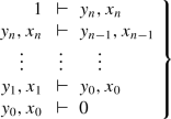
• 2. For any sequence $(x_0,\ldots ,x_n)$ in $\mathbf {T}'$ there exists an integer $k\ge 0$ and elements $a_1,\ldots ,a_k\in \mathbf {T}$ such that for each partition $(H,H')$ of $\{1,\ldots ,k\}$, there exist $y_0,\ldots ,y_n\in \mathbf {T}'$ such that

  $$\begin{aligned} \begin{array}{rclll} \bigwedge _{j\in H'} a_j &{} \,\vdash \,&{} y_n,\;x_n \\ y_n,\;x_n&{} \,\vdash \,&{}y_{n-1},\;x_{n-1} \\ \vdots \qquad &{} \vdots &{} \qquad \vdots \\ y_1,\;x_1&{} \,\vdash \,&{} y_0,\;x_0 \\ y_0,\;x_0&{} \,\vdash \,&{} \bigvee _{j\in H} a_j \\ \end{array} \end{aligned}$$

  (11)

For example, for the relative dimension $n\le 2$, the inequalities in (11) correspond to the following diagram in $\mathbf {T}$, with $u=\bigwedge _{j\in H'} a_j$ and $i=\bigvee _{j\in H} a_j$:

Note that the dimension of the morphism $\mathbf {T}\rightarrow \mathbf {T}'$ is less than or equal to the dimension of $\mathbf {T}'$: take $k=0$ in item 2.

The Krull dimension of a ring $\mathbf {A}$ and of a morphism $\varphi :\mathbf {A}\rightarrow \mathbf {B}$ are those of ${\mathop {\mathsf {Zar}}\nolimits \mathbf {A}}$ and $\mathop {\mathsf {Zar}}\nolimits \varphi$.

A commutative ring $\mathbf {A}$ is zero-dimensional when for each $a\in \mathbf {A}$ there exist $n\in \mathbb {N}$ and $x\in \mathbf {A}$ such that $x^n(1-xa)=0$. A reduced zero-dimensional ring⁹ is a ring in which any element a has a quasi-inverse $b=a^\bullet$, i.e. such that $aba=a$ and $bab=b$.

Let $\mathbf {A}^\bullet$ the reduced zero-dimensional ring generated by $\mathbf {A}$. Then the Krull dimension of a morphism $\rho :\mathbf {A}\rightarrow \mathbf {B}$ equals the Krull dimension of the ring $\mathbf {A}^\bullet \otimes _\mathbf {A}\mathbf {B}$.

3.3 Properties of Spaces

The spectral space ${\mathsf {Spec}\,}\,\mathbf {T}$ is said to be normal if any prime ideal of $\mathbf {T}$ is contained in a unique maximal ideal.

Theorem 11

We have the following equivalences:

• 1. The spectral space ${\mathsf {Spec}\,}(\mathbf {T})$ is normal $\Longleftrightarrow$

  for each $x \vee y = 1$ in $\mathbf {T}$ there exist a, b such that $a \vee x = b \vee y = 1$ and $a \wedge b = 0$.

• 2. In the spectral space ${\mathsf {Spec}\,}(\mathbf {T})$ each quasi-compact open set is a finite union of irreducible quasi-compact open sets $\Longleftrightarrow$

  the distributive lattice $\mathbf {T}$ is constructed from a dynamical algebraic structure where all axioms are Horn rules (e.g. this is the case for purely equational theories).

4 Some Examples

We give in this section constructive versions of classical theorems. Often, the theorem has exactly the same wording as the classical one. But now, these theorems have a clear computational content, which was impossible when using classical definitions. Sometimes the new theorem is stronger than the previously known classical results (e.g. Theorems 17 or 18 or 19).

4.1 Relative Dimension, Lying Over, Going Up, Going Down

See [11] and [17, Section XIII-9].

Theorem 12

Let $\rho :\mathbf {A}\rightarrow \mathbf {B}$ be a morphism of commutative rings or distributive lattices. If $\mathop {\mathsf {Kdim}}\nolimits \,\mathbf {A}\le m$ and $\mathop {\mathsf {Kdim}}\nolimits \,\rho \le n$, then $\mathop {\mathsf {Kdim}}\nolimits \,\mathbf {B}\le (m+1)(n+1)-1$.

Theorem 13

If a morphism $\alpha :\mathbf {A}\rightarrow \mathbf {B}$ of distributive lattices or of commutative rings is lying over and going up (or lying over and going down) one has $\mathop {\mathsf {Kdim}}\nolimits (\mathbf {A})\le \mathop {\mathsf {Kdim}}\nolimits (\mathbf {B})$.

Lemma 4

Let $\rho :\mathbf {A}\rightarrow \mathbf {B}$ be a morphism of commutative rings. If $\mathbf {B}$ is generated by primitively algebraic elements¹⁰ over $\mathbf {A}$, then $\mathop {\mathsf {Kdim}}\nolimits \rho \le 0$ and so $\mathop {\mathsf {Kdim}}\nolimits \mathbf {B}\le \mathop {\mathsf {Kdim}}\nolimits \mathbf {A}$.

Lemma 5

Let $\varphi :\mathbf {A}\rightarrow \mathbf {B}$ be a morphism of commutative rings. The morphism $\varphi$ is lying over if and only if for each ideal $\mathfrak {a}$ of $\mathbf {A}$ and each $x\in \mathbf {A}$, one has $\, \varphi (x)\in \varphi (\mathfrak {a})\mathbf {B}\, \Rightarrow \, x\in \root \mathbf {A} \of {\mathfrak {a}}.$

Lemma 6

Let $\varphi :\mathbf {A}\rightarrow \mathbf {B}$ be a morphism of commutative rings. T.F.A.E.

• 1. The morphism $\varphi$ is going up (i.e. the morphism $\mathop {\mathsf {Zar}}\nolimits \,\varphi$ is going up).

• 2. For any ideal $\mathfrak {b}$ of $\mathbf {B}$, with $\mathfrak {a}=\varphi ^{-1}(\mathfrak {b})$, the morphism $\varphi _\mathfrak {b}:\mathbf {A}/\mathfrak {a}\rightarrow \mathbf {B}/\mathfrak {b}$ is lying over.

• 3. The same thing with finitely generated ideals $\mathfrak {b}$.

• 4. (In classical mathematics) the same thing with prime ideals.

Lemma 7

Let $\mathbf {A}\subseteq \mathbf {B}$ be a faithfully flat $\mathbf {A}$-algebra. The morphism $\mathbf {A}\rightarrow \mathbf {B}$ is lying over and going up. So $\mathop {\mathsf {Kdim}}\nolimits \, \mathbf {A}\le \mathop {\mathsf {Kdim}}\nolimits \, \mathbf {B}$.

Lemma 8

(A classical going up) Let $\mathbf {A}\subseteq \mathbf {B}$ be commutative rings with $\mathbf {B}$ integral over $\mathbf {A}$. Then the morphism $\mathbf {A}\rightarrow \mathbf {B}$ is lying over and going up. So $\mathop {\mathsf {Kdim}}\nolimits \, \mathbf {A}\le \mathop {\mathsf {Kdim}}\nolimits \, \mathbf {B}$.

Lemma 9

Let $\varphi :\mathbf {A}\rightarrow \mathbf {B}$ be a morphism of commutative rings. T.F.A.E.

• 1. The morphism $\varphi$ is going down.

• 2. For b, $a_1$, ..., $a_q\in \mathbf {A}$ and $y\in \mathbf {B}$ such that $\varphi (b)y\in \root \mathbf {B} \of {\left\langle {\varphi (a_1,\ldots ,a_q)}\right\rangle }$, there exist $x_1$, ..., $x_p\in \mathbf {A}$ such that

  $$ \left\langle {bx_1,\ldots ,bx_p}\right\rangle \subseteq \root \mathbf {A} \of {\left\langle {a_1,\ldots ,a_q}\right\rangle } \;\hbox { and }\;y\in \root \mathbf {B} \of {\left\langle {\varphi (x_1), \ldots , \varphi (x_p)}\right\rangle }. $$

• 3. (In classical mathematics) for each prime ideal $\mathfrak {p}$ of $\mathbf {B}$ with $\mathfrak {q}=\varphi ^{-1}(\mathfrak {p})$ the morphism $\mathbf {A}_\mathfrak {q}\rightarrow \mathbf {B}_\mathfrak {p}$ is lying over.

Theorem 14

(Going down) Let $\mathbf {A}\subseteq \mathbf {B}$ be commutative rings. The inclusion morphism $\mathbf {A}\rightarrow \mathbf {B}$ is going down in the following cases:

• 1. $\mathbf {B}$ is flat over $\mathbf {A}$.

• 2. $\mathbf {B}$ is a domain integral over $\mathbf {A}$, and $\mathbf {A}$ is integrally closed.

4.2 Kronecker, Forster–Swan, Serre and Bass Theorems

References: [8, 9] and [17, Chapter XIV].

Theorem 15

(Kronecker–Heitmann theorem, with Krull dimension, without Noetherianity)

• 1. Let $n\ge 0$. If $\mathop {\mathsf {Kdim}}\nolimits \mathbf {A}<n$ and $b_1$, ..., $b_n\in \mathbf {A}$, there exist $x_1$, ..., $x_n$ such that for all $a\in \mathbf {A}$, $\mathrm {D}_\mathbf {A}(a,b_1,\ldots ,b_n) = \mathrm {D}_\mathbf {A}(b_1+ax_1,\ldots ,b_n+ax_n)$.

• 2. Consequently in a ring with Krull dimension $\le n$, every finitely generated ideal  has the same nilradical as an ideal generated by at most $n+1$ elements.

For a commutative ring $\mathbf {A}$ we define $\mathop {\mathsf {Jdim}}\nolimits \mathbf {A}$ (J-dimension of $\mathbf {A}$) as being $\mathop {\mathsf {Kdim}}\nolimits (\mathop {\mathsf {Heit}}\nolimits \mathbf {A})$. In classical mathematics it is the dimension of the Heitmann J-spectrum $\mathop {\mathsf {Jspec}}\nolimits (\mathbf {A})$.

Another dimension, called Heitmann dimension and denoted by $\mathop {\mathsf {Hdim}}\nolimits (\mathbf {A})$, has been introduced in [8, 9]. One has always $\mathop {\mathsf {Hdim}}\nolimits (\mathbf {A})\le \mathop {\mathsf {Jdim}}\nolimits (\mathbf {A})\le \mathop {\mathsf {Kdim}}\nolimits (\mathbf {A})$. The following results with $\mathop {\mathsf {Jdim}}\nolimits$ hold also for $\mathop {\mathsf {Hdim}}\nolimits$.

Definition 4

A ring $\mathbf {A}$ is said to have stable range (of Bass) less than or equal to n when unimodular vectors of length $n+1$ may be shortened in the following meaning:

$$1 \in \left\langle {a,a_1,\ldots ,a_n}\right\rangle \;\Longrightarrow \;\exists \,x_1,\ldots ,x_n,\;1 \in \left\langle {a_1 + x_1a, \ldots , a_n + x_na}\right\rangle .$$

Theorem 16

(Bass–Heitmann Theorem, without Noetherianity) Let $n\ge 0$. If $\mathop {\mathsf {Jdim}}\nolimits \mathbf {A}<n$, then $\mathbf {A}$ has stable range $\le n$. In particular each stably free $\mathbf {A}$-module of rank $\ge n$ is free.

A matrix is said to be of rank $\ge k$ when the minors of size k are comaximal.

Theorem 17

(Serre’s Splitting Off theorem, for $\mathop {\mathsf {Jdim}}\nolimits$)

Let $k\ge 1$ and M be a projective $\mathbf {A}$-module of rank $\ge k$, or more generally isomorphic to the image of a matrix of rank $\ge k$.

Assume that $\mathop {\mathsf {Jdim}}\nolimits \mathbf {A}< k$. Then $M\simeq N\oplus \mathbf {A}$ for a suitable module N isomorphic to the image of a matrix of rank $\ge k-1$.

Corollary 1

Let $\mathbf {A}$ be a ring such that $\mathop {\mathsf {Jdim}}\nolimits \mathbf {A}\le h$ and M be an $\mathbf {A}$-module isomorphic to the image of a matrix of rank $\ge h+s$. Then M has a direct summand which is a free submodule of rang s. Precisely, if M is the image of a matrix $F\in \mathbf {A}^ {n\times m}$ of rank $\ge h+s$, one has $M= N\oplus L$ where L is a direct summand that is free of rank s in $\mathbf {A}^n$, and N the image of a matrix of rank $\ge h$.

In the following theorem we use the notion of finitely generated module locally generated by k elements. In classical mathematics this means that after localisation at any maximal ideal, M is generated by k elements. A classically equivalent constructive definition is that the k-th Fitting ideal of M is equal to $\left\langle {1}\right\rangle$.

Theorem 18

(Forster–Swan theorem for $\mathop {\mathsf {Jdim}}\nolimits$) If $\mathop {\mathsf {Jdim}}\nolimits \mathbf {A}\le k$ and if the $\mathbf {A}$-module $M=\left\langle {y_1 , \ldots , y_{k+r+s}}\right\rangle$ is locally generated by r elements, then it is generated by $k+r$ elements: one can compute $z_1,\, \ldots , \,z_{k+r}$ in $\left\langle {y_{k+r+1},\ldots ,y_{k+r+s}}\right\rangle$ such that M is generated by $(y_1+z_1, \ldots , y_{k+r}+z_{k+r})$.

Theorem 19

(Bass’ cancellation theorem, with $\mathop {\mathsf {Jdim}}\nolimits$)

Let M be a finitely generated projective $\mathbf {A}$-module of rank $\ge k$. If $\mathop {\mathsf {Jdim}}\nolimits \mathbf {A}< k$, then M is cancellative for every finitely generated projective $\mathbf {A}$-module. That is, if Q is finitely generated projective and $M\oplus Q\simeq N\oplus Q$, then $M\simeq N$.

Theorems 17, 18 and 19 were conjectured by Heitmann in [14] (he proved these theorems for the Krull dimension without Noetherianity assumption).

4.3 Other Results Concerning Krull Dimension

In [17] Theorem XII-6.2 gives the following important characterisation. An integrally closed coherent ring $\mathbf {A}$ of Krull dimension at most 1 is a Prüfer domain. This explains in a constructive way the nowadays classical definition of Dedekind domains as Noetherian, integrally closed domains of Krull dimension 1, and the fact that, from this definition, in classical mathematics, one is able to prove that finitely generated nonzero ideals are invertible.

In [17, Chapter XVI] there is a constructive proof of the Lequain–Simis theorem. This proof uses the Krull dimension.

In [24, Section 2.6] we find the following new result, with a constructive proof. If  $\mathbf {A}$ is a ring of Krull dimension $\le d$, then the stably free modules of rank $>d$ over $\mathbf {A}[X]$ are free.

References

Balbes, R., Dwinger, P.: Distributive Lattices. University of Missouri Press, Columbia, Mo (1974)
Bezem, M., Coquand, T.: Automating coherent logic. In: Logic for Programming, Artificial Intelligence, and Reasoning. Proceedings of the 12th International Conference, LPAR 2005, Montego Bay, Jamaica, 2–6 Dec 2005. pp. 246–260. Springer, Berlin (2005)
Bishop, E., Bridges, D.: Constructive analysis. Grundlehren der Mathematischen Wissenschaften [Fundamental Principles of Mathematical Sciences], vol. 279. Springer, Berlin (1985)
Bishop, E.: Foundations of Constructive Analysis. McGraw-Hill, New York (1967)
Borceux, F.: Handbook of Categorical Algebra, Encyclopedia of Mathematics and its Applications, vol. 3, no. 52. Cambridge University Press, Cambridge (1994). Categories of sheaves
Bridges, D., Richman, F.: Varieties of constructive mathematics. London Mathematical Society Lecture Note Series, vol. 97. Cambridge University Press, Cambridge (1987)
Cederquist, J., Coquand, T.: Entailment relations and distributive lattices. In: Logic Colloquium ’98 (Prague). Lecture Note in Logic, vol. 13, pp. 127–139. Association for Symbolic Logic, Urbana, IL (2000)
Coquand, T., Lombardi, H., Quitté, C.: Dimension de Heitmann des treillis distributifs et des anneaux commutatifs. In: Algèbre et théorie des nombres. Années 2003–2006, pp. 57–100. Laboratoire de Mathématiques de Besançon, Besançon, 2006. Revised version in 2017. http://arxiv.org/abs/1712.01958
Coquand, T., Lombardi, H., Quitté, C.: Generating non-Noetherian modules constructively. Manuscripta Math. 115(4), 513–520 (2004)
Coquand, T., Lombardi, H.: A logical approach to abstract algebra. Math. Struct. Comput. Sci. 16(5), 885–900 (2006)
Coquand, T., Lombardi, H.: Constructions cachées en algebre abstraite. Dimension de Krull, Going up, Going down. 2001. Updated version. Technical report, Laboratoire de Mathématiques de l’Université de Franche-Comté (2018). http://hlombardi.free.fr/GoingUpDownFrench-2018.pdf
Coquand, T., Lombardi, H.: Hidden constructions in abstract algebra: Krull dimension of distributive lattices and commutative rings. In: Commutative Ring Theory and Applications (Fez, 2001). Lecture Notes in Pure and Applied Mathematics, Dekker, New York, vol. 231, pp. 477–499 (2003)
Coste, M., Lombardi, H., Roy, M.-F.: Dynamical method in algebra: effective Nullstellensätze. Ann. Pure Appl. Log. 111(3), 203–256 (2001)
Heitmann, R.: Generating non-Noetherian modules efficiently. Mich. Math. J. 31, 167–180 (1984)
Hochster, M.: Prime ideal structure in commutative rings. Trans. Am. Math. Soc. 142, 43–60 (1969)
Johnstone, P.T.: Stone Spaces. Cambridge studies in Advanced Mathematics, vol. 3. Cambridge University Press, Cambridge (1986). Reprint of the 1982 edition
Lombardi, H., Quitté, C.: Commutative algebra: constructive methods. Finite projective modules. Algebra and Applications. Springer, Dordrecht (2015). Translated from the French (Calvage & Mounet, 2011, revised and extended by the authors) by Tania K. Roblot
Lombardi, H.: Dimension de Krull, Nullstellensätze et évaluation dynamique. Math. Z. 242(1), 23–46 (2002)
Lombardi, H.: Structures algébriques dynamiques, espaces topologiques sans points et programme de Hilbert. Ann. Pure Appl. Log. 137(1–3), 256–290 (2006)
Lombardi, H.: Théories géométriques pour l’algébre constructive (2018). http://hlombardi.free.fr/Theories-geometriques.pdf
Lorenzen, P.: Algebraische und logistische Untersuchungen über freie Verbände. J. Symbol. Log. 16, 81–106 (1951). Translation by Stefan Neuwirth: Algebraic and logistic investigations on free lattices. http://arxiv.org/abs/1710.08138
Mines, R., Richman, F., Ruitenburg, W.: A course in constructive algebra. Universitext. Springer, New York (1988)
Stone, M.H.: Topological representations of distributive lattices and Brouwerian logics. Cas. Mat. Fys. 67, 1–25 (1937)
Yengui, I.: Constructive commutative algebra: projective modules over polynomial rings and dynamical Gröbner bases. Lecture Notes in Mathematics, vol. 2138. Springer, Cham (2015)
Author information
Authors and Affiliations
Corresponding author
Editor information
Editors and Affiliations
Rights and permissions
Copyright information
© 2020 Springer Nature Switzerland AG
About this paper
Cite this paper
Lombardi, H. (2020). Spectral Spaces Versus Distributive Lattices: A Dictionary. In: Facchini, A., Fontana, M., Geroldinger, A., Olberding, B. (eds) Advances in Rings, Modules and Factorizations. Rings and Factorizations 2018. Springer Proceedings in Mathematics & Statistics, vol 321. Springer, Cham. https://doi.org/10.1007/978-3-030-43416-8_13
Download citation
DOI: https://doi.org/10.1007/978-3-030-43416-8_13
Published:
Publisher Name: Springer, Cham
Print ISBN: 978-3-030-43415-1
Online ISBN: 978-3-030-43416-8
eBook Packages: Mathematics and StatisticsMathematics and Statistics (R0)