Electrophysiological Mapping and Source Imaging

Abstract

In this chapter, we present the physical and physiological basics behind EEG and MEG signal generation and propagation. We first start by presenting the biophysical principles that explain how the coordinated movements of ions inside and outside neuronal cells result in macroscale phenomena at the scalp, such as electric potentials recorded by EEG and magnetic fields sensed by MEG. These physical principles enforce EEG and MEG signals to have specific spatial and temporal features, which can be used to study brain’s response to internal and external stimuli. We continue our exploration by developing a mathematical framework within which EEG and MEG signals can be computed if the distribution of underlying brain sources is known, a process called forward problem. We further continue to discuss methods that attempt the reverse, i.e., solving for underlying brain sources given scalp measurements such as EEG and MEG, a process called source imaging. We will provide various examples of how electrophysiological source imaging techniques can help study the brain during its normal and pathological states. We will also briefly discuss how combining electrophysiological signals from EEG with hemodynamic signals from functional magnetic resonance imaging (fMRI) helps improve the spatiotemporal resolution of estimates of the underlying brain sources, which is critical for studying spatiotemporal processes within the brain. The goal of this chapter is to provide proper physical and physiological intuition and biophysical principles that explain EEG/MEG signal generation, its propagation from sources in the brain to EEG/MEG sensors, and how this process can be inverted using signal processing and machine learning techniques and algorithms.

13.1 Introduction

13.1.1 Generation and Measurement of EEG and MEG

Although electrical activity recorded from the exposed cerebral cortex of a monkey was reported in 1875 [1], it was not until 1929 that Hans Berger, a psychiatrist in Jena, Germany, first recorded noninvasively rhythmic electrical activity from the human scalp [2], which has subsequently known as electroencephalography (EEG). Since then, EEG has become an important tool for probing brain electrical activity and aiding in clinical diagnosis of neurological disorders, due to its excellent temporal resolution in the order of millisecond. The first recording of magnetic fields from the human brain was reported in 1972 by David Cohen at the Massachusetts Institute of Technology [3], which led to the development of magnetoencephalography (MEG). Like EEG, MEG also enjoys high temporal resolution in detecting brain electrical activity. EEG and MEG have become two prominent methods for noninvasive assessment of brain electrical activity, providing unsurpassed temporal resolution, in neuroscience research and clinical applications.

EEG and MEG are considered to originate from, in principle, the same brain electrical activity, which are current flows caused by neuronal excitation. The discharge of a single neuron or single nerve fiber in the brain generates an extremely small electric potential or magnetic field, which cannot be observed over the scalp due to the background noise.

Instead, the externally recorded EEG and MEG represent the summation of the electric potentials and magnetic fluxes generated by many thousands or even millions of neurons or fibers when they fire synchronously [4]. In other words, the intensities of EEG and MEG signals are determined mainly by the number of neurons and fibers that fire in synchrony. An anatomic structure in the human brain, which favors the neuronal synchrony and summation of electric potentials or magnetic fields from neuronal synchrony, is the cortex, which is also in the vicinity to the scalp where electrical or magnetic sensors are placed. Due to the separation of the apical and basal dendrites in pyramidal cells, a considerable distance exists between the current sources and sinks, resulting in strong current dipoles as perceived by EEG and MEG [5]. Additionally, these cells are arranged in parallel to each other and perpendicular to the cortical surface, in an arrangement referred to as the palisade which constructively adds the effect of smaller current dipoles from individual cells together, to effectively constitute a strong current dipole [6]. It is thus believed that EEG and MEG predominantly detect synchronized current flows in the cortical pyramidal neurons, which are laid out perpendicularly to the convoluted cortical sheet of gray matter [7]. This is schematically shown in Fig. 13.1.

Fig. 13.1

Electrophysiological principles of current dipoles. Macroscopic phenomena, such as the electric potential recorded at scalp EEG or magnetic field recorded at MEG sensors, are due to the summation of many microscopic quantities such as postsynaptic potentials of pyramidal cells

Dipole models are used more frequently (compared to monopoles and multipoles [7, 8]) to describe the underlying biophysics of neural activity, as they provide an easier physical interpretation of the underlying phenomenon and can be viewed as an approximate discrete representation of current density at a mesoscopic level. Furthermore, the electromagnetic fields generated by multipoles attenuate much faster with distance, compared to dipoles, inadvertently resulting in dipole fields dominating EEG and MEG measurements [8, 9]. This is supported by the fact that the distance between current sources and sinks is almost neglectable as compared with their distances to the locations where EEG and MEG signals are being recorded.

The intensities of the scalp EEG range from 0 to 200 μV, which fluctuate mainly in the frequency range of up to 50 Hz. The EEG recording involves the application of a set of electrodes to standard positions on the scalp. The most commonly used electrode placement montage is the international 10–20 system, which uses the distances between bony landmarks of the head to generate a system of lines which run across the head and intersect at intervals of 10% or 20% of their total length. Additional electrodes can also be introduced according to expanded 10–20 systems as proposed by the American EEG Society. Most clinical EEG recordings are up to 32 electrodes, while merits of high-density EEG recordings have been reported by multiple studies [4, 10]. A recent recommendation from the working group of the International Federation of Clinical Neurophysiology suggests using 64 electrodes or more for source imaging and localization [11].

The difficulty in recording magnetic fields from the human brain is its strengths that are weaker than couple of pico-Tesla (pT), which is about 10⁸ times less than the earth’s geomagnetic field. MEG recordings were made available due to the invention of a sensitive magnetic flux detector, known as the superconducting quantum interference device (SQUID) [7] (Fig. 13.2). The frequency range of MEG is similar to EEG, which is between 0 and 50 Hz.

Fig. 13.2

Schematics of MEG instrumentation. A single-channel axial gradiometer and associated SQUID inside a dewar filled with liquid helium. The bottom depicts the sensor array of a 306-channel MEG helmet where each sensor unit contains two orthogonal planar gradiometers and one magnetometer. (From [20], licensed under CC BY 4.0)

While most analysis performed in EEG and MEG is within the 0–50 Hz band due to the high concentration of energy within these bands, high-frequency oscillations (HFOs) have been successfully detected and analyzed in scalp recordings [12,13,14]. HFOs are typically observed in intracranial recordings and can span a frequency band of 30–600 Hz and are thought to be involved in physiological processes such as attention, learning, and memory, as well as pathological processes such as ictogenesis [13]. HFOs, typically in the range of 80–250 Hz, have been ubiquitously and reliably observed and reported in scalp recordings, in the recent years [15, 16]. Not only have these events been reliably detected in noninvasive scalp measurements, but also HFOs are traced back to the source space and shown to correlate well with clinical findings determining the seizure onset in epilepsy patients [15], encouraging researchers and clinicians to consider HFOs as a potential biomarker for ictogenesis [17]. While this view has been modified recently [18], HFOs can be reliably detected in EEG and MEG, emphasizing that broad spectral information can be extracted in noninvasive recordings as well [6].

In recording systems, while the number of MEG sensors used is usually different from EEG, the spatial coverage and layout of MEG sensors are similar to those for EEG, which are distributed over a surface in parallel to the scalp surface (Fig. 13.2). MEG sensors are not necessary to touch the scalp due to the magnetic permeability of air, which is also different from EEG. On the other hand, since the magnetic fields from the human brain are extremely weak compared with ambient magnetic fields, MEG recording systems are much more complicated than EEG recording systems. The SQUID system is commonly designed not to be sensitive to uniform background magnetic fields using gradiometers, and MEG recordings are usually conducted in a magnetically shielded room. Recently the feasibility of a wearable MEG system was reported for human use [19], although this technology is still under development and is currently quite expensive.

In both EEG and MEG signals recorded over the human head, the major constituents are those contributed by spontaneous brain electrical activity and potentials and/or magnetic fields evoked by external stimuli/events, known as the evoked potentials and/or (magnetic) fields or event-related potentials and/or fields (ERPs/ERFs). Since external stimuli/events can be specifically designed to evoke targeted functional areas, such as visual, auditory, and somatosensory cortices, associated measurements have thus been widely practiced to study the functions of these areas. Correspondingly, evoked potentials and/or fields are the visual evoked potential/field (VEP/VEF), auditory evoked potential/field (AEP/AEF), and the somatosensory evoked potential/field (SEP/SEF).

13.1.2 Spatial and Temporal Resolution of EEG and MEG

Brain electrical activation is a spatiotemporal process, which means that its activity is distributed over three dimensions and evolves in time. The most important merit of EEG and MEG is their unsurpassed millisecond-scale temporal resolution. This feature is essential for resolving rapid change of neurophysiological process, considering the typical temporal scale of neuronal electrical events which is from one to several tens of milliseconds. However, both EEG and MEG are limited by their spatial resolutions.

The conventional EEG has limited spatial resolution mainly due to two factors. One factor is the limited spatial sampling. A remarkable development in the past decades is that high-resolution EEG systems with 64–256 electrodes have been commercially available. For example, with up to 124 scalp electrodes, the average inter-electrode distance can be reduced to about 2.5 cm [10, 21]. The multichannel SQUID system was challenged initially due to the complexity of superconductive coils that were necessary to be sensitive to weak brain magnetic signals [7]. Nowadays, multichannel SQUID systems have been commercially available too. The second factor is the head volume conduction effect. The electric potentials generated from neural sources are attenuated and blurred as they pass through the neural tissue, cerebrospinal fluid, meninges, low-conductivity skull, and scalp [9]. While the magnetic fields are also suffered from the volume conduction effect as for its attenuation and spatial smoothness, MEG is practically unaffected by the low-conductivity skull.

Advanced EEG and MEG imaging techniques are highly desired in order to compensate for the head volume conduction effect and enhance the spatial resolution of scalp EEG and MEG. The solutions of two separate but closely related problems, EEG/MEG forward problem and EEG/MEG inverse problem, are required for imaging of brain electric activity based on external potential and/or field measurements.

13.2 Electrophysiological Mapping

13.2.1 EEG Mapping

Due to the fast response of EEG/MEG to neural events, a major use of EEG/MEG signals is to make observations in their time courses [22, 23]. Plenty of temporal components have been well defined and widely accepted in various paradigms. For example, N100 component is a negative-going deflection from baseline in AEPs (its equivalent in MEG is the M100 [7]), which peaks at the latency of about 100 ms after the onset of an auditory stimulus. In VEP, multiple temporal (either positive- or negative-going) components at different latencies have been identified in a sequence after a visual stimulus. The dynamics of these temporal components and their latencies indicate the important information about the timings and sequences of neuronal processes in response to specific stimuli.

Other than time information, efforts have been made to obtain spatial information with regard to the underlying brain electrical activity. Figure 13.3 shows an example of scalp EEG maps during a binocular rivalry paradigm [22]. Strong counterphase modulations are revealed in EEG maps for attended rivalry, and the scalp EEG maps also suggest occipital origin of sources responsible for the scalp EEG during binocular rivalry. EEG mapping is to visualize potential values from different electrodes measured at the same time instance on the scalp surface. Since EEG recordings can only be obtained in locations where electrodes are placed, potential values in inter-electrodes areas are usually interpolated, mainly using linear methods, for higher-resolution visualization. The assumption behind linear interpolations is the smooth transition of potential values among neighbored electrodes. However, the accuracy of interpolations also depends on the number of electrodes. Figure 13.4a, b illustrates an example of scalp EEG maps interpolated using measurements from 32 channels and 122 channels, respectively. The scalp EEG map in Fig. 13.4a is smoother with reduced peak values and sharper transitions than the scalp EEG map from Fig. 13.4b. These problems are caused by the low-density samples from a fewer number of electrodes, which leads to large inter-electrode distances. Nonlinear interpolations can also be used, such as spline interpolation [24]. An example of spline interpolation can be found in applications where a continuous function of an EEG map is necessary, such as for the calculation of a surface Laplacian EEG map.

Fig. 13.3

Time courses of scalp EEG power maps. These scalp topographies show power at the tagged frequencies at each electrode, as averaged over a group of subjects. Seven maps were drawn for each 6 s epoch. In each of the four panels, the upper row shows power for the aligned eye’s frequency, and lower row shows power for the time-locked signal from the other eye. Inset line graphs show the results from occipital electrodes. Both line graphs and topographies show strong counterphase modulations, except in the unattended rivalry condition. (From Zhang et al. [22] with permission)

Fig. 13.4

Simulated EEG data and MEG data under different conditions. (a) The scalp EEG map generated by a tangential dipole using low-density 32 electrodes. (b) The high-density scalp EEG (left) from 122 electrodes and MEG (middle) from 151 sensors generated by a tangential dipole on the cortical surface (right). (c) The high-density scalp EEG (left) from 122 electrodes and MEG (middle) from 151 sensors generated by a radial dipole on the cortical surface (right)

To illustrate EEG maps, two visualization tools are usually used, contour lines, in which each line connects isopotential points on the scalp, or pseudo-colors (which are more common), in which each color represents a potential value. Figure 13.4 shows EEG maps using pseudo-colors. Along the direction of current flow within the brain source area (indicated by the red arrow in figures), potentials are positive. A symmetric negative pattern is usually accompanied in the opposite direction of current flow (Fig. 13.4a, b). Note that EEG measurements are usually made against a reference. While the symmetric pattern along the direction of current flow always exists, whether potential values are positive or negative also depends on the selection of reference.

The scalp EEG maps in both Fig. 13.4a, b are generated by a simulated current dipole source (Fig. 13.4b, right column) via solving the forward problem. A scalp EEG map generated by a small brain source (modeled by a current dipole) can extend about centimeters in diameters over the scalp surface, which is caused by the so-called volume conductor effect. Although the head volume conductor effort causes a smoothed version of spatial distribution of EEG corresponding to the brain electric sources, EEG mapping represents an easy and fast tool to assess the global nature of brain electric activity (e.g., frontal lobe vs. occipital lobe, see also Fig. 13.3 for visual events).

13.2.2 MEG Mapping

The concept of MEG mapping is similar to EEG mapping except that MEG signals are used instead of EEG signals. In MEG, positive values indicate the outflow of magnetic flux coming at the recording sensor location and negative values indicate the inflow of magnetic flux at that particular location. It is worthwhile to note that MEG signals do not depend on references like EEG and have different sensitivity profiles [25] compared to EEG. Examples of MEG maps are shown in Fig. 13.4b, c (the middle columns) using the same simulated brain sources as for EEG in the same figure. MEG maps also suffer from the volume conductor effect. However, since the magnetic permeability of the skull is similar to other brain tissues, the low-conductivity skull layer affects MEG less. Another property of MEG is that it is not sensitive to radially oriented cortical sources [7]. Figure 13.4 illustrates an example of MEG map generated by a brain source on the ridge of a cortical fold that is close to radial orientation. Its MEG signals are ten times less than MEG signals from a tangential source (Fig. 13.4b). Both EEG and MEG are less sensitive to deeper sources, with MEG being notably insensitive to deeper sources [26]. However, these structural limitations do not necessarily mean EEG, and MEG cannot detect any deep sources. Recent studies with concurrent intracranial and EEG/MEG recordings have provided evidence to the contrary; electromagnetic activity from subcortical regions in the thalamus, amygdala, and hippocampus was unequivocally recorded at EEG and MEG [27, 28]. Seeber et al. showed that the envelope of alpha-wave activity from sources as deep as the centromedian nuclei of the thalamus (direct electrical recordings from deep brain stimulation electrodes placed in these regions) can be recorded in high-density scalp EEG recordings (256 channels) [27]. Furthermore, it was shown that these activities can be traced back to deep source regions by solving the inverse problem. Additionally, Pizzo et al. showed that interictal spikes observed by stereo-EEG (sEEG) electrodes implanted near the amygdala and hippocampus can be detected in MEG recordings by means of blind source separation techniques [28]. Additionally, signals reaching the surface measurements from these deep sources can still be localized to these subcortical structures using source imaging techniques [27, 28].

It is important to understand the difference between EEG and MEG maps since both reflect the common brain activity while each of them has better sensitivity on different aspects of the common brain activity. The electrical field gradient reaches the highest along the direction of current flow of the brain source (indicated by the red arrow in figures), while the magnetic field has the highest gradient across the direction of current flow. Thus, the symmetric field pattern of MEG is on the both side of the arrow, while the symmetric field pattern of EEG appears on the tail and head of the arrow. It is therefore expected that the transverse features of brain sources are more precisely estimated with MEG and the longitudinal features of brain sources are more precisely estimated with EEG. Furthermore, MEG is not sensitive to radial brain sources as discussed earlier, whereas EEG is sensitive to brain sources of all orientations (e.g., comparing Fig. 13.4).

In summary, while the EEG and MEG mapping can provide spatial patterns about brain activity on the scalp, they are limited by their inherited low spatial resolution. The spatial locations of those temporal components of interests can only be referred at the scalp surface according to beneath lobular or sublobular organizations. Significant improvement of spatial resolution of EEG/MEG can be accomplished by source imaging from scalp EEG or MEG.

13.2.3 Surface Laplacian Mapping

In parallel to the development of the source imaging methods to enhance spatial resolution of EEG and MEG, another surface mapping technique, surface Laplacian (SL), has been developed for the similar purpose. The SL does not need to solve the inverse problem as discussed below, nor does it require a forward volume conductor model. Instead, it applies a spatial Laplacian filter (second spatial derivative) to compensate for the head volume conduction effect and achieves high-resolution surface mapping directly over the scalp surface.

The SL has been considered as an estimate of the local current density flowing perpendicular to the skull into the scalp; thus it has also been termed current source density or scalp current density [29]. The SL has also been considered as an equivalent surface charge density corresponding to the surface potential [30]. Compared to the EEG source imaging approaches, the SL approach does not require exact knowledge about the source models and the volume conductor models and has unique advantage of reference independence.

Since Hjorth’s early exploration on scalp Laplacian of EEG [31], many efforts have been made to develop reliable and easy-to-use SL techniques. Of note are the developments of spherical spline SL [29] and the realistic geometry spline SL [24, 32]. Bipolar or tripolar concentric electrodes have also been used to measure the SL. He and colleagues proposed to use the bipolar concentric electrode to record the SL [30] under the assumption that the outer ring of the concentric electrode would provide reasonable estimate of the averaged potential over the surrounding ring [30]. A tripolar concentric ring electrode has also been used to measure SL [33]. The SL has been widely used in EEG-based brain-computer interface to improve signal quality of measurements associated with intentions.

13.2.4 Multivariate Pattern Analysis of EEG and MEG Signals

The brain encodes the information it receives and processes into neural codes, which, inadvertently, manifest themselves as neural patterns of activity. The neuronal activity, consequently, leaves an electromagnetic footprint that gets picked up by EEG and MEG [4]. A great deal of studies and investigations are conducted to decode these patterns and extract such information. Multivariate pattern analysis or MVPA is the general term used to describe the process of analyzing signals gathered from many neurons and brain regions to differentiate between different brain states to ultimately understand how the brain encodes information [34]. MVPA can be thought of as supervised learning, to put in machine learning language, which learns spatial patterns of neuronal activity over different cognitive conditions or external stimuli. This technique has been applied to MEG and EEG measurements at scalp, prior to solving the inverse problem [35], and at source space, after solving the inverse [36]. MVPA can be thought of as a systematic approach to mapping spatiotemporal neural activity to brain states and cognitive conditions, in continuation of what was discussed above.

MVPA is capable of detecting complex spatial neural patterns as experimental conditions or external stimuli can be repeated many times to ensure the statistical integrity of the data. This technique has been applied recently to MEG and EEG measurements for studying object recognition, face perception, and memory [35]. These studies not only benefited from spatially rich information contained in EEG and MEG measurements but also took advantage of the high temporal resolution of the aforementioned modalities to further understand when different brain processes occur in the brain with respect to each other; for instance, Linde-Domingo et al. showed that during seeing objects, low-level visual features could be decoded faster than high-level conceptual features [35]. The reverse was true for associative memory recall. Therefore, applying MVPA to EEG and MEG could provide a spatiotemporal decoding scheme which ultimately leads to the better understanding of the brain.

13.3 EEG/MEG Forward Modeling

Given the known information on brain electric source distribution (i.e., source models) and head volume conduction properties (i.e., volume conductor models), EEG and MEG forward problems determine the source-generated electric potential and magnetic field (Fig. 13.4). Note that while the EEG forward solution mainly refers to electric potentials, such as the cortical potential or the scalp potential, it can also be other metrics, for example, the surface Laplacian. In MEG, the forward solution is usually referred to as magnetic fields. Since magnetic fields are vector fields, the forward solution can be referred as a component of magnetic fields, such as radial or tangential component. Furthermore, since most MEG systems use gradiometers, the MEG forward solution can be magnetic gradient fields or second-order gradient fields. Both EEG and MEG forward problems are well defined and have a unique solution, governed by the quasi-static approximations of Maxwell’s equations, that is, Poisson’s equation [8, 9, 37].

By solving the EEG and MEG forward problems, the relationship between neuronal sources and external sensor measurements can be established. In particular, for a given source distribution, EEG and MEG measurements and underlying brain electric sources can be related by the so-called transfer matrix or lead field matrix, which is only dependent on the geometry and electrical properties of the head volume conductor.

13.3.1 Source Models

Several source models have been proposed to equivalently represent brain electric sources. The primary bioelectric sources can be represented as an impressed current density J, which is driven by the electrochemical process of excitable cells in the brain. In other words, it is a nonconservative current that arises from the bioelectric activity of nerve cells due to the conversion of energy from chemical to electrical form [37].

The simplest brain electric source model is a monopole source. In the monopole model, a volume source with ignorable size is considered as a point current source of magnitude I _v lying in a conducting medium, with its current flow lines radially directed in all directions. However, in a living system, only a collection of positive and negative monopole sources is physically realistic as the total sum of currents is zero due to electrical neutrality. The simplest collection of monopole sources is a dipole, which consists of two monopoles of opposite sign, but equal strength, separated by an infinitely small distance. In such a dipole model, its current flow lines start from the positive pole of the source and end at the associated negative pole. The dipole model is the most commonly used model in EEG/MEG source imaging techniques.

Until now, we have only considered the equivalent source models for the impressed current density, which are generated by excitable cells. In order to solve the EEG/MEG source imaging problems, a global equivalent source distribution model should also be determined which can account for the electric activity within the entire brain. State-of-the-art source models usually consist of a source distribution to reflect the distributed nature of electric sources associated with neuronal excitation. Once such a source distribution model is defined, the source imaging solutions can only be searched over the space confined to the distribution model, hence, also known as the source space or solution space. Source models, including the dipole model (which can be viewed as a special case of a source distribution) and the source distribution model, are generally used for both EEG/MEG forward and inverse problems. There are mainly two types of source models, i.e., parametric dipole models [38] and distributed source models [39,40,41]. The parametric dipole models use the ideal equivalent dipole model (ECD) to represent focal electrical activity. In parametric dipole models, multiple ECDs are also used to model multiple focal sources over different brain regions. The distributed source models are more suitable in characterizing extended sources in which the source space is represented by continuously distributed dipole elements over a volume (i.e., the brain) [39, 41] or a surface (i.e., the cortical surface) [40].

The source models are not limited to model electrical currents but may be electric potentials over the cortical surface [21, 42] or within the 3D brain volume [43].

13.3.2 Volume Conductor Models

The volume conductor models are developed to model the human head, which sits between brain sources and EEG/MEG sensors. In order to build these models, the geometry and conductivity or permeability profiles are crucial for EEG or MEG. Early works used spherical head models as closed solutions for EEG/MEG forward problems. The single-sphere model represents the simplest approximation of the head geometry. The three-layer concentric spherical model [44] has been well used to represent compartments of the skin, the skull, and the brain in head volume conductor. Such a model was essentially developed to consider the skull layer since it has significant low-conductivity layer as compared with the skin and the brain. An important development in the field was to incorporate anatomic constraint into EEG/MEG source imaging by developing approaches which could take the realistic head geometry into consideration. He et al. proposed the use of realistic geometry head models for EEG source localization by applying the boundary element method (BEM) [38]. Hämäläinen and Sarvas [45] further developed BEM-based approach to model the head volume conductor for MEG/EEG incorporating the low-conductivity skull layer in addition to the scalp and brain. Several BEM approaches have been developed to solve the head forward problem using a multiple layer realistic geometry model [45, 46]. Here, the multiple layers again refer to the interfaces between the skin, the skull, and the brain, which are similarly represented in three-layer concentric spherical model, but of realistic geometries. The realistic geometries can be obtained by segmenting brain tissues from magnetic resonance (MR) structural images. In addition to the boundary element method, the finite element method (FEM) has also been used to model the head volume conductor [47, 48] in which each finite element can be assigned with a conductivity value or even a conductivity tensor that represents different conductivity values along different directions in a 3D space (known as the anisotropy) [49, 50].

While the aforementioned discussion applies to MEG, as well, in practice, the volume conductor models for MEG are much simpler than those for EEG. The major reason is that the permeability profile for MEG is almost uniform for all brain tissues including the skull. Thus, a volume conductor model with realistic shape for the brain may be sufficient for the forward calculation of MEG signals [7]. In practice, one-sphere model with a similar size to the subject’s head is used, occasionally.

13.3.3 Forward Solutions

Once the volume source model and volume conductor model are selected, the forward solutions can be calculated uniquely. Here we discuss two cases of forward solutions: monopoles and dipoles in infinite homogeneous medium. While these represent the simplest cases for the calculation of forward solutions, which might not be quite realistic in real applications, it can help readers understand the concepts such as the volume conductor effect. Other advanced methods in calculating forward solutions, such as piece-wise homogeneous realistic geometry models or inhomogeneous realistic geometry models, can be found in the literature [45, 48].

If the volume conductor is infinite and homogeneous with conductivity of σ, the bioelectric potential obeys Poisson’s equation under quasi-static conditions [37]:

$$ {\nabla}^2\Phi =\frac{\nabla \cdot {\overset{\rightharpoonup }{J^i}}}{\sigma }=-\frac{I_v}{\sigma } $$

(13.1)

Equation 13.1 is a partial differential equation satisfied by the electric potential Φ in which I _v is the source function. The solution of Eq. 13.1 for the scalar function Φ for a region that is uniform and infinite in extent is [37]:

$$ \Phi =-\frac{1}{4\pi \sigma}{\int}_V\left(\frac{1}{r}\right)\nabla \cdot {\overset{\rightharpoonup }{J^i}} dv $$

(13.2)

where r refers to the distance from the source to the observation point. Since the source element $\nabla \cdot {\overset{\rightharpoonup }{J^i}}\, dv$ in Eq. 13.2 behaves like a point source, in that it sets up a field that varies as 1/r, the expression ${I}_v=-\nabla \cdot {\overset{\rightharpoonup }{J^i}}$ can be considered as an equivalent monopole source [8, 37, 51].

Using the identity $\nabla \cdot \left({\overset{\rightharpoonup }{J^i}}/r\right)=\nabla \left(1/r\right)\cdot {\overset{\rightharpoonup }{J^i}}+\left(1/r\right)\nabla \cdot {\overset{\rightharpoonup }{J^i}}$ and the divergence (or Gauss’s) theorem, Eq. 13.2 can be transformed to [8]:

$$ \Phi =\frac{1}{4\pi \sigma}{\int}_V\nabla \left(\frac{1}{r}\right)\cdot {\overset{\rightharpoonup }{J^i}} dv $$

(13.3)

Here, the source element ${\overset{\rightharpoonup }{J^i}}\,dv$ behaves like a dipole source, with a field that varies as 1/r. Therefore, the impressed current density may be interpreted as an equivalent dipole source. Although higher-order equivalent source models such as the quadrupole can also be studied to represent the bioelectric sources, the dipole model has been so far the most commonly used brain electric source model.

Similar to electric potential, the magnetic field due to a monopole or dipole current source in an infinite homogeneous medium can be derived based on Poisson’s equation. Interested readers can consult the details in [8].

If the three compartments (the brain, skull, scalp) are considered and their surfaces are of realistic shapes, it becomes a realistic geometry piecewise homogeneous model. This is a reasonable approximation for the electrical conductivity profile of the human head modeling the scalp, skull, and brain. The forward solution becomes a sum of the electric potential/magnetic field in the infinite homogeneous medium with a second term that reflects the effect of conductivity inhomogeneity between different compartments [8]. The piecewise homogeneous model and its solution can be generalized to more complicated inhomogeneous model since an inhomogeneous volume conductor can be divided into a finite number of homogeneous regions. A boundary element method algorithm [45] has been introduced to accurately calculate electrical potential and magnetic fields in piecewise homogeneous head volume conductor model.

13.4 EEG/MEG Source Imaging

Given the known electrical potential or magnetic field (e.g., scalp EEG or MEG measurement) and head volume conductor properties, the EEG/MEG source imaging reconstructs the distribution of electric sources within the brain (source space) corresponding to the measured EEG/MEG (Fig. 13.5). A solution to the EEG/MEG source imaging problem thus provides desirable information with regard to the brain electric activity, such as locations or extent of current sources, which can be directly related to the underlying neural activation. Although the EEG/MEG inverse problem is technically challenging, work conducted in the past few decades has indicated that the EEG/MEG source imaging problem can be solved with reasonable resolution and accuracy by incorporating various a priori information, such as anatomic constraints on the sources [40, 41], on volume conductor [38, 45], or functional constraints provided by other imaging modalities such as functional MRI [52,53,54].

Fig. 13.5

Schematic diagram of EEG/MEG electrophysiological neuroimaging. The scalp EEG/MEG is recorded using multichannel data acquisition system. The realistic geometry head volume conductor model can be constructed from the structure MRI of the subject, and the lead field matrix can be modeled using numerical techniques such as BEM or FEM, i.e., forward problem. By solving the inverse source imaging problem, brain electric sources are estimated over the cortex or throughout the brain volume with substantially enhanced spatial resolution as compared with scalp EEG/MEG. (From He et al. [4] with permission)

EEG/MEG source imaging solutions require a source model. The choice of source models depends on particular applications, while the primary goal of EEG/MEG source imaging problems remains the same: to find an equivalent representation of brain electric sources that can account for external EEG/MEG measurements.

13.4.1 Dipole Source Localization

The most commonly used brain electric source model is the equivalent current dipole (ECD) model, which assumes that the scalp EEG or MEG is generated by one or a few focal dipole sources. Each of the focal sources can be modeled by an ECD with six parameters: three location parameters and three dipole-moment parameters. In MEG, since it is less sensitive to radial sources, parameter for radial orientation might be omitted, which leads to five parameters for an ECD.

The simplest and representative ECD model is the single moving dipole, which has varying magnitude and orientation, as well as variable location. The location of the single moving dipole estimates the center of gravity of brain electric activity, which can be informative for focal brain activation, such as origin of focal epileptic activity. The multiple dipole model includes several dipoles, each representing a certain anatomical region of the brain. These dipoles have varying magnitudes and varying orientations, while their locations could be either fixed or variable (i.e., multiple moving ECD models). Due to finite signal-to-noise ratio of the EEG/MEG recordings, the number of multiple dipoles that can be reliably estimated is limited, usually no more than two dipoles in moving dipoles model [55].

Given a specific dipole source model, the dipole source localization (DSL) solves the EEG or MEG inverse problem by using a nonlinear multidimensional minimization procedure, to estimate the dipole parameters that can best explain observed scalp potential or magnetic field measurements in a least-square sense [38, 55,56,57,58]. Further improvement of the DSL can be achieved by combining EEG with MEG data which may increase information content and improve the overall signal-to-noise ratio [59, 60]. Generally speaking, there are two DSL approaches. One approach is the single time-slice source localization, in which the dipole parameters are fitted at a time instance, based on single time “snapshots” of measured scalp EEG or MEG data [38, 58]. For example, scalp potentials or magnetic fields at a single time-slice could be controlled into column vector ϕ, each row of which is electric potential or magnetic field data recorded from one sensor. The problem then is to find a column vector X, the collection of potentials or magnetic fields at the same sensor sites but generated by assumed sources inside the brain. In practice, an initial starting point (also termed seed point) is estimated, and then using an iterative procedure, the assumed dipole sources are moved around inside the brain (the source space) in an attempt to produce the best match between ϕ (measured scalp potential/field) and ψ (scalp potential/field generated by X). This involves solving the forward problem repetitively and calculating the difference between measured and estimated data vectors at each step. The most commonly used measure is the squared distance between the two data vectors, which is given by:

$$ J={\left\Vert \overset{\rightharpoonup }{\phi }-\overset{\rightharpoonup }{\psi}\right\Vert}^2 $$

(13.4)

where J is the objective function which is to be minimized. From Eq. 13.3, it can be known that the relationship between the dipole location (r) and electric potential is nonlinear, and thus the problem expressed in Eq. 13.4 needs to be solved via nonlinear optimization. Different methods could be applied to solve this nonlinear optimization problem, such as the simplex method [38], due to its simplicity and relative robustness to local minima. The nonlinear nature of DSL holds for MEG source localization, as well.

Another approach is the multiple time-slice source localization, also termed spatiotemporal source localization, which incorporates both the spatial and temporal components of the EEG in model fitting [56]. In this approach, multiple dipole sources are assumed to be fixed on unknown locations inside the brain during a certain time interval, and the variations in scalp potentials or magnetic fields are due only to variations in the strengths and orientations of these sources. The dipole sources S can be related to the scalp potentials or magnetic fields, denoted as Φ, by the lead field matrix A, which is only dependent on the head volume conductor properties and the source-sensor configurations:

$$ \overset{\rightharpoonup }{\Phi}=A\overset{\rightharpoonup }{S} $$

(13.5)

Here, Φ is the N channels by T time-slices EEG/MEG data matrix, and S is the M dipoles by T time-slices source waveform matrix. The task of the spatiotemporal DSL is to determine the locations of multiple dipoles [56], whose parameters could best account for the spatial distribution as well as the temporal waveforms of the scalp EEG/MEG measurement. Similar to Eq. 13.4, an iterative procedure is needed to adjust source parameters with the aim to minimize the following objective function:

$$ J={\left\Vert \overset{\rightharpoonup }{\Phi}-A\overset{\rightharpoonup }{S}\right\Vert}^2={\left\Vert \left(I-{AA}^{+}\right)\overset{\rightharpoonup }{\Phi}\right\Vert}^2 $$

(13.6)

where I is the identity matrix and A ⁺ is the pseudo-inverse of matrix A. At each iterative step, locations and orientations of sources are updated which subsequently causes the update of J. Once the product between A and its pseudo-inverse becomes close to I, optimal source locations and orientations are found since the objective function is minimized. With the incorporation of the EEG/MEG temporal information in the model fitting, the spatiotemporal DSL is more robust against measurement noise and artifacts than the single time-slice DSL.

All DSL algorithms need an a priori knowledge of the number and class of the underlying dipole sources. If the number of dipoles is underestimated for a given model, then the DSL inverse solution is biased by the missing dipoles. On the other hand, if too many dipoles are specified, then spurious dipoles can be introduced, which maybe indiscernible from the true dipoles. Moreover, since the computational complexity of the least-squares estimation problem is highly dependent on the number of nonlinear parameters that must be estimated, too many dipoles also add needless computational burden and may not lead to reliable solutions.

In practice, the principal component analysis (PCA) and multiple signal classification (MUSIC) algorithms have been used to approximately estimate the number of field patterns contained in the scalp EEG/MEG data [61]. For example, the MUSIC algorithm scans through the 3D brain volume (solution space) to identify sources that produce potential patterns that lie within the signal subspace of the EEG/MEG measurements [61]. To localize brain electric sources, a linearly constrained minimum variance (LCMV) beamformer approach [62] has been developed for EEG/MEG source localization, by designing a bank of narrow-band spatial filters where each filter passes signals originating from a specified location represented by a dipole within the brain while attenuating signals from other locations. Furthermore, statistical parametric maps based on beamformers can be created by looking at output changes of spatial filters’ comparing conditions, such as between the resting and the task, over the entire brain.

13.4.2 Cortical Potential Imaging

The cortical potential imaging (CPI) technique employs a distributed source model, in which the equivalent sources are distributed in two-dimensional (2D) cortical surface, and no ad hoc assumption on the number of source dipoles is needed as in dipole source localization. This group of techniques is mostly deployed with EEG signals. Using an explicit biophysical model of the passive conducting properties of a head, the CPI attempts to deconvolve a measured scalp potential distribution into a distribution of the electrical potential over the epicortical surface [21, 42, 63, 64].

The CPI techniques are of clinical relevance because cortical potentials are invasively recorded in current clinical routines for the presurgical evaluation of epilepsy patients, which is known as electrocorticography (ECoG). Work on CPI has suggested the similarity between measured ECoG signals and noninvasively reconstructed cortical potentials [21, 42, 64] which suggests the potential clinical application of CPI in providing a noninvasive alternative of ECoG. Correcting the smearing effect of the low-conductivity skull layer, CPI techniques offer enhanced spatial resolution in assessing the underlying brain activity as compared to the blurred scalp potentials. The CPI is also referred to as downward continuation [21], in which the electric potentials over the epicortical surface are reconstructed from the electrical potentials over the scalp surface.

State-of-the-art cortical potential imaging has used a multilayer boundary element method approach which links the cortical potential and scalp potentials via a linear relationship with inclusion of the low-conductivity skull layer. By solving the inverse problem, cortical potentials were estimated during somatosensory evoked potentials [42] and interictal spikes in epilepsy patients [64], which illustrate the potential clinical application of CPI approach. The CPI approach to estimate cortical potential maps can also be realized with the finite element method (FEM) rather than BEM [21]. A benefit of using FEM is that it can handle local inhomogeneity and anisotropy in electrical conductivity profile, which cannot be handled by BEM. An example of such a technique has been implemented in Zhang et al. [48] to reconstruct cortical potential distributions in the existence of low conductive ECoG grid pads in a configuration of simultaneous scalp EEG and ECoG recordings. The reconstructed cortical potentials were directly compared with recorded ECoG signals from the same session.

13.4.3 Cortical Current Density Source Imaging

While dipole source localization has been demonstrated to be useful in locating a spatially restricted brain electric event, it has a major limitation in that its simplified source model may not adequately describe sources of significant extent. Therefore, distributed current density source imaging has been aggressively studied in the past decades. Cortical current density source imaging techniques are distinguished from cortical potential imaging techniques in two aspects: (1) it uses electrical current density as a variable instead of electric potential; (2) the cortical surface is convoluted which is different from the epicortical surface used in cortical potential imaging.

13.4.3.1 Cortical Current Density Source Model

Unlike the point dipole source models, the distributed source models do not make any ad hoc assumption on the number of brain electric sources. Instead, the sources are distributed in two-dimensional (2D) sheet such as the cortical surface or 3D volume of the brain. In this section, we will discuss the current sources distributed over the convoluted cortical surface (Fig. 13.6), known as the cortical current density (CCD) model [40, 53, 65,66,67]. The rationale in implementing the CCD model is based on the observation that scalp EEG and MEG signals are mainly contributed by electrical currents flowing through cortical pyramidal neurons along the normal direction of the cortical surface [68]. The cortical surface is highly folded (Fig. 13.6) and has to be represented numerically in order to conduct computations, such as calculating the lead field matrix, over it. A common approach in numerical representation of the cortical surface is to triangulate the surface into many small triangles, on which a current dipole is assumed representing the cortical patch.

Fig. 13.6

An illustration of the cortical surface, segmented from MRI data of a human subject, in side, back, and top views

Since the CCD model is formed by a number of dipoles (usually several thousands), the forward solution for the dipole is still applied here. Assuming quasi-static conditions, and the linear properties of the head volume conductor, the brain electric sources and the scalp EEG/MEG measurements can be mathematically described by the following linear matrix equation:

$$ \overset{\rightharpoonup }{\phi }=A\overset{\rightharpoonup }{X}+\overset{\rightharpoonup }{n} $$

(13.7)

where $\overset{\rightharpoonup }{\phi }$ is the vector of scalp potential or magnetic field measurement, $\overset{\rightharpoonup }{X}$ is the vector of current source distribution, $\overset{\rightharpoonup }{n}$ is the vector of additive measurement noise, and A is the transfer matrix relating $\overset{\rightharpoonup }{\phi }$ and $\overset{\rightharpoonup }{X}$. So the cortical current density source imaging is to reconstruct $\overset{\rightharpoonup }{X}$ from $\overset{\rightharpoonup }{\phi }$ with the known transfer function A, by solving the inverse problem from Eq. 13.7. The same relationship is also applied to volume current density source imaging techniques, which will be discussed later. Reconstruction problems in both cortical current density and volume current density imaging techniques belong to distributed current density imaging and can be solved with similar mathematic algorithms and methods. Thus, the imaging estimation algorithms discussed below apply to both cortical current density and volume current density source imaging problems in general.

13.4.3.2 Linear Inverse Filters

The aim of the distributed current density imaging is to reconstruct source distributions from the noninvasive scalp EEG/MEG measurements or, mathematically speaking, to design an inverse filter B, which can project the measured data into the solution space:

$$ \overset{\rightharpoonup }{X}=B\overset{\rightharpoonup }{\phi } $$

(13.8)

This linear inverse estimation approach, however, is intrinsically underdetermined, because the number of unknown distributed sources within the brain is usually much larger than the limited number of electrodes/sensors over the scalp. Additional constraints have to be imposed in order to obtain unique linear inverse solutions. Below we discuss different imaging estimation solutions based on the different selections of additional constraints or assumptions. Readers may skip the following detailed treatment of imaging estimation techniques till Sect. 13.4.4, without affecting the understanding of the concepts. The interested reader can also refer to He et al. for a detailed treatment of various source imaging estimation algorithms [4].

General Inverse

The general inverse, also termed the minimum-norm least-squares (MNLS) inverse, minimizes the least-square error of the estimated inverse solution $\overset{\rightharpoonup }{X}$ under the constraint $\overset{\rightharpoonup }{\phi }=A\overset{\rightharpoonup }{X}$ in the absence of noise. In mathematical terms, the MNLS inverse filter B _MNLS is determined when the following objective function is minimized:

$$ {J}_{\mathrm{MNLS}}={\left\Vert \overset{\rightharpoonup }{\phi }-A\overrightarrow{X}\right\Vert}^2 $$

(13.9)

For an underdetermined system, if AA ^T is nonsingular, we have:

$$ {B}_{\mathrm{MNLS}}={A}^{\mathrm{T}}{\left({AA}^{\mathrm{T}}\right)}^{-} $$

(13.10)

where ()^T and ()⁻ denote matrix transpose and matrix inversion, respectively. The general inverse solution is also a minimum-norm solution among the infinite set of solutions, which satisfy the scalp potential or magnetic field measurements [39, 69].

However, when the rank of A is less than the number of its rows, AA ^T is singular, and its inverse does not exist. In such a case, the general inverse can be sought by the method of singular value decomposition (SVD) [70]. For an m×n matrix A, its SVD is given by:

$$ A=U\Sigma {V}^{\mathrm{T}} $$

(13.11)

where U = [u ₁, u ₂, …, u _m], V = [v ₁, v ₂, …, v _n], Σ =  diag (λ ₁, λ ₂, …λ _p), λ ₁ > λ ₂ > … > λ _p, and p =  min (m, n). The vectors u _i and v _i are the orthonormal eigenvectors of AA ^T and A ^TA, respectively. The λ _i are the singular values of matrix A, and Σ is a diagonal matrix with the singular values on its main diagonal. Based on the SVD of matrix A, the general inverse of matrix A can be solved by:

$$ {A}^{+}=V{\Sigma}^{-1}{U}^{\mathrm{T}}=\sum \limits_{i=1}^p\frac{1}{\lambda_i}{v}_i{u}_i^{\mathrm{T}} $$

(13.12)

where ()⁺ is also known as the Moore-Penrose inverse or the pseudo-inverse. For the linear system of Eq. 13.7, the inverse solution estimated by Eq. 13.12 is given by:

$$ \overset{\rightharpoonup }{X}={A}^{+}\overset{\rightharpoonup }{\phi }=V{\Sigma}^{-1}{U}^{\mathrm{T}}\overset{\rightharpoonup }{\phi }=\sum \limits_{i=1}^p\frac{1}{\lambda_i}{v}_i\left({u}_i^{\mathrm{T}}\overset{\rightharpoonup }{\phi}\right) $$

(13.13)

Truncated SVD

Although the general inverse leads to a unique inverse solution with smallest residual error giving constraint in Eq. 13.9, it is often impractical for real applications due to the ill-posed nature of the EEG/MEG source imaging problem. In other words, the small measurement errors in $\overset{\rightharpoonup }{\phi }$ can be amplified by the small or near-zero singular values, leading to large perturbations in the inverse solution.

A technique called truncated singular value decomposition (TSVD) can be used to address the issue of small single values in the general inverse, which is simply carried out by truncating at an index k < p in the evaluation of A ⁺ given by Eq. 13.13 or mathematically [71]:

$$ {B}_{\mathrm{T}\mathrm{SVD}}=V\sum\limits_k^{-1}{U}^{\mathrm{T}}=\sum\limits_{i=1}^k\frac{1}{\lambda_i}{v}_i{u}_i^{\mathrm{T}} $$

(13.14)

The effects of measurement noise on the inverse solution are reduced because the significant amplification effect from small singular values is removed by truncating the k + 1 small singular values. Meanwhile, the high-frequency spatial information contributed by the small singular values is also lost as a trade-off, which also leads to smooth reconstructions of source signals. The balance between the stability and accuracy of the inverse solution is controlled by the truncation parameter k.

Tikhonov Regularization

A common approach to overcome the numerical instability caused by the ill-posedness is the Tikhonov regularization (TIK), in which the inverse filter is designed to minimize an alternative objective function [72]:

$$ {J}_{\mathrm{TIK}}={\left\Vert \overset{\rightharpoonup }{\phi }-A\overset{\rightharpoonup }{X}\right\Vert}^2+\lambda {\left\Vert G\overset{\rightharpoonup }{\phi}\right\Vert}^2 $$

(13.15)

where λ is a small positive number known as the Tikhonov regularization parameter and G can be identity, gradient, or Laplacian matrix, corresponding to the zeroth-, first-, and second-order Tikhonov regularization, respectively. The underlying concept of this approach is to minimize both the measurement residual error and the inverse solution (either source distribution, gradient, or curvature) together with a relative weighting parameter λ, in order to suppress unwanted amplification of noise on small singular values in the inverse solution. The corresponding inverse filter is given by [72]:

$$ {B}_{\mathrm{T}\mathrm{IK}}={A}^{\mathrm{T}}{\left({AA}^{\mathrm{T}}+\lambda {GG}^{\mathrm{T}}\right)}^{-} $$

(13.16)

It can be observed that large values of λ make the solution smoother because the second term in Eq. 13.15 dominates, while for a small value of λ, the first term in Eq. 13.15 dominates, and the influence from noise might not be sufficiently suppressed if λ is too small. For instance, the MNLS is a special case of the filter described in Eq. 13.16, when λ = 0, explaining why MNLS solutions are extremely sensitive to noise. In summary, the Tikhonov regularization parameter is used to balance the details in reconstructions (lost because of the emphasis on G) and influence from noise.

13.4.3.3 Regularization Parameters

As noted earlier, in order to improve the stability of the source imaging problem, a free regularization parameter λ in TIK [Eq. 13.15] or k in TSVD [Eq. 13.14] is introduced and should be determined. Proper selection of this parameter is critical for the inverse problem to balance the stability and accuracy of the inverse solution. In theory, optimal regularization parameters should be determined by minimizing relative error (RE) or maximizing correlation coefficient (CC) between the true source X _true and the inversely reconstructed source X _inv:

$$ \mathrm{RE}=\frac{\left\Vert {\overset{\rightharpoonup }{X}}_{\mathrm{true}}-{\overset{\rightharpoonup }{X}}_{\mathrm{inv}}\right\Vert }{\left\Vert {\overset{\rightharpoonup }{X}}_{\mathrm{true}}\right\Vert } $$

(13.17)

$$ \mathrm{CC}=\frac{{\overset{\rightharpoonup }{X}}_{\mathrm{true}}\cdot {\overset{\rightharpoonup }{X}}_{\mathrm{inv}}}{\left\Vert {\overset{\rightharpoonup }{X}}_{\mathrm{true}}\right\Vert \cdot \left\Vert {\overset{\rightharpoonup }{X}}_{\mathrm{inv}}\right\Vert } $$

(13.18)

Unfortunately, in real applications, the true source distribution is unknown, and alternative methods that do not depend on a priori knowledge of X _true should be used. Here we introduce two types of methods in estimating regularization parameters, while more methods can be found in the literature [73].

L-Curve Method

Hansen [74] popularized the L-curve approach to determine a regularization parameter. The L-curve approach involves a plot, using a log-log scale, of the norm of the solution, on the ordinate against the norm of the residual, on the abscissa, with λ or k as a parameter along the resulting curve. In most cases, the shape of this curve is in the form of an “L,” and the λ or k value at the corner of the “L” is taken as the optimal regularization value (Fig. 13.7). At the corner, clearly both ||X|| and ‖ϕ − Ax‖ attain simultaneous individual minima that intuitively suggests an optimal solution. A numerical algorithm to automatically compute the site of the L-curve corner, when it exists, has been given by Hansen and O’Leary [75]. The algorithm defines the corner as the point on the L-curve with maximum curvature.

Fig. 13.7

Illustration of the L-curve approach. By plotting the norm of the inverse solution versus the norm of the residual as functions of regularization parameter (λ or k), an “L” shaped curve occurs, and the optimal parameter is placed near the “corner” of the curve

Statistical Methods

Statistical methods have been proposed for the regularization parameter determination. For example, if the expectations of noise and measurement are both available, the truncation parameter of TSVD in Eq. 13.14 could be determined by [71, 76]:

$$ k=\underset{i}{\max}\left\{i|\frac{\lambda_i^2}{\lambda_1^2}\ge \frac{E\left({\left\Vert \overset{\rightharpoonup }{n}\right\Vert}^2\right)}{E\left({\left\Vert \overset{\rightharpoonup }{\phi}\right\Vert}^2\right)}\right\} $$

(13.19)

Another popular method for choosing the regularization parameter is the generalized cross-validation (GCV) method proposed by Golub et al. [77]. The GCV technique is based on the statistical consideration that a good value of the regularization parameter should predict missing data values; therefore, no a priori knowledge about the error norms is required.

13.4.3.4 Interpretation of Linear Inverse in Bayesian Theory

The linear solutions discussed earlier can also be understood in a Bayesian perspective [78, 79]. Consider the forward problem in Eq. 13.7. From Bayes’ theorem, the posterior probability for the inverse solution x conditioned on the data ϕ is given by:

$$ P\left(x|\phi\right)=\frac{P\left(\phi |x\right) P(x)}{P\left(\phi \right)} $$

(13.20)

which one would like to maximize as the posterior probability for the inverse solution given the data. P(ϕ| x)is the conditional probability for the data given the inverse solution, and P(x) is a prior distribution reflecting the knowledge of the statistical properties of the source model. To maximize the posterior probability, the cost function could be formulated, usually, using the log-posterior probability as:

$$ \hat{x}=\underset{x}{\mathrm{argmax}} P\left(\phi |x\right)P(x)\\ \equiv \underset{s}{\mathrm{argmax}}\left(\ln \left(P\left(\phi |x\right)\right)+\ln \left(P(x)\right)\right) $$

(13.21)

If Gaussian white noise with variance of σ ² is assumed, the likelihood is denoted by ${P}\left({\phi} |{x}\right)\propto {{e}}^{-\frac{\mathbf{1}}{\mathbf{2}{{\sigma}}^{\mathbf{2}}}\parallel {\phi} -{Ax}{\parallel}_{\mathbf{2}}^{\mathbf{2}}}$. If the prior distribution is given by P(x) ∝ e ^−(θf(x)), where θ is a scalar constant and f(x) is a function of the inverse solution x, by applying the log operation, the cost function yielding the maximum a posteriori estimate could be written as:

$$ C(x)=\parallel \phi - Ax{\parallel}^2+\lambda \cdot f(x) $$

(13.22)

where λ = 2θσ ². If ${f}\left({x}\right)={\left\Vert Gx\right\Vert}_2^2$, cost function here is exactly same as the objective function (Eq. 13.15) obtained through Tikhonov regularization.

One benefit in discussing linear inverse solutions in the Bayesian perspective is that the theory can be extended to include the understanding of some nonlinear inverse solutions. If f(x) = ‖Gx‖₁, the cost function becomes the objective function using L1-norm methods in the framework of Tikhonov regularization. Furthermore, from the Bayesian theory, it is known that a Gaussian a priori likelihoods, such as those implemented in linear inverse methods, usually result in smooth solutions, while an exponential a priori likelihoods, such as those in nonlinear L1-norm methods, lead to sparse solutions. This explains the characteristics of inverse source reconstructions from both types of methods. Sparsity-enforcing regularizations can also be cast as convex optimization problems and can be solved efficiently with accurate numerical techniques [80, 81].

The major advantage using the Bayesian theory in developing different EEG/MEG inverse solutions is that this framework provides the flexibility to incorporate different a priori likelihoods through f(x). For a more mathematical treatment of Bayesian methods in source imaging, refer to Sekihara and Nagarajan’s book [82].

13.4.4 Volume Current Density Source Imaging

13.4.4.1 Challenges of the 3D Source Imaging

Tremendous progress has been made during the past decades for the 3D source imaging, in which the brain electric sources are distributed in the 3D brain volume. Similar to the CCD source imaging problem, the 3D source imaging approach is also based on a distributed source model, i.e., volume current density (VCD) source model, and is implemented by solving the linear inverse problem as detailed in Sect. 13.4.3. The source space of the VCD model usually consists of the entire human brain, including the deep structure such as hippocampus. Since the white matter is believed of no generators for EEG/MEG, it can be removed in some applications. A common approach in numerical representation of the human brain is to divide the brain volume into many small voxels. Each voxel is modeled by a current dipole similar as in the CCD source model. However, the orientation of the dipole at each voxel is not fixed as in CCD models. The dipole at each voxel is usually decomposed into three orthogonal components with each having fixed orientation. The selection of orientations of these three components is usually dependent on the utilized coordinate system. Then, the forward solution for VCD is the same as the forward solution for CCD with the only difference in the definition of source space. On the other hand, the 3D source imaging approach faces greater technical challenges: by extending the solution space from 2D cortical surface to 3D brain volume, the number of unknown sources increases dramatically. As a result, the source imaging problem is even more underdetermined, and the inverse solution is usually smeared due to regularization procedures. In addition, it becomes more important to retrieve depth information of sources in 3D source imaging. While the cortex can be modeled as a folded surface in cortical source imaging approach so that sources in sulci and gyri have different eccentricities, deeper sources probably exist below the cortical layer, such as in amygdala and hippocampal formation.

13.4.4.2 Inverse Estimation Techniques in Volume Current Density Imaging

The most popular 3D linear inverse solution is the minimum-norm (MN) solution, which estimates the 3D brain source distribution with the smallest L2-norm solution vector that would match the measured data [39, 69]. It is equivalent to select G as an identity matrix in Eq. 13.15. Different regularization parameter selection techniques as detailed in linear inverse filters can be used here to suppress the effects of noise.

However, the standard minimum-norm solution has intrinsic bias that favors superficial sources because the weak sources close to the sensors can produce scalp EEG/MEG with similar strength as strong sources at deep locations. To compensate for the undesired depth dependency of the original minimum-norm solution, different weighting methods have been introduced. The representative approaches include the normalized weighted minimum-norm (WMN) solution [76, 83] and the Laplacian weighted minimum-norm (LWMN) solution, also termed LORETA [41, 84].

The WMN compensates for the lower gains of deeper sources by using lead field normalization. In the absence of noise, the inverse source estimates can be given as:

$$ \overset{\rightharpoonup }{\phi }={AW}^{-}W\overset{\rightharpoonup }{X} $$

(13.23)

The concomitant WMN inverse solution is given by [76, 83]:

$$ {\overset{\rightharpoonup }{X}}_{\mathrm{WMN}}={WW}^{\mathrm{T}}{A}^{\mathrm{T}}{\left({AWW}^{\mathrm{T}}{A}^{\mathrm{T}}\right)}^{-}\overset{\rightharpoonup }{\phi } $$

(13.24)

where W is the weighting matrix acting on the solution space. Most commonly, W is constructed as a diagonal matrix [76, 83, 84]:

$$ W=\operatorname{diag}\left(\left\Vert {a}_1\right\Vert, \left\Vert {a}_2\right\Vert, \cdots, \left\Vert {a}_n\right\Vert \right) $$

(13.25)

where A = (a ₁, a ₂, ⋯, a _n). Thus, by using the norm of each column of the transfer matrix as the weighting factor for the corresponding position in the solution space, the contributions of the entries of the transfer matrix to a solution are normalized.

The LWMN approach defines a combined weighting operator LW, where L is a 3D discrete Laplacian operator acting on the 3D solution space and W is defined the same as in Eq. 13.24. The corresponding LWMN inverse solution, or the LORETA solution, is then [41, 84]:

$$ {\overset{\rightharpoonup }{X}}_{\mathrm{LWMN}}{=}{\left({WL}^{\mathrm{T}} LW\right)}^{-}{A}^{\mathrm{T}}{\left(A{\left({WL}^{\mathrm{T}} LW\right)}^{-}{A}^{\mathrm{T}}\right)}^{-}\!\overset{\rightharpoonup}{\phi}$$

(13.26)

This approach combines the lead field normalization with the spatial Laplacian operator, thus giving the depth-compensated inverse solutions under the constraint of smoothly distributed sources.

Many variants of the minimum-norm solution were also proposed, by incorporating a priori information as constraint in a Bayesian formulation or by estimating the source-current covariance matrix from the measured data in a Wiener formulation. All these efforts were made to improve certain aspects of 3D source imaging techniques; however, they are not universally suitable for all 3D volume current density imaging applications.

In addition, both the MUSIC algorithm [61] and beamformer techniques [62], which have been discussed in sections for dipole source localization methods earlier, can be used to reconstruct 3D brain source distributions. However, it should be noted that both MUSIC and beamformer techniques are scanning techniques, which are not based on distributed source models. Beamformer techniques utilize the spatial filter designed for each scanned point in a 3D source space, while the MUSIC algorithm computes the correlation between field vectors originated by a dipole at the scanned position against the covariance structure of measurements.

Figure 13.8 shows an example of 3D source imaging of seizure activities by using a combined approach consisting of independent component analysis and LORETA [85]. Yellow color refers to volume sources, and green color refers to surgically resected regions. The patients were seizure-free after 1-year follow-up from the surgery.

Fig. 13.8

Seizure onset zones (SOZs) and the source time frequency representations estimated from a typical seizure in two patients. The estimated SOZ (left and middle panels, 60% threshold, yellow to orange color bar) is co-localized with surgically resected zones (shown in green) in patients 1 and 2. (From Yang et al. [85] with permission)

Solving the inverse problem for 3D source space using ECoG or sEEG measurements has also been attempted [86,87,88]. Given the surge in using sEEG recordings to determine the epileptogenic zone in epilepsy patients, such studies indicate the value of using source imaging techniques even with invasive recordings. Hosseini and colleagues studied the potential advantages and disadvantages of this approach and proposed to combine scalp and intracranial EEG measurements to eliminate the potential disadvantages [88].

13.4.4.3 Nonlinear Inverse Techniques

Because the 3D EEG/MEG inverse problem is highly underdetermined, the linear solutions obtained by the minimum-norm inverse and its variants are usually associated with relatively low spatial resolution. To overcome this problem, several nonlinear inverse approaches have been introduced to achieve more localized imaging results.

One recent popular method in reconstructing focal sources is to solve the inverse problem using the L1-norm instead of commonly used L2-norm [89,90,91,92,93] on the penalty term of inverse solutions in Eq. 13.15 or on the a priori likelihood function in Eq. 13.22. The L1-norm methods prefer sparse solutions since the L1-norm of a sparse solution vector is usually less than the L1-norm of a smooth solution vector on the condition that both generate the similar scalp EEG/MEG signals. On the contrary, the L2-norm methods prefer smooth solutions since the L2-norm of a smooth solution vector is usually less than the L2-norm of a sparse solution vector on the condition that both generate the similar scalp EEG/MEG. The L1-norm methods, thus, provide much more focal solutions and a more robust behavior against outliers in the measured data [94]. However, the use of the L1-norm requires solving a nonlinear system of equations for the same number of unknowns as the L2-norm inverse approach; therefore, much more computational effort is needed. Different nonlinear optimization approaches have been suggested, including the iteratively reweighted least-squares method and the linear programming techniques [81, 94, 95].

Imposing sparsity on the current density is the direct result of using L1-norm regularization terms or priors, which can lead to overly focused solutions. On the other hand, such focal solutions do not seem to be physiologically viable; thus, recent studies have imposed the sparsity priors on other mathematical domains such as the wavelet transform [96, 97], spatial gradient [98,99,100], and Laplacian of underlying current densities or multiple mathematical domains [80]. These regularization priors encourage solutions which are sparsely represented in those mathematical domains, which in turn determine the solutions’ characteristics and features. For instance, a solution sparsely represented in the spatial gradient domain encourages piecewise homogeneous solutions [98]. These studies indicate that by enforcing sparsity to transformations of the current density, such as the spatial gradient, as opposed to the current density, the obtained solutions are not overly focused and demonstrate more desirable and realistic features more in line with our physiological intuitions.

A question that might be raised is that how are such improvements possible, given the limited measurements at hand? The reason lies in the fact that sparse signals only contain a limited amount of information, as such signals only contain a limited number of nonzero elements. Once a signal itself, or its representation in another domain, can be represented in a sparse fashion, this indicates that its redundancies are discovered and, consequently, fewer measurements are needed to reconstruct. Hence, with limited MEG or EEG measurements, much better signal reconstructions can be achieved. Furthermore, combining MEG and EEG signals improves the performance of sparse source imaging algorithms, as more measurements are at dispense [67]. Figure 13.9 shows widely distributed cortical sources from multiple time points for face perception and recognition obtained with the use of sparse source imaging on combined MEG and EEG data. The spatial distributions of these cortical sources and their temporal dynamics further revealed similarities and differences at different stages of neural processes for different conditions. Consistent spatial patterns in the visual cortex between actual faces and scrambled faces are observed during the time window of P100/M100 for perception. During N170/M170 for face recognition, it is observed that bilateral fusiform (i.e., 150–160 ms) and lateral ventral occipital regions (i.e., 160–175 ms) are more active to actual faces than scrambled faces, which has been similarly reported using fMRI data [101].

Fig. 13.9

Dynamic patterns of sparse source reconstructions using combined EEG and MEG within P100/M100 and P170/M170 components from a face recognition task. (a) An EEG waveform from one channel (red electrode shown registered with the head) and an MEG waveform from one channel (green sensor), both of which show the maximal difference between faces and scrambled faces. (b) Cortical current density maps reconstructed within P100/M100. (c) Cortical current density maps reconstructed within P170/M170. (From Ding and Yuan [67] with permission)

Through a different approach, a nonparametric algorithm for finding localized 3D inverse solutions, termed focal underdetermined system solution (FOCUSS), was proposed by Gorodnitsky et al. [83]. This algorithm has two integral parts: a low-resolution initial estimate of the inverse solution, such as the minimum-norm inverse solution, and the iteration process that refines the initial estimate to the final focal source solution. The iterations are based on weighted norm minimization of the dependent variable (similar as the weight process used in weighted minimum-norm inverse solutions) with the weights being a function of the preceding iterative solutions. Similarly, a self-coherence enhancement algorithm (SCEA) has also been proposed to enhance the spatial resolution of the 3D inverse estimate [102]. This algorithm provides a noniterative self-coherence solution, which enhances the spatial resolution of an unbiased smooth estimate of the underdetermined 3D inverse solution through a self-coherence process.

Following these lines of investigation, Sohrabpour et al. proposed a new inverse source imaging technique that not only was capable of imaging the location of underlying brain sources using scalp EEG/MEG measurements but also was capable of estimating the underlying sources extent, i.e., size [81]. Determining the size of underlying brain activity is of particular importance in many applications such as determining the seizure onset zone in epilepsy patients, as such information is necessary for optimizing treatments. One of the features of this work was to use an iterative re-weighting approach to, ultimately, eliminate the need for applying thresholds to solutions to separate background activity from desirable signals. Sohrabpour et al. validated their proposed technique by comparing it to clinical findings derived from invasive measures (in addition to comprehensive Monte Carlo simulations). This approach has inspired other researchers to introduce these ideas in Bayesian algorithms as well [103].

In addition to applying L1-norms instead of L2-norms, more elaborate mathematical constructs, such as the mixed-norm, have also been proposed [104]. The mixed-norm operator is basically the generalization of the Lp-norm to multiple dimensions of a high-dimensional matrix, where each dimension can be measured (or regularized) distinctly. One of the issues associated with pure L1-norm estimates is that the reconstructed time course of activity is not smooth and random location of the cortex gets activated for brief moments of time. In order to alleviate this issue, mixed-norm was introduced into source imaging algorithms. The general intuition behind the mixed-norm operator is that each dimension of a high-dimensional matrix can be regularized uniquely to induce a specific structure in the solution; for instance, the spatial dimension might be regularized with an L1-norm type regularization to induce sparsity in the spatial domain where only a limited number of sites get activated but an L2-norm type regularization on the temporal dimension to induce smooth activity over time.

13.4.5 Multimodal Source Imaging Integrating Electromagnetic and Hemodynamic Imaging

Until now, we only discussed the source imaging problems and methods using single modality data, such as EEG or MEG. Efforts have been made to attempt to improve the performance of EEG/MEG source imaging by integrating electromagnetic and hemodynamic measurements [54, 105]. Neuronal activity elevates electrical and magnetic field changes (the primary effects) as well as hemodynamic and metabolic changes (the secondary effects). The observation of electrical and magnetic field changes is mainly made using EEG and MEG, respectively, as what have been discussed. Furthermore, both EEG and MEG have high temporal resolution at sub-millisecond scale but limited spatial resolution. On the other hand, functional magnetic resonance imaging (fMRI) [106,107,108], based on the endogenous blood oxygenation level-dependent (BOLD) contrast [109], is another well-established technique in mapping human brain function (see Chap. 11 of this book). The benefit of fMRI is, conversely, its high spatial resolution to the level of millimeters but of slow response time and thus low temporal resolution. In combination, these two complementary noninvasive methods would lead to an integrated neuroimaging technology with high resolution in both space and time domains that cannot be achieved by any modality alone. Such superior joint spatial and temporal resolution would be highly desirable to delineate complex neural networks related to cognitive function, allowing answering the question of “where” as well as the question of “when.” It can also permit delineation about the hypotheses of top-down versus bottom-up processing with the temporal resolution provided by electrophysiology. The integration of EEG, MEG, and fMRI is thus of significant interest to provide enhanced spatiotemporal imaging performance.

As illustrated in Fig. 13.10, integration of fMRI with EEG/MEG has been pursued in two directions, which either relies on (1) the spatial correspondence or (2) the temporal coupling of fMRI and EEG/MEG signals. The first approach of spatial integration typically utilizes the fMRI maps as a priori information to inform the locations of the electromagnetic sources [52, 65]. In these methods, fMRI analysis yields statistical parametric maps with several fMRI hotspots, which each constrains the location of an equivalent current dipole or collectively produces weighting factors to evenly distributed current sources. With the spatial constrains, the ill-posedness of the EEG/MEG inverse problem is moderated, and continuous time course of electromagnetic waveforms can be resolved from the fMRI hotspots, thus allowing inferences about the underlying neural processes [65].

Fig. 13.10

Illustration of multimodal imaging approaches based on the spatial and temporal integrations. Waveforms of a typical EEG event-related potential and a block-designed BOLD change are shown. Notice the disparate temporal scales of the responses in the EEG and BOLD fMRI signals. Also, responses of both modalities are widely distributed in the brain. (From He et al. [105] with permission, © 2011, IEEE)

A major limitation of the spatial integration approach is that fMRI yields relatively static maps compared to dynamic evolution of electromagnetic signals, owing to the highly different temporal scales in which the signals in these two modalities are generated and collected [54]. Additionally, the spatial difference between the vascular and electrophysiological responses may lead to fMRI displacement. Thus, the mismatch between a single static fMRI map and consecutive snapshots of EEG/MEG during the same period can lead to biased estimates such as the fMRI extra sources (seen in fMRI but not EEG/MEG), the fMRI invisible sources (seen in EEG/MEG but not in fMRI), and the displacement sources (see detailed discussion in [54]). New methods have been proposed toward overcoming this limitation, by means of a time-variant spatial constraint estimated from a combination of quantified fMRI and EEG responses [53] or estimating regionally fMRI-informed models by allowing model parameters jointly computed from electrophysiological source estimates and fMRI data rather than exclusively dependent on fMRI [110]. Examples of applying EEG/MEG-fMRI integration in the investigation of visual processing function have demonstrated how the subtle spatiotemporal dynamics revealed from electrophysiological imaging were able to delineate the hypotheses with regard to the underlying neural processes [53]. Figure 13.11 [53] shows an example of time-varying fMRI/EEG integration to mapping visual information processing pathways. In response to the unilateral visual stimulation (Fig. 13.11a), the activated cortical areas at the contralateral hemisphere were revealed in the fMRI activation map (Fig. 13.11b). The fMRI activation map indicated a dorsal visual pathway covering V1, V2, dorsomedial areas (such as V3 and V7), intraparietal sulcus (IPS), as well as medial temporal (MT) area (also known as V5). The top row of Fig. 13.11c shows the time course of global field power of VEP, which indicates three VEP peak latencies (76, 112, and 212 ms). The second through fourth rows of Fig. 13.11c show the reconstructed contralateral CCD distribution using three imaging algorithms, respectively. From the CCD images reconstructed by only using the VEP data, the dorsal pathway was seen gradually extending from lower-tier visual areas to high-tier visual areas. By using an adaptive Wiener filter to integrate the fMRI and EEG data, a consistent sequence of activities was observed with a much enhanced spatial resolution, showing the pathway starting from V1/V2 and then V3/V3a and finally V5/V7 and IPS. The observed cortical visual pathway was generally in agreement with the well-known hierarchical organization of the visual system. In contrast, the imaging results obtained by using the conventional 90% fMRI-weighted approach also had an improved spatial resolution compared to the EEG-alone source imaging. However, it shows a false positive source region in and around V1/V2 at the latency of 212 ms, whereas a more likely high-tier EEG source around V5, observable from the EEG data, is missed.

Fig. 13.11

fMRI-EEG multimodal neuroimaging. (a) The pattern-reversal checkerboard visual stimulation, (b) fMRI activation map with a corrected threshold p <0.01, and (c) the global field power of VEP and the dynamic cortical source distribution at three VEP latencies (76, 112, 212 ms after the visual onset) imaged from EEG alone (1st row) or fMRI-EEG integration using our proposed adaptive wiener filter (2nd row) and the conventional 90% fMRI weighted algorithm (3rd row). Both the source images and the fMRI activation map are visualized on an inflated representation of cortical surface. (From Liu and He [53] with permission)

On the other hand, the second approach of temporal integration utilizes the EEG/MEG dynamic signatures in the time or frequency domain to inform the statistical mapping of fMRI. These quantities obtained from electromagnetic recordings are typically convolved with a canonical hemodynamic response function and then correlated to BOLD signals on a voxel-by-voxel basis to identify the statistical fMRI maps corresponding to the electromagnetic temporal signatures of interests. In this way, the integration method can recover the neural substrates by answering the question of “where” in joint with the question of “when.” An intriguing example is the study of nonrepeatable effects in epileptic patients, i.e., the interictal activities. Correlates of the dynamics of interictal discharges with the BOLD have led to insights into the problem of localizing the epileptic foci from fMRI [111].

13.5 Getting Started with Electrophysiological Imaging and Data Processing

EEG and MEG data processing and source imaging algorithms have a far wider reach than the research community. There are, fortunately, many publicly available and free-of-charge analysis toolboxes available on the internet. We intend to introduce a few of the more popular ones, in this section, merely as a guide to the readers. This list is by no means a comprehensive list of available EEG/MEG analysis toolboxes available to date. All of the software and toolboxes we introduce here are developed by active research groups and include extensive online tutorials and/or online help communities and can be achieved freely on the web.

As mentioned in this chapter, EEG and MEG signals need to be analyzed and pre-processed before use. EEGLAB is one such toolbox particularly specialized in time series analysis and blind source separation techniques [112]. CARTOOL is a toolbox tailored for topographical data analysis and clustering, highly useful when performing electrophysiological mapping studies (Sect. 13.2) [113].

Subject-specific head models are necessary for accurate reconstruction of sources, and these models are usually built from subjects’ own MRI, when available. Some of the toolboxes designed for this purpose include FreeSurfer [114], BrainSuite [115], and BrainVISA anatomist [116]. OpenMEEG can also be used to generate subject-specific BEM models [117].

There are many toolboxes that specialize on source imaging. Among these toolboxes, some are capable of analyzing functional connectivity such as eConnectome [118], FieldTrip [119], MNE [120], and Nutmeg [121], while some focus more on source imaging such as Brainstorm [122].

The availability of these computational toolboxes means that students, researcher, and clinicians (and even interested members of the public) can have easy access to these programs for learning purposes or to follow their own line of inquiry.

13.6 Discussions

The ultimate goal of the electrophysiological source imaging is to image brain electric activity with high resolution in both time and space domains based on noninvasive EEG and MEG recordings. Such noninvasive and high-resolution brain mapping technique would bring significant advancement in the fields of clinical neurosurgery, clinical neurology, neural pathophysiology, cognitive neuroscience, and neurophysiology. For example, it will facilitate epilepsy presurgical planning, noninvasive localization, and delineation of the epileptic zone in seizure patients; characterize the brain dysfunction in schizophrenic, depression, alcoholics, and Alzheimer’s patients; localize and image cortical regions contributing to cognitive tasks; and even assist in neural decoding in brain-computer interfaces.

During the past decades, numerous techniques have been developed for brain electric source imaging by solving the EEG and MEG forward and inverse problems. Dipole source localization is particularly useful for localizing descrete focal brain electric sources, while the distributed source imaging has the capability of imaging spatially distributed sources and multiple areas of activities, such as the 2D cortical imaging and the 3D brain tomographic imaging. The choice of using which inverse imaging approach depends on the particular application, since each inverse imaging algorithm has its own advantages and limitations.

The major limitation of the dipole source localization is that it requires a priori knowledge on the number of dipole sources. The distributed source imaging, on the other hand, makes no assumption on the number of neural sources, whereas it has to deal with a highly underdetermined inverse problem. The cortical imaging technique has the potential to compensate for the head volume conduction effect and achieve high-resolution mapping of cortical activities, whereas the 3D neuroimaging approach has the capability of retrieving the depth information of the distributed brain electric sources. A recent trend in the 3D distributed source imaging is to use the realistic geometry volume conductor model constructed from the MR or CT images of individual subjects, through which the anatomical constraints become feasible and the obtained results can be interpreted more meaningfully and in line with clinical intuition. Another major trend in the 3D neuroimaging is the development of novel techniques that aim to overcome the smoothing effect of the inverse imaging solution, either by reducing the under-determination of the inverse problem [43] or by some nonlinear inverse approaches [80, 81, 83, 93, 104].

The performance of the distributed source imaging depends on the linear inverse filter and regularization technique being selected. The regularization technique is critical to suppress noise and obtain stable inverse solution. Although many regularization techniques have been proposed [71, 73, 77], none of them has been demonstrated to be universal, and different methods should be considered depending on different applications. On the other hand, different inverse filters have been developed for specific applications based on various assumptions, such as the presence or absence of noise, the availability of statistical information on signal and noise, and so on. Not surprisingly, more robust and accurate inverse imaging solutions can be obtained by incorporating more a priori information as constraints, for example, the anatomical constraint, the temporal constraint, and the functional constraint. The anatomical constraint can be easily implemented by the co-registration of EEG and MEG inverse imaging solutions with the structural brain images obtained from MR images [40]. The temporal constraint can be achieved by selecting an epoch of EEG or MEG data as input to the inverse imaging procedure with assumption that the underlying bioelectric sources remain relatively invariant. The functional constraint has shown great promise by combining the electromagnetic and hemodynamic imaging modalities that were recorded using the same paradigm in the same subjects [52, 53]. The rationale for this multimodal integration is that neural activity generating EEG and MEG signals increases glucose and oxygen demands [123]. The growing body of evidence suggests that there is close spatial coupling between electrophysiological signals and hemodynamic response [4]. However, many technical challenges still exist, and caution must be taken when interpreting multimodal studies [124].

In conclusion, the electrophysiological source imaging, by means of reconstructing the underlying brain sources from the EEG and MEG, has great potential for noninvasively mapping the brain activation and function, with high spatiotemporal resolution. Despite many challenges, with the integrated effort of algorithm development, computer simulation, experimental exploration, clinical validation, and the availability of more powerful computing resources, it can be confidently foreseen that the electrophysiological source imaging will become an important neuroimaging tool for imaging neural abnormalities and understanding the human mind.

Homework

• 1. What is the Nyquist frequency? How is it related to the sampling frequency of a band-limited signal?

• 2. If we believe that our signals of interest in the EEG/MEG recordings are within the 1–50 Hz frequency bands, what would be the minimum sampling rate you propose that will allow the recovery of the full information content within this particular frequency band?

• 3. Could you think of a way to define the minimum number of EEG/MEG sensors necessary to avoid aliasing the spatial frequency content of surface recordings?

• 4. We only record from two EEG electrodes, say C₃ and C₄, for two conditions A and B. These two conditions are elicited when stimuli A and B are presented to our experiment subject. Each stimuli is presented 100 times, and the voltage recorded from C₃ and C₄ at 100 ms poststimulus is recorded in a vector, ${\mathcal{V}}_{\phi }={\left[{\phi}_{{\mathrm{C}}_3}(100),{\phi}_{{\mathrm{C}}_4}(100)\right]}^{\mathrm{T}}$ where ${\phi}_{{\mathrm{C}}_3}(100)$ and ${\phi}_{{\mathrm{C}}_4}(100)$ are the recorded signals from C₃ and C₄ electrodes at 100 ms poststimulus, and is plotted below:

  

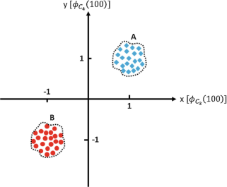
  • (i) How could you distinguish between condition A and B if you were only given ${\mathcal{V}}_{\phi }$?

  • (ii) Let us assume that ${\mathcal{V}}_{\phi }$ under conditions A and B has the same exact distribution except that for condition A the distribution is centered around the point (1,1)^T and for condition B around the point (−1,−1)^T. Let us denote this probability distribution with p(x, y) and also let us assume symmetry with respect to origin, that is, p(x, y) = p(−x, −y), and indifference to input variables’ order, i.e., p(x, y) = p(y, x). Now if we want to fit the line $y-\alpha x-\delta =0$, such that any point lying on one side of this line is designated as condition A and the other side as condition B, how should we find (α, δ)?

  • (iii) Based on your answer in (ii), find the optimal set of (α, δ), if any.

• 5. If we assume that a dipole is placed at coordinates (x, y, z), the distance between the dipole source and field space, $({x}^{\prime},{y}^{\prime},{z}^{\prime})$, is defined as $r=\sqrt{{\left(x-{x}^{\prime}\right)}^2+{\left(y-{y}^{\prime}\right)}^2+{\left(z-{z}^{\prime}\right)}^2}$.

  • (i) Calculate $\nabla \left(\frac{1}{r}\right)$, where ∇ is the gradient operator defined as $\nabla f={\left(\frac{\partial f}{\partial x},\frac{\partial f}{\partial y},\frac{\partial f}{\partial z}\right)}^{\mathrm{T}}$.

  • (ii) Calculate ${\nabla}^{\prime}\left(\frac{1}{r}\right)$, where ∇^′ is the gradient operator with respect to $({x}^{\prime},{y}^{\prime},{z}^{\prime})$, i.e., ${\nabla}^{\prime }f={\left(\frac{\partial f}{\partial {x}^{\prime }},\frac{\partial f}{\partial {y}^{\prime }},\frac{\partial f}{\partial {z}^{\prime }}\right)}^{\mathrm{T}}$.

  • (iii) Show that $\nabla \left(\frac{1}{r}\right)=-{\nabla}^{\prime}\left(\frac{1}{r}\right)$.

• 6. Assuming that a current dipole is placed at the origin of an infinitely homogeneous space pointing toward the z-direction, i.e., (x, y, z)^T = (0, 0, 0)^T and $\overline{{\mathcal{J}}^{i}}$ = (0, 0, 1)^T, using Eq. 13.3:

  • (a) Can you calculate the potential field generated by this dipole in any point $({x}^{\prime},{y}^{\prime},{z}^{\prime})$?

    Hint. $\underset{v}{\int}\nabla \left(\frac{1}{r}\right).\overline{{\mathcal{J}}^{{i}}}\left(x,y,z\right)\ dv=\nabla \left(\frac{1}{r}\right).\overline{{\mathcal{J}}^{{i}}}$, where $\overline{{\mathcal{J}}^{{i}}}$ is the current dipole moment at the origin and $\nabla \left(\frac{1}{r}\right).\overline{{\mathcal{J}}^{{i}}}$ is the inner product of the dipole moment and the gradient of the reciprocal of field point distance to dipole. This equality is due to the fact that we assumed the dipole source to be a point source at the origin. This basically is the impulse response of the Poisson’s equations, more generally referred to as the Green’s function. The inner product between vectors A = (A _x, A _y, A _z)^T and B = (B _x, B _y, B _z)^T is defined as follows: A. B = A _xB _x + A _yB _y + A _zB _z.

  • (b) Assuming that the EEG sensor is located at (0, 0, 1)^T, what number would it read as the potential (ideal conditions, noise is nonexistent)?

  • (c) What if the sensor is located at (1, 0, 0)^T?

  • (d) What if the sensor is located at (0, − 1, 0)^T?

• 7. Repeat problem 6 to calculate the magnetic field an MEG magnetometer would sense at the same locations. Use ($B=\frac{\mu }{4\pi}\int \overline{{\mathcal{J}}^{i}}\times \nabla \left(\frac{1}{r}\right) dv$) and the Green’s function hint given before. The cross product between vectors A = (A _x, A _y, A _z)^T and B = (B _x, B _y, B _z)^T is defined as follows: A × B = (A _yB _z − A _zB _y, A _zB _x − A _xB _z, A _xB _y − A _yB _x).

• 8. Based on problems 6 and 7, can you explain [and prove mathematically] why EEG signals are less sensitive to tangential sources and MEG signals to radial sources?

• 9. Let us simply assume that the lead field matrix A, of an MEG recording system with two recording channels and 3 possible sources, is given as follows:

  • (i) Assuming that the given lead field matrix models the relationship between source current density and the magnetic field in z-direction, what is the relationship between the recorded magnetic field (in z-direction) B at these sensors and the current density S = (S ₁,S ₂,S ₃)^T? Assume ideal conditions where no noise exists.

    

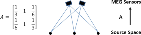
  • (ii) What would the MEG sensors record if S = (1,1,1)^T?

  • (iii) What if S = (2,−1,2)^T?

  • (iv) What if S = (3,0,3)^T?

  • (v) What if S = (1,1,1)^T + $\mathcal{t}$(2,−1,2)^T, $\left(\mathcal{t}\in \mathcal{R}\right)$?

  • (vi) Can you calculate the null space of matrix A, that is, all vectors x such that Ax = 0?

  • (vii) Can you briefly explain why the inverse problem is not unique? You can mathematically prove this using the concept of null space of a matrix.

• 10. Combining Eqs. 13.5 and 13.8:

  • (i) Can you formulate the relationship between estimated, X, and true source, S?

  • (ii) Based on the relation derived in (i), what should be the relationship between A and B, for the estimated source to be exactly the same as the true source?

  • (iii) Can linear methods, as studied in this problem, ever truly estimate the true source without any further priors or assumptions?

• 11. Can you derive Eq. 13.16 from Eq. 13.15 by differentiating Eq. 13.15 and setting it to zero?

• 12. Let us study the Bayesian approaches in more detail (Eqs. 13.20, 13.21, and 13.22). Let us assume that $\phi = Ax+{n}$ and that ${n}$ is a white Gaussian noise, ${n}\sim N\left(0,{\sigma_n}^2\right):$

  • (a) What is the probability distribution function (pdf) of ${n}$?

  • (b) What does p(ϕ| x) mean? Convince yourself that $p\left(\phi |x\right)=p(n)\propto {e}^{-\frac{1}{2{\sigma_n}^2}{\left\Vert \phi - Ax\right\Vert}^2}$.

  • (c) If we assume x ∼ N(0, σ _s ²), what is p(x)?

  • (d) Using Bayes’ rule (Eq. 13.20), formulate the posterior distribution p(x| ϕ).

  • (e) Define the likelihood of a distribution as $\mathcal{L}(x)=\ln p(x)$. Derive the posterior likelihood calculated in (iv).

  • (f) Formulate $\hat{x}=\underset{x}{\mathrm{argmax}}\mathcal{L}\left(x|\phi \right)$ and derive a similar formula to Eq. 13.15, showing that weighted minimum-norm (WMN) solutions are a form of maximum a posteriori (MAP) estimators.

• 13. The L₂-norm of a 2D vector, (x, y), is defined as $\sqrt{x^2+{y}^2},$ and the L₁-norm is defined as ∣x ∣  +  ∣ y∣. The level sets of norm functions are closed curves partitioning the space to inside and outside. On the other hand, some functions, such as lines or hyperplanes, partition the space to above and below. We will explore the level sets of these functions in simple cases and in a two-dimensional space. We will examine how these simple functions can be combined to form optimization problems, in later questions.

  • (a) Can you plot $\sqrt{x^2+{y}^2}=1$ and |x| + |y| = 1?

  • (b) Can you plot and describe the set of lines described by y + 2x = K ₀ for ${K}_0\in \mathcal{R}$? If K ₀ decreases, which direction will the line move toward? What happens when K ₀ increases?

• 14. Assuming x, y ≥ 0, how would you describe the following optimization problem?

  • (a) $\underset{x,y}{\mathrm{argmin}\ }\left(y+2x\right)$

    Subject to |x| + |y| = 1 x, y ≥ 0

    Hint. Basically, you want to minimize K ₀ (where y + 2x = K ₀) for nonnegative x, y with L₁-norm of 1.

  • (b) Can you graphically depict this optimization problem, by varying the values of K ₀?

  • (c) Based on (b), can you propose a systematic way to solve this type of an optimization problem? What are the optimal values of x ^∗, y ^∗, and K ₀ ^∗ in this problem?

• 15. Repeat problem 6 for the following optimization problem:

  $$ \underset{x,y}{\mathrm{argmin}\ }\left(y+2x\right) $$

  Subject to $\sqrt{x^2+{y}^2}=1\ x,y\ge 0$

• 16. From problems 14 and 15, can you explain why you would expect L₁-norm regularizations to induce sparsity in the solution? Sparsity in case of a 2D signal means only 1 nonzero element!

References

R. Caton, The electric currents of the brain. Br. Med. J. 2, 278 (1875)
H. Berger, Über das Elektrenkephalogramm des Menschen. Archiv f. Psychiatrie 87(1), 527–570 (1929). https://doi.org/10.1007/BF01797193
D. Cohen, Magnetoencephalography: Detection of the brain’s electrical activity with a superconducting magnetometer. Science 175(4022), 664–666 (1972). https://doi.org/10.1126/science.175.4022.664
B. He, A. Sohrabpour, E. Brown, Z. Liu, Electrophysiological source imaging: A noninvasive window to brain dynamics. Annu. Rev. Biomed. Eng. 20(1), 171–196 (2018)
B. Pesaran, M. Vinck, G.T. Einevoll, A. Sirota, P. Fries, M. Siegel, W. Truccolo, C.E. Schroder, R. Srinivasan, Investigating large-scale brain dynamics using field potential recordings: analysis and interpretation. Nat. Neurosci. 21(7), 903 (2018). https://doi.org/10.1038/s41593-018-0171-8
F.H. Lopes da Silva, EEG and MEG: Relevance to neuroscience. Neuron 80(5), 1112–1128 (2013). https://doi.org/10.1016/j.neuron.2013.10.017
M.S. Hämäläinen, R. Hari, R.J. Ilmoniemi, J. Knuutila, O.V. Lounasmaa, Magnetoencephalography—theory, instrumentation, and applications to noninvasive studies of the working human brain. Rev Mod. Phys. 65(2), 413 (1993)
J. Malmivuo, R. Plonsey, Bioelectromagnetism: Principles and Applications of Bioelectric and Biomagnetic Fields (Oxford University Press, New York, Oxford, 1995)
P.L. Nunez, R. Srinivasan, Electric Fields of the Brain: The Neurophysics of EEG (Oxford University Press, New York, 2006)
A. Sohrabpour, Y. Lu, P. Kankirawatana, J. Blount, H. Kim, B. He, Effect of EEG electrode number on epileptic source localization in pediatric patients. Clin. Neurophysiol. 126(3), 472–480 (2015)
M. Seeck, L. Koessler, T. Bast, F. Leijten, C. Michel, C. Baumgartner, B. He, S. Beniczky, The standardized EEG electrode array of the IFCN. Clin. Neurophysiol. 128, 2070 (2017)
G.A. Worrell, A.B. Gardner, S.M. Stead, S. Hu, S. Goerss, G.J. Cascino, F.B. Meyer, R. Marsh, B. Litt, High-frequency oscillations in human temporal lobe: Simultaneous microwire and clinical macroelectrode recordings. Brain 131(4), 928–937 (2008)
G. Buzsáki, F. Lopes da Silva, High frequency oscillations in the intact brain. Prog. Neurobiol. 98(3), 241–249 (2012). https://doi.org/10.1016/j.pneurobio.2012.02.004
J.D. Jirsch, E. Urrestarazu, P. LeVan, A. Olivier, F. Dubeau, J. Gotman, High-frequency oscillations during human focal seizures. Brain 129(6), 1593–1608 (2006)
Y. Lu, G.A. Worrell, H.C. Zhang, L. Yang, B. Brinkmann, C. Nelson, B. He, Noninvasive imaging of the high frequency brain activity in focal epilepsy patients. IEEE Trans. Biomed. Eng. 61(6), 1660–1667 (2014)
N. von Ellenrieder, L.P. Andrade-Valença, F. Dubeau, J. Gotman, Automatic detection of fast oscillations (40–200Hz) in scalp EEG recordings. Clin. Neurophysiol. 123(4), 670–680 (2012). https://doi.org/10.1016/j.clinph.2011.07.050
J. Jacobs, M. Zijlmans, R. Zelmann, C.E. Chatillon, J. Hall, A. Olivier, F. Dubeau, J. Gotman, High-frequency electroencephalographic oscillations correlate with outcome of epilepsy surgery. Ann. Neurol. 67(2), 209–220 (2010)
S.V. Gliske, Z.T. Irwin, C. Chestek, G.L. Hegeman, B. Brinkmann, O. Sagher, H.J.L. Garton, G.A. Worrell, W. Stacey, Variability in the location of high frequency oscillations during prolonged intracranial EEG recordings. Nat. Commun. 9(1), 2155 (2018). https://doi.org/10.1038/s41467-018-04549-2
E. Boto, N. Holmes, J. Leggett, G. Roberts, V. Shah, S.S. Meyer, L.D. Munoz, K.J. Mullinger, T.M. Tierney, S. Bestmann, G.R. Barnes, R. Bowtell, M.J. Brookes, Moving magnetoencephalography towards real-world applications with a wearable system. Nature 555(7698), 657–661 (2018). https://doi.org/10.1038/nature26147
R. Hari et al., IFCN-endorsed practical guidelines for clinical magnetoencephalography (MEG). Clin. Neurophysiol. 129(8), 1720–1747 (2018). https://doi.org/10.1016/j.clinph.2018.03.042
A. Gevins, J. Le, N.K. Martin, P. Brickett, J. Desmond, B. Reutter, High resolution EEG: 124-channel recording, spatial deblurring and MRI integration methods. Electroencephalogr. Clin. Neurophysiol. 90(5), 337–358 (1994). https://doi.org/10.1016/0013-4694(94)90050-7
P. Zhang, K. Jamison, S. Engel, B. He, S. He, Binocular rivalry requires visual attention. Neuron 71(2), 362–369 (2011)
B.M. Savers, H.A. Beagley, W.R. Henshall, The mechanism of auditory evoked EEG responses. Nature 247(5441), 481 (1974). https://doi.org/10.1038/247481a0
B. He, J. Lian, G. Li, High-resolution EEG: A new realistic geometry spline Laplacian estimation technique. Clin. Neurophysiol. 112(5), 845–852 (2001). https://doi.org/10.1016/S1388-2457(00)00546-0
A. Hillebrand, G.R. Barnes, A quantitative assessment of the sensitivity of whole-head MEG to activity in the adult human cortex. NeuroImage 16(3, Part A), 638–650 (2002). https://doi.org/10.1006/nimg.2002.1102
S. Baillet, Magnetoencephalography for brain electrophysiology and imaging. Nat. Neurosci. 20(3), 327–339 (2017)
M. Seeber, L.-M. Cantonas, M. Hoevels, T. Sesia, V. Visser-Vandewalle, C.M. Michel, Subcortical electrophysiological activity is detectable with high-density EEG source imaging. Nat. Commun. 10(1), 753 (2019). https://doi.org/10.1038/s41467-019-08725-w
F. Pizzo, N. Roehri, S.M. Villalon, A. Trebuchon, S. Chen, S. Lagarde, R. Carron, M. Gavaret, B. Giusiano, A. McGonigal, F. Bartolomei, J.M. Badier, C.G. Benar, Deep brain activities can be detected with magnetoencephalography. Nat. Commun. 10(1), 971 (2019). https://doi.org/10.1038/s41467-019-08665-5
F. Perrin, O. Bertrand, J. Pernier, Scalp current density mapping: Value and estimation from potential data. IEEE Trans. Biomed. Eng. BME-34(4), 283–288 (1987). https://doi.org/10.1109/TBME.1987.326089
B. He, R.J. Cohen, Body surface Laplacian ECG mapping. IEEE Trans. Biomed. Eng. 39(11), 1179–1191 (1992). https://doi.org/10.1109/10.168684
B. Hjorth, An on-line transformation of EEG scalp potentials into orthogonal source derivations. Electroencephalogr. Clin. Neurophysiol. 39(5), 526–530 (1975). https://doi.org/10.1016/0013-4694(75)90056-5
F. Babiloni, C. Babiloni, F. Carducci, L. Fattorini, P. Onorati, A. Urbano, Spline Laplacian estimate of EEG potentials over a realistic magnetic resonance-constructed scalp surface model. Electroencephalogr. Clin. Neurophysiol. 98(4), 363–373 (1996). https://doi.org/10.1016/0013-4694(96)00284-2
W. Besio, T. Chen, Tripolar Laplacian electrocardiogram and moment of activation isochronal mapping. Physiol. Meas. 28(5), 515–529 (2007). https://doi.org/10.1088/0967-3334/28/5/006
J.V. Haxby, A.C. Connolly, J.S. Guntupalli, Decoding neural representational spaces using multivariate pattern analysis. Annu. Rev. Neurosci. 37(1), 435–456 (2014). https://doi.org/10.1146/annurev-neuro-062012-170325
J. Linde-Domingo, M.S. Treder, C. Kerrén, M. Wimber, Evidence that neural information flow is reversed between object perception and object reconstruction from memory. Nat. Commun. 10(1), 179 (2019). https://doi.org/10.1038/s41467-018-08080-2
B. Gohel, S. Lim, M.-Y. Kim, H. Kwon, K. Kim, Dynamic pattern decoding of source-reconstructed MEG or EEG data: Perspective of multivariate pattern analysis and signal leakage. Comput. Biol. Med. 93, 106–116 (Feb. 2018). https://doi.org/10.1016/j.compbiomed.2017.12.020
R. Plonsey, Bioelectric Phenomena (Wiley Online Library, 1969). http://onlinelibrary.wiley.com/doi/10.1002/047134608X.W1403/full
B. He, T. Musha, Y. Okamoto, S. Homma, Y. Nakajima, T. Sato, Electric dipole tracing in the brain by means of the boundary element method and its accuracy. IEEE Trans. Biomed. Eng. 34(6), 406–414 (1987)
M.S. Hämäläinen, Interpreting Measured Magnetic Fields of the Brain: Estimates of Current Distributions (Helsinki University of Technology, Otaniemi, 1984)
A.M. Dale, M.I. Sereno, Improved localizadon of cortical activity by combining EEG and MEG with MRI cortical surface reconstruction: A linear approach. J. Cogn. Neurosci. 5(2), 162–176 (1993)
R.D. Pascual-Marqui, C.M. Michel, D. Lehmann, Low resolution electromagnetic tomography: A new method for localizing electrical activity in the brain. Int. J. Psychophysiol. 18(1), 49–65 (1994)
B. He, X. Zhang, J. Lian, H. Sasaki, D. Wu, V.L. Towle, Boundary element method-based cortical potential imaging of somatosensory evoked potentials using subjects’ magnetic resonance images. NeuroImage 16(3, Part A), 564–576 (2002). https://doi.org/10.1006/nimg.2002.1127
R.G. de Peralta Menendez, S.L.G. Andino, S. Morand, C.M. Michel, T. Landis, Imaging the electrical activity of the brain: ELECTRA. Hum. Brain Mapp. 9(1), 1–12 (2000)
S. Rush, D.A. Driscoll, EEG electrode sensitivity-an application of reciprocity. IEEE Trans. Biomed. Eng. BME-16(1), 15–22 (1969). https://doi.org/10.1109/TBME.1969.4502598
M.S. Hämäläinen, J. Sarvas, Realistic conductivity geometry model of the human head for interpretation of neuromagnetic data. IEEE Trans. Biomed. Eng. 36(2), 165–171 (1989)
J.C. Mosher, R.M. Leahy, P.S. Lewis, EEG and MEG: Forward solutions for inverse methods. IEEE Trans. Biomed. Eng. 46(3), 245–259 (1999)
Y. Yan, P.L. Nunez, R.T. Hart, Finite-element model of the human head: Scalp potentials due to dipole sources. Med. Biol. Eng. Comput. 29(5), 475–481 (1991)
Y. Zhang, L. Ding, W. van Drongelen, K. Hecox, D.M. Frim, B. He, A cortical potential imaging study from simultaneous extra- and intracranial electrical recordings by means of the finite element method. NeuroImage 31(4), 1513–1524 (2006). https://doi.org/10.1016/j.neuroimage.2006.02.027
C.H. Wolters, A. Anwander, X. Tricoche, D. Weinstein, M.A. Koch, R.S. MacLeod, Influence of tissue conductivity anisotropy on EEG/MEG field and return current computation in a realistic head model: A simulation and visualization study using high-resolution finite element modeling. NeuroImage 30(3), 813–826 (2006). https://doi.org/10.1016/j.neuroimage.2005.10.014
W.H. Lee, Z. Liu, B.A. Mueller, K. Lim, B. He, Influence of white matter anisotropic conductivity on EEG source localization: Comparison to fMRI in human primary visual cortex. Clin. Neurophysiol. 120(12), 2071–2081 (2009)
R.M. Gulrajani, Bioelectricity and Biomagnetism (New York, Wiley, 1998)
A.M. Dale, A.K. Liu, B.R. Fischl, R.L. Buckner, J.W. Belliveau, J.D. Lewine, E. Halgren, Dynamic statistical parametric mapping: Combining fMRI and MEG for high-resolution imaging of cortical activity. Neuron 26(1), 55–67 (2000)
Z. Liu, B. He, fMRI–EEG integrated cortical source imaging by use of time-variant spatial constraints. NeuroImage 39(3), 1198–1214 (2008)
B. He, Z. Liu, Multimodal functional neuroimaging: Integrating functional MRI and EEG/MEG. IEEE Rev. Biomed. Eng. 1, 23–40 (2008). https://doi.org/10.1109/RBME.2008.2008233
T. Musha, Y. Okamoto, Forward and inverse problems of EEG dipole localization. Crit. Rev. Biomed. Eng. 27(3–5), 189–239 (1999)
M. Scherg, D. Von Cramon, Two bilateral sources of the late AEP as identified by a spatio-temporal dipole model. Electroencephalogr. Clin. Neurophysiol./Evoked Potentials Sect. 62(1), 32–44 (1985)
H. Stefan, C. Hummel, G. Scheler, A. Genow, K. Druschky, C. Tilz, M. Kaltenhauser, R. Hopfengartner, M. Buchfelder, J. Romstock, Magnetic brain source imaging of focal epileptic activity: A synopsis of 455 cases. Brain 126(11), 2396–2405 (2003). https://doi.org/10.1093/brain/awg239
K. Kaiboriboon, S. Nagarajan, M. Mantle, H.E. Kirsch, Interictal MEG/MSI in intractable mesial temporal lobe epilepsy: Spike yield and characterization. Clin. Neurophysiol. 121(3), 325–331 (2010). https://doi.org/10.1016/j.clinph.2009.12.001
D. Cohen, B.N. Cuffin, A method for combining MEG and EEG to determine the sources. Phys. Med. Biol. 32(1), 85–89 (1987). https://doi.org/10.1088/0031-9155/32/1/013
M. Fuchs, M. Wagner, H.A. Wischmann, T. Kohler, A. Theiben, R. Drenckhahn, H. Buchner, Improving source reconstructions by combining bioelectric and biomagnetic data. Electroencephalogr. Clin. Neurophysiol. 107(2), 93–111 (1998). https://doi.org/10.1016/S0013-4694(98)00046-7
J.C. Mosher, P.S. Lewis, R.M. Leahy, Multiple dipole modeling and localization from spatio-temporal MEG data. IEEE Trans. Biomed. Eng. 39(6), 541–557 (1992)
B.D. Van Veen, W. Van Drongelen, M. Yuchtman, A. Suzuki, Localization of brain electrical activity via linearly constrained minimum variance spatial filtering. IEEE Trans. Biomed. Eng. 44(9), 867–880 (1997)
F. Babiloni, C. Babiloni, F. Carducci, L. Fattorini, C. Anello, P. Onorati, A. Urbano, High resolution EEG: A new model-dependent spatial deblurring method using a realistically-shaped MR-constructed subject’s head model. Electroencephalogr. Clin. Neurophysiol. 102(2), 69–80 (1997). https://doi.org/10.1016/S0921-884X(96)96508-X
Y. Lai, X. Zhang, W. van Drongelen, M. Kohrman, K. Hecox, Y. Ni, B. He, Noninvasive cortical imaging of epileptiform activities from interictal spikes in pediatric patients. NeuroImage 54(1), 244–252 (2011)
F. Babiloni, F. Cincotti, C. Babiloni, F. Carducci, D. Mattia, L. Astolfi, A. Basilisco, P.M. Rossini, L. Ding, Y. Ni, B. He, Estimation of the cortical functional connectivity with the multimodal integration of high-resolution EEG and fMRI data by directed transfer function. NeuroImage 24(1), 118–131 (2005)
C. Grova, J. Daunizeau, J.-M. Lina, C.G. Bénar, H. Benali, J. Gotman, Evaluation of EEG localization methods using realistic simulations of interictal spikes. NeuroImage 29(3), 734–753 (2006)
L. Ding, H. Yuan, Simultaneous EEG and MEG source reconstruction in sparse electromagnetic source imaging. Hum. Brain Mapp. 34(4), 775–795 (2013). https://doi.org/10.1002/hbm.21473
U. Mitzdorf, Current source-density method and application in cat cerebral cortex: Investigation of evoked potentials and EEG phenomena. Physiol. Rev. 65(1), 37–100 (1985). https://doi.org/10.1152/physrev.1985.65.1.37
J.-Z. Wang, S.J. Williamson, L. Kaufman, Magnetic source images determined by a lead-field analysis: The unique minimum-norm least-squares estimation. IEEE Trans. Biomed. Eng. 39(7), 665–675 (1992)
E. Biglieri, K. Yao, Some properties of singular value decomposition and their applications to digital signal processing. Signal Process. 18(3), 277–289 (1989). https://doi.org/10.1016/0165-1684(89)90039-X
Y. Shim, Z. Cho, SVD pseudoinversion image reconstruction. IEEE Trans. Acoust. Speech Signal Process. 29(4), 904–909 (1981). https://doi.org/10.1109/TASSP.1981.1163632
A.N. Tikhonov, V.Y. Arsenin, Solutions of Ill-Posed Problems (Wiley, New York, 1977)
V.A. Morozov, Methods for Solving Incorrectly Posed Problems (Springer Science & Business Media, Berlin, 1984)
P.C. Hansen, Analysis of discrete ill-posed problems by means of the L-curve. SIAM Rev. 34(4), 561–580 (1992)
P.C. Hansen, D.P. O’Leary, The use of the L-curve in the regularization of discrete ill-posed problems. SIAM J. Sci. Comput. 14(6), 1487–1503 (1993)
B. Jeffs, R. Leahy, M. Singh, An evaluation of methods for neuromagnetic image reconstruction. IEEE Trans. Biomed. Eng. BME-34(9), 713–723 (1987). https://doi.org/10.1109/TBME.1987.325996
G.H. Golub, M. Heath, G. Wahba, Generalized cross-validation as a method for choosing a good ridge parameter. Technometrics 21(2), 215–223 (1979). https://doi.org/10.1080/00401706.1979.10489751
S. Baillet, J.C. Mosher, R.M. Leahy, Electromagnetic brain mapping. IEEE Signal Process. Mag. 18(6), 14–30 (2001)
J. Daunizeau, J. Mattout, D. Clonda, B. Goulard, H. Benali, J. Lina, Bayesian spatio-temporal approach for EEG source reconstruction: Conciliating ECD and distributed models. IEEE Trans. Biomed. Eng. 53(3), 503–516 (2006). https://doi.org/10.1109/TBME.2005.869791
M. Zhu, W. Zhang, D.L. Dickens, L. Ding, Reconstructing spatially extended brain sources via enforcing multiple transform sparseness. NeuroImage 86, 280–293 (2014)
A. Sohrabpour, Y. Lu, G. Worrell, B. He, Imaging brain source extent from EEG/MEG by means of an iteratively reweighted edge sparsity minimization (IRES) strategy. NeuroImage 142, 27–42 (2016)
K. Sekihara, S.S. Nagarajan, Electromagnetic Brain Imaging: A Bayesian Perspective (Springer, Cham, 2015)
I.F. Gorodnitsky, J.S. George, B.D. Rao, Neuromagnetic source imaging with FOCUSS: A recursive weighted minimum norm algorithm. Electroencephalogr. Clin. Neurophysiol. 95(4), 231–251 (1995). https://doi.org/10.1016/0013-4694(95)00107-A
R. Pascual-Marqui, LORETA (Low Resolution Brain Electromagnetic Tomography): New authentic 3D functional Images of the brain. ISBET Newslett. Issue 5, 4–8 (1994)
L. Yang, C. Wilke, B. Brinkmann, G.A. Worrell, B. He, Dynamic imaging of ictal oscillations using non-invasive high-resolution EEG. NeuroImage 56(4), 1908–1917 (2011)
Y. Zhang, W. van Drongelen, M. Kohrman, B. He, Three-dimensional brain current source reconstruction from intra-cranial ECoG recordings. NeuroImage 42(2), 683–695 (2008). https://doi.org/10.1016/j.neuroimage.2008.04.263
V. Caune, R. Ranta, S. Le Cam, J. Hofmanis, L. Maillard, L. Koessler, V. Louis-Dorr, Evaluating dipolar source localization feasibility from intracerebral SEEG recordings. NeuroImage 98, 118–133 (2014). https://doi.org/10.1016/j.neuroimage.2014.04.058
S.A.H. Hosseini, A. Sohrabpour, B. He, Electromagnetic source imaging using simultaneous scalp EEG and intracranial EEG: An emerging tool for interacting with pathological brain networks. Clin. Neurophysiol. 129(1), 168–187 (2018)
K. Matsuura, Y. Okabe, A robust reconstruction of sparse biomagnetic sources. IEEE Trans. Biomed. Eng. 44(8), 720–726 (1997). https://doi.org/10.1109/10.605428
K. Matsuura, Y. Okabe, Selective minimum-norm solution of the biomagnetic inverse problem. IEEE Trans. Biomed. Eng. 42(6), 608–615 (1995)
K. Uutela, M.S. Hämäläinen, E. Somersalo, Visualization of magnetoencephalographic data using minimum current estimates. NeuroImage 10(2), 173–180 (1999)
M.X. Huang, A.M. Dale, T. Song, E. Halgren, D.L. Harrington, I. Podogorny, J.M. Canive, S. Lewis, R.R. Lee, Vector-based spatial–Temporal minimum L1-norm solution for MEG. NeuroImage 31(3), 1025–1037 (2006)
L. Ding, B. He, Sparse source imaging in electroencephalography with accurate field modeling. Hum. Brain Mapp. 29(9), 1053–1067 (2008)
M. Fuchs, M. Wagner, T. Köhler, H.-A. Wischmann, Linear and nonlinear current density reconstructions. J. Clin. Neurophysiol. 16(3), 267–295 (1999)
D. Wipf, S. Nagarajan, Iterative reweighted ℓ 1 and ℓ 2 methods for finding sparse solutions. IEEE J. Sel. Topics Signal Process. 4(2), 317–329 (2010)
K. Liao, M. Zhu, L. Ding, S. Valette, W. Zhang, D. Dickens, Sparse imaging of cortical electrical current densities via wavelet transforms. Phys. Med. Biol. 57(21), 6881 (2012). https://doi.org/10.1088/0031-9155/57/21/6881
K. Liao, M. Zhu, L. Ding, A new wavelet transform to sparsely represent cortical current densities for EEG/MEG inverse problems. Comput. Methods Prog. Biomed. 111(2), 376–388 (2013). https://doi.org/10.1016/j.cmpb.2013.04.015
L. Ding, Reconstructing cortical current density by exploring sparseness in the transform domain. Phys. Med. Biol. 54(9), 2683 (2009)
L. Ding, Y. Ni, J. Sweeney, B. He, Sparse cortical current density imaging in motor potentials induced by finger movement. J. Neural Eng. 8(3), 036008 (2011). https://doi.org/10.1088/1741-2560/8/3/036008
M. Zhu, W. Zhang, D.L. Dickens, J.A. King, L. Ding, Sparse MEG source imaging for reconstructing dynamic sources of interictal spikes in partial epilepsy. J. Clin. Neurophysiol. 30(4), 313–328 (2013). https://doi.org/10.1097/WNP.0b013e31829dda27
R.N. Henson, Y. Goshen-Gottstein, T. Ganel, L.J. Otten, A. Quayle, M.D. Rugg, Electrophysiological and haemodynamic correlates of face perception, recognition and priming. Cereb. Cortex 13(7), 793–805 (2003). https://doi.org/10.1093/cercor/13.7.793
D. Yao, B. He, A self-coherence enhancement algorithm and its application to enhancing three-dimensional source estimation from EEGs. Ann. Biomed. Eng. 29(11), 1019–1027 (2001)
K. Liu, Z.L. Yu, W. Wu, Z. Gu, Y. Li, S. Nagarajan, Variation sparse source imaging based on conditional mean for electromagnetic extended sources. Neurocomputing 313, 96 (2018). https://doi.org/10.1016/j.neucom.2018.06.004
A. Gramfort, D. Strohmeier, J. Haueisen, M.S. Hämäläinen, M. Kowalski, Time-frequency mixed-norm estimates: Sparse M/EEG imaging with non-stationary source activations. NeuroImage 70, 410–422 (2013)
B. He, L. Yang, C. Wilke, H. Yuan, Electrophysiological imaging of brain activity and connectivity—Challenges and opportunities. IEEE Trans. Biomed. Eng. 58(7), 1918–1931 (2011)
S. Ogawa, D.W. Tank, R. Menon, J.M. Ellermann, S.G. Kim, H. Merkle, K. Ugurbil, Intrinsic signal changes accompanying sensory stimulation: Functional brain mapping with magnetic resonance imaging. PNAS 89(13), 5951–5955 (1992)
K.K. Kwong, J.W. Belliveau, D.A. Chesler, I.E. Goldberg, R.M. Weisskoff, B.P. Poncelet, D.N. Kennedy, B.E. Hoppel, M.S. Cohen, R. Turner, Dynamic magnetic resonance imaging of human brain activity during primary sensory stimulation. PNAS 89(12), 5675–5679 (1992). https://doi.org/10.1073/pnas.89.12.5675
P.A. Bandettini, E.C. Wong, R.S. Hinks, R.S. Tikofsky, J.S. Hyde, Time course EPI of human brain function during task activation. Magn. Reson. Med. 25(2), 390–397 (1992). https://doi.org/10.1002/mrm.1910250220
S. Ogawa, T.M. Lee, A.R. Kay, D.W. Tank, Brain magnetic resonance imaging with contrast dependent on blood oxygenation. PNAS 87(24), 9868–9872 (1990)
W. Ou, A. Nummenmaa, J. Ahveninen, J.W. Belliveau, M.S. Hämäläinen, P. Golland, Multimodal functional imaging using fMRI-informed regional EEG/MEG source estimation. NeuroImage 52(1), 97–108 (2010)
J. Gotman, C. Grova, A. Bagshaw, E. Kobayashi, Y. Aghakhani, F. Dubeau, Generalized epileptic discharges show thalamocortical activation and suspension of the default state of the brain. PNAS 102(42), 15236–15240 (2005). https://doi.org/10.1073/pnas.0504935102
A. Delorme, S. Makeig, EEGLAB: An open source toolbox for analysis of single-trial EEG dynamics including independent component analysis. J. Neurosci. Methods 134(1), 9–21 (2004)
D. Brunet, M.M. Murray, C.M. Michel, Spatiotemporal analysis of multichannel EEG: CARTOOL. Comput. Intell. Neurosci. 2011, 2 (2011)
B. Fischl, FreeSurfer. NeuroImage 62(2), 774–781 (2012)
D.W. Shattuck, R.M. Leahy, BrainSuite: An automated cortical surface identification tool. Med. Image Anal. 6(2), 129–142 (2002)
D. Rivière, D. Geffroy, I. Denghien, N. Souedet, Y. Cointepas, BrainVISA: An extensible software environment for sharing multimodal neuroimaging data and processing tools. NeuroImage 47, S163 (2009)
A. Gramfort, T. Papadopoulo, E. Olivi, M. Clerc, OpenMEEG: opensource software for quasistatic bioelectromagnetics. Biomed. Eng. Online 9(1), 45 (2010)
B. He, Y. Dai, L. Astolfi, F. Babiloni, H. Yuan, L. Yang, eConnectome: A MATLAB toolbox for mapping and imaging of brain functional connectivity. J. Neurosci. Methods 195(2), 261–269 (2011)
R. Oostenveld, P. Fries, E. Maris, J.-M. Schoffelen, FieldTrip: Open source software for advanced analysis of MEG, EEG, and invasive electrophysiological data. Comput. Intell. Neurosci. 2011, 1 (2011)
A. Gramfort, M. Luessi, E. Larson, D.A. Engemann, D. Strohmeier, C. Brodbeck, L. Parkkonen, M.S. Hamalainen, MNE software for processing MEG and EEG data. NeuroImage 86, 446–460 (2014)
S.S. Dalal, J.M. Zumer, V. Agrawal, K.E. Hild, K. Sekihara, S.S. Nagarajan, NUTMEG: A neuromagnetic source reconstruction toolbox. Neurol. Clin. Neurophysiol. 2004, 52 (2004)
F. Tadel, S. Baillet, J.C. Mosher, D. Pantazis, R.M. Leahy, Brainstorm: A user-friendly application for MEG/EEG analysis. Comput. Intell. Neurosci. 2011, 8 (2011)
P.J. Magistretti, L. Pellerin, D.L. Rothman, R.G. Shulman, Energy on demand. Science 283(5401), 496–497 (1999). https://doi.org/10.1126/science.283.5401.496
P.L. Nunez, R.B. Silberstein, On the relationship of synaptic activity to macroscopic measurements: Does co-registration of EEG with fMRI make sense? Brain Topogr. 13(2), 79–96 (2000)
Acknowledgments
This work was supported in part by NIH EB021027, EB006433, NS096761, AT009263, MH114233, NSF CBET-0933067, NSF CAREER Award ECCS-0955260, NSF NRI 1208639, and NSF EPSCoR RII Track-2 1539068.
Author information
Authors and Affiliations
Corresponding author
Editor information
Editors and Affiliations