Executing Scenario-Based Specification with Dynamic Generation of Rich Events

Abstract

Scenario-Based Programming (SBP) is an approach to modeling and running complex, event-based, system behavior by composing narrower views of overall behavior. In this paper we introduce significant extensions to the strict interfaces by which scenarios in existing SBP frameworks specify what the system must, may, or must not do, and to the mechanisms that execute these scenarios: (i) we allow events with a multitude of variables and parameters; each event can become an entire model, and each event selection can be the selection of a major section of the new state of the system and the environment; (ii) we extend the basic request/block SBP interfaces with a rich set of composable constraints and functions, which can describe desired and undesired variable assignments, where each constraint may relate to all variables or to just a subset thereof; (iii) we introduce a central, application-agnostic mechanism for adding optimization to standard event selection; and (iv) we relate our method to Null-Space Behavior (NSB)—a successful compositional approach in control theory. We demonstrate these language-independent concepts through several use cases that are implemented in a variety of languages and solvers.

This paper substantially extends the paper titled “On-the-Fly Construction of Composite Events in Scenario-Based Modeling Using Constraint Solvers”, published in Modelsward 2019 [48].

1 Introduction

One of the key goals in Model Driven Engineering (MDE) is creating executable models, which, on one hand, represent how engineers and other stakeholder conceive a problem and a system, and, on the other hand, can be used directly for automatic generation of system and environment behavior: for simulation, for formal analysis, and for final production deployment. Scenario-Based Programming (SBP) [16, 40, 45] tackles this challenge by offering dynamic, run-time, composition of scenarios, each of which specifies a narrow facet of the system’s behavior, as might be described in a requirements document, resulting in cohesive integrated system behavior. Individual scenarios describe both desired behaviors, which should be manifested in the system as a whole, and undesired (or even forbidden) behaviors, which the system should avoid. The SBP principles are general, i.e., language agnostic. They have been implemented in dedicated frameworks, such as the Play-Engine and PlayGo for the visual language of Live Sequence Charts (LSC) [39, 40] and ScenarioTools [22] for the textual Scenario Modeling Language (SML). Furthermore, SBP has been implemented as libraries in programming languages like Java [41], C++ [30], and JavsScript [4], and has been amalgamated with the Statecharts visual formalism [53]. SBP has been successfully used in modeling complex systems, including industrial manufacturing, biological modeling, web-servers [30], cache coherence protocols [32], robotic controllers [25], and in new approaches for intelligent software-development assistant tools [32,33,34, 52].

In this work, we expand SBP capabilities by allowing more expressive specification of each scenario’s view of the composite behavior, and richer techniques for composing these views.

The principles of execution mechanisms used in current behavioral programming tools are as follows. System and environment behavior is modeled as a sequence of discrete events, each perhaps with one or two parameters (e.g., traffic light turns green, vehicle starts moving, vehicle makes a 45$^\circ$ right turn); all scenarios are run in parallel and are synchronized at predetermined points; at every synchronization point each scenario declares a discrete set of events it would like to see triggered, termed requested events, and a set of events it forbids from being triggered, termed blocked events; the underlying SBP infrastructure then selects for triggering a single event that is requested by at least one scenario and is not blocked by any scenarios; the selected event is then broadcast to all scenarios; scenarios can react to that event and change their declarations; and the execution continues until the next synchronization point is reached. An example appears in Fig. 1.

Fig. 1.

(From [36]) A scenario-based system for controlling the water level in a tank with hot and cold water taps. Scenarios are depicted as parallel-running transition systems that synchronize at every state. The scenario object AddHotWater repeatedly waits for WaterLow events and requests the event AddHot three times; the scenario object AddColdWater performs a symmetrical operation with cold water. In a model that includes only the objects AddHotWater and AddColdWater, the three AddHot events and three AddCold events may be triggered in any order during execution. In order to maintain the stability of the water temperature in the tank, the scenario object Stability enforces the interleaving of AddHot and AddCold events, by using event blocking. The execution trace of the resulting model appears in the event log.

Some of the benefits of SBP stem from these intuitive [19] and succinct [31] expression and composition semantics, reducing the cognitive load that might be imposed by a single composite automaton, or depicting visually the actual conditions of which events are allowed in which composite states. The approach also renders scenario-based models more amenable to automatic analysis using formal compositional techniques [21, 28, 29, 32, 37], and even makes it easier to automatically distribute, repair and synthesize such models [23, 24, 26, 35, 57, 58].

Here is how we would like to extend the current capabilities of SBP:

• 1. We wish to allow for rich events that may have multiple numeric and discrete parameters. This need is clear in the context of modern systems, such as autonomous driving, advanced robotics, and more. We believe that in this area there is a gap in most, if not all, software engineering approaches. In particular, it may well be that the recent trend to employ machine learning (ML) techniques directly to a large variety of complex problems is fueled not only by the great success of computational learning techniques in solving certain kinds of problems. It is quite accepted that for complex systems even if all rules and specifications needed for a procedural solution were available, e.g., from domain experts, or by extraction from statistical and ML tools, there are no practical engineering techniques for using these rules in building the system so that it is robust, efficient, predictable, analyzable and maintainable.

• 2. We would like to be able to view events as entire instances of object models of the system and the environment, enabling new assignments to any and all variables in a single synchronization point. As will be seen later, this concept of finding object model instance aligns well with the terminology of constraint solvers, which aim to find a model that satisfies the given constraints. These instantaneous models are not to be confused with the model of the system, which describes the objects in the system and their behaviors.

• 3. We want to extend the basic request/block SBP interfaces with a richer set of composable constraints which may relate to all variables or to just a subset thereof; further, these constraints may be organized in hierarchies or priorities of various kinds, and interfere with (or override) each other in more ways than the request/block protocol allows.

• 4. We would like to add intelligence and insight to the event (or model) selection, such that when multiple solutions satisfy the constraints, optimization techniques may be introduced, to select a preferred solution.

These extensions can be thought of as enhancing SBP’s concept of event selection to a form of event construction. We accomplish them by allowing the scenarios to present rich constraints in languages accepted by a variety of constraint solvers, and then having the SBP infrastructure invoke a solver and/or optimizer at every synchronization point to solve a composite formula, which is assembled from the declarations of all scenarios.

The work described in this paper extends our previous work [48] in several ways. First, we introduce here an extension to SBP that performs constraint resolution with optimization. Additionally, we study the concept of variable targeting in constraint specifications. We also demonstrate the applicability of our approach using additional use-cases, discuss its applicability to real-time settings, and compare the solutions it yields to related solutions proposed in the literature, particularly Null-Space behavior (NSB). Our extensions demonstrate that through the proposed enhancements to SBP, the concept of rich events can be expanded so that the entire state of the system and its environment, with its numerous variables and parameters, can be determined by behavioral decisions at every step. We propose the concept of variable targeting with proper labeling and meta processing, and implement it in Python/Z3. Finally, we introduce an implementation of the extended SBP principles, using Wolfram Mathematica.

The paper is organized as follows. In Sect. 2 we provide some necessary background on SBP and on constraint solvers. In Sect. 3 we provide the formal definitions of how SBP is to be extended to allow for the new capabilities, and in Sect. 4 we describe certain technical aspects of the implementation of SBP with various solvers. In Sect. 5 we review the main capabilities of the new approach and illustrate them with specific example applications. In Sect. 6 we review related work, and we conclude in Sect. 7.

2 Background

2.1 Scenario-Based Modeling

Formally, a scenario-based specification/model/program consists of modules termed scenarios. All scenarios run in parallel. Each scenario repeatedly declares sets of events which, from its own perspective, should, may, or must not occur at that particular point in time during the execution. The simultaneously-running scenarios are repeatedly synchronized, and a central mechanism selects events that constitute the integrated system behavior. Ideally, the scenarios do not interact with each other directly— all interactions are carried out through the common event selection and broadcasting mechanism.

Following the definitions in [41, 49], we define a scenario object O over event set E as a tuple $O = \langle Q, \delta , q_0, R, B \rangle$, where the components are interpreted as follows:

• Q is a set of states, each representing one of the predetermined synchronization points;

• $q_0$ is the initial state;

• $R:Q\rightarrow 2^E$ and $B:Q\rightarrow 2^E$ map states to the sets of events requested and blocked at these states, respectively; and

• $\delta : Q \times E \rightarrow 2^Q$ is a transition function indicating how the object reacts when an event is triggered.

Scenario objects can be composed, in the following manner. For objects $O^1 = \langle Q^1, \delta ^1, q_0^1, R^1, B^1 \rangle$ and $O^2 = \langle Q^2, \delta ^2, q_0^2, R^2, B^2 \rangle$ over a common event set E, the composite scenario object $O^1\parallel O^2$ is defined by $O^1 \parallel O^2 = \langle Q^1 \times Q^2, \delta ,\langle q_0^1,q_0^2\rangle , R^1\cup R^2, B^1\cup B^2\rangle$ where:

• $\langle \tilde{q}^1,\tilde{q}^2\rangle \in \delta (\langle q^1,q^2\rangle , e)$ if and only if $\tilde{q}^1 \in \delta ^1(q^1,e)$ and $\tilde{q}^2\in \delta ^2(q^2,e)$; and

• The union of the labeling functions is defined in the natural way; i.e., $e\in (R^1\cup R^2)(\langle q^1,q^2 \rangle )$ if and only if $e \in R^1(q^1) \cup R^2(q^2)$, and $e\in (B^1\cup B^2)(\langle q^1,q^2 \rangle )$ if and only if $e \in B^1(q^1) \cup B^2(q^2)$.

A behavioral model M is simply a collection of scenario objects $O^1, O^2,\ldots , O^n$, and the executions of M are the executions of the composite object $O = O^1\parallel O^2\parallel \ldots \parallel O^n$. Each such execution starts from the initial state of O, and in each state q along the run an enabled event is chosen for triggering, if one exists (i.e., an event $e\in R(q) - B(q)$). Then, the execution moves to state $\tilde{q}\in \delta (q,e)$, and so on.

2.2 Constraint Solvers

Broadly speaking, constraint solvers are tools that take as input a set of constraints given as a formula $\varphi$ over a set of variables V, and either (i) return a variable assignment that satisfies $\varphi$, or (ii) state that no such variable assignment exists. As mentioned above, a satisfying assignment is usually called a model, but we will try to refrain from using that term, so as to not confuse it with the model of the system under development. Different solvers differ in the kinds of constraints they allow as part of their input, and many popular solvers operate on constraints given in restricted forms of first order logic. The performance of these solvers (and the complexity of the problems they solve) also closely depends on the kinds of inputs they allow. Automated solvers have become widespread and highly successful in the last decades, particularly in tasks related to program analysis and verification [5, 14].

The types of candidate solvers relevant to our work are as follows:

Boolean Satisfiability (SAT) Solvers. These are solvers that operate on a set V of Boolean variables, and limit the constraint input $\varphi$ to be a quantifier-free propositional formula over the variables of V. The solver then attempts to find a Boolean assignment that satisfies $\varphi$. For example, for $V=\{p,q\}$, the formula $\varphi _1=(p\vee q)\wedge (p\vee \lnot q)$ is satisfiable, and one satisfying assignment is $p,\lnot q$, whereas the formula $\varphi _2=(\lnot p\vee \lnot q)\wedge p\wedge q$ is unsatisfiable. Although the Boolean satisfiability problem is NP-complete, there exist many mature tools that can solve instances that appear in practice, and which contain hundreds of thousands of variables [54]. A particular kind of SAT solver, called MaxSAT, attempts to find a Boolean assignment that satisfies as many of the input constraints as possible (and not necessarily all of them).

Linear Programming (LP) Solvers. LP solvers operate on a set V of rational variables, and the constraint formula $\varphi$ is a conjunction of linear constraints, often referred to as a linear program. For example, for the variables $V=\{x,y,z\}$, the constraint $\varphi _3=(x\le 5) \wedge (x+y\le z)$ is satisfiable, whereas the constraint $\varphi _4=(x\le 5) \wedge (y\le 2) \wedge (x+y\ge 20)$ is unsatisfiable. The general linear programming problem is known to be solvable in polynomial time, although many solvers use worst-case exponential algorithms that turn out to be more efficient in practice [13].

Satisfiability Modulo Theories (SMT) Solvers. These solvers can be regarded as generalized SAT solvers, capable of handling formulas in rich fragments of first order logic. The satisfiability of the formulas is checked subject to (i.e., modulo) background theories, which intuitively restrict the search only to satisfying assignments that “make sense” according to these certain theories. For example, considering the theory of arrays of integer elements with variable set $V=\{a,b\}$, the formula $\varphi _5=(a[3]\ge b[5])\wedge (a[4]\le b[0])$ is satisfiable, whereas the formula $\varphi _6=(a=b)\wedge (a[4]\ne b[4])$ is unsatisfiable. Modern SMT solvers support many theories of interest, including various arithmetic theories, the theory of uninterpreted functions, and theories of arrays, of sets, of strings, and others [6]. Furthermore, these background theories can be combined: for example, one can define formulas that include arrays of integers or sets of strings, etc. The SMT problem is, in general, undecidable, although certain background theories afford efficient decision procedures.

Numeric Optimization Solvers. For some optimization problems, it is beneficial to apply solvers that are guaranteed to terminate after a finite number of steps. Some tools, such as MATLAB and Mathematica, implement iterative algorithms that after a finite number of steps terminate, either converging to an optimal solution or providing an approximation thereof if one has not yet been discovered. Such solvers are useful, for example, when implementing a controller for generating real-time feedback in the context of a physical system, such as an autonomous car, a drone, a robot, etc.

The above kinds of solvers are used for many tasks in academia and industry, and all are highly successful. Many mature tools supporting them exist, and a great deal of research is being put into improving them further.

3 New Extension Mechanisms

3.1 Formal Definitions of the New Event Generation Mechanism

The mechanism underlying our extensions of SBP is as follows. At each synchronization point, instead of declaring sets of requested and blocked events, each scenario object $O_i$ can instead declare a set of constraint formulas $\varPhi =\{\varphi _i^1,\ldots ,\varphi _i^l\}$ that are intended as guiding rules for a solver-based mechanism that assembles the events. Further, these constraint formulas are labeled by a labeling function $L_i$, which maps each formula $\varphi _i^k$ into a subset of a finite set of predefined labels (or tags) $\mathcal {L}$. The labels then provide additional meta information/semantics that can guide the SBP infrastructure in assembling and composing the various formulas, such as distinguishing must constraints from may constraints, assigning different priorities to some constraints, etc.

At each synchronization point, the execution mechanism collects from all scenarios the sets of constraint formulas $\varPhi _1,\ldots ,\varPhi _n$, and assembles them into a global constraint formula $\varphi$. This formula is then passed as input to a constraint solver. If the formula is found to be satisfiable, the result (i.e., the satisfying assignment returned by the solver) is broadcast to all scenarios, which can then change their states and declarations. When no satisfying assignment is found, the system takes no action, and waits for an external event, as described in [42]. Alternatively, when the set of scenarios also includes scenarios that play the role of (i.e., simulate) the environment, no additional external events can be expected, and the system can then stop or terminate for further debugging.

Formally, we modify the definitions of SBP to support the new capabilities, via integration with constraint solvers, as follows. Let V denote a set of variables. (Note: the goal of the SBP infrastructure is to assign a value to each of these variables, at each synchronization point.) Let $\mathcal {L}$ denote a finite set of labels. We define a scenario object O over V and $\mathcal {L}$ as a tuple $O = \langle Q, \delta , q_0, C, L \rangle$, where Q is a set of states and $q_0$ is the initial state, as before. The function C (which replaces the labeling functions R and B in the original definition of SBP) maps each state $q\in Q$ to a set of constraint formulas $\varPhi =\{\varphi ^1,\ldots ,\varphi ^l\}$ over the variables of V. The function L maps each state to a labeling of these constraint formulas; i.e., $L:Q \times \xi \rightarrow 2^\mathcal {L}$, where $\xi$ represents the set of all possible formulas. By convention, we require that $L(q,\varphi )=\emptyset$ for every $\varphi$ such that $\varphi \notin C(q)$. The transition function $\delta$ is now defined as $\delta : Q\times A(V)\rightarrow 2^Q$, where A(V) is the set of all possible assignments to the variables of V. Intuitively, given a specific state q and a variable assignment $\alpha \in A(V)$ (as may be chosen by the solver-assisted execution infrastructure), invoking $\delta (q,\alpha )$ returns the set of states into which the object may transition.

In order to account for the new constraint formulas, we modify the composition operator for scenario objects, as follows: for scenario objects $O^1 = \langle Q^1, \delta ^1, q_0^1, C^1, L^1 \rangle$ and $O^2 = \langle Q^2, \delta ^2, q_0^2, C^2, L^2 \rangle$ over a common variable set V and a common label set $\mathcal {L}$, the composite scenario object $O^1\parallel O^2$ is defined by $O^1 \parallel O^2 = \langle Q^1 \times Q^2, \delta , \langle q_0^1,q_0^2\rangle , C, L\rangle$, where $\langle \tilde{q}^1,\tilde{q}^2\rangle \in \delta (\langle q^1,q^2\rangle , \alpha )$ if and only if $\tilde{q}^1 \in \delta ^1(q^1,\alpha )$ and $\tilde{q}^2\in \delta ^2(q^2,\alpha )$. The constraint-generating function C is defined as $C(\langle q^1,q^2\rangle )=C^1(q^1)\cup C^2(q^2)$; i.e., the constraints defined by the individual objects are combined and become the constraints defined by the composite object. We define $L(\langle q^1,q^2\rangle ,\varphi )= L^1(q^1,\varphi ) \cup L^2(q^2,\varphi )$, using again the convention that $L^i(q^i,\varphi ) = \emptyset$ if $\varphi \notin C^i(q^i)$.

The key difference between our extended semantics and the original is only in the event selection mechanism. As before, a behavioral model M is a collection of scenario objects $O^1, O^2,\ldots , O^n$, and the executions of M are the executions of the composite object $O = O^1\parallel O^2\parallel \ldots \parallel O^n$. Each such execution starts from the initial state of O, and after each state q along the run a variable assignment $\alpha$ is assembled, by invoking a constraint solver on a formula $\varphi$ constructed from C(q) according to the constraint labeling L. Specifically, we assume that the modeler also provides a constraint composition rule $\psi$. Given the constraint-generating function C and the labeling function L, $\psi$ interprets the labels in L and thus dictates how to construct for every state q the constraint formula $\varphi$ that should be passed along to the solver, and/or how, in general, to treat the various constraints (e.g., applying conjunctions, disjunctions and negations, applying priorities among scenarios, or applying various optimization goals when multiple solutions exist). The execution then moves to state $\tilde{q}\in \delta (q,\alpha )$, and so on.

3.2 Extension of the Request/Block Semantics of SBP

The original semantics of SBP, as defined in [41, 49], can be obtained from the new one as follows. We allow only two labels representing request constraints and block constraints respectively. In addition, we define the variable set V to contain precisely one variable e, representing the triggered event. Next, we syntactically restrict the constraint formulas $\varphi _i$ to be of the form $e=c$ for some constant c; and finally, for any state q we define the constraint composition rule to be:

(1)

Intuitively, at each state, each scenario object can declare events it requests (expressed as constraints tagged with the label “Request”), and those it wants to block (expressed as constraints tagged with the label “Block”). The constraint composition rule then translates these individual constraints into a global formula representing the fact that the triggered event needs to be requested and not blocked; i.e., it should satisfy the conjunction of being requested with the negation of being blocked.

When using these particular restrictions, the straightforward solver of choice is a SAT solver: since the formula $\varphi$ only contains propositional connectives and the variable e can only take on a finite number of values, we can encode these possible values using a finite set of Boolean variables (this process is often called bit-blasting). A modern SAT solver can then be used for selecting the triggered event very quickly, in a way that is likely to enable an execution that is sufficiently fast for many application domains.

Beyond just SAT solvers, we propose in this paper to use SMT solvers. This allows for richer constraint languages that employ theories such as the theory of real numbers. Further, we do not restrict V to contain only a single variable. This enables the constraint resolutions to yield not only the choice of a value or event from a set of candidates, but an assignment of values to an entire system configuration.

As explained in more detail in Sect. 5.6, to make sure that all variables are properly assigned, and to comply with the scenario’s intentions of which variable should constrain the values of each other variable, we enrich the “Request” tagging and labeling with a subset S of the set V of variable names, i.e., we use the labels . The following formula extends formula (1), in stating that for each variable in V there must be at least one constraint satisfied in the constraint resolution, which stated that it wishes that this variable be set.

(2)

4 Implementation Infrastructure

To demonstrate and evaluate our approach, we developed proof-of-concept applications on multiple platforms.

The first implementation uses MATLAB/Simulink. Scenario objects generate their constraints as strings containing textual descriptions of the constraints. These strings are then passed into MATLAB’s equation and system solver, which is called solve. The solution yielded by the solver is then translated into variable values that flow along the classical Simulink connectors as input to other blocks, driving standard Simulink behavior. The results of this behavior (i.e., the effect on the environment) are also fed back into the scenarios, which can then change the constraints they present. See Sect. 5.7 for more details on this case study.

In a second, experimental implementation, described in Sect. 5.8, we used solvers and optimizers of Wolfram’s Mathematica to create composite behavior from SBP-like specifications.

A third implementation, used in the code examples in this paper, is based on the Python language and the Z3 SMT solver [17]. We use Python and Z3 to implement the event selection formula (2). To simplify the specifications, we also added the label Wait-For that allows a scenario to maintain its declaration as long as the condition tagged by this label is not met. The default for this tag, if not present, is True, i.e., if a scenario does not specify an explicit “Wait-For” condition, its request and block statements are valid for the next event only. Note that since formulas that are labeled only with “Wait-For” do dot appear in Eq. (2) they do not affect event construction, only the progress of the scenarios.

In our implementation, each scenario object is coded as a Python generator. A generator is a function that can pause itself and pass control back to its caller at any point, using the yield idiom. It can then be subsequently resumed when it is re-invoked with the language’s next idiom. The infrastructure mimics the parallel execution, as follows (the core of the execution mechanism code for a similar system appears in [48]). It calls each generator sequentially, waiting for it to yield control, and then calls the next one. When all scenarios reach their respective synchronization points, the infrastructure collects the constraints passed by the scenarios (in the form of a Python dictionary containing Z3 constraints labeled by keys from the set {Request (S), Block, and Wait-For}). It then invokes the solver to obtain an assignment for all variables of V that satisfies Eq. (2). We also support the label Request (without the set S) that is automatically translated to the label Request (S), where S is the set of all the variables that appear in the labeled formula.

5 Modeling with the New Composition Principles

What can be achieved by using this new composition mechanism? How does it help system engineers and modelers? We review these capabilities via several illustrative examples:

• 1. An extension of the water-tank example with hot and cold water taps.

• 2. A UAV/drone that is capable of maneuvers in three dimensional space.

• 3. A software installation management system and/or software product line management system, where dependencies and conflicts among software libraries/features/packages determine which component is to be installed or included in a particular delivery.

• 4. Solving the Towers of Hanoi puzzle. In this application the scenarios describe the (a) essence of the puzzle, i.e., the initial state (all disks on one peg), the goal (all disks are on some other peg), and rules (e.g., disks on a peg must be ordered by decreasing diameter); and (b) behavioral scenarios for executing an iterative solution.

• 5. Navigating a flock/swarm of robots, in two-dimensional space, towards a destination, while bypassing obstacles. The goal is to move all robots towards a configuration where the set’s centroid (“center of gravity”) is at a pre-specified destination, while the individual robots avoid colliding with the obstacles, whose boundaries were also pre-specified.

Listings of actual scenarios for these applications/models are available as part of the supplementary material [15].

5.1 Constructing Rich Multi-variable Events

We now illustrate the richness of the events that can be modeled our extension.

In the drone example, the UAV is capable of simultaneous vertical and horizontal maneuvers. We can define V to include two variables, $V=\{v,h\}$, where v represents the vertical angular velocity and h the horizontal angular velocity. One scenario can set upper and lower bounds on the vertical angular velocity, say due to the drone’s mechanical limitations, and another can limit the horizontal angular velocity (see Fig. 2). Here we require no labeling of the constraints, i.e. $\mathcal {L}=\emptyset$, and the constraint composition rule $\psi$ is a simply a conjunction of all the individual constraints.

Fig. 2.

Two scenario objects, represented as transition systems (state machines) that, respectively, put hard limits on the vertical and horizontal angular velocities of the drone. Each scenario has a single synchronization point, as indicated by its single state, in which it contributes a constraint (e.g., $\varphi _1= -5\le v\le 5$) to the global constraint set. The only transition, a self loop that does not depend on the variable assignment returned by the solver, indicates that the scenario continues to contribute this constraint, regardless of the satisfying assignment discovered by the solver.

Without any additional limitations, i.e., if only these two scenarios existed in the system, the constraint formula at any synchronization point would be

$$\varphi ~~=~~\varphi _1\wedge \varphi _2~~=~~(-5\le v\le 5)\wedge (-10\le h\le 10)$$

Because the constraints are arithmetical, linear constraints, we can use an LP solver to dispatch them; and indeed, in this case an LP solver will return an assignment such as $v=3, h=0$. Other scenario objects in the system, referred to as actuator scenarios, may then receive and process these values, and through appropriate APIs adjust the drone’s engines accordingly.

Let us now extend the example with a particular flight situation, where another scenario navigates the drone to its destination, and that scenario is requesting a right turn at an angular velocity of at least 6 degrees per second:

$$\varphi _3 = h\ge 6$$

We also add an obstacle-detection scenario that detected the presence of a cellular-communication antenna tower up ahead, and which, in order to circumvent the obstacle, is requesting that the elevation be increased or that a left turn be initiated:

$$\varphi _4= h \le -3 \vee v \ge 2$$

When the solver is given the global constraint formula $\varphi =\wedge _{i=1}^4\varphi _i$, it can construct the composite event by yielding the solution $h=8,v=3$, which satisfies all constraints by both turning right and increasing the drone’s altitude.

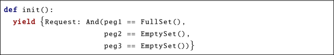
In the Towers of Hanoi example (see detailed scenarios in Sect. 5.5 and in the supplementary material), we observe how the scenarios form a complete configuration; i.e., they specify which disc should reside on which peg, and which pegs would be designated as source and destination respectively. Thus, in each step, the SBP execution mechanism implicitly constructs the entire three-peg configuration. The instructions for the actual moving of a disk from one peg to another, is (purposely for this example) only implicit, in contrast to more standard programming where this step would be at the core of the program.

5.2 Rich Constraint Specifications

While the events and the environment configurations are greatly enriched by supporting the assignment of many variables in every step, one should note that feeding the solvers with arbitrary expressions allows scenarios to introduce constraints that in themselves are rich. For example, a scenario can introduce an irregularly-shaped obstacle by describing the curve of its boundary in a single expression. Or, the effect of gradually changing speeds and friction coefficients as a car slows down or swerves on an uneven road, can be introduced as a single rich function of time and location.

5.3 Enhanced Incrementality

Figure 3 lists the Python code for the water tank system, depicted as a set of transition systems in Fig. 1. During execution, the satisfying assignments obtained by the solver alternate between assigning to true and to false, and vice versa.

Fig. 3.

A solver-based SBP specification for the water-tank application. The (resp., ) variables/flags indicate that a dose of hot (resp., cold) water is to be added to the tank. The rules/requirements are: (1) do not add hot and cold doses at the same time; (2) add three doses of hot water; (3) add three doses of cold water; (4) never add two doses of the same type consecutively.

Fig. 4.

New requirements for the water tap model: (1) the temperature of a hot event must be above 50; (2) the temperature of a cold event must be below 50; (3) the temperature of an event that follows a hot event must be above 20; (4) the temperature of an event that follows a cold event must be below 80.

Consider now a customer-driven requirements change. E.g., the requirement prohibiting two consecutive doses of the same type is removed, and the customer decides to add requirements about water temperature, as presented in Fig. 4 and its caption. In an SBP model, one can simply add and remove the respective lines of scenario code. These additional requirements introduce a new solver variable . The new scenarios can control this new variable, and the solver can handle it, in addition to preexisting variables, without changing other scenarios. Note that the remaining scenarios are unaware of the new variable.

5.4 Rich Constraint-Composition Semantics

So far, we have seen two examples for constraint composition rules (annotated as $\psi$ above): request-and-block and conjunction. We now demonstrate another composition rule.

In a system for managing software package dependencies, package A may require package B and/or it may be incompatible with package C, and thus cannot be installed alongside C. The state of the entire system is the set of currently installed software packages. Finally, the system is given a user-supplied goal, such as install Package A, and is then required to install A and any prerequisite packages, while removing the smallest number of packages currently installed with which A and its dependencies are incompatible.

To model this, we can utilize a MaxSAT solver, whose input formula consists of subformulas labeled either hard or soft. The solver finds an assignment that satisfies the hard constraints and as many of the soft constraints as possible. For each package dependency, we will specify a scenario that adds a hard constraint representing this dependency, and we will model the currently-installed packages as soft constraints that are introduced by designated scenarios. The MaxSAT solver will thus return an assignment such that the goal package and its prerequisites are installed while the number of previously installed packages that are removed is minimized [2, 51].

More specifically, the variable set V consists of a Boolean variable for each software package, e.g. $\{x_A,x_B,x_C,\ldots \}$, which are true if and only if the package is installed. Actuator scenarios respond to changes in variable values by installing or removing a package. Our label set is $\{h,s\}$, indicating whether a constraint is hard or soft, respectively. Each dependency is represented by a dedicated object; for example, the requirement “A requires B” is encoded by the top scenario object in Fig. 5. Other objects are used for encoding the soft constraints representing the currently installed packages; an example appears in the bottom scenario object in Fig. 5.

The composition rule $\psi$ constructs the formula $\varphi$ (to be passed to the MaxSAT solver) as the conjunction of the individual scenario objects’ constraints, and marks these constraints as hard or soft according to their labels.

Fig. 5.

Software-package Management Example: (Left) A scenario object that specifies that installing A requires B and labels the constraint as hard for the MaxSAT solver. (Right) A scenario that adds $x_B$ as a soft constraint if package B is currently installed (left state), and contributes no constraints if it is not installed (right state). Switching between the states is performed according to the assignment discovered by the solver; specifically, it depends on whether $x_B$ is assigned to true or not. We assume the package is initially installed.

5.5 Combining “Stories” with Constraints

An important feature of SBP is the ability of each scenario object to describe an aspect of system behavior as a “story”; i.e., a scenario of events in time. This description does not mandate, as in standard programming, a complete step-by-step prescription of all process steps.

We illustrate this concept via the Towers of Hanoi example. Our SBP model for solving the puzzle is based on the following iterative (rather than recursive) algorithm:

Repeat the following two steps: (1) move the smallest disk to the “next” peg to the right (cyclically, or modulo three); and then (2) move “any” disk that is not the smallest (there is only one option for this).

Using the Python/Z3 implementation of SBP, the (rich) events, or system states can be modeled using the following state variables:

The variables and are used to model the next action to be taken.

Note that the variables , , and , which represent the disks on the three pegs, are sets. Recomputing them at every step further illustrates the richness of events and event selection, as discussed in Sect. 5.1. Furthermore, observe that in this particular model we use sets rather than ordered entities such as arrays or lists. We can do so for two independent reasons: (a) the particular system is for executing a solution, and not for solving the puzzle, and as in other models, not all assumptions must be explicitly coded; (b) in the representation of the problem in the SMT solver the “identity” of a disk is also its size and its location in the linear order (much as a collection of two-dimensional vectors $\langle x,y \rangle$ can imply relative locations for multiple pairs of points in a 2D space without explicitly stating this fact).

The main scenario that provides the core steps of the algorithm states that the variables and should be chosen so that, repeatedly, (1) disk zero is moved one peg to the right (cyclically), and (2) disk zero is not moved:

This ability to use SBP to extract and highlight the core steps of an algorithm into separate scenarios, distinguishing them from technicalities like initialization, termination, data management and other mandatory bookkeeping, is discussed in greater detail in the proposal for Scenario-Based Algorithmics [44].

We model the rest of the behavior of the solution with the following scenarios:

• The values of variables and must always be different from each other and in the range 1,2,3 (notice the use of the blocking idiom):

  

  This scenario is coded to never resume and change states; its constraints always hold, though the same behavior could be exhibited with a specification that contains a loop that resumes after any event ( ) and then returns to the same state.

• The initial state of the pegs is $\langle \{0,\dots ,n\},\emptyset ,\emptyset \rangle$:

  

• The smallest disk on the source peg must be smaller than the smallest disk on the destination peg:

  

• The source peg must not be empty:

  

• The smallest disk from the peg should move to peg:

  

5.6 Specifying Targeted Constraints

Using the constraint solvers allows each scenario to relate to some variables, while ignoring others. This is another source of expressive power. However, since the solver must, at every step, assign values to each of the variables, it is the modeler’s responsibility to specify for each variable at least one scenario that requests a value for it. While this is normally not a significant burden, there are some fine points that must be handled, and for which we offer a particular interface.

Consider the situation in Fig. 6, where two scenarios deal with separate variables, $x_1$ and $x_2$, respectively. The first scenario requests that $x_1$ be greater than 50, and the second requests that $x_2$ be greater than 50. In traditional SBP, if each of these two scenarios were to request, say, the coordinates for a robot’s destination, exactly (and only) one of the two requests would be satisfied, but both scenarios would be able to react to the choice (e.g., abandon requests that were not chosen, or maintain the request until it is satisfied, perhaps after visiting the destination that was chosen first). However, the current case is different. Since the first scenario is not aware of the second one, the designer implicitly assumes that the only may constraint for $x_1$ is that it be greater than 50, hence it does not expect the solver to allow an assignment to $x_1$ that is smaller than 50. According to our semantics, however, the composition rules produces the constraint $\psi =x_1>50 \vee x_2>50$, which is satisfied, e.g., by the assignment $\{x_1= 0, x_2 = 51\}$. A way to avoid this unintended behavior is to label each proposition with the variable that it is aware of and to solve for each set of variables separately. Another way to avoid the problem is to look for assignments that maximize the number of satisfied may constraints, e.g., by using solvers that optimize the number of satisfied clauses.

Fig. 6.

Unintended behavior with the Request semantics when using Equation (1). Solving $(x_1 {<}50) \vee (x_2{>}50)$, the assignment $\{x_1=0, x_2=51\}$ is valid, despite the fact that no scenario specified that $x_1$ may be smaller than 50.

In another case that must be handled, recall that, when specifying a constraint like $x=y$, a modeler may have different intents: whether the values for both x and y are to be chosen, or the value for x should be chosen such that it is equal to the value of y that was determined by other means, or the value for y should be implied by that of the predetermined value of x. The need to distinguish between these intents is particularly important in our setting, where the constraint solver may be asked to set (almost) all variables of the system and its environment, and may thus yield surprising results, such as having a vehicle avoid an obstacle by moving the obstacle. Using existing idioms to specify environment assumptions, like “the coordinates of this obstacle cannot change” is not enough, because the intent to change or not change a particular variable may vary from one scenario to another, or from one scenario state to another, even within the same scenario.

In our implementation, we address this by using the labeling system. E.g., specifying in the algorithm “story” scenario, and in the disk-moving actuator scenario, we indicate that the first request is to assign values only to and to and the second request is to assign values only to , , and .

The event selection mechanism is then changed to not only satisfy one request while obeying all blocking statements, but to satisfy at least one request for changing each of the variables for which there exists a request.

Thus, removing the and the from the above labels would allow for assignments that are consistent with one of the two requests but are not consistent with the other one (since in SBP not all requests must be satisfied).

The labeling of which variables can be set by a particular constraint is optional. When absent, the default is that the request applies to all, and only, the variables mentioned in the request.

This feature can be seen to provide additional expressive power, as follows. The formal definition and the implementation allow the additional tagging of the requests to include labels that are not necessarily variable names, or are variable names but ones that are not mentioned in the particular mathematical formulation of the constraint at hand. Thus, a scenario can specify that its requested constraints may be ignored altogether if other constraints labeled in the same way are satisfied.

5.7 Real-Time Reactivity

Even though solvers are designed to apply complex mathematical and logical operations and extensive searches, they can be also be used in real-time reactive systems that need to provide fine-grained discretization of near-continuous behavior.

To illustrate this, consider a model for a controlled follower rover that needs to track a leader rover while keeping a safe distance from it. The follower must accommodate nearly-arbitrary leader behavior, constrained only by basic, reasonable bounds on the leader’s speed and turn angles. This served as a challenge problem in the MDETOOLS’18 workshop, where the organizers supplied a simulator for driving the participants’ demonstrations. (See mdetools.github.io/mdetools18/challengeproblem.html.)

The simulator periodically emits the locations of the rovers, the distance between them, and the heading angle of the follower. The follower advancement and turning is controlled by setting the power for the left and right wheels.

The scenarios’ code is shown in Fig. 7: (i) : the bounds for the pR and pL variables, indicating the power to the right and left wheels; (ii) : forward and backward motion in reaction to relative distance; i.e., when the rovers are too far apart or too close the follower accelerates, decelerates or even reverses its direction; (iii) : steering towards the leader by turning the wheels when the relative angle (based on the latest simulator input) exceeds a specified value ($3^{\circ }$), the follower turns left or right towards the leader; (iv) : calculating the needed wheel power(s) for an already-triggered turn.

This example demonstrates the ability to construct complex behavior at run time, using distinct, modular, behavioral aspects.

The resulting system behavior is indeed very similar to the one presented in [20], which resulted from using SBP without a constraint solver, employing direct request-and-block logic, and which could request only finite sets of events. The use of constraint-solvers enabled, e.g., the scenario, to specify infinitely many options and allows, as demonstrated by the scenario, to further decompose the specification and to better align with the requirements.

Fig. 7.

Main scenarios of the leader-follower rover model (see explanation in the text).

The real-time capabilities of this solver-based composition is further demonstrated in the Patrol Vehicle example (described here only briefly, in order to fit space constraints), this time in a MATLAB/Simulink framework, using MATLAB solvers. This is a simulation of an autonomous vehicle that moves repeatedly in a fixed route in the shape of the figure eight, and is subject to strict speed demands and constraints, as reflected by the following scenarios: (1) always attempt to accelerate to a maximum pre-specified speed; (2) when arriving at a sharp curve, reduce speed below a specified value until exiting the curve; and (3) after driving at a speed that is higher than a certain value for longer than a certain time limit, reduce the allowed speed and acceleration to be below some other limits, for a certain amount of time (e.g., to avoid overheating or wearing out of the motor).

In addition to the real-time perspective, this example also illustrates the ability to model “stories” (see Sect. 5.5) that progress from one state to another and present different constraints at different times and states. Thus, for example, specifying the speed constraints that hold only after detecting the arrival at (or departure from) a sharp curve, or after the passage of a certain amount of time, appears quite intuitive and well aligned with the stated requirements. This can be contrasted with the less intuitive use of ever-present constraints, each constantly requiring a conjunction of conditions, e.g., current-speed-and-current-road-curvature, or, current-speed-and-time-since-certain-past-event.

5.8 Event Construction with Optimization

In this section, we show how the computational tools (namely, solvers) can also be applied to enrich the event construction with optimization of event-selection and variable assignment choices. This optimization capability is a step towards being able to manage multiple concurrent prioritized goals. This part of the work is inspired by the Null Space Behaviour (NSB) technique [1] in control theory, where composition and optimization of controllers is based on linear matrix operations, and where computing solutions for lower priority goals is done within the null space of the matrices used for the achieving higher priority goals.

This richer example also further illustrates other key properties discussed earlier. These include the ability to construct decisions with a multitude of variables; the ability to compose scenarios, each of which has a partial view of the system behavior; and, more importantly, the ability to specify what can or cannot be changed in the system and its environment.

The system in this example coordinates and guides the motion of a flock of robots (a.k.a. a multi-robot) in a two-dimensional space, as proposed in [1]. Both our approach and NSB are based on first designing simple controllers for achieving individual aspects of the required behaviour, and then composing them into a combined controller, whose emergent behaviour addresses all the requirements together.

The requirements for the flock’s motion are: (i) the centroid (“center of gravity”) of the flock should move in the direction of a specified point; (ii) a robot may not travel faster than 10 meters per second; (iii) initially, the robots are placed at equal distances on (the perimeter/curve of) a given circle; (iv) while moving, the robots should strive to maintain the circle formation; (v) the robots should stay within a specified rectangular region; (vi) the robots should not path through a specified elliptical obstacle; (vii) the centroid should also not pass through the given elliptical obstacle; (viii) the robots should maintain a minimal specified distance between any two.

In this implementation, the solver we used is the “FindMinimum” procedure from Wolfram’s Mathematica.

We formalized each requirement as an objective function or a blocking constraint to be presented to the solver. Specifically, we created a separate module/formula for each requirement. This modeling approach helps engineers and other stakeholders examine how the behaviour of a system might change when individual requirements are added, removed, or changed.

The solver was used to steer the multi-robot iteratively, in a greedy approach. Conceptually, at each step, all possible movements of the flock were considered and an optimal one was chosen. The resulting motions of each step were used to move the robots’ coordinates, and this information then served as the input for forming the equations for the next step. In future enhancements additional parameters can be considered in subsequent steps, such as past speeds and directions, in the interest of creating smoother motion or detecting situations where a robot is stuck in a tight corner.

The simulation ran successfully at about 20 steps per second (i.e., at intervals of 50 ms), thus supporting the claim that solvers can be used for real-time control systems. Clearly, faster processors now enable the running of new and complex computational tools for applications that previously demanded solutions to focus on leanness and efficiency (as in the case of NSB).

The use of the Mathematica solver enables composing the controllers in a way that manages goals hierarchically. One approach is to nest the calls for finding optimal solutions, and pass the results of each invocation as a constraint on the search for the next-lower goal in the hierarchy ladder. This can be done as follows:

$$ \mathop {\mathrm {arg\,max}} \{ f_2(x,v) :v \in \mathop {\mathrm {arg\,max}} \{ f_1(x,v) :v \in \mathbb {R}^{2n}\}\} $$

Here, n is the number of robots, $x \in \mathbb {R}^{2n}$ is a vector representing the positions of the robots in the plane, $v\in \mathbb {R}^{2n}$ is a vector representing the horizontal and vertical velocities that the controller needs to assign to the robots, and $f_1$ and $f_2$ represent the higher-priority and lower-priority goal functions, such as reaching the target destination, avoiding an obstacle, or preserving a formation.

The idea in this formulation is to only create sets of commands that are optimal with respect to the high-priority function, while using the low-priority function as a secondary consideration within the first solution space (similarly to sorting database records by a primary and secondary sort keys).

Other composition rules can support more refined controller combinations; e.g., composing the constraints in parallel to achieve a joint objective function, and controlling goal priorities via weights as opposed to solving for one goal and only then for the other.

The general characteristics of the solution’s emergent behaviour is similar to the behaviours shown in the NSB paper [1]. In particular, casual observation makes it clear that in both cases global solutions are handled with narrower local views; i.e., the scenario-weaving mechanism returns the control commands only for a specific time instance. A detailed comparison of the two approaches according to criteria like solution quality (e.g., successful termination, path length and smoothness of trajectory and speed), computational cost/efficiency, the ability to provide formal correctness proofs, and ease of development, is beyond the scope of the current paper.

The demonstration of SBP with Mathematica is still in early stages. We have not built interfaces between a procedural/scripting language like Java or Python to Mathematica. Hence, the present example does not (yet) demonstrate the SBP capabilities of scenarios that follow a “story”, changing states and declaration following the occurrence of relevant events. Given that SBP principles are language agnostic, and our experience with developing such interfaces in multiple languages and environments, we regard this issue is a technicality.

Other interesting challenges we encountered include the following. First, there were several technical issues to be addressed. For example, the solver was not able to cope with rectangular and other non-elliptical obstacles. Clearly, this should not be attributed to the use of SBP, and we expect that engineers will be able to specify constraints and objective functions that indeed test the limits of each solver’s capabilities.

A second issue is that, as stated earlier, the solver is applied locally, in very short time intervals, and without look-ahead or backward planning. This can cause some robots to get stuck in tight corners, not recognizing that they have to reverse some distance in order to get back on track. Finding a composition technique that allows for global solutions, e.g., for adding a requirement that the path be the shortest possible, or that it meet some other overall conditions, remains as future research. Note that global solutions do not mandate look-ahead that is provided by the execution infrastructure. As in NSB, the individual scenarios can contain the needed logic. For example, the flock may apply the “right hand rule” a localized approach to finding paths in certain mazes; or pilot/scout robots can explore the perimeter of the obstacle, reporting to others, who then plan a trajectory with straightforward geometry. Specialized sensors (simulating ordinary long-distance vision, or the availability of maps) can detect obstacles from a distance, triggering bypass trajectories that are less likely to get stuck in narrow crevasses. Alternatively, recovery scenarios can exercise “simulated annealing”, detecting when robots are stuck and driving them to return and explore new directions.

Another important issue is verification, and especially, compositional verification. The basic-style SBP lent itself very well to compositional verification, which helps tackle the state explosion that often hinders application of formal methods to complex reactive systems [29]. How does one specify the assumptions and guarantees of scenarios when their declarations include complex assertions that are understood only by rich solvers? A first step could be to use yet another kind of solver for composing behaviors, one that is geared especially for such a verification purpose [18].

6 Related Work

In this paper, we propose a particular approach to run-time composition of behavior, namely, extending the composition rules of existing SBP-style frameworks with specification and solving of constraints. We now briefly compare SBP to other mechanisms for execution-time composition of events, with a special focus on the present context of constraint specifications (an earlier, related analysis appears in [45]).

An important feature of SBP is its intuitiveness and succinctness. These properties are a consequence of the ability to specify forbidden behavior directly and explicitly, rather than doing so using control-flow conditions, designed to prevent certain pieces of code or specification from actually doing the undesired action. In SBP, this feature was originally embodied in the use of concrete lists of requested events and filter-based blocking. Using this paper’s extensions, this is done with constraint solvers. For example, one can now build and test the specification that a vehicle is not allowed to enter a road intersection when the traffic light is red, even before having coded how vehicles behave. Other approaches, such as business-workflow engines, simulation engines, and tools for test-driven development, often support intuitive specification of executable use cases and scenarios, but their support for generic composition of multiple allowed scenarios and forbidden scenarios is limited. Conventional object oriented and procedural programming, logic programming and functional programming languages provide for composition of behaviors, but the requirements’ use cases and scenarios are not directly visible in the code. Instead, they are typically reflected only in emergent properties of the actual execution.

The principles of SBP have been implemented in several languages, in both centralized and distributed environments. These implementations have positioned SBP as a design pattern for using constructs like messaging, semaphores and threads, and concepts such as agent-orientation for achieving incrementality and alignment of code with a set of requirements.

Publish-subscribe is a related framework for parallel composition, which does not provide language support for forbidden behavior. Aspect oriented programming [50] supports specifying and executing cross-cutting program instructions on top of a base application, but, unlike SBP, it does not allow for specifying forbidden behavior, state management within an aspect, or symmetry between aspects and base code.

Other behavior-based models, such as Brooks’s subsumption architecture [12], Branicky’s behavioral programming [11], and LEGO Mindstorms leJOS (see [3]), call for constructing systems from behaviors. The SBP formalism is language-independent, has multiple implementations, and extends in a variety of ways each of the coordination and arbitration mechanisms used by those architectures.

The execution semantics employed by SBP is similar to the event-based scheduling of SystemC [46], which uses cyclical co-routine scheduling by synchronization, evaluation, update and notification. SBP is different from SystemC in that it offers support for specifying scenarios and forbidden scenarios that directly correspond with the original requirements, while SystemC provides a particular framework for composing parallel components in certain designs and architectures. In SBP, synchronization is an inherent technique for continuously complying with the constraints posed by the requirements, whereas in SystemC synchronization is used for the coordination of an otherwise parallel component execution. This also implies differences in the semantic details of synchronization, queuing, event selection, and state management within each parallel component.

The BIP language (behavior, interaction, priority) [8] utilizes the concept of glue for assembling components. It pursues goals similar to SBP’s, with a focus on correct-by-construction systems. SBP is more geared towards the execution of intuitively specified behaviors and constraints, and the run-time resolution of these constraints.

As mentioned earlier, SBP has recently been implemented using the visual formalism of Statecharts. The Yakindu Statecharts tool now offers an extension of Statecharts’ original support for concurrent, orthogonal and hierarchical state machines [27] with the optional specification of requested and blocked events in any state, accompanied by an enhanced event selection semantics [53]. These enhancements provide the formal definitions of SBP principles, which are based on transition systems and state machines (see, e.g., [41]), with a direct, concrete executable implementation that is readily understood by humans. This allows to directly cast inter-object behaviour, which typically modelled with Statecharts and other state-based languages, in the same formalism and language as intra-object behaviour.

In SBP, the direct execution and/or simulation of a model is termed play-out. Play-out is achieved by considering all constraints of the various scenarios before each event selection. Thus, the computational burden required for each runtime decision depends mainly on the number of scenarios, and does not depend on the number of states in each scenario or on the nondeterministic branching in future system and environment behavior. In contrast, many general program synthesis approaches for reactive systems (see, e.g., [9]) apply planning, model-checking, and other techniques to resolve environment assumptions and specification constraints a-priori. This gives rise to a strategy (e.g., a deterministic finite automaton) for successfully handling all possible environment behaviors that may be encountered in all reachable program states. Synthesis has been applied to SBP specifications with the request-and-block idioms in, e.g., [43].

General synthesis techniques typically have to deal with very large state graphs. Often, this is done via run-time planning (also termed online/on-the-fly synthesis) (see, e.g., [10]). In this approach, an execution mechanism considers a single starting state of the system and its environment, thus limiting the number of system and/or environment actions considered in the search. Such a technique was implemented in SBP in, e.g., smart play-out [38]. An intriguing future research avenue is to perform run-time look-ahead, or complete program synthesis during development, for SBP specifications with rich constraint specifications like the ones discussed in this paper. Such research could include identifying categories of constraint specifications that are richer than the filters and lists used in traditional SBP, but which are still more amenable to synthesis than arbitrary constraints.

Our proposed use of constraint solvers to directly control the execution of SBP specifications differs from other uses of these tools in the verification and analysis of systems, including symbolic execution [55], bounded model-checking [7], concolic testing [56], and others. SMT solvers have previously been applied in performing such analysis tasks also in the context of SBP; e.g., by extending SMT solvers to deal more efficiently with transition systems [47] and by using the solvers to efficiently prove compositional properties for collections of SBP scenarios [29].

7 Conclusion

We have described a substantial extension of the Scenario-Based programming design and modeling approach for complex systems. By enabling the invocation of general, rich, and well-proven solvers and optimizers at every decision that the system makes, we enable modelers to perform sophisticated, yet trusted, composition of modular requirement specifications. At the same time, each narrow requirement can itself be as deep and rich as the domain professional that presented it wishes it to be. The enhancements allow scenario objects to interact with each other in far more subtle and intricate ways than is possible with only the original request-and-block idioms. All these capabilities enable engineers to use SBP in order to more directly create faithful models of complex systems. The theoretical principles of this extension are demonstrated through numerous applications that explore the capabilities, and limits, of the approach.

Future research directions include making intelligent run-time decisions using look-ahead (with model checking facilities), development-time and run-time program synthesis, and applying machine learning techniques for improving program decisions over time. These tools exist already in basic forms for traditional SBP, and have been shown to be useful. However, extending them to the present formulation will entail accounting for the more flexible event selection process.

References

Antonelli, G., Arrichiello, F., Chiaverini, S.: The NSB control: a behavior-based approach for multi-robot systems. Paladyn, J. Behav. Robot. 1(1), 48–56 (2010)
Argelich, J., Lynce, I.: CNF instances from the software package installation problem. In: Proceedings of 15th RCRA Workshop on Experimental Evaluation of Algorithms for Solving Problems with Combinatorial Explosion (2008)
Arkin, R.C.: Behavior-Based Robotics. MIT Press, Cambridge (1998)
Bar-Sinai, M., Weiss, G., Shmuel, R.: BPjs: an extensible, open infrastructure for behavioral programming research. In: Proceedings of 21st ACM/IEEE International Conference on Model Driven Engineering Languages and Systems (MODELS), pp. 59–60 (2018)
Barrett, C., Kroening, D., Melham, T.: Problem Solving for the 21st Century: Efficient Solvers for Satisfiability Modulo Theories. London Mathematical Society and Smith Institute for Industrial Mathematics and System Engineering (2014)
Barrett, C., Tinelli, C.: Satisfiability modulo theories. In: Clarke, E., Henzinger, T., Veith, H., Bloem, R. (eds.) Handbook of Model Checking, pp. 305–343. Springer, Cham (2018). https://doi.org/10.1007/978-3-319-10575-8_11
Biere, A., Cimatti, A., Clarke, E., Zhu, Y.: Symbolic model checking without BDDs. In: Cleaveland, W.R. (ed.) TACAS 1999. LNCS, vol. 1579, pp. 193–207. Springer, Heidelberg (1999). https://doi.org/10.1007/3-540-49059-0_14
Bliudze, S., Sifakis, J.: A notion of glue expressiveness for component-based systems. In: van Breugel, F., Chechik, M. (eds.) CONCUR 2008. LNCS, vol. 5201, pp. 508–522. Springer, Heidelberg (2008). https://doi.org/10.1007/978-3-540-85361-9_39
Bloem, R., Jobstmann, B., Piterman, N., Pnueli, A., Saar, Y.: Synthesis of reactive(1) designs. J. Comput. Syst. Sci. 78(3), 911–938 (2012)
Blum, A.L., Furst, M.L.: Fast planning through planning graph analysis. Artif. Intell. 90(1–2), 281–300 (1997)
Branicky, M.: Behavioral Programming. In: Working Notes AAAI Spring Symposium on Hybrid Systems and AI (1999)
Brooks, R.: A robust layered control system for a mobile robot. Robot. Autom. 2(1), 14–23 (1986)
Chvátal, V.: Linear Programming. Freeman W.H., New York (1983)
Clarke, E., Henzinger, T., Veith, H., Bloem, R.: Handbook of Model Checking. Springer, Heidelberg (2018). https://doi.org/10.1007/978-3-319-10575-8
Harel, D., Katz, G., Marron, A., Sadon, A., Weiss, G.: Supplementary Material for Scenario-based Programming with Rich Event Construction (2019). http://www.b-prog.org/ccismw19
Damm, W., Harel, D.: LSCs: breathing life into message sequence charts. J. Formal Methods Syst. Des. (FMSD) 19(1), 45–80 (2001)
de Moura, L., Bjørner, N.: Z3: an efficient SMT solver. In: Ramakrishnan, C.R., Rehof, J. (eds.) TACAS 2008. LNCS, vol. 4963, pp. 337–340. Springer, Heidelberg (2008). https://doi.org/10.1007/978-3-540-78800-3_24
Frehse, G., et al.: SpaceEx: scalable verification of hybrid systems. In: Gopalakrishnan, G., Qadeer, S. (eds.) CAV 2011. LNCS, vol. 6806, pp. 379–395. Springer, Heidelberg (2011). https://doi.org/10.1007/978-3-642-22110-1_30
Gordon, M., Marron, A., Meerbaum-Salant, O.: Spaghetti for the main course?: observations on the naturalness of scenario-based programming. In: Innovation and Technology in Computer Science Education, ITiCSE 2012. ACM (2012). https://doi.org/10.1145/2325296.2325346
Greenyer, J., Bar-Sinai, M., Weiss, G., Sadon, A., Marron, A.: Modeling and programming a leader-follower challenge problem with scenario-based tools. In: Proceedings of 21st ACM/IEEE International Conference on Model Driven Engineering Languages and Systems (MODELS), pp. 376–385 (2018)
Greenyer, J., Gritzner, D.: Generating correct, compact, and efficient PLC Code from scenario-based GR(1) specifications. In: System-Integrated Intelligence: Challenges for Product and Production Engineering (SYSINT) (2018)
Greenyer, J., et al.: ScenarioTools—a tool suite for the scenario-based modeling and analysis of reactive systems. J. Sci. Comput. Program. 149, 15–27 (2017)
Greenyer, J., Gritzner, D., Katz, G., Marron, A.: Scenario-based modeling and synthesis for reactive systems with dynamic system structure in scenariotools. In: Proceedings of 19th ACM/IEEE International Conference on Model Driven Engineering Languages and Systems (MODELS), pp. 16–23 (2016)
Greenyer, J., et al.: Distributed execution of scenario-based specifications of structurally dynamic cyber-physical systems. In: International Conference on System-Integrated Intelligence: Challenges for Product and Production Engineering (SYSINT), pp. 552–559 (2016)
Gritzner, D., Greenyer, J.: Synthesizing executable PLC code for robots from scenario-based GR(1) specifications. In: Seidl, M., Zschaler, S. (eds.) STAF 2017. LNCS, vol. 10748, pp. 247–262. Springer, Cham (2018). https://doi.org/10.1007/978-3-319-74730-9_23
Harel, D. Kantor, A., Katz, G., Marron, A., Weiss, G., Wiener, G.: Towards behavioral programming in distributed architectures. J. Sci. Comput. Program. (J. SCP) 98, 233–267 (2015)
Harel, D.: Statecharts: a visual formalism for complex systems. J. Sci. Comput. Program. (J. SCP) 8(3), 231–274 (1987)
Harel, D., Kantor, A., Katz, G.: Relaxing synchronization constraints in behavioral programs. In: McMillan, K., Middeldorp, A., Voronkov, A. (eds.) LPAR 2013. LNCS, vol. 8312, pp. 355–372. Springer, Heidelberg (2013). https://doi.org/10.1007/978-3-642-45221-5_25
Harel, D., Kantor, A., Katz, G., Marron, A., Mizrahi, L., Weiss, G.: On composing and proving the correctness of reactive behavior. In: Proceedings of 13th International Conference on Embedded Software (EMSOFT), pp. 1–10 (2013)
Harel, D., Katz, G.: Scaling-up behavioral programming: steps from basic principles to application architectures. In: International Workshop on Programming Based on Actors, Agents, and Decentralized Control (AGERE!), pp. 95–108 (2014)
Harel, D., Katz, G., Lampert, R., Marron, A., Weiss, G.: On the succinctness of idioms for concurrent programming. In: Proceedings of 26th International Conference on Concurrency Theory (CONCUR), pp. 85–99 (2015)
Harel, D., Katz, G., Marelly, R., Marron, A.: An initial wise development environment for behavioral models. In: Proceedings of 4th International Conference on Model-Driven Engineering and Software Development (MODELSWARD), pp. 600–612 (2016)
Harel, D., Katz, G., Marelly, R., Marron, A.: First steps towards a wise development environment for behavioral models. Int. J. Inf. Syst. Model. Des. (IJISMD) 7(3), 1–22 (2016)
Harel, D., Katz, G., Marelly, R., Marron, A.: Wise computing: toward endowing system development with proactive wisdom. IEEE Comput. 51(2), 14–26 (2018)
Harel, D., Katz, G., Marron, A., Weiss, G.: Non-intrusive repair of reactive programs. In: Proceedings of 17th IEEE International Conference on Engineering of Complex Computer Systems (ICECCS), pp. 3–12 (2012)
Harel, D., Katz, G., Marron, A., Weiss, G.: Non-intrusive repair of safety and liveness violations in reactive programs. Trans. Comput. Collect. Intell. (TCCI) 16, 1–33 (2014)
Harel, D., Katz, G., Marron, A., Weiss, G.: The effect of concurrent programming idioms on verification: a position paper. In: Proceedings of 3rd International Conference on Model-Driven Engineering and Software Development (MODELSWARD), pp. 363–369 (2015)
Harel, D., Kugler, H., Marelly, R., Pnueli, A.: Smart play-out of behavioral requirements. In: Aagaard, M.D., O’Leary, J.W. (eds.) FMCAD 2002. LNCS, vol. 2517, pp. 378–398. Springer, Heidelberg (2002). https://doi.org/10.1007/3-540-36126-X_23
Harel, D., Maoz, S., Szekely, S., Barkan, D.: PlayGo: towards a comprehensive tool for scenario based programming. In: Proceedings of 10th International Conference on Automated Software Engineering (ASE), pp. 359–360 (2010)
Harel, D., Marelly, R.: Come, Let’s Play: Scenario-Based Programming Using LSCs and the Play-Engine. Springer, Heidelberg (2003). https://doi.org/10.1007/978-3-642-19029-2
Harel, D., Marron, A., Weiss, G.: Programming coordinated behavior in Java. In: D’Hondt, T. (ed.) ECOOP 2010. LNCS, vol. 6183, pp. 250–274. Springer, Heidelberg (2010). https://doi.org/10.1007/978-3-642-14107-2_12
Harel, D., Marron, A., Weiss, G., Wiener, G.: Behavioral programming, decentralized control, and multiple time scales. In: Proceedings of 1st SPLASH Workshop on Programming Systems, Languages, and Applications Based on Agents, Actors, and Decentralized Control (AGERE!), pp. 171–182 (2011)
Harel, D., Segall, I.: Synthesis from live sequence chart specifications. Comput. Syst. Sci. 78(3), 970–980 (2012)
Harel, D., Marron, A.: Toward scenario-based algorithmics. In: Böckenhauer, H.-J., Komm, D., Unger, W. (eds.) Adventures Between Lower Bounds and Higher Altitudes. LNCS, vol. 11011, pp. 549–567. Springer, Cham (2018). https://doi.org/10.1007/978-3-319-98355-4_32
Harel, D., Marron, A., Weiss, G.: Behavioral programming. Commun. ACM 55(7), 90–100 (2012)
IEEE: Standard SystemC Lang. Ref. Manual. IEEE (2006)
Katz, G., Barrett, C., Harel, D.: Theory-aided model checking of concurrent transition systems. In: Proceedings of 15th International Conference on Formal Methods in Computer-Aided Design (FMCAD), pp. 81–88 (2015)
Katz, G., Marron, A., Sadon, A., Weiss, G.: On-the-fly construction of composite events in scenario-based modeling using constraint solvers. In: Model-Driven Engineering and Software Development, MODELSWARD 2019, pp. 141–154 (2019). https://doi.org/10.5220/0007573801410154
Katz, G.: On module-based abstraction and repair of behavioral programs. In: Proceedings of 19th International Conference on Logic for Programming, Artificial Intelligence and Reasoning (LPAR), pp. 518–535 (2013)
Kiczales, G., et al.: Aspect-oriented programming. In: Aksit, M., Matsuoka, S. (eds.) ECOOP 1997. LNCS, vol. 1241, pp. 220–242. Springer, Heidelberg (1997). https://doi.org/10.1007/BFb0053381
Mancinelli, F., Boender, J., Di Cosmo, R., Vouillon, J., Durak, B., Leroy, R.: Treinen: managing the complexity of large free and open source package based software distributions. In: Proceedings of 21st IEEE/ACM International Conference on Automated Software Engineering (ASE), pp. 199–208 (2006)
Marron, A., et al.: Six (im)possible things before breakfast: building-blocks and design-principles for wise computing. In: Proceedings of 19th ACM/IEEE International Conference on Model Driven Engineering Languages and Systems (MODELS), pp. 94–100 (2016)
Marron, A., Hacohen, Y., Harel, D., Mülder, A., Terfloth, A.: Embedding scenario-based modeling in statecharts. In: Proceedings of 5th International Workshop on Model-Driven Robot Software Engineering (MORSE) (2018)
Nadel, A.: Understanding and improving a modern SAT solver, Ph.D. thesis, Tel Aviv University (2009)
Păsăreanu, C., Visser, W.: A survey of new trends in symbolic execution for software testing and analysis. Int. J. Softw. Tools Technol. Transf. 11(4), 339–353 (2009)
Sen, K.: Concolic testing. In: Proceedings of 22nd IEEE/ACM International Conference on Automated Software Engineering (ASE), pp. 571–572 (2007)
Steinberg, S., Greenyer, J., Gritzner, D., Harel, D., Katz, G., Marron, A.: Distributing scenario-based models: a replicate-and-project approach. In: Proceedings of 5th International Conference on Model-Driven Engineering and Software Development (MODELSWARD), pp. 182–195 (2015)
Steinberg, S., Greenyer, J., Gritzner, D., Harel, D., Katz, G., Marron, A.: Efficient distributed execution of multi-component scenario-based models. Commun. Comput. Inf. Sci. (CCIS) 880, 449–483 (2018)
Author information
Authors and Affiliations
Corresponding author
Editor information
Editors and Affiliations
Rights and permissions
Copyright information
© 2020 Springer Nature Switzerland AG
About this paper
Cite this paper
Harel, D., Katz, G., Marron, A., Sadon, A., Weiss, G. (2020). Executing Scenario-Based Specification with Dynamic Generation of Rich Events. In: Hammoudi, S., Pires, L., Selić, B. (eds) Model-Driven Engineering and Software Development. MODELSWARD 2019. Communications in Computer and Information Science, vol 1161. Springer, Cham. https://doi.org/10.1007/978-3-030-37873-8_11
Download citation
DOI: https://doi.org/10.1007/978-3-030-37873-8_11
Published:
Publisher Name: Springer, Cham
Print ISBN: 978-3-030-37872-1
Online ISBN: 978-3-030-37873-8
eBook Packages: Computer ScienceComputer Science (R0)