Non-Committing Encryption with Quasi-Optimal Ciphertext-Rate Based on the DDH Problem

Abstract

Non-committing encryption (NCE) was introduced by Canetti et al. (STOC ’96). Informally, an encryption scheme is non-committing if it can generate a dummy ciphertext that is indistinguishable from a real one. The dummy ciphertext can be opened to any message later by producing a secret key and an encryption random coin which “explain” the ciphertext as an encryption of the message. Canetti et al. showed that NCE is a central tool to achieve multi-party computation protocols secure in the adaptive setting. An important measure of the efficiently of NCE is the ciphertext rate, that is the ciphertext length divided by the message length, and previous works studying NCE have focused on constructing NCE schemes with better ciphertext rates.

We propose an NCE scheme satisfying the ciphertext rate based on the decisional Diffie-Hellman (DDH) problem, where is the security parameter. The proposed construction achieves the best ciphertext rate among existing constructions proposed in the plain model, that is, the model without using common reference strings. Previously to our work, an NCE scheme with the best ciphertext rate based on the DDH problem was the one proposed by Choi et al. (ASIACRYPT ’09) that has ciphertext rate . Our construction of NCE is similar in spirit to that of the recent construction of the trapdoor function proposed by Garg and Hajiabadi (CRYPTO ’18).

1 Introduction

1.1 Background

Secure multi-party computation (MPC) allows a set of parties to compute a function of their inputs while maintaining the privacy of each party’s input. Depending on when corrupted parties are determined, two types of adversarial settings called static and adaptive have been considered for MPC. In the static setting, an adversary is required to declare which parties it corrupts before the protocol starts. On the other hand, in the adaptive setting, an adversary can choose which parties to corrupt on the fly, and thus the corruption pattern can depend on the messages exchanged during the protocol. Security guarantee in the adaptive setting is more desirable than that in the static setting since the former naturally captures adversarial behaviors in the real world while the latter is somewhat artificial.

In this work, we study non-committing encryption (NCE) which is introduced by Canetti, Feige, Goldreich, and Naor [4] and known as a central tool to achieve MPC protocols secure in the adaptive setting. NCE is an encryption scheme that has a special property called non-committing property. Informally, an encryption scheme is said to be non-committing if it can generate a dummy ciphertext that is indistinguishable from real ones, but can later be opened to any message by producing a secret key and an encryption random coin that “explain” the ciphertext as an encryption of the message. Cannetti et al. [4] showed how to create adaptively secure MPC protocols by instantiating the private channels in a statically secure MPC protocol with NCE.

Previous Constructions of NCE and their Ciphertext Rate. The ability to open a dummy ciphertext to any message is generally achieved at the price of efficiency. This is in contrast to ordinary public-key encryption for which we can easily obtain schemes the size of whose ciphertext is by using hybrid encryption methodology, where n is the length of an encrypted message and is the security parameter. The first NCE scheme proposed by Canetti et al. [4] only needs the optimal number of rounds (that is, two rounds), but it has ciphertexts of -bits for every bit of an encrypted message. In other words, the ciphertext rate of their scheme is , which is far from that of ordinary public-key encryption schemes. Subsequent works have focused on building NCE schemes with better efficiency.

Beaver [1] proposed a three-round NCE scheme with the ciphertext rate based on the decisional Diffie-Hellman (DDH) problem. Damgård and Nielsen [8] generalized Beaver’s scheme and achieved a three-round NCE scheme with ciphertext rate based on a primitive called simulatable PKE which in turn can be based on concrete problems such as the DDH, computational Diffie-Hellman (CDH), and learning with errors (LWE) problems. Choi, Dachman-Soled, Malkin, and Wee [7] further improved these results and constructed a two-round NCE scheme with ciphertext rate based on a weaker variant of simulatable PKE called trapdoor simulatable PKE which can be constructed the factoring problem.

The first NCE scheme achieving a sub-linear ciphertext rate was proposed by Hemenway, Ostrovsky, and Rosen [20]. Their scheme needs only two rounds and achieves the ciphertext rate $\mathcal {O}\left( \log n \right)$ based on the $\phi$-hiding problem which is related to (and generally believed to be easier than) the RSA problem, where n is the length of messages. Subsequently, Hemenway, Ostrovsky, Richelson, and Rosen [19] proposed a two-round NCE scheme with the ciphertext rate based on the LWE problem. Canetti, Poburinnaya, and Raykova [5] showed that by using indistinguishability obfuscation, an NCE scheme with the asymptotically optimal ciphertext rate (that is, $1+o(1)$) can be constructed. Their scheme needs only two rounds but was proposed in the common reference string model.

Despite the many previous efforts, as far as we know, we have only a single NCE scheme satisfying a sub-linear ciphertext rate based on widely and classically used problems, that is, the scheme proposed by Hemenway et al. [19] based on the LWE problem. Since NCE is an important cryptographic tool in constructing MPC protocols secure in the adaptive setting, it is desirable to have more constructions of NCE satisfying a better ciphertext rate.

1.2 Our Contribution

We propose an NCE scheme satisfying the ciphertext rate based on the DDH problem. The proposed construction achieves the best ciphertext rate among existing constructions proposed in the plain model, that is, the model without using common reference strings. The proposed construction needs only two rounds, which is the optimal number of rounds for NCE. Previously to our work, an NCE scheme with the best ciphertext rate based on the DDH problem was the one proposed by Choi et al. [7] that satisfies the ciphertext rate . We summarize previous results on NCE and our result in Table 1.

We first show an NCE scheme that we call basic construction, which satisfies the ciphertext rate . Then, we give our full construction satisfying the ciphertext rate by extending the basic construction using error-correcting codes. Especially, in the full construction, we use a linear-rate error-correcting code which can correct errors of weight up to a certain constant proportion of the codeword length.

Table 1. Comparison of existing NCE schemes. The security parameter is denoted by, and the message length n. Common-domain TDP can be instantiated based on the CDH and RSA problems. Simulatable and trapdoor simulatable PKE can be instantiated based on many computational problems realizing ordinary PKE. $^{(*)}$ This scheme uses common reference strings.

Our construction of NCE utilizes a variant of chameleon encryption. Chameleon encryption was originally introduced by Döttling and Garg [10] as an intermediate tool for constructing an identity-based encryption scheme based on the CDH problem. Roughly speaking, chameleon encryption is public-key encryption in which we can use a hash value of a chameleon hash function and its pre-image as a public key and a secret key, respectively. We show a variant of chameleon encryption satisfying oblivious samplability can be used to construct an NCE scheme with a sub-linear ciphertext rate. Informally, oblivious samplability of chameleon encryption requires that a scheme can generate a dummy hash key obliviously to the corresponding trapdoor, and sample a dummy ciphertext that is indistinguishable from a real one, without using any randomness except the dummy ciphertext itself.

Need for the DDH Assumption. A key and a ciphertext of the CDH based chameleon encryption proposed by Döttling and Garg [10] together form multiple Diffie-Hellman tuples. Thus, it seems difficult to sample them obliviously unless we prove that the knowledge of exponent assumption [2, 18] is false. In order to solve this issue, we rely on the DDH assumption instead of the CDH assumption. Under the DDH assumption, a hash key and a ciphertext of our chameleon encryption are indistinguishable from independent random group elements, and thus we can perform oblivious sampling of them by sampling random group elements directly from the underlying group.

Public Key Size. As noted above, we first give the basic construction satisfying the ciphertext rate , and then extend it to the full construction satisfying the ciphertext rate . In addition to satisfying only the ciphertext rate , the basic construction also has a drawback that its public key size depends on the length of a message quadratically.

A public key of the basic construction contains ciphertexts of our obliviously samplable chameleon encryption. The size of those ciphertexts is quadratic in the length of an input to the associated chameleon hash function similarly to the construction by Döttling and Garg [10]. Since the input length of the chameleon hash function is linear in the message length of the basic construction, the public key size of the basic construction depends on the message length quadratically.

Fortunately, we can remove this quadratic dependence by a simple block-wise encryption technique. Thus, in the full construction, we utilize such a block-wise encryption technique in addition to the error-correcting code. By doing so, we reduce not only the ciphertext rate to , but also the public key size to linear in the length of a message as in the previous constructions of NCE.

Relation with Trapdoor Function by Garg and Hajiabadi [14]. There has been a line of remarkable results shown by using variants of chameleon encryption, starting from the one by Cho, Döttling, Garg, Gupta, Miao, and Polychroniadou [6]. This includes results on identity-based encryption [3, 9,10,11], secure MPC [6, 16], adaptive garbling schemes [15, 17], and so on. Garg and Hajiabadi [14] showed how to realize trapdoor function (TDF) based on the CDH problem using a variant of chameleon encryption called one-way function with encryption.¹

Our construction of NCE can be seen as an extension of that of TDF by Garg and Hajiabadi. Our formulation of chameleon encryption is based on that of one-way function with encryption. Concretely, we define chameleon encryption so that it has recyclability introduced by Garg and Hajiabadi as a key property in their work.

1.3 Paper Organization

Hereafter, in Sect. 2, we first review the definition of NCE. Then, in Sect. 3, we provide high-level ideas behind our construction of NCE. In Sect. 4, we formally define and construct obliviously samplable chameleon encryption. In Sect. 5, using obliviously samplable chameleon encryption, we construct an NCE scheme that we call the basic construction satisfying the ciphertext rate . Finally, in Sect. 6, we improve the basic construction and provide the full construction that achieves the ciphertext rate .

2 Preliminaries

Let PPT denote probabilistic polynomial time. In this paper, always denotes the security parameter. For a finite set X, we denote the uniform sampling of x from X by $x\overset{\$}{\leftarrow }X$. $y{\leftarrow }\mathsf {A}(x;r)$ denotes that given an input x, a PPT algorithm $\mathsf {A}$ runs with internal randomness r, and outputs y. A function f is said to be negligible if , and we write to denote that f is negligible. Let denotes the Hamming weight of . $\mathbb {E}\left[ X \right]$ denotes expected value of X. [n] denotes $\left\{ 1,\dots ,n \right\}$.

Lemma 1 (Chernoff bound)

For a binomial random variable X. If $\mathbb {E}\left[ X \right] \le \mu$, then for all $\delta >0$, $\Pr \left[ X\ge (1+\delta )\mu ) \right] \le e^{-\frac{\delta ^2}{2+\delta }\mu }$ holds.

We provide the definition of the DDH assumption and its variants used in the proof of Theorem 1. We first introduce the leftover hash lemma.

Lemma 2 (Leftover hash lemma)

Let X and Y are sets. Let $\mathcal {H}:=\{\mathsf {H}:X\rightarrow Y\}$ be a universal hash family. Then, the distributions $(\mathsf {H}, \mathsf {H}(x))$ and $(\mathsf {H}, y)$ are $\sqrt{\frac{\left|Y\right|}{4\left|X\right|}}$-close, where $\mathsf {H}\overset{\$}{\leftarrow }\mathcal {H}$, $x\overset{\$}{\leftarrow }X$, and $y\overset{\$}{\leftarrow }Y$.

We review some computational assumptions. Below, we let $\mathbb {G}$ be a cyclic group of order $p$ with a generator $g$. We also define the function $\mathsf {dh}\left( \cdot ,\cdot \right)$ as $\mathsf {dh}\left( g^a,g^b \right) \,{:=}\,g^{ab}$ for every $a,b\in \mathbb {Z}_p$. We start with the decisional Diffie-Hellman (DDH) assumption.

Definition 1 (Decisional Diffie-Hellman Assumption)

We say that the DDH assumption holds if for any PPT adversary $\mathcal {A}$,

holds, where .

We introduce a lemma that is useful for the proof of oblivious samplability of our chameleon encryption. We can prove this lemma by using the self reducibility of the DDH problem.

Lemma 3

Let n be a polynomial of $\lambda$. Let $g_{i,b}\overset{\$}{\leftarrow }\mathbb {G}$ for every $i\in [n]$ and $b\in \{0,1\}$. We set $M:=(g_{i,b})_{i\in [n],b\in \{0,1\}}\in \mathbb {G}^{2\times n}$.

Then, if the DDH assumption holds, for any PPT adversary $\mathcal {A}$, we have

where $M^\rho =(g_{i,b}^\rho )_{i\in [n],b\in \{0,1\}}\in \mathbb {G}^{2\times n}$ and $R\leftarrow \mathbb {G}^{2\times n}$.

We next define the hashed DDH assumption which is a variant of the DDH assumption.

Definition 2 (Hashed DDH Assumption)

Let $\mathcal {H}=\{\mathsf {H_{\mathbb {G}}}:\mathbb {G}\rightarrow \{0,1\}^\ell \}$ be a family of hash functions. We say that the hashed DDH assumption holds with respect to $\mathcal {H}$ if for any PPT adversary $\mathcal {A}$,

holds, where , , and .

In this work, we use the hashed DDH assumption with respect to a hash family $\mathcal {H}$ whose output length $\ell$ is small enough such as or . In this case, by using a family of universal hash functions $\mathcal {H}$, we can reduce the hardness of the hashed DDH problem to that of the DDH problem by relying on the leftover hash lemma. Formally, we have the following lemma.

Lemma 4

Let $\mathcal {H}=\{\mathsf {H_{\mathbb {G}}}:\mathbb {G}\rightarrow \{0,1\}^\ell \}$ be a family of universal hash functions, where . Then, if the DDH assumption holds, the hashed DDH assumption with respect to $\mathcal {H}$ also holds by the leftover hash lemma.

Non-Committing Encryption. A non-committing encryption (NCE) scheme is a public-key encryption scheme that has efficient simulator algorithms satisfying the following properties. The simulator can generate a simulated public key $pk$ and a simulated ciphertext $CT$. Later can explain the ciphertext as encryption of any plaintext. Concretely, given a plaintext can output a pair of random coins for key generation and encryption , as if $pk$ was generated by the key generation algorithm with the random coin , and $CT$ is encryption of with the random coin .

Some previous works proposed NCE schemes that are three-round protocols. In this work, we focus on NCE that needs only two rounds, which is also called non-committing public-key encryption, and we use the term NCE to indicate it unless stated otherwise. Below, we introduce the definition of NCE according to Hemenway et al. [19].

Definition 3 (Non-Committing Encryption)

A non-committing encryption scheme $\mathtt {NCE}$ consists of the following PPT algorithms .

• : Given the security parameter , using a random coin , it outputs a public key and a secret key .

• : Given a public key and a plaintext , using a random coin , it outputs a ciphertext .

• : Given a secret key and a ciphertext , it outputs or $\bot$.

• : Given the security parameter , it outputs a simulated public key $pk$, a simulated ciphertext $CT$, and an internal state .

• : Given a plaintext and a state , it outputs random coins for key generation and encryption .

We require $\mathtt {NCE}$ to satisfy the following correctness and security.

• Correctness. $\mathtt {NCE}$ is called $\gamma$-correct, if for any plaintext ,

  

  When , we call it correct. Note that $\gamma$ cannot be equal to 1 in the plain model (i.e., the model without using common reference strings).

• Security. For any stateful PPT adversary $\mathcal {A}$, we define two experiments as follows.

  

  We say that $\mathtt {NCE}$ is secure if

  

  holds for every PPT adversary $\mathcal {A}$.

3 Ideas of Our Construction

In this section, we provide high-level ideas behind our construction of NCE.

As a starting point, we review the three-round NCE protocol proposed by Beaver [1], which contains a fundamental idea to build NCE from the DDH problem. Next, we show how to extend it and construct a two-round NCE scheme whose ciphertext rate is . Then, we show how to reduce the ciphertext rate to , and obtain our main result. Finally, we state that our resulting construction can be described by using a variant of chameleon encryption, and it can be seen as an extension of trapdoor function proposed by Garg and Hajiabadi [14].

3.1 Starting Point: Beaver’s Protocol

Beaver’s NCE protocol essentiality executes two Diffie-Hellman key exchange protocols in parallel. This protocol can send a 1-bit message. The ciphertext rate is . We describe the protocol below and in Fig. 1.

• Step1. Let $\mathbb {G}$ be a group of order p with a generator g. The sender picks a random bit and an exponent , and then sets . The sender also generates a random group element obliviously, i.e., without knowing the discrete log of . The sender sends to the receiver and stores the secret . The random coin used in this step is .

• Step2. The receiver picks a random bit and an exponent , and then sets . The receiver also obliviously generates . Moreover, the receiver computes and obliviously samples . The receiver sends to the sender. The random coin used in this step is .

• Step3. The sender checks whether holds or not, by checking if holds. With overwhelming probability, this equation holds if and only if . If , the sender sends , and otherwise quits the protocol.

• Step4. The receiver recovers the message by .

Fig. 1.

The description of Beaver’s protocol [1].

We next describe the simulator for this protocol.

• Simulator. The simulator simulates a transcript , and as follows. It generates and sets

  

  The simulator also generates .

  The simulator can later open this transcript to both messages 0 and 1. In other words, for both messages, the simulator can generate consistent sender and receiver random coins. For example, when opening it to , the simulator sets , and outputs and as the sender’s and receiver’s opened random coins, respectively.

• Security. Under the DDH assumption on $\mathbb {G}$, we can prove that any PPT adversary $\mathcal {A}$ cannot distinguish the pair of transcript and opened random coins generated in the real protocol from that generated by the simulator. The only difference of them is that is generated as a random group element in the real protocol, but it is generated as in the simulation. When the real protocol proceeds to Step. 4, we have with overwhelming probability. Then, the random coins used by the sender and receiver (and thus given to $\mathcal {A}$) does not contain exponents of and , that is, and . Thus, under the DDH assumption, $\mathcal {A}$ cannot distinguish randomly generated from . Thus, this protocol is a secure NCE protocol.

This protocol succeeds in transmitting a message only when , and otherwise it fails. Note that even when , the protocol can transmit a message because in Step. 3, the sender knows the receiver’s secret . However, in that case, we cannot construct a successful simulator. In order to argue the security based on the DDH assumption, we have to ensure that either one pair of exponents or is not known to the adversary, but when , we cannot ensure this.

Next, we show how to extend this protocol into a (two-round) NCE scheme and obtain an NCE scheme with the ciphertext rate .

3.2 Extension to Two-Round NCE Scheme

As a first attempt, we consider an NCE scheme $\mathtt {NCE}_{\mathtt {lin}}^1$ that is a natural extension of Beaver’s three-round NCE protocol. Intuitively, $\mathtt {NCE}_{\mathtt {lin}}^1$ is Beaver’s protocol in which the role of the sender and receiver is reversed, and the sender sends a message even when and are different. Specifically, the receiver generates the public key and secret key , and the sender generates the ciphertext , where , and are generated in the same way as those in Beaver’s protocol. When decrypting the , the receiver first recovers the value of by checking whether holds or not, and then computes .

Of course, $\mathtt {NCE}_{\mathtt {lin}}^1$ is not a secure NCE scheme in the sense that we cannot construct a successful simulator when for a similar reason stated above. However, we can fix this problem and construct a secure NCE scheme by running multiple instances of $\mathtt {NCE}_{\mathtt {lin}}^1$.

In $\mathtt {NCE}_{\mathtt {lin}}^1$, if coincides with , we can construct a simulator similarly to Beaver’s protocol, which happens with probability $\frac{1}{2}$. Thus, if we run multiple instances of it, we can construct simulators successfully for some fraction of them. Based on this observation, we construct an NCE scheme $\mathtt {NCE}_{\mathtt {lin}}$ as follows. We also describe $\mathtt {NCE}_{\mathtt {lin}}$ in Fig. 2.

Let the length of messages be $\mu$ and $n=\mathcal {O}\left( \mu \right)$. We later specify the concrete relation of $\mu$ and n. The receiver first generates . Then, for every $i\in [n]$, the receiver generates a pubic key of $\mathtt {NCE}_{\mathtt {lin}}^1$, in which the single bit randomness is . We let the exponent of be $\rho _i$, that is, . The receiver sends these n public keys of $\mathtt {NCE}_{\mathtt {lin}}^1$ as the public key of $\mathtt {NCE}_{\mathtt {lin}}$ to the sender. The secret key is .

When encrypting a message m, the sender first generates . Then, for every $i\in [n]$, the sender generates in the same way as $\mathtt {NCE}_{\mathtt {lin}}^1$ (and thus Beaver’s protocol) “encapsulates” by using the i-th public key . We call it i-th encapsulation. Finally, the sender generates $w=m\oplus H(x)$, where H is a hash function explained later in more detail.

The resulting ciphertext is

Decryption is done by recovering each in the same way as $\mathtt {NCE}_{\mathtt {lin}}^1$ and computing .

Fig. 2.

The description of $\mathtt {NCE}_{\mathtt {lin}}$.

The simulator for this scheme runs as follows. It first generates and . Then, for every index $i\in [n]$ such that , it simulates the i-th public key and encapsulation in the same way as the simulator for $\mathtt {NCE}_{\mathtt {lin}}^1$ (and thus Beaver’s protocol). For every index $i\in [n]$ such that , it simply generates i-th public key and encapsulation in the same way as $\mathtt {NCE}_{\mathtt {lin}}$ does in the real execution. Finally, it generates .

Although the ciphertext generated by the simulator is not “fully non-committing” about , it loses the information of bits of such that . Thus, if we can program the output value of the hash function H freely by programming only those bits of , the simulator can later open the ciphertext to any message, and we see that $\mathtt {NCE}_{\mathtt {lin}}$ is a secure NCE scheme.

To realize this idea, we first set in order to ensure that the simulated ciphertext loses the information of at least $\mu$-bits of with overwhelming probability. This is guaranteed by the Chernoff bound. Moreover, as the hash function H, we use a matrix ${R}\in \{0,1\}^{\mu \times {n}}$, such that randomly picked $\mu$ out of column vectors of length $\mu$ are linearly independent. The ciphertext rate of $\mathtt {NCE}_{\mathtt {lin}}$ is , that is already the same as the best rate based on the DDH problem achieved by the construction of Choi et al. [7].

3.3 Reduce the Ciphertext Rate

Finally, we show how to achieve the ciphertext rate by compressing the ciphertext of $\mathtt {NCE}_{\mathtt {lin}}$. This is done by two steps. In the first step, we reduce the size of the first part of a ciphertext of $\mathtt {NCE}_{\mathtt {lin}}$, that is, . By this step, we compress it into just a single group element. Then, in the second step, we reduce the size of the second part of a ciphertext of $\mathtt {NCE}_{\mathtt {lin}}$, that is, . In this step, we compress each into a -bit string. By applying these two steps, we can achieve the ciphertext rate .

The second step is done by replacing each group element with a hash value of it. In $\mathtt {NCE}_{\mathtt {lin}}$, they are used to recover the value of by checking . We can successfully perform this recovery process with overwhelming probability even if is hashed to a -bit string. Furthermore, with the help of an error-correcting code, we can reduce the length of the hash value to -bit.

In the remaining part, we explain how to perform the first step.

Compressing a Matrix of Group Elements into a Single Group Element. We realize that we do not need all of the elements to decrypt the ciphertext. Although the receiver gets both and for every $i\in [n]$, the receiver uses only . Recall that the receiver recovers the value of by checking whether holds. This recovery of can be done even if the sender sends only , and not .

This is because, similarly to the equation , with overwhelming probability, the equation holds if and only if . For this reason, we can compress the first part of the ciphertext on $\mathtt {NCE}_{\mathtt {lin}}$ into .

We further compress into a single group element generated by multiplying them, that is, . In order to do so, we modify the scheme so that the receiver can recover for every $i\in [n]$ using $\mathsf {y}$ instead of . Concretely, for every $i\in [n]$, the sender computes as

where $\alpha _j$ is the exponent of for every $j\in [n]$ generated by the sender. The sender still generates as a random group element for every $i\in [n]$. In this case, with overwhelming probability, the receiver can recover by checking whether holds.

However, unfortunately, it seems difficult to prove the security of this construction. In order to delete the information of for indices $i\in [n]$ such that as in the proof of $\mathtt {NCE}_{\mathtt {lin}}$, we have to change the distribution of from a random group element to so that and are symmetrically generated. However, we cannot make this change by relying on the DDH assumption since all $\alpha _j$ are given to the adversary as a part of the sender random coin. Thus, in order to solve this problem, we further modify the scheme and construct an NCE scheme $\mathtt {NCE}$ as follows.

The Resulting NCE Scheme $\mathtt {NCE}$. In $\mathtt {NCE}$, the receiver first generates and $\{A_{i,b}\}_{i\in [n],b\in \{0,1\}}$ in the same way as $\mathtt {NCE}_{\mathtt {lin}}$. Moreover, instead of the sender, the receiver obliviously generates for every $i\in [n]$ and $b\in \{0,1\}$, and adds them into the public key. Moreover, for every $i\in [n]$, the receiver adds

to the public key. In order to avoid the leakage of the information of from the public key, for every $i\in [n]$, we have to add

to the public key. However, the receiver cannot do it since the receiver generates obliviously. Thus, instead, the receiver adds the same number of random group elements into the public key. At the beginning of the security proof, we can replace them with by relying on the DDH assumption, and eliminate the information of from the public key. For simplicity, below, we suppose that the public key includes instead of random group elements.

When encrypting a message m by $\mathtt {NCE}$, the sender first generates and computes . Then, for every $i\in [n]$, the sender computes as

just multiplying included in the pubic key. Recall that . Note that is not included in the public key, but we do not need it to compute . The sender generates as a random group element for every $i\in [n]$ as before. The resulting ciphertext is

The receiver can recover by checking whether holds, and decrypt the ciphertext.

By defining the simulator appropriately, the security proof of $\mathtt {NCE}$ proceeds in a similar way to that of $\mathtt {NCE}_{\mathtt {lin}}$. In $\mathtt {NCE}$, for indices $i\in [n]$ such that , we can eliminate the information of . We can change from a random group element to by relying on the fact that is indistinguishable from a random group element by the DDH assumption. By this change, and become symmetric and the ciphertext loses the information of . Then, the remaining part of the proof goes through in a similar way as that of $\mathtt {NCE}_{\mathtt {lin}}$ except the following point. In $\mathtt {NCE}$, the first component of the ciphertext, that is, has the information of . In order to deal with the issue, in our real construction, we replace $\mathsf {y}$ with , where . Then, $\mathsf {y}$ no longer leaks any information of . Moreover, after $\mathsf {y}$ is fixed, for any , we can efficiently find such that . This is important to ensure that the simulator of $\mathtt {NCE}$ runs in polynomial time.

3.4 Abstraction by Chameleon Encryption

We can describe $\mathtt {NCE}$ by using obliviously samplable chameleon encryption. If we consider as a hash key of chameleon hash function, the first element of the ciphertext can be seen as the output of the hash . Moreover, group elements contained in the public key are considered as ciphertexts of an chameleon encryption scheme. Oblivious samplability of chameleon encryption makes it possible to deal with the above stated issue of sampling random group elements instead of for every $i\in [n]$.

Relation with Trapdoor Function of Garg and Hajiabadi. We finally remark that the construction of $\mathtt {NCE}$ can be seen as an extension of that of trapdoor function (TDF) proposed by Garg and Hajiabadi [14].

If we do not add the random mask to , the key encapsulation part of a ciphertext of $\mathtt {NCE}$, that is,

is the same as an output of the TDF constructed by Garg and Hajiabadi. The major difference between our NCE scheme and their TDF is the secret key. A secret key of their TDF contains all discrete logs of , that is, . On the other hand, a secret key of our NCE scheme contains half of them corresponding to the bit representation of , that is, . Garg and Hajiabadi already stated that their TDF can be inverted with for any , and use this fact in the security proof of a chosen ciphertext security of a public-key encryption scheme based on their TDF. By explicitly using this technique in the construction, we achieve non-committing property.

We observe that construction techniques for TDF seem to be useful for achieving NCE. Encryption schemes that can recover an encryption random coin with a message in the decryption process, such as those based on TDFs, is said to be randomness recoverable. For randomness recoverable schemes, receiver non-committing property is sufficient to achieve full (that is, both sender and receiver) non-committing property. This is because an encryption random coin can be recovered from a ciphertext by using a key generation random coin.

4 Obliviously Samplable Chameleon Encryption

Chameleon encryption was originally introduced by Döttling and Garg [10]. In this work, we introduce a variant of chameleon encryption satisfying oblivious samplability.

4.1 Definiton

We start with the definition of the chameleon hash function.

Definition 4 (Chameleon Hash Function)

A chameleon hash function consists of the following PPT algorithms . Below, we let the input space and randomness space of and , respectively, where .

• : Given the security parameter , it outputs a hash key and a trapdoor $\mathsf {t}$.

• : Given a hash key and input , using randomness , it outputs a hash value $\mathsf {y}$.

• : Given a trapdoor $\mathsf {t}$, an input to the hash , randomness for the hash and another input to the hash , it outputs randomness .

A chameleon hash function is required to satisfy the following trapdoor collision property.²

• Trapdoor Collision. For all and hash randomness , holds, where . Moreover, if is sampled uniformly at random, then so is .

Next, we define the chameleon encryption.

Definition 5 (Chameleon Encryption)

Chameleon encryption (CE) consists of a chameleon hash function and the following PPT algorithms . Below, we let the input space and randomness space of are $\{0,1\}^n$ and , respectively, where . We also let the randomness space of and be $\mathcal {R}_{\mathsf {E}}$. Moreover, we let the output space of be $\{0,1\}^\ell$, where $\ell$ be a polynomial of .

• : Given a hash key and index and , using a random coin , it outputs a ciphertext $\mathsf {ct}$.

• : Given a hash key and a hash value $\mathsf {y}$, using a random coin , it outputs .

• : Given a hash key , a pre-image of the hash and a ciphertext $\mathsf {ct}$, it outputs or $\bot$.

Chameleon encryption must satisfy the following correctness and security.

• Correctness. For all output by , and holds, where and .

• Security. For any stateful PPT adversary $\mathcal {A}$, we define the following experiments.

  

  We say $\mathtt {CE}$ is secure if

  

  holds for every PPT adversary $\mathcal {A}$.

Remark 1 (On the recyclability)

The above definition of chameleon encryption is slightly different from that of Döttling and Garg [10] since we define it so that it satisfies a property called recyclability introduced by Garg and Hajiabadi [14] when defining a primitive called one-way function with encryption that is similar to chameleon encryption.

More specifically, in our definition, there are two encryption algorithms and . outputs only a key encapsulation part and outputs only a session key part. In the original definition by Döttling and Garg, there is a single encryption algorithm that outputs the key encapsulation part and a message masked by the session key part at once. Importantly, an output of does not depend on a hash value $\mathsf {y}$. This makes possible to relate a single output of with multiple hash values. (In other words, a single output of can be recycled for multiple hash values.) We need this property in the construction of NCE and thus adopt the above definition.

We then introduce our main tool, that is, obliviously samplable chameleon encryption (obliviously samplable CE).

Definition 6 (Obliviously Samplable Chameleon Encryption)

Let be a chameleon encryption scheme. We define two associated PPT algorithms and as follows.

• : Given the security parameter , it outputs only a hash key without using any randomness other than itself.

• : Given a hash key and index and , it outputs a ciphertext without using any randomness except itself.

For any PPT adversary $\mathcal {A}$, we also define the following experiments.

The oracles $O(\cdot ,\cdot )$ and are defined as follows.

• O(i, b): Given an index and , it returns using uniformly random .

• : Given an index and , it returns .

We say that $\mathtt {CE}$ is obliviously samplable if

holds for every PPT adversary $\mathcal {A}$.

We define another correctness of obliviously samplable CE necessary to assure the correctness of our NCE.

Definition 7 (Correctness under Obliviously Sampled Keys)

An obliviously samplable CE is correct under obliviously sampled keys if for all output by , and holds, where and .

4.2 Construction

We construct an obliviously samplable CE based on the hardness of the DDH problem.

Let $\mathbb {G}$ be a cyclic group of order $p$ with a generator $g$. In the construction, we use a universal hash family $\mathcal {H}=\{\mathsf {H_{\mathbb {G}}}:\mathbb {G}\rightarrow \{0,1\}^\ell \}$. Below, let $\mathsf {H_{\mathbb {G}}}$ be a hash function sampled from $\mathcal {H}$ uniformly at random, and it is given to all the algorithms implicitly.

• 

  • For all , sample and set .

  • Output

    

    (1)

•  

  • Sample and output .

• 

  • Parse $\mathsf {t}$ as in Eq. 1.

  • Output .

• 

  • Parse as in Eq. 1.

  • Sample and compute .

  • Compute and .

  • For all $j\in [n]$ such that , compute and

  • Output

    

    (2)

• :

  • Output .

• 

  • Parse $\mathsf {ct}$ as in Eq. 2.

  • Output .

• 

  • For all and , sample .

  • Output .

• 

  • Set , and sample and .

  • For all $j\in [n]$ such that , sample and .

  • Output .

Theorem 1

$\mathtt {CE}$ is an obliviously samplable CE scheme assuming the hardness of the DDH problem.

The trapdoor collision property, correctness, and correctness under obliviously sampled keys of $\mathtt {CE}$ directly follow from the construction of $\mathtt {CE}$. Below, we first prove the security of $\mathtt {CE}$ under the hashed DDH assumption with respect to $\mathcal {H}$. We then prove the oblivious samplability of $\mathtt {CE}$ under the DDH assumption.

Security. Let $\mathcal {A}$ be an adversary against the security of $\mathtt {CE}$. We construct a reduction algorithm $\mathcal {A}^{\prime }$ which solves the hashed DDH problem using $\mathcal {A}$.

Given , $\mathcal {A}^{\prime }$ first runs , and generates as follows. For all such that , $\mathcal {A}^{\prime }$ samples and sets , and

Next, $\mathcal {A}^{\prime }$ generates $\mathsf {ct}$ as follows. $\mathcal {A}^{\prime }$ first sets $c\,{:=}\,g_{2}$ and . Then for all such that , $\mathcal {A}^{\prime }$ sets . $\mathcal {A}^{\prime }$ sets the ciphertext to

Finally, $\mathcal {A}^{\prime }$ outputs what does.

and $\mathsf {ct}$ generated by $\mathcal {A}^{\prime }$ distribute identically to those output by and , respectively. $\mathcal {A}^{\prime }$ perfectly simulates to $\mathcal {A}$ if because we have

On the other hand, if , $\mathcal {A}^{\prime }$ perfectly simulates to the adversary. Thus, it holds that under the hash DDH assumption with respect to $\mathcal {H}$.

This completes the security proof of $\mathtt {CE}$.

Oblivious Samplability. Let $\mathcal {A}$ be an PPT adversary that attacks oblivious samplability of $\mathtt {CE}$ and makes q queries to its oracle. We prove that the probability that $\mathcal {A}$ outputs 1 in is negligibly close to that in . The detailed description of these experiments is as follows.

• : $\mathcal {A}$ is given a hash key output by and can access to the oracle , where $i\in [n]$, $b\in \{0,1\}$, and . Concretely, O(i, b) behaves as follows.

  –:

  Sample uniformly from $\mathbb {Z}_{p}$, and let . For all , let and , and let and . Return .

• $\mathsf {Exp}^{\mathrm{os}\text {-}1}_{{\mathtt CE},\mathcal {A}}$: $\mathcal {A}$ is given a hash key output by and can access to the oracle , where $i\in [n]$ and $b\in \{0,1\}$. Concretely, behaves as follows.

  –:

  Let , and sample , and and for all uniformly from $\mathbb {G}$. Return .

We define for every $j\in \{0,\ldots ,q\}$ that are intermediate experiments between and as follows. Below, for two experiments and , we write to denote that the probability that $\mathcal {A}$ outputs 1 in is negligibly close to that in .

• : This experiment is exactly the same as except how queries made by $\mathcal {A}$ are answered. For the $j'$-th query $(i,b)\in [n]\times \{0,1\}$ made by $\mathcal {A}$, the experiment returns if $j < j'$, and otherwise.

We see that and are exactly the same experiment as and , respectively. Note that $\mathcal {A}$ is given output by and can access to the oracle in , but on the other hand, $\mathcal {A}$ is given output by and can access to the oracle in . However, this is not a problem since output by and output by distribute identically in our construction. For every $j\in [q]$, directly follows from Lemma 3. Therefore, we have under the DDH assumption. From the above arguments, $\mathtt {CE}$ satisfies oblivious samplability under the DDH assumption.

This completes the proof of Theorem 1.

5 Basic Construction of Proposed NCE

In this section, we present our NCE scheme with ciphertext rate from an obliviously samplable CE. We call this construction basic construction. In Sect. 6, improving the basic construction, we describe our full construction of NCE which achieves ciphertext rate .

5.1 Construction

We use three parameters $\mu$, ${n}$, and $\ell$, all of which are polynomials of and concretely determined later.

Let be an obliviously samplable CE scheme. We let the input length of be n and let the output length of (and thus ) be $\ell$. We also let the randomness spaces of and be and $\mathcal {R}_{\mathsf {E}}$, respectively. Below, using $\mathtt {CE}$, we construct an NCE scheme whose message space is $\{0,1\}^\mu$.

In the construction, we use a matrix ${R}\in \{0,1\}^{\mu \times {n}}$, such that randomly picked $\mu$ out of ${n}$ column vectors of length $\mu$ are linearly independent. A random matrix satisfies such property except for negligible probability [21].

Fig. 3.

The description of $\mathtt {NCE}$.

We first describe and show the correctness of $\mathtt {NCE}$ below. We also describe a protocol when using $\mathtt {NCE}$ in Fig. 3.

• :

  • Sample and .

  • For all , sample .

  • For all and , compute

    

  • Output

    

    (3)

    The random coin used in is .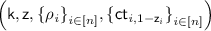

• :

  • Sample and .

  • Compute .

  • For all and , compute

    

  • Compute .

  • Output

    

    (4)

    The random coin used in is .

• :

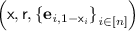  • Parse and as the Eqs. 3 and 4, respectively.

  • For all , set

    

  • Output .

By setting $\ell =\mathsf {poly}(\log \lambda )$, $\mathtt {NCE}$ is correct. Formally, we have the following theorem.

Theorem 2

Let $\ell =\mathsf {poly}(\log \lambda )$. If $\mathtt {CE}$ is correct under obliviously sampled keys, then $\mathtt {NCE}$ is correct.

Proof

Due to the correctness under obliviously sampled keys of $\mathtt {CE}$, the recovery of fails only when happens and coincides with . Thus, the probability of decryption failure is bounded by

Note that at the last step, we used the union bound. Since , the probability is negligible by setting . Therefore $\mathtt {NCE}$ is correct.

Intuition for the Simulators and Security Proof. The description of the simulators of $\mathtt {NCE}$ is somewhat complex. Thus, we give an overview of the security proof for $\mathtt {NCE}$ before describing them. We think this will help readers understand the construction of simulators.

In the proof, we start from the real experiment , where $\mathcal {A}$ is an PPT adversary attacking the security of $\mathtt {NCE}$. We then change the experiment step by step so that, in the final experiment, we can generate the ciphertext given to $\mathcal {A}$ without the message m chosen by $\mathcal {A}$, which can later be opened to any message. The simulators are defined so that they simulate the final experiment.

In is of the form

Informally, encapsulates , and is a one-time encryption of $m\in \{0,1\}^\mu$ by . If we can eliminate the information of from the encapsulation part, becomes statistically independent of m. Thus, if we can do that, the security proof is almost complete since in that case, can be simulated without m and later be opened to any message. While we cannot eliminate the entire information of from the encapsulation part, we can eliminate the information of $\mu$ out of n bits of from the encapsulation part, and it is enough to make statistically independent of m. Below, we briefly explain how to do it.

We first change contained in so that every $\mathsf {ct}_{i,b}$ is generated as , and set , where is a random string generated in . We can make this change by the oblivious samplability of $\mathtt {CE}$.

Next, by using the security of $\mathtt {CE}$, we try to change the experiment so that for every $i\in [n]$, and contained in are symmetrically generated in order to eliminate the information of from the encapsulation part. Concretely, for every $i\in [n]$, we try to change from a random string to

Unfortunately, we cannot change the distribution of every because some of is given to $\mathcal {A}$ as a part of . Concretely, for $i\in [n]$ such that , is given to $\mathcal {A}$ and we cannot change the distribution of . On the other hand, for $i\in [n]$ such that , we can change the distribution of .

In order to make clear which index $i\in [n]$ we can change the distribution of , in the proof, we replace with . Then, we can say that for $i\in [n]$ such that , we can change the distribution of . Since is chosen uniformly at random, due to the Chernoff bound, we can ensure that the number of such indices is greater than $\mu$ with overwhelming probability by setting n and $\mu$ appropriately. Namely, we can eliminate the information of $\mu$ out of n bits of from . At this point, becomes statistically independent of m, and we almost complete the security proof. Note that $\mathsf {y}$ itself does not have any information of . To make this fact clear, in the proof, we add another step using the trapdoor collision property of $\mathtt {CE}$ after using the security of $\mathtt {CE}$.

To complete the proof formally, we have to ensure that can later be opened to any message efficiently (i.e., in polynomial time). This is possible by using a matrix ${R}\in \{0,1\}^{\mu \times {n}}$, such that randomly picked $\mu$ out of ${n}$ column vectors of length $\mu$ are linearly independent. For more details, see the formal security proof in Sect. 5.2.

We now show the simulators .

• $\mathsf {Sim}_{\mathsf{1}}\,(1^{\lambda })$:

  • Sample .

  • For all and , sample and compute .

  • Sample ³, and .

  • Compute and sample .

  • For all and , compute

    

  • Output

    

    and .

• $\mathsf {Sim}_{\mathsf{2}}\,(m, st )$:

  • Sample at random from $\{0,1\}^n$ under the condition that and hold for every $i\in [n]$ such that .

  • Compute and .

  • Output

5.2 Security Proof

In this section, we prove the security of $\mathtt {NCE}$. Formally, we prove the following theorem.

Theorem 3

Let and ${n}=8\mu$. If $\mathtt {CE}$ is an obliviously samplable CE, then $\mathtt {NCE}$ is secure.

Proof

Let $\mathcal {A}$ is a PPT adversary attacking the security of $\mathtt {NCE}$. We define a sequence of experiments . Below, for two experiments and , we write (resp. ) to denote that the probability that $\mathcal {A}$ outputs 1 in is negligibly close to (resp. the same as) that in .

• : This experiment is exactly the same as . The detailed description is as follows. 1. The experiment first samples and . Then, for all , it samples . Next, for all and , it computes

  

  It sets

  

  Finally, it runs . Note that is used in the next step.

  2. The experiment samples and . It then computes . For all and , it also computes

  

  It sets

  

  Finally, it outputs .

• : This experiment is the same as except the followings. First, is generated together with a trapdoor of the chameleon hash function $\mathsf {t}$ as instead of . Moreover, all ciphertexts of chameleon encryption are computed by , instead of . Specifically, for every and , the experiment samples and compute . Also, it sets .

Lemma 5

Assuming the oblivious samplability of $\mathtt {CE}$, holds.

Proof

Using $\mathcal {A}$, we construct a reduction algorithm ${\mathcal {A}^{\prime }}^{{O}^*(\cdot ,\cdot )}$ that attacks the oblivious samplability of $\mathtt {CE}$ and makes ${n}$ oracle queries.

• 1. On receiving a hash key , $\mathcal {A}^{\prime }$ generates for every $i\in [n]$ and sets the public key as , where

  

  ${\mathcal {A}^{\prime }}^{{O}^*(\cdot ,\cdot )}$ also sets . Then, ${\mathcal {A}^{\prime }}^{{O}^*(\cdot ,\cdot )}$ runs and obtains m.

• 2. ${\mathcal {A}^{\prime }}^{{O}^*(\cdot ,\cdot )}$ simulates the step 2. of and , and outputs what $\mathcal {A}$ does. Note that the step 2. of is exactly the same as that of .

When playing and , $\mathcal {A}^{\prime }$ perfectly simulates and for $\mathcal {A}$, respectively. By the oblivious samplability of $\mathtt {CE}$,

holds. This proves .

• : This experiment is the same as , except that we replace contained in by .

Because distributes uniformly at random, so does . Therefore, the distribution of the inputs to $\mathcal {A}$ does not change between and , and thus holds.

• : The essential difference from in this experiment is that when is computed by instead of uniformly sampled from $\{0,1\}^\ell$.

  Additionally, each is replaced to from , though this does not change the distribution due to the correctness of $\mathtt {CE}$. After all, for every and , the experiment computes

  

Lemma 6

If $\mathtt {CE}$ is correct and secure, holds.

Proof

This proof is done by hybrid arguments. We define for every $j\in \{0,\ldots ,n\}$ that are intermediate experiments between and as follows.

• : This experiment is exactly the same as except how is generated for every $i\in [n]$. For is generated as in . For is generated as in .

is equal to , and is equal to . In the following, we show for all $j\in [n]$.

In the case of , except negligible probability, distributes identically in and because holds with overwhelming probability due to the correctness of $\mathtt {CE}$. Moreover, is generated in the same way in both experiments. Thus holds.

In the case of , we show by constructing a reduction algorithm $\mathcal {A}^{\prime }$ that uses $\mathcal {A}$ and attacks the security of $\mathtt {CE}$. The description of $\mathcal {A}^{\prime }$ is as follows.

• 1. $\mathcal {A}^{\prime }$ samples and , outputs , and receives . Then, $\mathcal {A}^{\prime }$ generates as follows. $\mathcal {A}^{\prime }$ first samples and sets . For every $(i,b)\in [n]\times \{0,1\}$ such that , $\mathcal {A}^{\prime }$ samples and computes 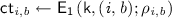. $\mathcal {A}^{\prime }$ sets ,

  

  Finally, $\mathcal {A}^{\prime }$ runs . Note that since we consider the case of , and thus $\mathcal {A}^{\prime }$ generates by itself for every $i\in [n]$.

• 2. $\mathcal {A}^{\prime }$ computes . For , $\mathcal {A}^{\prime }$ computes as in , and for , it does as in . For , $\mathcal {A}^{\prime }$ computes and sets . Finally, $\mathcal {A}^{\prime }$ sets

  

  and outputs .

When playing , $\mathcal {A}^{\prime }$ simulates for $\mathcal {A}$. Also, when playing , $\mathcal {A}^{\prime }$ simulates for $\mathcal {A}$. By the security of $\mathtt {CE}$,

holds. From the above, we have

We can conclude .

• : This experiment is the same as except how $\mathsf {y}$ and are computed. In this experiment, $\mathsf {y}$ is computed as . Moreover, the randomness contained in is replaced with .

Due to the trapdoor collision property of $\mathtt {CE}$, the view of $\mathcal {A}$ does not change between and . Thus, holds.

• : This experiment is the same as , except that is replaced with . Moreover, the experiment computes as , and replaces in with , where is a uniformly random string sampled from $\{0,1\}^n$ under the following two conditions:

  – holds.

  – holds for every $i\in [n]$ such that .

Before showing , we review a basic lemma on inversion sampling.

Lemma 7

For a function $f:\mathcal {X}\rightarrow \mathcal {Y}$, we define two distributions $\mathcal {D}_1$ and $\mathcal {D}_2$ as and , where $f^{-1}(y)$ denotes the set of pre-images of y. Then, $\mathcal {D}_1$ and $\mathcal {D}_2$ are identical.

Furthermore, we define a distribution $\mathcal {D}_3$ as . If f has a property that f(x) distributes uniformly at random over $\mathcal {Y}$ if the input x distributes uniformly at random over $\mathcal {X}$, $\mathcal {D}_1$ and $\mathcal {D}_3$ are identical.

Lemma 8

holds.

Proof

According to the Chernoff bound on ,

holds for any $\delta >0$. By taking $\delta =1-\frac{2\mu }{{n}}$, we have

Below, we show that in has the same distribution as in in the case of , and complete the proof of this lemma.

We first introduce some notations. For an integer ordered set $\mathcal {I}\subset [n]$, we define $R_{\mathcal {I}}$ as the restriction of R to $\mathcal {I}$, that is $R_{\mathcal {I}}=(\mathbf {r}_1|\cdots |\mathbf {r}_{\left|\mathcal {I}\right|})$, where $R=(\mathbf {r}_1|\cdots |\mathbf {r}_n)$. We define in a similar way.

Fix any which satisfies and set . Because $\left|\mathcal {I}\right|\ge \mu$, ${R}_{\mathcal {I}}$ is full rank due to the choice of ${R}$. Hence, ${R}_{\mathcal {I}}\cdot u$ is uniformly random over $\{0,1\}^\mu$ if u is uniformly random over $\{0,1\}^{\left|\mathcal {I}\right|}$.

Then, from Lemma 7 when setting , and , the distribution of and $(u,{w})$ are the same, where , and . Moreover, we have . Since sampled in is a bit string generated by replacing $i_k$-th bit of with k-th bit of u for every $k\in [\left|\mathcal {I}\right|]$, we see that has the same distribution as . also has the same distribution as because ${w}$ is sampled uniformly at random, and thus has the same distribution as . This completes the proof of Lemma 8.

Note that we can sample the above u in polynomial time, by computing a particular solution $v\in \{0,1\}^{\left|\mathcal {I}\right|}$ of ${R}_{\mathcal {I}}\cdot v ={w}$, and add a vector sampled uniformly at random from the kernel of ${R}_{\mathcal {I}}$.

• : This experiment is the same as except that ${w}$ is replaced with . By this change, is of the form

  

  Moreover, contained in is sampled so that holds.

Since ${w}$ is uniformly at random, so is . Thus, holds.

We see that is the same as . Put all the above arguments together, we have

Hence $\mathtt {NCE}$ is secure. This completes the proof of Theorem 3.

5.3 Ciphertext Rate

Finally, we evaluate the ciphertext rate of $\mathtt {NCE}$. From Theorem 2, in order to make $\mathtt {NCE}$ correct, it is sufficient to set . Moreover, from Theorem 3, in order to make $\mathtt {NCE}$ secure, it is sufficient to set and ${n}=8\mu$. In this setting, the ciphertext length of $\mathtt {NCE}$ is . Note that we assume a group element of $\mathbb {G}$ is described as a -bit string. Then, the ciphertext rate of $\mathtt {NCE}$ is evaluated as

6 Full Construction of Proposed NCE

In the basic construction, we construct an NCE scheme with correctness , by setting which is the output length of (and thus ) of the underlying $\mathtt {CE}$. Of course, if we set $\ell$ to , we can make the ciphertext rate of the resulting NCE scheme . However, this modification also affects the correctness of the resulting NCE scheme. $\gamma$ is no longer , and is at most .

Fortunately, we can amplify the correctness of the scheme to from enough large constant without changing the ciphertext rate. For that purpose, we use a constant-rate error-correcting code which can correct errors up to some constant fraction. Concretely, we modify the scheme as follows. In the encryption, we first encode the plaintext by the error-correcting code and parse it into blocks of length $\mu$. Then, we encrypt each block by the $\gamma$-correct NCE scheme for a constant $\gamma$ using different public keys. The decryption is done naturally, i.e., decrypt each ciphertext, concatenate them, and decode it. The ciphertext rate is still because the rate of error-correcting code is constant.

This block-wise encryption technique not only amplifies the correctness but also reduces the public key size. In the basic construction, the size of a public key depends on the length of a message quadratically. However, by applying the block-wise encryption technique, it becomes linear in the length of a message.

The description of the full construction is as follows. Let be a constant-rate error-correcting code which can correct errors up to $\epsilon$-fraction of the codeword where $\epsilon >0$ is some constant.

Specifically, given a message , outputs a codeword . If , . The rate of $\mathtt {ECC}$ is some constant N/M.

Let be an NCE scheme whose message space is $\{0,1\}^{\mu }$, ciphertext rate is , and correctness is $\gamma =1-\frac{\epsilon }{2}$. We construct as follows. The message space of $\overrightarrow{\mathtt {NCE}}$ is $\{0,1\}^{\mu M}$.

• :

  • Parse the given random coin to .

  • For all , generate key pairs .

  • Output and .

• :

  • Parse .

  • Compute and parse .

  • For all , compute .

  • Output .

• : 

  • For all , Compute .

  • Concatenate them as .

  • Output .

• :

  • For all , compute ,

  • Output , , and .

• :

  • Compute and parse .

  • For all , compute .

  • Output and .

Correctness. We can prove the correctness of $\overrightarrow{\mathtt {NCE}}$ by the Chernoff bound. Formally, we have the following theorem. See the full version for the proof.

Theorem 4

Let $\mathtt {ECC}$ be an constant-rate error-correcting code which can correct errors up to $\epsilon$-fraction of a codeword. Let $\mathtt {NCE}$ be a $\gamma$-correct NCE scheme, where $\gamma =1-\frac{\epsilon }{2}$. If the number of parsed codeword , the above $\overrightarrow{\mathtt {NCE}}$ is correct.

Security. For the security of , we have the following theorem. Since we can prove it via a straightforward hybrid argument, we omit it.

Theorem 5

If $\mathtt {NCE}$ is an secure NCE scheme, then $\overrightarrow{\mathtt {NCE}}$ is also secure.

Ciphertext Rate. Since rate of the error-correcting code is constant, the ciphertext rate of $\overrightarrow{\mathtt {NCE}}$ is .